Non-linear diffusion with stochastic resetting

Abstract

Resetting or restart, when applied to a stochastic process, usually brings its dynamics to a time-independent stationary state. In turn, the optimal resetting rate makes the mean time to reach a target to be the shortest one. These and other intriguing problems have been intensively studied in the case of ordinary diffusive processes over the last decade. In this paper we consider the influence of stochastic resetting on a diffusive motion modeled in terms of the non-linear differential equation. The reason for its non-linearity is the power-law dependence of the diffusion coefficient on the probability density function or, in another context, the concentration of particles. We briefly outline this issue at first to prepare the foundations for our further considerations. Then, we derive an exact formula for the mean squared displacement and demonstrate how it attains the steady-state value under the influence of exponential resetting. This mechanism brings also about that the spatial support of the probability density function, which for the free non-linear diffusion is confined to the set of a finite measure, tends to span the entire domain of real numbers. In addition, we explore the first-passage properties for the non-linear diffusion intermittent by the exponential resetting and find analytical expressions for the mean first-passage time and determine numerically the optimal resetting rate which minimizes the mean time needed for a particle to reach a pre-determined target. Finally, we test and confirm the universal property that the relative fluctuation in the mean first-passage time of optimally restarted non-linear diffusion is equal to unity.

Keywords non-linear diffusion  $\cdot$ mean squared displacement  $\cdot$ probability density  $\cdot$ stochastic resetting  $\cdot$ mean first-passage time

1 Introduction

Over the past few years a concept of stochastic resetting turned into a paradigm in such diverse disciplines as statistical physics [1] and stochastic thermodynamics [2, 3, 4], biological physics [5, 6], biochemistry [7, 8], biology [9] and computer science [10, 11, 12, 13] drawing a significant attention among scientific community. Resetting/restart is the procedure that stops and returns a considered process at random instants of time to some pre-determined state, from which it starts over again. Comprehensive studies performed in the last decade have confirmed that this mechanism generates nontrivial effects on dynamical systems [14]. For instance, a system of which we certainly know that relaxes to the equilibrium state, when subject to stochastic resetting, generically attains the time-independent stationary state. Another property of resetting is to make a first-passage process finite in time which might be difficult in some other circumstances.

A special type of processes for which the steady-state and the first-passage properties have been intensively explored in the presence of resetting is diffusion. Intensified research on this topic began with a publication of a seminal work on the canonical model of diffusion through the agency of the exponential resetting [15] (see also [16]). Since its original formulation this model has been gradually extended to include other essential features of the diffusive motion as well as the alternative variants of stochastic resetting. Foremost examples comprise the models that consider diffusion confined in bounded domains [17, 18] and in external potentials with a constant [19, 20, 21] and a space-dependent diffusivity [21], diffusion in arbitrary spacial dimensions [22], under partial absorption [23], and in the presence of interactions [24, 25]. Another category of processes studied for stochastic resetting include anomalous diffusion [26, 27], Lévy flights [28, 29], underdamped, scaled and fractional Brownian motions [30, 31, 32, 33], random walk [34, 35, 36, 37, 38], continuous-time random walk with and without drift [39, 40, 41], telegraphic processes [42] and many others [43, 44, 45].

In the meantime, a few non-exponential resets and apart from them also more realistic mechanisms of stochastic resetting have been proposed. In the former case, where the resetting protocol is assumed to be instantaneous, one considered the diffusive systems with deterministic [46], non-static [47], scale-free [48], intermittent [49], and non-Markovian [50] restarts as well as those with the space and time-dependent resetting rates [51] and in the presence of the power-law resetting time distributions [52]. However, bringing a material particle from one place to another always takes some period of time in real situations. To make the resetting processes more physical and practical form the experimental point of view [53, 54] one has needed to invent completely new solutions in comparison with those discussed so far. Such theoretical ideas that have recently appeared involve returns with a constant or space-dependent velocity [55, 56, 57, 58, 59, 60], a constant or space-dependent acceleration [59, 60], resets with finite time [61] and under the influence of external traps such as confining potentials [62, 63].

Besides studies on the stationary states of diffusive systems affected by resetting events also their first passage properties has been extensively investigated at the same time [64, 65, 66]. This issue is particularly important for the optimal search strategies [67, 68, 69, 70, 71] based on conceptually advanced algorithms dedicated to solve hard combinatorial problems [72]. A typical quantitative measure of efficiency of a search process is the mean-first passage time or, in other words, the time at which a searcher hits a target at an unknown location for the first time on average [73]. The main conclusion arising from the studies conducted in this field is that restart renders the mean first-passage time finite and minimal for the optimal resetting rate [14]. It has been appeared that the most effective search strategy is achieved for the deterministic resetting when the time intervals between resets are of a constant value [51, 65, 66]. Aside from the optimal rate of resetting there exists a certain value of the exponent present in the power-law distribution of waiting times between resets which for an ordinarily diffusing particle minimizes its mean first-passage time from an initial to a given target position [52]. The first-passage time problem under stochastic resetting has also been analyzed in a presence of various external potentials [74, 21, 75], in bounded domains [76, 77] and under restart with branching [78].

In all the aspects considered above the diffusive motion intermittent by stochastic resetting was governed by the linear partial differential equations. As we know so far, the only exception to this rule is the non-linear dynamical system such as chaotic Lorenz model analyzed in the reference [79]. However, this dynamics have nothing to do with a diffusive motion. Thus, in the present paper we investigate the effect of exponential resetting on both the steady-state and the first-passage properties of the non-linear diffusion. Here, our intention is to consider the most fundamental aspects of this problem and indicate those we intend to explore in the future.

In this paper we focus on a special variant of the non-linear diffusion equation in which a diffusion coefficient depends on the probability density or concentration of particles through the power-law relation with a constant exponent. We show that the mean squared displacement and the probability density function resulting from the solution of the non-linear differential equation have their counterparts in the form of appropriate steady-state expressions as long as the non-linear diffusion proceeds under the influence of exponential resetting. By contrast with the ordinary diffusion a domain of the probability density function for the non-linear diffusion is restricted to a finite support, outside of which this function disappears. However, the mechanism of exponential resetting makes the support of the stationary probability density function extended to the entire domain of real numbers. We will display this effect on the example of the exact as well as approximate solutions of the non-linear diffusion equation. They have been obtained for peculiar values of the power-law exponent that characterizes the dependence of the diffusion coefficient on the probability density. In the second part of the paper we analyse the mean hitting time problem and find the exact and approximate formulae for the mean first-passage time to the target localized at the origin of the semi-infinite interval. Moreover, we also determine the optimal resetting rate that minimizes this time and its dependence on the power-low exponent and the distance from an initial position to the target. In addition, the relative standard deviation associated with the mean first-passage time of the optimally restarted non-linear diffusion at the constant rate is shown to be equal to unity.

The paper is organized as follows. In the next section we give a brief overview of the non-linear diffusion equation with a power-law dependence of the diffusion coefficient on the concentration/probability density. The informative content of this section is enough to be used in subsequent parts of the paper. Sec. 3 is reserved to examine the basic stationary properties of the non-linear diffusion under the exponential resetting from a viewpoint of the mean squared displacement and the probability density function. In Sec. 4 we consider the first-passage time properties of the non-linear diffusion interrupted by the exponential resets. We summarize our results in Sec. 5.

2 Non-linear diffusion equation

In what follows we restrict our studies of the non-linear diffusion and its time course under the influence of stochastic resetting to one dimension. Before we formulate a special type of the equation describing this process let us firstly consider its more general form, namely [80]

$$\frac{\partial}{\partial t}p(x,t)=\frac{\partial}{\partial x}\left(\mathcal{D}\left[\,p(x,t)\right]\frac{\partial}{\partial x}p(x,t)\right).$$ (1)

By definition, this is a non-linear partial differential equation for a function $p(x,t)$, which in a physical sense may stand for, depending on the context, the concentration of diffusing particles, where $x$ is the distance from some initial position and $t$ is the time, or the probability density function (PDF) of finding a diffusing particle in the location $x$ at time $t$. In this paper we will consequently use the latter interpretation. The reason for the non-linear nature of Eq. (1) is a direct dependence of the diffusivity $\mathcal{D}[p(x,t)]$ on the PDF through which it also depends on the variables $x$ and $t$. Therefore, to specify the particular form of Eq. (1) we have yet to establish a specific relationship between the diffusion coefficient and the PDF. Due to many interesting and practical applications that have attracted considerable attention within a scientific community [81] we define this relation by the power-law function

$$\mathcal{D}=\mathcal{D}_{0}\left(\frac{p(x,t)}{p_{0}}\right)^{\sigma}.$$ (2)

In this expression $p_{0}$ denotes a constant reference value of a probability density, whereas $\mathcal{D}_{0}$ is the diffusivity at that reference value. The power-law exponent $\sigma$ is a certain parameter. Only in the particular case for $\sigma\!=\!0$, Eq. (1) converts into a linear diffusion equation with a diffusion constant $\mathcal{D}_{0}$. In turn, if $\sigma\!>\!0$ then Eq. (1) together with Eq. (2) contribute to the non-linear diffusion equation of the special type called the porous medium equation [82]. This differential equation has found many applications in a study of such disparate transport phenomena as compressible gas flow through porous media [83], heat propagation occurring in plasma [84], groundwater flow in fluid mechanics [85], population migration in biological environment [86, 87], the diffusion of grains in granular matter [88] and gravity-driven fluid flow in layered porous media [89], to name but a few examples.

To give Eq. (1) a more convenient form we now rewrite the diffusion coefficient in Eq. (2) so that $\mathcal{D}=Dp^{\sigma}(x,t)$. Here the parameter $D=\mathcal{D}_{0}/p^{\sigma}_{0}$ is the generalized diffusion coefficient of the physical dimension $[D]=\mathrm{L}^{\sigma+2}/\mathrm{T}$, where $\mathrm{L}$ and $\mathrm{T}$ are units of a length and a time, respectively. In consequence, the non-linear diffusion equation is as follows:

$$\frac{\partial}{\partial t}p(t,x)=D\frac{\partial}{\partial x}\left(p^{\sigma}(x,t)\frac{\partial}{\partial x}p(x,t)\right).$$ (3)

A commonly known procedure for solving this class of equations is offered by the method of similarity solutions that utilizes an algebraic symmetry of a differential equation. In order to find its solution we insert into Eq. (3) a similarity transformation of the algebraic form

$$p(x,t\!\mid\!x_{0})=\frac{1}{T(t)}F\left(\frac{x-x_{0}}{T(t)}\right)\equiv\frac{F(z)}{T(t)},\;\;\text{with}\;\;z=\frac{x-x_{0}}{T(t)}$$ (4)

for the PDF of appearing a particle in $x$ at time $t$, if it was localized in the initial position $x_{0}$ at time $t\!=\!0$. In this way we effectively reduce the original partial differential equation for the non-linear diffusion to the system of two ordinary differential equations for the separate functions $T(t)$ and $F(z)$ which are relatively easy to solve. We omit detailed calculations here and refer the interested reader to [80], where the discussed method is accessibly explained. Thus, as the final result we obtain

$$p(x,t\!\mid\!x_{0}) =\frac{1}{T(t)}\left[a-\frac{b\sigma}{2D}\left(\frac{x-x_{0}}{T(t)}\right)^{2}\right]^{\frac{1}{\sigma}},\;\;\text{with}$$ (5)

$$T(t) =[b(\sigma+2)t]^{\frac{1}{\sigma+2}},$$

where $a$ and $b$ are arbitrary integration constants. Their specific values can be determined by adopting suitable boundary conditions. For example, if we set $a\!=\!1$, with no substantiation for now, and impose the normalization condition $\int_{-\infty}^{\infty}p(x,t\!\mid\!x_{0})dx=1$ on Eq.5, performing appropriate integration with a help of the Euler beta function $\mathrm{B}(\nu,\mu)=\frac{\Gamma(\nu)\Gamma(\mu)}{\Gamma(\nu+\mu)}=2\int_{0}^{1}z^{2\nu-1}(1-z^{2})^{\mu-1}dz$ [90], we find the unknown $b$ and eventually a typical solution of Eq.(3) in the Zel’dovitch-Barenblatt-Pattle algebraic form [91, 92, 93]

$$p(x,t\!\mid\!x_{0})=\frac{\mathcal{A}(\sigma)}{(Dt)^{\frac{1}{\sigma+2}}}\left[1-\mathcal{B}(\sigma)\frac{(x-x_{0})^{2}}{(Dt)^{\frac{2}{\sigma+2}}}\right]^{\frac{1}{\sigma}},$$ (6)

where the two $\sigma$-dependent coefficients in the above PDF are

$$\mathcal{A}(\sigma)=\left[\sqrt{\frac{\sigma}{2\pi(\sigma+2)}}\,\frac{\Gamma\left(\frac{1}{\sigma}+\frac{3}{2}\right)}{\Gamma\left(\frac{1}{\sigma}+1\right)}\right]^{\frac{2}{\sigma+2}}$$ (7)

and

$$\mathcal{B}(\sigma)=\sigma\left[\frac{1}{2(\sigma+2)}\right]^{\frac{2}{\sigma+2}}\left[\frac{\sqrt{\pi}\,\Gamma\left(\frac{1}{\sigma}+1\right)}{\sqrt{\sigma}\,\Gamma\left(\frac{1}{\sigma}+\frac{3}{2}\right)}\right]^{\frac{2\sigma}{\sigma+2}}.$$ (8)

The plot in Fig. 1 displaces profiles of the PDF in two different moments of time. A supplementary comment is necessary at this point. The formulae given in Eqs. (5) and (6) do not guarantee that the PDF for the non-linear diffusion is always a real and positive function of $x$ as it should be by virtue of a very definition of the probability density $p(x,t\!\mid\!x_{0})\geqslant 0$. For this reason we need to assume the additional requirement that the PDF can only be determined on the finite support $\mid\!x-x_{0}\!\mid\leqslant\mathcal{B}^{-\frac{1}{2}}(Dt)^{\frac{1}{\sigma+2}}$. Everywhere outside this interval the PDF vanishes and such a property was taken into account when performing integration in the normalization condition to figure out the parameter $b$.

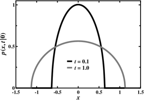
Figure 1: Probability distribution function described by Eq. (6) in two different moments of time. Here we assumed the parameter $\sigma\!=\!2.0$ and the diffusion coefficients $D\!=\!1.0$.

We are still aware choosing a value of the parameter $a\!=\!1$ without any explanation which may raise serious reservation. The argument behind such a choice is as follows. Supposing $\sigma$ goes to zero and using the assertion that $\lim_{z\to\infty}\frac{\Gamma(z+\alpha)}{\Gamma(z+\beta)}z^{\beta-\alpha}=1$ (see [90]) along with $\alpha=3/2$, $\beta=1$ and $z=1/\sigma$, we obtain from Eqs. (7) and (8) that $\mathcal{A}\!=\!1\!/\!\sqrt{4\pi}$ and $\mathcal{B}\!=\!\lim_{\sigma\to 0}\sigma\!/\!4$. Simultaneously, expressing the right-hand site of Eq. (6) through the limit definition of the exponential function $\mathrm{e}^{-z}=\lim_{n\to\infty}(1-\frac{z}{n})^{n}$ for $n\!=\!1/\sigma$, we immediately retrieve the Gaussian distribution

$$p(x,t\!\mid\!x_{0})=\frac{1}{\sqrt{4\pi Dt}}\exp\left[-\frac{(x-x_{0})^{2}}{4Dt}\right].$$ (9)

The above function is a fundamental solution of the linear partial differential equation for a free diffusion given by Eq. (3) whenever $\sigma\!=\!0$ with the initial condition $p(x,0\mid x_{0})\!=\!\delta(x-x_{0})$. This result justifies our decision to set $a\!=\!1$.

One of the crucial quantities characterising a diffusive motion is the mean squared displacement (MSD). It is the most common measure of the deviation of the position $x$ of a diffusing particle with respect to some reference position $x_{0}$ over time. When $x_{0}\!=\!0$ then MSD is defined as $\left<x^{2}(t)\right>\!=\!\int_{-\infty}^{\infty}x^{2}p(x,t)\mathrm{d}x$. For the free linear diffusion in one dimension its MSD is $\left<x^{2}(t)\right>\!=\!2Dt$, whereas in the case of the non-linear diffusion, for which the PDF is given by Eq. (6) we get

$$\left<x^{2}(t)\right>=D_{\sigma}t^{\frac{2}{\sigma+2}},$$ (10)

where the coefficient

$$D_{\sigma}=\frac{[2D(\sigma+2)]^{\frac{2}{\sigma+2}}}{3\sigma+2}\left[\frac{\sqrt{\sigma}\,\Gamma\left(\frac{1}{\sigma}+\frac{3}{2}\right)}{\sqrt{\pi}\,\Gamma\left(\frac{1}{\sigma}+1\right)}\right]^{\frac{2\sigma}{\sigma+2}}.$$ (11)

Again, if $\sigma\!\to\!0$ the above equations converge to the standard MSD for the ordinary diffusion. Let us emphasize that contrary to this type of diffusion, the MSD characterising the time course of the non-linear diffusion scales with the time according to the power-law relation given by Eq. (10). Moreover, if $\sigma\!>\!0$ then the power-law exponent in this equation is less than unity which indicates that the non-linear diffusion belongs to the class of the subdiffusive processes.

In the next part of the paper we explain how the presence of stochastic resetting affects the MSD, Eq. (10), and the PDF, Eq. (6), that quantify the basic properties of each diffusive motion including the non-linear diffusion as a special case.

3 Non-linear diffusion with stochastic resetting

A concept of stochastic resetting emerges from renewal theory being a part of a more extensive theory of probability [94]. Following this theory resetting is a mechanism that interrupts a random process at random instants of time in such a way the process is stopped and restarted anew from a given initial state. Here, we focus on the simplest version of this mechanism assuming that the reset events happen instantaneously. Alternative scenarios of the stochastic resetting regarding the non-linear diffusion will be analysed in successive papers.

Let us firstly consider a particle that executes any diffusive motion between reset events. The renewal theory implicates that the PDF to find the particle at location $x$ at time $t$, if it started from the initial position $x_{0}$ is

$$p_{r}(x,t\!\mid\!x_{0})=\int_{0}^{t}\Phi(t-\tau)p(x,t-\tau\!\mid\!x_{0})R(\tau)\mathrm{d}\tau,$$ (12)

where $p(x,t\!\mid\!x_{0})$ corresponds to the PDF for a free diffusion [49]. We supposed in the above equation without loss of generality that the particle is reset to $x_{0}$ although this location can be arbitrary in a space. The function

$$\Phi(t)=\int_{t}^{\infty}\varphi(\tau)\mathrm{d}\tau=1-\int_{0}^{t}\varphi(\tau)\mathrm{d}\tau,$$ (13)

in Eq. (12) denotes the probability (the survival probability) stating that no resetting event occurs between two moments of time $0$ and $t$ and it is expressed by the time integral of the distribution $\varphi(t)$ of waiting times between resets. This quantity is an essential component of the integral equation

$$\varphi_{n}(t)=\int_{0}^{t}\varphi(t-\tau)\varphi_{n-1}(\tau)\mathrm{d}\tau,$$ (14)

that defines the probability $\varphi_{n}(t)$ that the $n$th reset event happens at time $t$ if the $(n-1$)th event occurred with the probability $\varphi_{n-1}(\tau)$ at the previous moment of time $\tau$. The last quantity in Eq. (12) is the probability

$$R(t)=\delta(t)+k(t),$$ (15)

of resetting events provided that the diffusion process starts with a reset event where the $\delta$-distribution accounts for the initial condition and

$$k(t)=\sum\limits_{n=1}^{\infty}\varphi_{n}(t)$$ (16)

stands for the rate of resetting events. To determine this quantity we have to solve at first the recursive relation in Eq. (14). Due to the presence of the time convolution in this equation we are capable of finding its solution in the Laplace domain. The result is as follows

$$\tilde{\varphi}_{n}(s)=\tilde{\varphi}^{n}(s),$$ (17)

where $\tilde{\varphi}(s)\!\equiv\!\int_{0}^{\infty}\varphi(s)\exp(-st)\mathrm{d}t$ is the Laplace transform for which the convolution theorem has been applied. It states that the Laplace transform of the convolution of two functions results in the product of their Laplace transforms. Therefore, writing Eq. (16) in the Laplace domain along with Eq. (16) and carrying out a summation of the geometric series we obtain the Laplace transform of the rate

$$\tilde{k}(s)=\frac{\tilde{\varphi}(s)}{1-\tilde{\varphi}(s)}.$$ (18)

Now, if we plugin Eq. (15) into the primary Eq. (12) then the PDF with the stochastic resetting takes the following form

$$p_{r}(x,t\!\mid\!x_{0})=\Phi(t)p(x,t\!\mid\!x_{0})+\int_{0}^{t}k(\tau)\Phi(t-\tau)p(x,t-\tau\!\mid\!x_{0})\mathrm{d}\tau.$$ (19)

For the particular case of the exponential (Poissonian) resetting, we focus in the present paper on, the probability distribution of waiting times between resets, namely

$$\varphi(t)=r\mathrm{e}^{-rt},$$ (20)

corresponds to the exponential distribution where $r$ denotes a constant rate at which a diffusive particle is reset to the initial position $x_{0}$. After making calculations of the integral in Eq. (13) we figure out the probability of no resets up to time $t$ is given by $\Phi(t)\!=\!\mathrm{e}^{-rt}$. On the other hand, the Laplace transform of the function in Eq. (20) is $\tilde{\varphi}(s)\!=\!r/(s+r)$ and in consequence the rate of the exponential resetting in the Laplace domain, Eq. (18), takes the following form, i.e. $\tilde{k}(s)\!=\!r/s$. Hence, performing the inverse Laplace transform we arrive at the simple result that $k(t)\!=\!r$, whereas the PDF in Eq. (19) for any diffusion with the Poissonian resetting is now

$$p_{r}(x,t\!\mid\!x_{0})=\mathrm{e}^{-rt}p(x,t\!\mid\!x_{0})+r\int_{0}^{t}\mathrm{e}^{-r\tau}p(x,\tau\!\mid\!x_{0})\mathrm{d}\tau.$$ (21)

The first component on the right-hand site refers to the trajectories of the process without resets having occurred up to time $t$ with the probability $\mathrm{e}^{-rt}$, whereas the second one corresponds to the phase of motion when the last resetting event took place at $t\!-\!\tau$ with the probability $r\mathrm{e}^{-rt}$. The above equation constitutes the starting point for the analysis of the MSD and the PDF for the non-linear diffusion under the influence of the exponential resetting we will conduct in consecutive subsections.

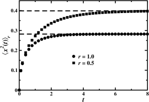
Figure 2: Time course of the MSD $\left<x^{2}(t)\right>_{r}$ for the non-linear diffusion with exponential resetting determined by two various resetting rates $r\!=\!0.5$ and $1.0$. Striving for the MSD to attain stationary values (dashed lines) is an inherent feature of diffusive motions and in general stochastic processes that proceed under the influence of restart protocols.

3.1 Mean squared displacement

Multiplying Eq. (21) by $x^{2}$ and performing integration over the variable $x$, we obtain the equation for the MSD:

$$\left<x^{2}(t)\right>_{r}=\mathrm{e}^{-rt}\left<x^{2}(t)\right>+r\int_{0}^{t}\mathrm{d}\tau\mathrm{e}^{-r\tau}\left<x^{2}(\tau)\right>.$$ (22)

The substitution of Eq. (10) to the above formula leads after elementary calculations to the exact result:

$$\left<x^{2}(t)\right>_{r}=D_{\sigma}t^{\frac{2}{\sigma+2}}\mathrm{e}^{-rt}+D_{\sigma}r^{-\frac{2}{\sigma+2}}\gamma\left(\frac{\sigma+4}{\sigma+2},rt\right),$$ (23)

where $\gamma(\alpha,z)\!=\!\int_{0}^{z}u^{\alpha-1}\mathrm{e}^{-u}\mathrm{d}u$ is the lower incomplete gamma function. Its asymptotic expansion for $z\!\to\!\infty$ is

$$\gamma(\alpha,z)\simeq\Gamma(\alpha)-z^{\alpha-1}\mathrm{e}^{-z}+(1-\alpha)z^{\alpha-2}\mathrm{e}^{-z}$$ (24)

where $\Gamma(\alpha)\!=\!\int_{0}^{\infty}u^{\alpha-1}\mathrm{e}^{-u}\mathrm{d}u$ is the complete gamma function which is represented here by the Euler integral of the second kind. Using this expansion in Eq. (23) we obtain the asymptotic expression for the MSD

$$\left<x^{2}(t)\right>_{r}\simeq D_{\sigma}r^{-\frac{2}{\sigma+2}}\left[\Gamma\left(\frac{\sigma+4}{\sigma+2}\right)-\frac{2}{\sigma+2}(rt)^{-\frac{\sigma}{\sigma+2}}\mathrm{e}^{-rt}\right].$$ (25)

In turn, when $t\!\rightarrow\!\infty$ the MSD rapidly converges to the stationary state:

$$\left<x^{2}(t\!\to\!\infty)\right>_{r}=D_{\sigma}r^{-\frac{2}{\sigma+2}}\Gamma\left(\frac{\sigma+4}{\sigma+2}\right)$$ (26)

In the special case for $\sigma\!\to\!0$ we reconstruct from Eq. (26) the exact result for the ordinary diffusion with the Poissonian resetting where it is known that $\left<x^{2}(t)\right>_{r}\!=\!2D/r$. Fig. 2 displays the time course of the MSD as described by Eq. (23) for two different values of the resetting rates, $r\!=\!0.5$ and $1.0$. We assumed here that the diffusion coefficient $D\!=\!1.0$, while the parameter $\sigma\!=\!2.0$. The dashed lines indicate the stationary values of the MSD and their location is established in accord with Eq. (26).

3.2 Probability density function

From the very beginning we posit that the parameter $\sigma$ in Eq. (2) is assumed to be non-negative. By virtue of this requirement, the two $\sigma$-dependent coefficients in Eq. (6), namely $\mathcal{A}(\sigma)$ and $\mathcal{B}(\sigma)$ (see Eqs. (7) and (8), respectively), are also non-negative and real. In addition, the following condition $Dt\geqslant(\sqrt{\mathcal{B}(\sigma)}\mid\!x-x_{0}\!\mid)^{\sigma+2}$ has to be satisfied to make the PDF in Eq. (6) positive and real as the function depending on time. Moreover, the same condition will turn out to be very crucial concerning integration performed over the time variable in Eq. (21).

To proceed, let us define the above restriction through the Heviside step function $\Theta(z)$ which is equal to 1 if $z\geqslant 0$ and 0 if $z<0$, and rewrite Eq. (6) in the following form:

$$p(x,t\!\mid\!x_{0})=\Theta\!\left(t-D^{-1}(\sqrt{\mathcal{B}(\sigma)}\mid\!x-x_{0}\!\mid)^{\sigma+2}\right)\frac{\mathcal{A}(\sigma)}{(Dt)^{\frac{1}{\sigma+2}}}\left[1-\mathcal{B}(\sigma)\frac{(x-x_{0})^{2}}{(Dt)^{\frac{2}{\sigma+2}}}\right]^{\frac{1}{\sigma}}.$$ (27)

If we now plugin this formula into Eq. (21) and legally neglect its first component supposing that $t\to\infty$, we obtain

$$p_{r}(x\!\mid\!x_{0})=r\int_{\xi(x,\sigma)}^{\infty}\frac{\mathcal{A}(\sigma)}{(Dt)^{\frac{1}{\sigma+2}}}\left[1-\left(\frac{\xi(x,\sigma)}{t}\right)^{\frac{2}{\sigma+2}}\right]^{\frac{1}{\sigma}}\exp(-rt)\,\mathrm{d}t,$$ (28)

where the auxiliary function $\xi(x,\sigma)\!=\!D^{-1}(\sqrt{\mathcal{B}(\sigma)}\mid\!x-x_{0}\!\mid)^{\sigma+2}$ allows us to simplify the formal notation. This expression constitutes the starting point for our studies on the steady-state properties of the non-linear diffusion interrupted by the exponential resetting. We explore this problem in the present section whereas the issues related to the first-passage phenomena will be considered in the subsequent section. Note, however, an explicit calculation of the integral appearing in Eq. (28) is no doubt a great challenge for arbitrary values of the parameter $\sigma\!>\!0$. To avoid this difficult task we can make a use of computational techniques utilizing either reasonable approximations or appropriate numerical procedures. Nevertheless, there are a few exceptions from such solutions that concern the exact results.

The case of $\sigma\!=\!\frac{1}{N}$, where $N$ represents any natural number, is rather trivial and it will be not considered in the present paper. While the first exception we begin with refers to the extreme situation when $\sigma\to 0$. In this case $\mathcal{A}\!=\!1/\sqrt{4\pi}$, $\xi(x,\sigma\to 0)=\lim_{\sigma\to 0}\frac{\sigma}{4D}(x-x_{0})^{2}$ and hence the PDF in Eq. (28) takes the following form (see also the discussion in Sec. 2):

$$p_{r}(x\!\mid\!x_{0})=r\int_{0}^{\infty}\frac{1}{\sqrt{4\pi Dt}}\exp\left[-\frac{(x-x_{0})^{2}}{4Dt}\right]\exp(-rt)\,\mathrm{d}t.$$ (29)

Using the more general integral $\int_{0}^{\infty}t^{\mu-1}\exp(-\alpha t^{-\gamma}-\beta t^{\gamma})dt\!=\!\frac{2}{\gamma}\left(\frac{\alpha}{\beta}\right)^{\mu/2\gamma}\mathrm{K}_{\mu/\gamma}(2\sqrt{\alpha\beta})$ with $\alpha,\,\beta\!>\!0$ [90], where $K_{\nu}(z)$ is the modified Bessel function of the second kind, which for $\nu\!=\!1/2$ corresponds to the exponential function, $K_{1/2}(z)\!=\!\sqrt{\frac{\pi}{2z}}\mathrm{e}^{-z}$, we immediately retrieve the stationary probability distribution

$$p_{r}(x\!\mid\!x_{0})=\frac{1}{2}\sqrt{\frac{r}{D}}\exp\left(-\sqrt{\frac{r}{D}}\,\lvert x-x_{0}\rvert\right),$$ (30)

for the ordinary diffusion under the influence of exponential resetting [15]. Let us clearly emphasize that when the parameter $\sigma$ goes to $0$ then simultaneously the initially finite $x$-support of the sub-integral function, i.e. the PDF in Eq. (27), tends to span the entire real axis. In consequence, the $x$-domain of the two-sided exponential PDF in Eq. (30) extends from minus to plus infinity. The same tendency will be observed for the $x$-support of the PDFs with $\sigma\!>\!0$ but, as we will show, a sole mechanism responsible for such a behavior is associated with the exponential restart in a very long time limit.

A relatively simple instance when the integration in Eq. (28 can be exactly performed refers to the parameter $\sigma\!=\!1.0$. In this case the coefficient $\mathcal{A}\!=\!\left(\frac{3}{32}\right)^{1/3}$ and the lower limit of integration $\xi(x,1)\!=\!\frac{2\mid x-x_{0}\mid^{3}}{9D}$, thus the final result is

$$p_{r}(x\!\mid\!x_{0})=\left(\frac{3r}{32D}\right)^{\frac{1}{3}}\left[\Gamma\!\left(\frac{2}{3},\frac{2r}{9D}\!\mid\!x-x_{0}\!\mid^{3}\right)+\left(\frac{2r}{9D}\right)^{\frac{2}{3}}(x-x_{0})^{2}\,\mathrm{Ei}\!\left(-\frac{2r}{9D}\mid\!x-x_{0}\!\mid^{3}\right)\right],$$ (31)

where $\Gamma(\alpha,z)\!=\!\int_{z}^{\infty}u^{\alpha-1}\mathrm{e}^{-u}\mathrm{d}u$ corresponds to the upper incomplete gamma function and $\mathrm{Ei}(-z)\!=\!-\int_{z}^{\infty}u^{-1}\mathrm{e}^{-u}\mathrm{d}u$ stands for the exponential integral function. Note that for $x\!=\!x_{0}$ the above PDF approaches the maximal value $p_{r}(x_{0})\!=\!\left(\frac{3r}{32D}\right)^{\frac{1}{3}}\Gamma\!\left(\frac{2}{3}\right)$, because $\Gamma(z,0)\!=\!\Gamma(z)$ and $\lim_{z\to 0}z^{2}\mathrm{Ei}(-az^{3})\!=\!0$ which can be easy verified by virtue of the l’Hospital theorem. The same result follows from a direct integration in Eq. (28) with $\xi(0,1)\!=\!0$.

In contrast to the previous exceptions a slightly more complicated task of getting the exact result from Eq. (28) refers to the value of the parameter $\sigma\!=\!2.0$. Here, we only show the final expression defining the PDF for the non-linear diffusion intermittent by the exponential resetting which is as follows:

$$p_{r}(x\!\mid\!x_{0})=\frac{\pi r\!\mid\!x-x_{0}\!\mid^{3}}{8\sqrt{2}D}\exp\!\left(-\frac{\pi^{2}r(x-x_{0})^{4}}{32D}\right)\left[\mathrm{K}_{\frac{3}{4}}\!\left(\frac{\pi^{2}r(x-x_{0})^{4}}{32D}\right)-\mathrm{K}_{\frac{1}{4}}\!\left(\frac{\pi^{2}r(x-x_{0})^{4}}{32D}\right)\right].$$ (32)

A detailed description of a derivation of this result is postponed into Appendix where we also prove that $p_{r}(x_{0})\!=\!\left(\frac{r}{D}\right)^{1/4}\Gamma\left(\frac{3}{4}\right)\!/\!\sqrt{\pi}$ for $x\!=\!x_{0}$. The plot displayed in Fig. 3 shows the collection of PDFs for the peculiar values of the parameter $\sigma$ we have considered until now. The points represented by circles, squares and triangles are outcomes obtained from the numerical integration performed in Eq. (28) and the solid lines corresponds to the exact formulae given, respectively, by Eqs. (30), (31) and (32). As expected, there is nothing special about the excellent consistency of the numerical data with the analytical results. Nonetheless our intention at this point was to demonstrate the correctness of the numerical method we will consequently use in this paper.

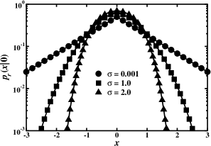
Figure 3: The steady-state PDFs as a function of the position for different values of the parameter $\sigma$. The points marked by circles, squares and triangles are outcomes received from numerical integration performed in Eq. (28). The solid lines represent the exact analytical results given by Eqs. (30), (31) and (32). The fixed values of the diffusion coefficient $D\!=\!1.0$, the initial position $x_{0}\!=\!0$ of a diffusing particle and the resetting rate $r\!=\!1.0$ have been assumed.

These three exact formulae for the PDFs are not only exceptional in the whole class of all possible solutions that might be obtained from Eq. (28) for arbitrary values of the parameter $\sigma$. Together with the numerical tool we have at our disposal, they constitute some kind of certainties for testing the approximate results. In the following two such solutions called the algebraic and the exponential approximations are proposed. The both arise from the fact that the PDF in Eq. (28) must be by definition non-negative and real quantity and this requirement is met if and only if $\xi(x,\sigma)\!\leqslant\!t$. Hence, we can use as the first approximation the power-law expansion $(1-z)^{\alpha}\!\simeq\!1-\alpha z$ with $\mid\!z\!\mid<1$ for the algebraic approximation and the alternative relation $(1-z)^{\alpha}\!\simeq\!\exp(-\alpha z)$ for the exponential approximation.

Let us consider at first the algebraic approximation. In this case the PDF given by Eq. (28) takes the following form:

$$p_{r}(x\!\mid\!x_{0})\simeq r\int_{\xi(x,\sigma)}^{\infty}\frac{\mathcal{A}(\sigma)}{(Dt)^{\frac{1}{\sigma+2}}}\left[1-\frac{1}{\sigma}\left(\frac{\xi(x,\sigma)}{t}\right)^{\frac{2}{\sigma+2}}\right]\exp(-rt)\,\mathrm{d}t,$$ (33)

Now, we can proceed much the same as in a derivation of Eq. (31). Decomposing the above integral into two independent parts and calculating each of them separately, we obtain after elementary operations that

$$p_{r}(x\!\mid\!x_{0})\simeq\mathcal{A}(\sigma)\left(\frac{r}{D}\right)^{\frac{1}{\sigma+2}}\left[\Gamma\left(\frac{\sigma+1}{\sigma+2},r\xi(x,\sigma)\right)-\frac{1}{\sigma}(r\xi(x,\sigma))^{\frac{2}{\sigma+2}}\Gamma\left(\frac{\sigma-1}{\sigma+2},r\xi(x,\sigma)\right)\right]$$ (34)

In the last step we can extract the first incomplete gamma function in front of the square bracket recasting the above formula as the power-law equation and eventually insert in it the explicit form of the auxiliary function $\xi(x,\sigma)$. Therefore, the final result is

$$p_{r}(x\!\mid\!x_{0})\simeq\mathcal{A}(\sigma)\left(\frac{r}{D}\right)^{\frac{1}{\sigma+2}}\Gamma\left(\frac{\sigma+1}{\sigma+2},\frac{r}{D}\zeta(x,\sigma)\right)\left[1-\left(\frac{r}{D}\zeta(x,\sigma)\right)^{\frac{2}{\sigma+2}}\frac{\Gamma\left(\frac{\sigma-1}{\sigma+2},\frac{r}{D}\zeta(x,\sigma)\right)}{\Gamma\left(\frac{\sigma+1}{\sigma+2},\frac{r}{D}\zeta(x,\sigma)\right)}\right]^{\frac{1}{\sigma}},$$ (35)

where we have defined the new function $\zeta(x,\sigma)\!=\!(\sqrt{\mathcal{B}(\sigma)}\mid\!x-x_{0}\!\mid)^{\sigma+2}$ for brevity of the notation. It is clear that if $x\!=\!x_{0}$ then $\zeta(x_{0},\sigma)\!=\!0$ and hence the incomplete gamma function $\Gamma(z,0)\!=\!\Gamma(z)$. We infer from these two properties that

$$p_{r}(x_{0})\simeq\mathcal{A}(\sigma)\left(\frac{r}{D}\right)^{\frac{1}{\sigma+2}}\Gamma\left(\frac{\sigma+1}{\sigma+2}\right).$$ (36)

The plot of the PDF given by Eq. (35) for disparate values of the parameter $\sigma$ falling in the range between $1.0$ and $2.0$ is shown in Fig. 4. Here, we present the compatibility of the algebraic approximation of the PDF (solid lines) with data represented by points obtained from the numerical integration conducted in Eq. (28) for the non-linear diffusion with the resetting rate $r\!=\!1.0$. In addition, we have also verified that the graph of the function plotted according to the approximate formula in Eq. (35) deviates from the numerical results whenever the parameter $\sigma\!<\!1.0$. This fact gives rise to a necessity of finding an appropriate expression for the PDF which could be also applicable in the range of the parameter $\sigma$ between $0$ and $1.0$. We will not resolve this problem in the present paper. Apart from this we conclude that the function in Eq. (35 cannot be converted to the canonical form given by Eq. (30) for $\sigma\to 0$.

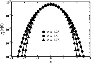
Figure 4: The steady-state PDFs as a function of the position for different values of the parameter $\sigma$ in the range between $1.0$ to $2.0$. The points marked by circles, squares and triangles are outcomes received from the numerical integration performed in Eq. (28). The solid lines represent the approximate analytical result given by Eqs. (35). The fixed values of the diffusion coefficient $D\!=\!1.0$, the initial position $x_{0}\!=\!0$ of a diffusing particle and the resetting rate $r\!=\!1.0$ have been assumed.

Let us now turn to the second case of the exponential approximation according to which the term enclosed within square bracket in Eq. (6) can be replaced by the exponential function

$$p(x,t\!\mid\!x_{0})\simeq\frac{\mathcal{A}(\sigma)}{(Dt)^{\frac{1}{\sigma+2}}}\exp\left[-\frac{\mathcal{B}(\sigma)(x-x_{0})^{2}}{\sigma(Dt)^{\frac{2}{\sigma+2}}}\right].$$ (37)

The substitution of the above formula into Eq. (21) with neglecting of the first component in this equation leads to

$$p_{r}(x,t\!\mid\!x_{0})\simeq r\mathcal{A}(\sigma)\int_{0}^{t}\mathrm{d}\tau\,(D\tau)^{-\frac{1}{\sigma+2}}\exp[-\theta(\tau)],$$ (38)

where we defined the function $\theta(\tau)\!=\!r\tau+\frac{\mathcal{B}(\sigma)(x-x_{0})^{2}}{\sigma(D\tau)^{\frac{2}{\sigma+2}}}$ that poses a single minimum at

$$\tau_{0}=\frac{1}{D^{\frac{2}{\sigma+4}}}\left[\frac{2\mathcal{B}(\sigma)(x-x_{0})^{2}}{r\sigma(\sigma+2)}\right]^{\frac{\sigma+2}{\sigma+4}}.$$ (39)

Because of the condition $0\ll\tau_{0}\ll t$ that holds for very long times (in practice, for $t\!\to\!\infty$), we can apply to Eq. (38) the Laplace saddle-point method [95] which after elementary calculations gives the PDF of the following form:

$$p_{r}(x,t\!\mid\!x_{0}) \simeq r\mathcal{A}(\sigma)(D\tau_{0})^{-\frac{1}{\sigma+2}}\exp[-\theta(\tau_{0})]\int_{-\infty}^{\infty}\mathrm{d}\tau\exp\left[-\frac{1}{2}\theta^{\prime\prime}(\tau_{0})(\tau-\tau_{0})^{2}\right]$$

$$=r\mathcal{A}(\sigma)\sqrt{\frac{2\pi}{\theta^{\prime\prime}(\tau_{0})}}\,(D\tau_{0})^{-\frac{1}{\sigma+2}}\exp[-\theta(\tau_{0})],$$ (40)

provided $\theta^{\prime\prime}(\tau_{0})$ is large enough and where the double prime symbolizes a second derivative of the $\theta(\tau)$ with respect to time $\tau$. Note that both conditions refer to the intermediate asymptotic behavior in $x$. In the last step we complement Eq. (40) by substituting to it the coefficient $\mathcal{A}(\sigma)$ given by Eq. (7) and the function $\theta(\tau)$ together with its second derivative over time at the minimum $\tau_{0}$ (see Eq. (39)). In this way we conclude that the steady-state PDF for non-linear diffusion with the exponential resetting is

$$p_{r}(x\!\mid\!x_{0}) \simeq A(\sigma)\left(\frac{r}{D}\right)^{\frac{2}{\sigma+4}}\lvert x-x_{0}\rvert^{\frac{\sigma}{\sigma+4}}\,\mathrm{e}^{-\phi(x)},\;\;\text{with}$$ (41)

$$\phi(x) =B(\sigma)\left[\frac{r}{D}(x-x_{0})^{\sigma+2}\right]^{\frac{2}{\sigma+4}},$$

where now the actual $\sigma$-dependent coefficients are

$$A(\sigma) =\frac{(2\pi)^{\frac{\sigma}{\sigma+4}}}{\sqrt{\sigma+4}}\left[\frac{\Gamma(\leavevmode\resizebox{5.12149pt}{}{$\frac{1}{\sigma}$}+\leavevmode\resizebox{5.12149pt}{}{$1$})}{\sqrt{\sigma}\,\Gamma(\leavevmode\resizebox{5.12149pt}{}{$\frac{1}{\sigma}$}+\leavevmode\resizebox{5.12149pt}{}{$\frac{3}{2}$})}\right]^{\frac{\sigma-4}{\sigma+4}},\,\,\text{and}$$ (42)

$$B(\sigma) =\frac{1}{2}\left(\frac{\sigma+4}{\sigma+2}\right)\left[\sqrt{\frac{2\pi}{\sigma}}\frac{\Gamma(\leavevmode\resizebox{5.12149pt}{}{$\frac{1}{\sigma}$}+\leavevmode\resizebox{5.12149pt}{}{$1$})}{\Gamma(\leavevmode\resizebox{5.12149pt}{}{$\frac{1}{\sigma}$}+\leavevmode\resizebox{5.12149pt}{}{$\frac{3}{2}$})}\right]^{\frac{2\sigma}{\sigma+4}}.$$ (43)

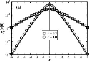
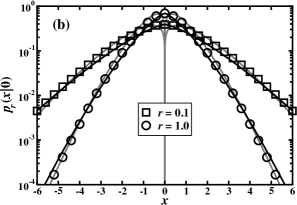
Figure 5: The steady-state PDFs versus the position for two values of the parameter $\sigma\!=\!1.0$ (a) and $2.0$ (b) and two chosen resetting rates $r\!=\!0.1$ (squares) and $1.0$ (circls). Results of numerical integration conducted in Eq. (38) are shown by points. The solid black lines correspond to the PDFs described by Eq. (41) with the pre-exponential factor replaced by the expression obtained in Eq. (44), whereas the gray lines represent the PDF given by Eq. (44). The fixed values of the diffusion coefficient $D\!=\!1.0$ and the initial position $x_{0}\!=\!0$ of a diffusing particle have been assumed.

As $\sigma\rightarrow 0$ these two coefficients take the constant values, respectively, $A(0)\!=\!\frac{1}{2}$ and $B(0)\!=\!1$. In a consequence we observe that unlike the formula given by Eq. (35) the stationary PDF in Eq. (41) bowls down to the canonical two-sided exponential probability distribution shown in Eq. (30).

We underline once again that Eq. (41) corresponds to the intermediate properties of the PDF in $x$, so it ignores the case when $x\!=\!x_{0}$. In order to determine the actual value of $p_{r}(x\!\mid\!x_{0})$ for $x\!=\!x_{0}$ we have to perform the integral in Eq. (38) with $\theta(\tau)\!=\!r\tau$ and $t\!\to\!\infty$. The result is

$$p_{r}(x_{0})=\mathcal{A}(\sigma)\left(\frac{r}{D}\right)^{\frac{1}{\sigma+2}}\Gamma\left(\frac{\sigma+1}{\sigma+2}\right).$$ (44)

Figure 5 exemplifies the steady-state PDFs for the non-linear diffusion with the Poissonian resetting. Here, we supposed two different values of the parameter $\sigma\!=\!1.0$ and $2.0$ and two chosen resetting rates $r\!=\!0.1$ and $1.0$ in the both cases. Due to these plots we show that the data (points) obtained from the numerical integration performed on the basis of Eqs. (37) and (38) are in good agreement with the analytical results (solid black lines) defined by Eq. (41) in which the pre-exponential component was replaced by the expression in Eq. (44). The additional gray lines represent the steady-state PDFs given by a whole function in Eq. (41).

4 Mean hitting time for non-linear diffusion with stochastic resetting

4.1 General method

From now on we turn to the problem of finding the mean time needed for a diffusing particle to reach a target localized at the origin $x\!=\!0$ of the semi-infinite interval if it starts at a position $x\!=\!x_{0}$. The target is thought of as an immobile absorbing point so that when the diffusing particle hits the origin for the first time it remains there forever. In this sense our task is formally equivalent to the first-passage time problem or more precisely the mean time to absorption (MTA). However, we additionally assume that during a diffusive motion the particle is also reset to the initial position $x_{0}$ at a constant rate $r$ with the probability $r\mathrm{e}^{-rt}$. The key quantity associated with the MTA is the survival probability. As for the PDF in Eq. (21) it is also possible to relate the survival probability with the exponential resetting, $Q_{r}$, to that without resetting, $Q$. The resulting equation reads

$$Q_{r}(t\!\mid\!x_{0})=\mathrm{e}^{-rt}Q(t\!\mid\!x_{0})+r\int_{0}^{t}\mathrm{d}\tau\mathrm{e}^{-rt}Q(\tau\!\mid\!x_{0})Q_{r}(t-\tau\!\mid\!x_{0}),$$ (45)

where the first term on the right-hand site corresponds to trajectories without resets whereas the second one represents trajectories in which resetting has occurred [14]. Note that the integral is performed with respect to the time $\tau$ that elapsed since the last reset and there is a convolution of two survival probabilities. The first one refers to the diffusive motion starting from the location $x_{0}$ in the absence of resetting for duration $\tau$ and the second one concerns its continuation starting from the same position with resetting up to time $t\!-\!\tau$. Using the Laplace transformation for the survival probability $\tilde{Q}_{r}(s\!\mid\!x_{0})\!=\!\int_{0}^{\infty}Q_{r}(t\!\mid\!x_{0})\mathrm{e}^{-st}\mathrm{d}t$, we can convert Eq. (45) to the appropriate equation in the Laplace domain:

$$\tilde{Q}_{r}(s\!\mid\!x_{0})=\frac{\tilde{Q}(s+r\!\mid\!x_{0})}{1-r\,\tilde{Q}(s+r\!\mid\!x_{0})}.$$ (46)

The algebraic form of the above equation is especially convenient to determine the MTA for any diffusion process with the Poissonian resetting. Indeed, due to the relation between MTA and the survival probability is defined in the following form, $\overline{\tau}_{r}(x_{0}\!\rightarrow\!0)\!=\!\int_{0}^{\infty}Q_{r}(t\!\mid\!x_{0})\mathrm{d}t$, we readily find that

$$\overline{\tau}_{r}(x_{0}\!\rightarrow\!0)=\lim_{s\to 0}\int_{0}^{\infty}Q_{r}(t\!\mid\!x_{0})\mathrm{e}^{-st}\mathrm{d}t=\lim_{s\to 0}\tilde{Q}_{r}(s\!\mid\!x_{0}).$$ (47)

Therefore, connecting Eq. (46) with this equation, we obtain

$$\overline{\tau}_{r}(x_{0}\!\rightarrow\!0)=\frac{\tilde{Q}(r\!\mid\!x_{0})}{1-r\,\tilde{Q}(r\!\mid\!x_{0})}.$$ (48)

Note that determination of the MTA essentially comes down to the calculation of the survival probability without exponential resetting in the Laplace domain where we finally need to substitute $s\!=\!r$. For the linear diffusion taking place on the semi-infinite interval, $0\leqslant x<\infty$, with the absorbing barrier at the origin $x\!=\!0$ and the initial position at $x\!=\!x_{0}$, the survival probability $Q(t\!\mid\!x_{0})\!=\!\int_{0}^{\infty}p(x,t\!\mid\!x_{0})\mathrm{d}x$. In this formula the integral is performed with respect to the PDF being the solution of a linear partial differential equation with the absorbing boundary condition $p(0,t\!\mid\!x_{0})\!=\!0$. A conventional technique allowing to solve this problem is the method of images which emerges from a more general method of Green’s functions. They ensure the PDF must vanish at the absorbing point at any time. However, the both methods and especially this type of an absorbing boundary condition are improper regarding the non-linear diffusion equation and can not be applied in this case. We intend to deal with this problem in a separate paper. While now, we will employ the alternative approach based on a system of two related equations.

The first equation determines a relation between the survival probability $Q(t\!\mid\!x_{0})$ and the first-passage time distribution $F(t\!\mid\!x_{0})$ expressed in the form of the ordinary differential equation

$$\frac{\mathrm{d}Q(t\!\mid\!x_{0})}{\mathrm{d}t}=-F(t\!\mid\!x_{0}),$$ (49)

where the survival probability satisfies the initial boundary condition, $Q(0\!\mid\!x_{0})\!=\!1$. It means that a diffusing particle definitely exists (survives) at $t\!=\!0$. The second equation has a form of the integral equation in which the first-passage time distribution is related to the PDF as follows

$$p(0,t\!\mid\!x_{0})=\int_{0}^{t}F(\tau\!\mid\!x_{0})\,p(0,t-\tau\!\mid\!0)\,\mathrm{d}\tau.$$ (50)

This equation defines the PDF or the propagator from $x_{0}$ to $0$ for a random dynamics as an integral over the first time to reach the point $0$ at a time $\tau\!\leqslant\!t$ followed by a loop from $(0,\tau)$ to $(0,t)$ in the remaining time $t\!-\!\tau$. Upon integrating Eq. (49) in the time range from $0$ to $t$ and accounting for the initial condition for the survival probability we obtain

$$Q(t\!\mid\!x_{0})=1-\int_{0}^{t}F(\tau\!\mid\!x_{0})\,\mathrm{d}\tau.$$ (51)

In terms of the Laplace transforms of the survival and first-passage time probabilities the above formula becomes the algebraic equation

$$\tilde{Q}(s\!\mid\!x_{0})=\frac{1}{s}\left[1-\tilde{F}(s\!\mid\!x_{0})\right].$$ (52)

Because the integral on the right-hand side of Eq. (50) is a convolution so we have to use again the Laplace transform in order to convert this equation into the algebraic form:

$$\tilde{F}(s\!\mid\!x_{0})=\frac{\tilde{p}(0,s\!\mid\!x_{0})}{\tilde{p}(0,s\!\mid\!0)}.$$ (53)

Combining the last two expressions yields the relation between the survival probability and the PDFs in the Laplace domain:

$$\tilde{Q}(s\!\mid\!x_{0})=\frac{1}{s}\left[1-\frac{\tilde{p}(0,s\!\mid\!x_{0})}{\tilde{p}(0,s\!\mid\!0)}\right],$$ (54)

whereas inserting the above formula into Eq. (48) results in the MTA for a random process undergoing the exponential (Poissonian) resetting:

$$\overline{\tau}_{r}(x_{0}\!\rightarrow\!0)=\frac{1}{r}\left[\frac{\tilde{p}(0,r\!\mid\!0)}{\tilde{p}(0,r\!\mid\!x_{0})}-1\right].$$ (55)

Let us emphasize once more that the survival probability recovered form Eq. (54) by the inverse Laplace transform needs to satisfy the appropriate conditions, that is $Q(0\!\mid\!x_{0})\!=\!1$ and additionally $Q(\infty\!\mid\!x_{0})\!=\!0$ in the limit of infinitely long times.

As a simple example we first examine Eq. (55) in the context of the linear diffusion for which the PDF or more generally the propagator from an initial position in $x^{\prime}$ to the final location in $x$ is given by the Gaussian distribution

$$p(x,t\!\mid\!x^{\prime})=\frac{1}{\sqrt{4\pi Dt}}\exp\left[-\frac{(x-x^{\prime})^{2}}{4Dt}\right].$$ (56)

Taking its Laplace transform yields

$$\tilde{p}(x,s\!\mid\!x^{\prime})=\frac{1}{2\sqrt{Ds}}\exp\left(-\sqrt{\frac{s}{D}}\mid\!x-x^{\prime}\!\mid\right).$$ (57)

A direct substitution of this expression into Eq. (55) along with $s\!=\!r$ leads to the seminal result for the MTA from $x_{0}$ to $0$, namely

$$\overline{\tau}_{r}(x_{0}\!\rightarrow\!0)=\frac{1}{r}\left[\exp\left(\sqrt{\frac{r}{D}}\,x_{0}\right)-1\right].$$ (58)

This formula was derived for the first time in the reference [15]. However, the method used in that paper was completely different because consisting in the solution of a backward master equation for the survival probability with appropriate boundary and initial conditions. The result exposed in Eq. (58 can also be received by applying the method of images in which the boundary condition $p(0,t\!\mid\!x_{0})\!=\!0$ corresponding to the absorbing barrier in the position $x\!=\!0$ is of a principal meaning. But, as we have mentioned earlier, this method is inappropriate and hence useless in application to the non-linear diffusion equation. Instead, we will employ in our further studies the alternative approach based on Eqs. (54) and (55) which applies to any diffusion process.

4.2 Results for non-linear diffusion

The key quantity in Eqs. (54) and (55) is the Laplace transform of the PDF, or more precisely, the propagator $\tilde{p}(0,s\!\mid\!x^{\prime})$ for a free non-linear diffusion with $x^{\prime}$ being the initial $x_{0}$ or final position $0$. In formal terms, the problem of finding this quantity comes down to the calculation of a definite integral in Eq. (28) (see also Eq. (27) resulting in the PDF for the non-linear diffusion affected by the exponential resetting. Thus the Laplace transform of the propagator is as follows:

$$\tilde{p}(0,s\!\mid\!x^{\prime})=\int_{\eta(x^{\prime},\sigma)}^{\infty}\frac{\mathcal{A}(\sigma)}{(Dt)^{\frac{1}{\sigma+2}}}\left[1-\left(\frac{\eta(x^{\prime},\sigma)}{Dt}\right)^{\frac{2}{\sigma+2}}\right]^{\frac{1}{\sigma}}\exp(-st)\,\mathrm{d}t,$$ (59)

where the lower limit of integration is determined by the auxiliary function $\eta(x^{\prime},\sigma)\!=\!(\sqrt{\mathcal{B}(\sigma)}\mid\!x^{\prime}\!\mid)^{\sigma+2}$. Notice a lack of the resetting rate constant $r$ in front of the integral compared to Eq. (28). We already know from Sec. 3.2 that performing the precise integration in Eq. (59) for any value of the parameter $\sigma\!>\!0$ is a great challenge. Nevertheless, there exists two exceptional cases when this operation is possible. In the simpler case for $\sigma\!=\!1$, the Laplace transform of the propagator in Eq. (59 is

$$\tilde{p}(0,s\!\mid\!x^{\prime})=\left(\frac{3}{32}\right)^{\frac{1}{3}}(\sqrt{D}s)^{-\frac{2}{3}}\left[\Gamma\left(\frac{2}{3},\frac{2\!\mid\!x^{\prime}\!\mid^{3}}{9D}s\right)+\left(\frac{2s}{9D}\right)^{\frac{2}{3}}x^{\prime 2}\,\mathrm{Ei}\left(\frac{2\!\mid\!x^{\prime}\!\mid^{3}}{9D}s\right)\right],$$ (60)

where, as in Eq. (31), $\Gamma(\alpha,z)$ and $\mathrm{Ei}(z)$ denote, respectively, the upper incomplete gamma function and the exponential integral function. The second exact result is possible to be obtained for the parameter $\sigma\!=\!2$. Using the procedure described in Appendix we readily get from Eq. (59) that the propagator

$$\tilde{p}(0,s\!\mid\!x^{\prime})=\frac{\pi\!\mid\!x^{\prime}\!\mid^{3}}{8\sqrt{2}D}\exp\!\left(-\frac{\pi^{2}x^{\prime 4}}{32D}s\right)\left[\mathrm{K}_{\frac{3}{4}}\!\left(\frac{\pi^{2}x^{\prime 4}}{32D}s\right)-\mathrm{K}_{\frac{1}{4}}\!\left(\frac{\pi^{2}x^{\prime 4}}{32D}s\right)\right],$$ (61)

where $\mathrm{K}_{\nu}(z)$ is the modified Bessel function of the second kind.

At this point an obvious question arises about the remaining values of the parameter $\sigma$ for which the integral in Eq. (59) is tractable at least in approximation. In Sec. 3.2 we have proposed such a method consisting in the use of two solutions based on the exponential and algebraic approximations. By contrast with the first approximation, the algebraic approach allows us to derive the PDF in Eq. (35) manifesting much better consistency with the numerical and two exact results involved in Eqs. (31) and (32). For this reason, we will consequently employ this approximation throughout the rest of our analysis. Therefore by conducting similar calculations as in Sec. 3.2, we infer from Eq. (59) that the Laplace transform of the propagator

$$\tilde{p}(0,s\!\mid\!x^{\prime})\simeq\frac{\mathcal{A}(\sigma)}{D^{\frac{1}{\sigma+2}}s^{\frac{\sigma+1}{\sigma+2}}}\Gamma\left(\frac{\sigma+1}{\sigma+2},\frac{s}{D}\eta(x^{\prime},\sigma)\right)\left[1-\left(\frac{s}{D}\eta(x^{\prime},\sigma)\right)^{\frac{2}{\sigma+2}}\frac{\Gamma\left(\frac{\sigma-1}{\sigma+2},\frac{s}{D}\eta(x^{\prime},\sigma)\right)}{\Gamma\left(\frac{\sigma+1}{\sigma+2},\frac{s}{D}\eta(x^{\prime},\sigma)\right)}\right]^{\frac{1}{\sigma}}.$$ (62)

In the following we will show that this expression when inserted in Eq. (55) leads to the approximate formula for the MTA which turns out to be an unexpectedly accurate result provided that the parameter $\sigma$ falls in the range between $1.0$ and $2$. This means that the analytical formula for the MTA is in good agreement with the data received due to the numerical integration carried out in Eq. (59) and used as the input into Eq. (55). However, an intriguing question still remains open whether it is possible to construct an appropriate expression for MTA if the positive parameter $\sigma\!<\!1$ and $\sigma\!>2$. We consciously postpone this problem to the future research.

Before we proceed to a determination of MTA, let us first examine whether the survival probability resulting form the combination of Eqs. (54) with (62) for the non-linear diffusion satisfies the same boundary conditions as it is the case with the ordinary diffusive motion in a presence of the absorbing barrier. Note if $x^{\prime}\!=\!0$ then the auxiliary function in Eq. (62) disappears, namely $\eta(0,\sigma)\!=\!0$, and hence each incomplete gamma function in this equation becomes the Euler gamma function. Taking into account this property in Eq. (54) we obtain the appropriate formula for the Laplace transform of the survival probability in the case of the free non-linear diffusion:

$$\tilde{Q}(s\!\mid\!x_{0})\simeq\frac{1}{s}\left\{1-\frac{\Gamma\left(\frac{\sigma+1}{\sigma+2},\frac{s}{D}\eta(x_{0},\sigma)\right)}{\Gamma\left(\frac{\sigma+1}{\sigma+2}\right)}\left[1-\left(\frac{s}{D}\eta(x_{0},\sigma)\right)^{\frac{2}{\sigma+2}}\frac{\Gamma\left(\frac{\sigma-1}{\sigma+2},\frac{s}{D}\eta(x_{0},\sigma)\right)}{\Gamma\left(\frac{\sigma+1}{\sigma+2},\frac{s}{D}\eta(x_{0},\sigma)\right)}\right]^{\frac{1}{\sigma}}\right\},$$ (63)

where $\eta(x_{0},\sigma)\!=\!(\sqrt{\mathcal{B}(\sigma)}\mid\!x_{0}\!\mid)^{\sigma+2}$ depends solely on the initial position $x_{0}$ of a particle and the parameter $\sigma$. Due to the fact that we have not for our disposal the inverse Laplace transform for the above survival probability, we employ the adequate limit theorems to validate the boundary conditions for this quantity. The first proposition for the initial condition is that if $t\!=\!0$ then $Q(0\!\mid\!x_{0})\!=\!\lim_{t\to 0}Q(t\!\mid\!x_{0})\!=\!\lim_{s\to\infty}s\,\tilde{Q}(s\!\mid\!x_{0})$, whereas the second condition corresponds to the limit when $t\!\to\!\infty$ and states that $Q(\infty\!\mid\!x_{0})\!=\!\lim_{t\to\infty}Q(t\!\mid\!x_{0})\!=\!\lim_{s\to 0}s\,\tilde{Q}(s\!\mid\!x_{0})$ [96]. In addition, it is suffice to note that $\lim_{z\to 0}\Gamma(\alpha,z)\!=\!\Gamma(\alpha)$ and the asymptotic expansion of the upper incomplete gamma function $\Gamma(\alpha,z)\!\propto\!z^{\alpha-1}\mathrm{e}^{-z}$ for $\mid\!z\!\mid\!\to\!\infty$. Then, by virtue of the limit theorems applied to Eq. (61) we immediately conclude that $Q(0\!\mid\!x_{0})\!=\!1$ and $Q(\infty\!\mid\!x_{0})\!=\!0$. It is not an especially difficult task to verify a correctness of these boundary conditions for survival probabilities derived from Eq. (54) along with Eqs. (60) and (61) where the parameter $\sigma\!=\!1$ and $2$, respectively.

From Eq. (63) we see that MTA for the free non-linear diffusion, that is $\overline{\tau}(x_{0}\!\to\!0)\!=\!\lim_{s\to 0}\tilde{Q}(s\!\mid\!x_{0})$, is evidently divergent. This tendency is consistent with the ordinary diffusion on a semi-infinite interval with the absorbing barrier at the origin [73]. Such a behavior of the MTA was also confirmed in a more general variant of the fractional heterogeneous non-linear diffusion equation[97]. Nevertheless, we want to strongly emphasize that the method used in this paper may raise serious doubts because of an application of the standard boundary condition according to which the PDF disappears in the absorbing point. This problem requires a deeper analysis and we intend to consider it in a separate paper.

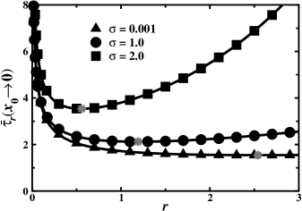
Figure 6: The MTA $\overline{\tau}_{r}$ (the mean first-passage time) versus the resetting rate $r$ for different values of the parameter $\sigma$. The points marked by circles, squares and triangles are outcomes obtained in two stages of computations consisting of the numerical integration performed in Eq. (59) followed by the insertion of the resulting data into Eq. (55). The solid lines represent the exact analytical results given by Eqs. (58), (64) and (65). The grey stars indicate the locci where MTA attains the minimum value. The fixed values of the diffusion coefficient $D\!=\!1.0$ and the initial position $x_{0}\!=\!1.0$ of a diffusing particle have been assumed.

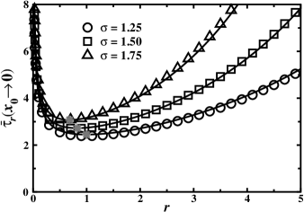
Figure 7: The MTA $\overline{\tau}_{r}$ (the mean first-passage time) versus the resetting rate $r$ for different values of the parameter $\sigma$ falling in the range from $1.0$ to $2.0$. The points marked by circles, squares and triangles are outcomes obtained in two stages of computations consisting of the numerical integration performed in Eq. (59) followed by the insertion of the resulting data into Eq. (55). The solid lines represent the approximate analytical result shown in Eq. (66). The grey stars indicate the locci where MTA attains the minimum value. The fixed values of the diffusion coefficient $D\!=\!1.0$ and the initial position $x_{0}\!=\!1.0$ of a diffusing particle have been assumed.

A propensity of the MTA to be infinite substantially changes when the non-linear diffusion occurs under the influence of exponential resets. To show this effect we can proceed in two equivalent ways. According to the first way it is enough to substitute the Laplace transform of the survival probability (see Eq. (54) with $s\!=\!r$ obtained, respectively, form Eq. (60) for $\sigma\!=\!1$, Eq. (61) for $\sigma\!=\!2$ and (62) for $1\!<\!\sigma\!<\!2$ (see also Eq. (63)) into Eq. (48). In the second case we simply insert the Laplace transforms of PDF given by Eqs. (60), (61) and (62) into the formula derived in Eq. (55). The final results read

$$\overline{\tau}_{r}(x_{0}\!\rightarrow\!0)=\frac{1}{r}\left[\frac{\Gamma\left(\frac{2}{3}\right)}{\Gamma\left(\frac{2}{3},\frac{2\mid x_{0}\mid^{3}}{9D}r\right)+\left(\frac{2r}{9D}\right)^{\frac{2}{3}}x_{0}^{2}\,\mathrm{Ei}\left(-\frac{2\mid x_{0}\mid^{3}}{9D}r\right)}-1\right],$$ (64)

for the parameter $\sigma\!=\!1$,

$$\overline{\tau}_{r}(x_{0}\!\rightarrow\!0)=\frac{1}{r}\left\{\frac{16\left(\frac{D}{r}\right)^{\frac{3}{4}}\exp\left(\frac{\pi^{2}x_{0}}{32D}r\right)}{\sqrt{\pi}\mid\!x_{0}\!\mid^{3}\Gamma\left(\frac{1}{4}\right)\left[\mathrm{K}_{\frac{3}{4}}\left(\frac{\pi^{2}x_{0}}{32D}r\right)-\mathrm{K}_{\frac{3}{4}}\left(\frac{\pi^{2}x_{0}}{32D}r\right)\right]}-1\right\},$$ (65)

for the parameter $\sigma\!=\!2$, and

$$\overline{\tau}_{r}(x_{0}\!\rightarrow\!0)\simeq\frac{1}{r}\left\{\frac{\Gamma\left(\frac{\sigma+1}{\sigma+2}\right)}{\Gamma\left(\frac{\sigma+1}{\sigma+2},\frac{r}{D}\eta(x_{0},\sigma)\right)}\left[1-\left(\frac{r}{D}\eta(x_{0},\sigma)\right)^{\frac{2}{\sigma+2}}\frac{\Gamma\left(\frac{\sigma-1}{\sigma+2},\frac{r}{D}\eta(x_{0},\sigma)\right)}{\Gamma\left(\frac{\sigma+1}{\sigma+2},\frac{r}{D}\eta(x_{0},\sigma)\right)}\right]^{-\frac{1}{\sigma}}-1\right\},$$ (66)

for the parameter $\sigma$ in the range between $1.0$ and $2.0$, where the auxiliary function $\eta(x_{0},\sigma)\!=\!(\sqrt{\mathcal{B}(\sigma)}\mid\!x_{0}\!\mid)^{\sigma+2}$. Dependencies of the MTA $\overline{\tau}_{r}(x_{0}\!\rightarrow\!0)$ on the resetting rate $r$ described by Eqs. (58), (64) and (65) are drawn in Fig. 6 in the form of solid lines. For comparison all the points collected on this plot symbolize the data obtained firstly form numerical integration conducted in Eq. (59) for $\sigma\!=\!0.001$, $1.0$ and $2.0$ and next entered as the input data into Eq. (55). The agreement of these results confirms the numerical procedure we have used to compute MTA works without blemish. The same relations expressed by the approximate Eq. (66) for disparate values of the parameter $\sigma\!=\!1.25$, $1.5$ and $1.75$ are shown in Fig. 7. Note that in both graphs the MTA diverges as $r\!\to\!0$ which retrieves the well-known result that the mean first-passage time to reach the origin tends to infinity when a particle diffuses on the semi-infinite interval in the absence of resetting. On the other hand, the MTA also diverges as $r\!\to\!\infty$, because as the resetting rate increases the diffusing particle does not have enough time, i.e. it has less time between resets, to reach the origin. Therefore, we infer form the behavior of the MTA as a function of $r$ shown in Figs. 6 and 7 that there exists an optimal rate $r_{\ast}$ that minimizes this function. To determine its value we have to solve the following equation, $\left(\frac{\mathrm{d}\overline{\tau}_{r}}{\mathrm{d}r}\right)_{r\!=\!r_{\ast}}\!=\!0$, starting from determination of the first derivative of the MTA with respect to the resetting rate. While this is not too difficult task for Eq. (58), it becomes more complex for the rest of formulae given by Eqs. (64), (65) and (66). Therefore, instead conducting analytical calculations in order to find the optimal resetting rate $r_{\ast}$ we have solved this problem numerically. The values of $r_{\ast}$ for which MTA attains the minimum are distinguished in Figs. 6 and 7 by grey asterisks. Figure 8 presents how the optimal resetting rate $r_{\ast}$ depends on the parameter $\sigma$ for various distances $x_{0}$ from the initial position to the target localized at the origin of the semi-infinite interval (a) and the very distance $x_{0}$ for selected values of the parameter $\sigma$ (b). In both cases the monotonic decrease of $r_{\ast}$ with increase of $x_{0}$ and $\sigma$ is observed such as for the scaled Brownian motion [32].

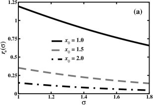
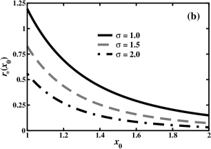
Figure 8: The optimal resetting rate $r_{\ast}$ versus the parameter $\sigma$ (a) and the distance $x_{0}$ to the target (absorbing point) located at the origin of a semi-infinite interval. In both cases we have assumed the fixed value of the diffusion coefficient $D\!=\!1.0$.

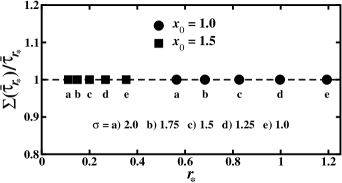
Figure 9: Relative fluctuation in the MTA (the mean first-passage time) versus the optimal resetting rate for different values of the parameter $\sigma$ and two chosen distances $1.0$ and $1.5$ from the initial position $x_{0}$ to the target located at the origin $x\!=\!0$ of the semi-infinite interval. The collected numerical results confirm the assertion expressed in Eq. (67). Here, we have assumed the fixed value of the diffusion coefficient $D\!=\!1.0$.

One of outstanding results concerning any random process intermittent by the exponential resetting is that the relative fluctuation in the MTA, or the mean first-passage time, of an optimally restarted process is always unity [64]. To be more specific, if the resetting rate $r\!=\!r_{\ast}$, i.e. it is equal to the optimal resetting rate, then the relative standard deviation in the MTA satisfies

$$\frac{\Sigma(\overline{\tau}_{r_{\ast}})}{\overline{\tau}_{r_{\ast}}}=1,$$ (67)

and this relation has been proven to be universal. Here, the quantity $\Sigma(\overline{\tau}_{r})\!=\!\sqrt{\,\overline{\tau^{2}_{r}}-\overline{\tau}_{r}^{2}}$ is the standard deviation of the mean first-passage time and $\overline{\tau^{2}_{r}}\!=\!-2\left[\frac{\mathrm{d}\tilde{Q}_{r}(s\,\mid\,x_{0})}{\mathrm{d}s}\right]_{s=0}$ defines its second moment. In this formula the Laplace transform of the survival probability $\tilde{Q}_{r}(s\mid x_{0})$ is determined in Eq. (46). So, the natural question arises whether the relation in Eq. (55) is also satisfied for the non-linear diffusion with the exponential resetting. To give answer to this specific question we proceed as follows. Let us recall the Laplace transform of the survival probability for the non-linear diffusion in the absence of resetting is contained in Eq. (61). By virtue of the second moment of the MTA including exponential restarts along with Eq. (46) we get that

$$\overline{\tau^{2}_{r}}(x_{0}\to 0)=-\frac{2\left[\frac{\mathrm{d}}{\mathrm{d}s}\tilde{Q}(s\!\mid\!x_{0})\right]_{s=r}}{[1-r\tilde{Q}(r\!\mid\!x_{0})]^{2}}.$$ (68)

Combining the above formula with the MTA in Eq. (48) and its squared counterpart we easily calculate the relative standard deviation of the MTA, which is as follows:

$$\frac{\Sigma(\overline{\tau}_{r})}{\overline{\tau}_{r}}=\sqrt{-\bigg{(}\frac{2\frac{\mathrm{d}}{\mathrm{d}s}\tilde{Q}(s\!\mid\!x_{0})\!\mid_{s=r}}{\tilde{Q}^{\,2}(r\!\mid\!x_{0})}+1\bigg{)}}.$$ (69)

In the last step we could insert the survival probability defined by Eq. (43) into this formula and check out validity of the proposition expressed in Eq. (66). Nevertheless, we will proceed in another way because the resulting formula is too complex and the optimal resetting rates $r_{\ast}$ can only be determined by means of a numerical procedure. Thus, we firstly determine their values for a few exemplary values of the parameter $\sigma$ and different distances from the initial position $x_{0}$ to the origin of the semi-infinite interval. Then, by performing numerical computations on the basis of Eqs. (61) and (68) we find the ratio $\Sigma(\overline{\tau}_{r_{\ast}})/\overline{\tau}_{r_{\ast}}$. The plot shown in Fig. 9 illustrates the final results and confirm correctness of the theorem in Eq. (67) for non-linear diffusion with the exponential resetting.

5 Conclusions

Despite evident differences between the free linear and non-linear diffusion, there exists one common property connecting the both processes, that is, inability to reach the non-equilibrium steady state. This situation dramatically changes when a particle executing a diffusive motion undergoes the action of a permanent external force driving a system out of equilibrium. In this paper we examined the alternative mechanism that enables a diffusing particle to be in the stationary state. Instead of the force a system is subject to resetting, a kind of stochastic process in which some moving object is turned back at random moments of time to a given initial state, from where it starts its motion anew. Since the first publication considering this problem [15], a lot of papers have appeared in recent years on different variants of diffusion models with stochastic resetting. To our best knowledge all of them were dedicated to study a numerous variety of the linear diffusion equations. Being motivated by this fact we have decided to explore probably not yet studied effect of stochastic resetting on the non-linear diffusion. In the present paper we have restricted our attention exclusively to the simplest, canonical version of the exponential (Poissonian) resetting. Thereby, we save a detailed analysis of the other schemes of stochastic resetting, interesting from theoretical and experimental points of view, for the future work.

The summary of the present work is as follows. At the beginning we have invoked a specific form of the non-linear differential equation in which the diffusion coefficient depends on the probability density through the power-law function. Next, we have briefly described the effective method of how to solve this type of a differential equation and then commented its general solution. Getting a minimal experience in this subject has allowed us to examine how the Poissonian resetting affects the basic properties of the non-linear diffusion. It turned out that unlike ordinary diffusion the MSD for the non-linear diffusion firstly increases with time to finally achieve the constant value over much longer time scales. Such a behavior of the MSD indicates that also the time-dependent PDF should attain under the influence of stochastic resetting a permanent profile in the steady state. Indeed, we have found such stationary distributions in the form of two exact results that refer to peculiar values of the power-law exponent $\sigma\!=\!1$ and $2$, and the approximate formula when the values of the parameter $\sigma$ fall into the range between $1$ and $2$. In order to obtain this last expression we have used the algebraic approximation consisting in a replacement of the integrand in Eq. (28) with the power-law function arising from the Taylor expansion. We have also tested the second approach based on the exponential approximation and derived the alternative formula for the stationary PDF. In this case, the PDF depends on the position of a diffusing particle according to the stretched exponential tail $p_{r}(x)\!\simeq\!\exp\left(-\eta x^{\frac{2(\sigma+2)}{\sigma+4}}\right)$ for large $x$. We have demonstrated that if $\sigma\!\to\!0$ the complete form of the PDF boils down to the two-sided exponential probability density that results from a solution of the linear diffusion equation extended with additional terms accounting for exponential resets [15]. However, in contrast to the PDF for the linear diffusion the spatial domain of the PDF for the non-linear diffusion is restricted to a confined support outside of which this function disappears. Our studies have shown that the mechanism of exponential resetting extends this finite support of the PDF to the entire domain of real numbers.

In this paper, we have also analysed the process of non-linear diffusion with the Poissonian resetting from a perspective of its first-passage properties. To that end we assumed the system with a totally absorbing barrier (the target) placed at the origin of the semi-infinite interval and an initial position of a diffusing particle at a distant point. As the main result we have derived the exact and approximate expressions for the mean time to absorption (the mean first-passage time). This quantity has been studied as the function of the resetting rate and different values of the parameter $\sigma$. The conclusion emerging from these studies is that the exponential resetting makes the mean time towards the absorbing point to be finite and even the shortest one for a particular value of the resetting rate. This means the mean time needed for a diffusing particle to reach a target attains the global minimum for a given optimal resetting rate $r_{\ast}$. Furthermore, we have shown that $r_{\ast}$ decreases with the increase of a distance between an initial position $x_{0}$ and the target. A dependence of $r_{\ast}$ on and the power-law exponent $\sigma$ displays a similar monotonic decrease. Finally, we have tested and confirmed the universal property that the relative fluctuation in the mean first-passage time of optimally restarted non-linear diffusion intermittent by exponential resetting is equal to unity.

The present paper constitutes only a prelude to more advanced investigations of non-linear processes evolving under a given dynamics disturbed by stochastic resetting. In particular, it will be interesting to analyse the non-linear diffusion in a presence of external potentials, under the influence of non-exponential resetting protocols, under non-instantaneous returns and explore the temporal relaxation of this process to the stationary state, to name but a few research directions. We are hopeful that the present work will initiate a new route for theoretical and experimental studies of stochastic resetting in the context of various non-linear phenomena.

Appendix

The goal of this supplementary section is to present the formal derivation of Eq. (32) included in the main text. Setting the parameter $\sigma\!=\!2$ we get from Eqs. (7) and 8 that two numerical factors appearing in Eq. (28) take the following values, $\mathcal{A}(2)\!=\!\frac{1}{\sqrt{\pi}}$ and $\mathcal{B}(2)\!=\!\frac{\pi}{4}$. In addition, the auxiliary function in this equation is $\xi(x,2)\!=\!\left(\frac{\pi}{4}\right)^{2}\frac{(x-x_{0})^{4}}{D}$. Thus, inserting all these quantities into Eq. (28) we obtain

$$p_{r}(x\!\mid\!x_{0})=\frac{r}{\sqrt{\pi}}\bigintsss_{\xi(x,2)}^{\infty}\frac{\mathrm{e}^{-rt}}{(Dt)^{\frac{1}{4}}}\sqrt{1-\frac{\pi(x-x_{0})^{2}}{4\sqrt{Dt}}}\,\mathrm{d}t.$$ (A.1)

Now, upon introducing the new notation $a(x)\!\equiv\!\sqrt{\xi(x,2)}$ and changing the variable of integration from $t$ to $\tau$, so that $t\!=\!(\tau^{2}+a(x))^{2}$, we can transform the PDF in Eq. (A.1) into the much simpler form:

$$p_{r}(x\!\mid\!x_{0})=\frac{4r}{\sqrt{\pi\sqrt{D}}}\int_{0}^{\infty}\tau^{2}\exp\left[-r(\tau^{2}+a(x))^{2}\right]\,\mathrm{d}\tau.$$ (A.2)

From now on the rest of our calculations boils down to the solution of the above integral. It can be find by using the similarly looking integral [90]

$$\int_{0}^{\infty}\exp\left(-\alpha\tau^{4}-2\beta\tau^{2}\right)\mathrm{d}\tau=\frac{1}{2}\sqrt{\frac{\beta}{2\alpha}}\exp\left(\frac{\beta^{2}}{2\alpha}\right)\mathrm{K}_{\frac{1}{4}}\left(\frac{\beta^{2}}{2\alpha}\right),$$ (A.3)

where the both factors $\alpha$, $\beta\!>\!0$ and $\mathrm{K}_{\nu}(z)$ is the modified Bessel function of the second kind. Out of many well-known properties of this function we utilize the two ones:

$$\mathrm{K}_{\nu}(z)=\mathrm{K}_{-\nu}(z),$$ (A.4)

and

$$\frac{\mathrm{d}}{\mathrm{d}z}\mathrm{K}_{\nu}(z)=-\mathrm{K}_{\nu-1}(z)-\frac{\nu}{z}\mathrm{K}_{\nu}(z).$$ (A.5)

At first, however, let us differentiate both sides of Eq. (A.3) with respect to the parameter $\beta$. In this way, we have

$$\int_{0}^{\infty}\tau^{2}\exp\left(-\alpha\tau^{4}-2\beta\tau^{2}\right)\mathrm{d}\tau=-\frac{1}{4\sqrt{2\alpha}}\frac{\mathrm{d}}{\mathrm{d}\beta}\left[\sqrt{\beta}\exp\left(\frac{\beta^{2}}{2\alpha}\right)\mathrm{K}_{\frac{1}{4}}\left(\frac{\beta^{2}}{2\alpha}\right)\right].$$ (A.6)

Taking into account Eqs. (A.4) and (A.5) we show that a derivative of the expression enclosed in the square bracket on the right hand side of the above equation

$$\frac{\mathrm{d}}{\mathrm{d}\beta}\left[\sqrt{\beta}\exp\left(\frac{\beta^{2}}{2\alpha}\right)\mathrm{K}_{\frac{1}{4}}\left(\frac{\beta^{2}}{2\alpha}\right)\right]=\frac{\beta\sqrt{\beta}}{\alpha}\exp\left(\frac{\beta^{2}}{2\alpha}\right)\left[\mathrm{K}_{\frac{1}{4}}\left(\frac{\beta^{2}}{2\alpha}\right)-\mathrm{K}_{\frac{3}{4}}\left(\frac{\beta^{2}}{2\alpha}\right)\right].$$ (A.7)

If we plug this derivative back into Eq. (A.6) and multiply their both sides by the exponential function $\exp(-\frac{\beta^{2}}{\alpha})$, we obtain that the integral

$$\bigintsss_{0}^{\infty}\tau^{2}\exp\left[-\alpha\left(\tau^{2}+\frac{\beta}{\alpha}\right)^{2}\right]\mathrm{d}\tau=\frac{1}{4\sqrt{2}}\left(\frac{\beta}{\alpha}\right)^{\frac{3}{2}}\exp\left(-\frac{\beta^{2}}{2\alpha}\right)\left[\mathrm{K}_{\frac{3}{4}}\left(\frac{\beta^{2}}{2\alpha}\right)-\mathrm{K}_{\frac{1}{4}}\left(\frac{\beta^{2}}{2\alpha}\right)\right].$$ (A.8)

Having this equation at our disposal and taking $\alpha\!=\!r$ and $\beta\!=\!ra(x)$, we immediately find out the integral in Eq. (A.2) and hence the exact formula expressing the PDF with the parameter $\sigma\!=\!2$ for the non-linear diffusion intermittent by exponential resets. The final result is as follows

$$p_{r}(x\!\mid\!x_{0})=\frac{ra^{\frac{3}{2}}(x)}{\sqrt{2\pi\sqrt{D}}}\exp\!\left(-\frac{ra^{2}(x)}{2}\right)\left[\mathrm{K}_{\frac{3}{4}}\!\left(\frac{ra^{2}(x)}{2}\right)-\mathrm{K}_{\frac{1}{4}}\!\left(\frac{ra^{2}(x)}{2}\right)\right],$$ (A.9)

where the variable $a(x)\!=\!\frac{\pi(x-x_{0})^{2}}{4\sqrt{D}}$.

To complete this supplement we should also determine the value of the PDF for $x\!=\!x_{0}$. It can be done in two ways. The first method takes advantage of the following limit values of the modified Bessel functions of the second kind:

$$\lim_{z\to 0}z^{3}\mathrm{K}_{\frac{1}{4}}\left(uz^{4}\right)=0,$$ (A.10)

and

$$\lim_{z\to 0}z^{3}\mathrm{K}_{\frac{3}{4}}\left(uz^{4}\right)=\frac{\Gamma\left(\frac{3}{4}\right)}{\sqrt[4]{2}\,u^{3/4}}.$$ (A.11)

Calculating these limits in Eq. (A.9) we easily show that

$$p_{r}(x_{0})=\frac{\Gamma\left(\frac{3}{4}\right)}{\sqrt{\pi}}\left(\frac{r}{D}\right)^{\frac{1}{4}}.$$ (A.12)

The second method that guarantees the above result consists in the direct calculation of the integral in Eq. (A.2) for $x\!=\!x_{0}$ with $\xi(x_{0},2)\!=\!0$. In this case we use the integral representation of the Euler gamma function, i.e. $\Gamma(\alpha)\!=\!\int_{0}^{\infty}u^{\alpha-1}\mathrm{e}^{-u}\mathrm{d}u$.

Conflicts of Interest

The author declares no conflict of interest.

References

- [1] M. Magoni, S. N Majumdar, and G. Schehr. Ising model with stochastic resetting. Phys. Rev. Research, 2:033182, 2020.
- [2] J. Fuchs, S. Goldt, and U. Seifert. Stochastic thermodynamics of resetting. EPL, 113:60009, 2016.
- [3] A. Pal and S. Rahav. Integral fluctuations theorems for stochastic resetting systems. Phys. Rev. E, 96:062135, 2017.
- [4] D. Gupta, C. A. Plata, and A. Pal. Work fluctuations and jarzynski equality in stochastic resetting. Phys. Rev. Lett., 124:110608, 2020.
- [5] E. Roldan, A. Lisica, D. Sanches-Taltavull, and S. W. Grill. Stochastic resetting in backtrack recovery by rna polymerases. Phys. Rev. E, 96:062411, 2016.
- [6] S. Budnar and et al. Anillin promotes cell contractility by cyclic resetting of rhoa residence kinetics. Dev. Cell, 49:894–906, 2019.
- [7] S. Reuveni, M. Urbakh, and J. Klafter. Role of substrate unbinding in michaelis-menten enzymatic reactions. Proc. Natl. Acad. Sci. U. S. A., 111:4391, 2014.
- [8] T. Rotbart, S. Reuveni, and M. Urbakh. Michaelis-menten reaction scheme as a unified approach towards the optimal restart problem. Phys. Rev. E, 92:060101, 2015.
- [9] A. Pal, L. Kuśmierz, and S. Reuveni. Search with home returns provides advantage under high uncertainty. Phys. Rev. Research, 2:043174, 2020.
- [10] H. Tong, C. Faloutsos, and J-Y. Pan. Random walk with restart: fast solutions and applications. Knowl. Inf. Syst., 14:327, 2008.
- [11] K. Avrachenkov, A. Piunovskiy, and Y. Zhang. Markov processes with restart. J. Appl. Probab., 50:960, 2013.
- [12] S. Janson and Y. Peres. Hitting times for random walks with restarts. SIAM J. Discrete Math., 26:537, 2012.
- [13] K. Avrachenkov, A. Piunovskiy, and Y. Zhang. Hitting times in markov chains with restart and their application to network centrality. Methodol. Comput. Appl. Probab., 20:1173, 2018.
- [14] M. R. Evans, S. N. Majumdar, and G. Schehr. Stochastic resetting and applications. J. Phys. A: Math. Theor., 53:193001, 2020.
- [15] M. R. Evans and S. N. Majumdar. Diffusion with stochastic resetting. Phys. Rev. Lett., 106:160601, 2011.
- [16] M. R. Evans and S. N. Majumdar. Diffusion with optimal resetting. J. Phys. A: Math. Theor., 44:435001, 2011.
- [17] C. Christou and A. Schadschneider. Diffusion with resetting in bounded domains. J. Phys. A: Math. Theor., 48:285003, 2015.
- [18] A. Chatterjee, C. Christou, and A. Schadschneider. Diffusion with resetting inside a circle. Phys. Rev. E, 97:062106, 2018.
- [19] A. Pal. Diffusion in a potential landscape with stochastic resetting. Phys. Rev. E, 91:012113, 2015.
- [20] É. Roldan and S. Gupta. Path-integral formalism for stochastic resetting: exactly solved examples and shortcuts to confinement. Phys. Rev. E, 96:022130, 2017.
- [21] S. Ray. Space-dependent diffusion with stochastic resetting: A first-passage study. J. Chem. Phys., 153:234904, 2020.
- [22] M. R. Evans and S. N. Majumdar. Diffusion with resetting in arbitrary spatial dimension. J. Phys. A: Math. Theor., 47:285001, 2014.
- [23] J. Whitehouse, M. R. Evans, and S. N. Majumdar. Effect of partial absorption on diffusion with resetting. Phys. Rev. E, 87:022118, 2013.
- [24] R. Falcao and M. R. Evans. Interacting brownian motion with resetting. J. Stat. Mech., page 023204, 2017.
- [25] U. Basu, A. Kundu, and A. Pal. Symmetric exclusion process under stochastic resetting. Phys. Rev. E, 100:032136, 2019.
- [26] A. Masó-Puigdellosas, D. Campos, and V. Méndez. Anomalous diffusion in random-walks with memory-induced relocations. AIP Conf. Proc., 7:112, 2019.
- [27] J. Masoliver and M. Montero. Anomalous diffusion under stochastic resetting: a general approach. Phys. Rev. E, 100:042103, 2019.
- [28] L. Kusmierz, S. N. Majumdar, S. Sabhapandit, and G. Schehr. First order transition for the optimal search time of levy flights with resetting. Phys. Rev. Lett., 113:220602, 2014.
- [29] Ł. Kuśmierz and E. Gudowska-Nowak. Optimal first-arrival times in levy flights with resetting. Phys. Rev. E, 92:052127, 2015.
- [30] D. Gupta. Stochastic resetting in underdamped brownian motion. J. Stat. Mech., page 033212, 2019.
- [31] A. S. Bodrova, A. V. Chechkin, and I. M. Sokolov. Nonrenewal resetting of scaled brownian motion. Phys. Rev. E, 100:012119, 2015.
- [32] A. S. Bodrova, A. V. Chechkin, and I. M. Sokolov. Scaled brownian motion with renewal resetting. Phys. Rev. E, 100:012120, 2015.
- [33] W. Wang, A. G. Cherstvy, H. Kantz, R. Metzler, and I. M. Sokolov. Time averaging and emerging nonergodicity upon resetting of fractional Brownian motion and heterogeneous diffusion processes. Phys. Rev. E, 104:024105, 2021.
- [34] D. Campos and V. Méndez. Phase transitions in optimal search times: how random walkers should combine resetting and flight scales. Phys. Rev. E, 92:062115, 2015.
- [35] S. N. Majumdar, S. Sabhapandit, and G. Schehr. Random walk with random resetting to the maximum position. Phys. Rev. E, 92:052126, 2015.
- [36] M. Montero and J. Villarroel. Directed random walk with random restarts: the sisyphus random walk. Phys. Rev. E, 94:032132, 2016.
- [37] V. Méndez and D. Campos. Characterization of stationary states in random walks with stochastic resetting. Phys. Rev. E, 93:022106, 2016.
- [38] L. N. Christophorov. Peculiarities of random walks with resetting in a one-dimensional chain. J. Phys. A 54:015001, 2021.
- [39] M. Montero and J. Villarroel. Monotonous continuous-time random walks with drift and stochastic reset events. Phys. Rev. E, 87:012116, 2013.
- [40] M. Montero, A. Masó-Puigdellosas, and J. Villarroel. Continuous-time random walks with reset events: historical background and new perspectives. Eur. Phys. J. B, 90:176, 2017.
- [41] Ł. Kuśmierz and E. Gudowska-Nowak. Subdiffusive continuous-time random walks with stochastic resetting. Phys. Rev. E, 99:052116, 2019.
- [42] J. Masoliver. Telegraphic processes with stochastic resetting. Phys. Rev. E, 99:012121, 2019.
- [43] D. Campos and V. Méndez. Characterization of stationary states in random walks with stochastic resetting. Phys. Rev. E, 93:022106, 2016.
- [44] A. Pal, R. Chatterjee, S. Reuveni, and A. Kundu. Local time of diffusion with stochastic resetting. J. Phys. A: Math. Theor., 52:264002, 2019.
- [45] J. M.. Meylahn, S. Sabhapandit, and H. Touchette. Large deviations for markov processes with resetting. Phys. Rev. E, 92:062148, 2015.
- [46] U. Bhat, C. De Bacco, and S. Redner. Stochastic search with poisson and deterministic resetting. J. Stat. Mech., page 083401, 2016.
- [47] M. A. F. dos Santos. Fractional prabhakar derivative in diffusion equation with non-static stochastic resetting. Physics, 1:40, 2019.
- [48] Ł. Kuśmierz and T. Toyoizumi. Robust random search with scale-free stochastic resetting. Phys. Rev. E, 100:032110, 2019.
- [49] S. Eule and J. J. Metzger. Non-equilibrium steady states of stochastic processes with intermittent resetting. New. J. Phys., 18:033006, 2016.
- [50] D. Boyer, M. R. Evans, and S. N. Majumdar. Long time scaling behaviour for diffusion with resetting and memory. J. Stat. Mech., page 023208, 2017.
- [51] A. Pal, A. Kundu, and M. R. Evans. Diffusion under time-dependent resetting. J. Phys. A: Math. Theor., 49:225001, 2016.
- [52] A. Nagar and S. Gupta. Diffusion with stochastic resetting at power-law times. Phys. Rev. E, 93:060102(R), 2016.
- [53] O. Tel-Friedman, A. Pal, A. Sekhon, S. Reuveni, and Y. Roichman. Experimental realization of diffusion with stochastic resetting. J. Phys. Chem. Lett., 11:7350–5, 2020.
- [54] B. Besga, A. Bovon, A. Petrosyan, S. N. Majumdar, and S. Ciliberto. Optimal mean first-passage time for a brownian searcher subjected to resetting: experimental and theoretical results. Phys. Rev. Res., 2:032029(R), 2020.
- [55] A. Pal, Ł. Kuśmierz, and S. Reuveni. Search with home returns provides advantage under high uncertainty. Phys. Rev. Res., 2:043174, 2020.
- [56] A. Pal, Ł. Kuśmierz, and S. Reuveni. Invariants of motion with stochastic resetting and space-time coupled returns. New. J. Phys., 21:113024, 2019.
- [57] A. Pal, Ł. Kuśmierz, and S. Reuveni. Time-dependent density of diffusion with stochastic resetting is invariant to return speed. Phys. Rev. E, 100:040101, 2019.
- [58] A. Maso-Puigdellosas, D. Campos, and V. Mendez. Transport properties of random walks under stochastic noninstantaneous resetting. Phys. Rev. E, 100:042104, 2019.
- [59] A. S. Bodrova and I. M. Sokolov. Resetting processes with noninstantaneous return. Phys. Rev. E, 101:052130, 2020.
- [60] A. S. Bodrova and I. M. Sokolov. Brownian motion under noninstantaneous resetting in higher dimensions. Phys. Rev. E, 102:032129, 2020.
- [61] M. R. Evans and S. N. Majumdar. Effects of refractory period on stochastic resetting. J. Phys. A: Math. Theor., 52:01LT01, 2018.
- [62] D. Gupta, C. A. Plata, A. Kundu, and A. Pal. Stochastic resetting with stochastic returns using external trap. J. Phys. A: Math. Theor., 54:025003, 2021.
- [63] D. Gupta, A. Pal, and A. Kundu. Resetting with stochastic return through linear confining potential. J. Stat. Mech., page 043202, 2021.
- [64] S. Reuveni. Optimal stochastic restart renders fluctuations in first passage times universal. Phys. Rev. Lett., 116:170601, 2016.
- [65] A. Pal and S. Reuveni. First passage under restart. Phys. Rev. Lett., 118:030603, 2017.
- [66] A. Chechkin and I. M. Sokolov. Random search with resetting: a unified renewal approach. Phys. Rev. Lett., 121:050601, 2018.
- [67] O. Bénichou, M. Coppey, M. Moreau, P-H Suet, and R. Voituriez. Optimal search strategies for hidden targets. Phys. Rev. Lett., 94:198101, 2005.
- [68] M. R. Evans, S. N. Majumdar, and K. Mallick. Optimal diffusive search: nonequilibrium resetting versus equilibrium dynamics. J. Phys. A: Math. Theor., 46:185001, 2013.
- [69] F. Bartumeus and J. Catalan. Optimal search behaviour and classic foraging theory. J. Phys. A: Math. Theor., 42:434002, 2009.
- [70] J. Snider. Optimal random search for a single hidden target. Phys. Rev. E, 83:011105, 2012.
- [71] Ł. Kuśmierz and E. Gudowska-Nowak. Optimal first-arrival times in levy flights with resetting. Phys. Rev. E, 92:052127, 2015.
- [72] A. Montanari and R. Zecchina. Optimizing searches via rare events. Phys. Rev. Lett., 88:178701, 2002.
- [73] S. Redner. A guide to first-passage processes. Cambridge University Press, 2001.
- [74] S. Ahmad, I. Nayak, A. Bansal, A. Nandi, and D. Das. First-passage of a particle i a potential under stochastic resetting: a vanishing transition of optimal resetting rate. Phys. Rev. E, 99:022130, 2019.
- [75] Ł. Kuśmierz, M. Bier, and E. Gudowska-Nowak. Optimal potentials for diffusive search strategies. J. Phys. A: Math. Theor., 50:185003, 2017.
- [76] X. Durang, S. Lee, L. Lizana, and J-H Jeon. First-passage statistics under stochastic resetting in bounded domains. J. Phys. A: Math. Theor., 52:224001, 2019.
- [77] A. Pal and V. V. Prasad. First passage under stochastic resetting in an interval. Phys. Rev. E, 99:033123, 2019.
- [78] A. Pal, I. Eliazar, and S. Reuvenu. First passage under restart with branching. Phys. Rev. Lett., 122:020602, 2019.
- [79] A. Ray, A. Pal, D. Ghosh, S. K. Dana, and C. Hens. Mitigating long transient time in deterministic systems by resetting. Chaos, 31:011103, 2021.
- [80] L. Debnath. Nonlinear partial differential equations for scientists and engineers. Birkhäuser, 2012.
- [81] A. Fasano and M. Primicerio. (Eds.) Nonlinear diffusion problems. Springer-Verlag, 1986.
- [82] J. L. Vázquez. The porous medium equation. Oxford University Press, 2007.
- [83] G. I. Barenblatt, V. M Entov, and V. M. Ryzhik. Theory of fluid flows through natural rocks. Dordrecht, Netherlands: Kluver, 1990.
- [84] J. G. Berryman and C. J. Holland. Nonlinear diffusion problem arising in plasma physics. Phys. Rev. Lett., 40:1720–1722, 1978.
- [85] P. Ya. Polubarinova-Kochina. On a nonlinear differential equation encountered in the theory of infiltration. Dokl. Acad. Nauk SSSR, 63:623–627, 1948.
- [86] M. E. Gurtin and R. C. MacCamy. On the diffusion of biological populations. Math. Biosci., 33:35–49, 1977.
- [87] J. D. Murray. Mathematical Biology, I. An Introduction. Springer, 2002.
- [88] I. C. Christov and H. A. Stone. Resolving a paradox of anomalous scalings in the diffusion of granular materials. Proc. Natl. Acad. Sci. USA, 109:16012–7, 2012.
- [89] D. Pritchard, A. W. Woods, and A. J. Hogg. On the slow draining of a gravity current moving through a layered permeable medium. J. Fluid Mech., 444:23–47, 2001.
- [90] I. S. Gradshteyn and I. M. Ryzhik. Table of Integrals, Series, and Products. Elsevier Inc., 2007.
- [91] Ya. B. Zel’dovich and G. I. Barenblatt. The asymptotic properties of self-modelling solutions of the nonstationary gas filtration equations. Sov. Phys. Doklady, 3:44–47, 1958.
- [92] E. Pattle, R. Diffusion from an instantaneous point source with concentration dependent coefficient. Quart. J. Mech. Appl. Math., 12:407–409, 1959.
- [93] G. I. Barenblatt and Ya. B. Zel’dovich. Self-similar solutions as intermediate asymptotics. Ann. Rev. Fluid Mech., 4:285–312, 1972.
- [94] D. R. Cox. Renewal Theory. John Wiley&Sons, 1962.
- [95] R. Wong. Asymptotic Approximations of Integrals. SIAM, 2001.
- [96] J. L. Schiff. The Laplace Transform. Theory and Applications. Springer, 1999.
- [97] J. Wang, W-J. Zhang, J-R. Liang, J-B. Xiao, and F-Y. Ren. Fractional nonlinear diffusion equation and first passage time. Physica A, 387:764–772, 2008.