Localization and delocalization properties in quasi-periodically perturbed Kicked Harper and Harper models

Abstract

We numerically study the single particle localization and delocalization phenomena of an initially localized wave packet in the kicked Harper model (KHM) and Harper model subjected to quasi-periodic perturbation composed of $M-$modes. Both models are localized in the monochromatically perturbed case $M=1$. KHM shows localization-delocalization transition (LDT) above $M\geq 2$ as increase of the perturbation strength $\epsilon$. In contrast, in a time-continuous Harper model with the perturbation, it is confirmed that the localization persists for $M=2$ and the LDT occurs for $M\geq 3$. Furthermore, we investigate the diffusive property of the delocalized wave packet in the KHM and Harper model for $\epsilon$ above the critical strength $\epsilon_{c}$ ($\epsilon>\epsilon_{c}$) comparing with other type systems without localization, which takes place a ballistic to diffusive transition in the wave packet dynamics as the increase of $\epsilon$.

I Introduction

The quantum kicked rotor (KR), representing the dynamics of a periodically kicked pendulum, is a well studied as example of a classically nonintegrable system casati79 ; fishman82 ; reichl04 . The dynamical localization of the quantum KR has been interpreted through a mapping to the Anderson tight-binding model for a particle in a disordered lattice fishman82 . Furthermore, in the KR systems, a transition from the dynamical localization to delocalization can be caused by second periodic series of kicks, and periodic modulation of the kick amplitude, and so on abal02 ; wang08 ; schomerus08 .

Similar to the KR systems, the existence of localization-delocalization transition (LDT) in the dynamics has been investigated in the kicked Harper model (KHM), whose classical counterpart is a non-integrable system biddle09 ; molina14 ; rayanov15 ; ganeshan15 ; major18 ; castro19 ; alexAn21 . There are three types of main dynamical states of the quantum wave packet, localized, normal diffusion, and ballistic spread, corresponding to the change of the potential strength in the KHM. In that respect, it is the same as the Harper model without the kicks. In the case of the Harper model, at one point of the potential strength, the LDT takes place due to the duality of the system harper55 ; hofstadter76 ; aubry80 . On the other hand, the phase diagram of the localized/delocalized state in KHM has a nested structure and is quite complicated artuso94 ; prosen01 ; kolovsky03 ; levi04 . In the case of KHM, there is also studies on the LDT caused by the second kick series or kick intensity modulation kolovsky12 ; wang13 ; qin14 ; cadez17 ; ravindranath21 ; lakshminarayan03 ; mishra16 ; ray18 .

In general, for the periodically driven Hamiltonian systems, Floquet states represent the natural generalization of the stationary eigenstates for time-independent systems. Floquet engineering in the periodically kicked systems is interesting because they can exhibit more complex dynamics and the quantum state is more controllable through external driving in comparison to their static systems kolovsky12 ; wang13 ; qin14 ; cadez17 ; ravindranath21 ; lakshminarayan03 ; mishra16 ; ray18 .

Recently, the LDT by using the KR has been experimentally explored using cold atoms in optical lattices sadgrove07 ; dana08 ; chabe08 ; lemarie10 . It is also feasible to experimentally realize the dynamical LDT through the diffusion of wave packets in the pulsed 1D incommensurate optical lattice such as the KHM sarkar17 .

On the other hand, we have also investigated the characteristics of the LDT in the polychromatically perturbed kicked Anderson model (KAM), and the results that correspond well with those in the KR have been obtained yamada04 ; yamada10 ; yamada15 ; yamada18 ; yamada20 ; yamada20a . [ Note that in our previous paper, we used the expression Anderson map (AM) for the KAM. ] The dynamics is not solely determined by the strength $\epsilon$ of the perturbation, but also the number of color $M$ of the coherent perturbation. It was shown that for the time-continuous 1D Anderson model modulated by a quasi-periodic time-perturbation of $M$ colors, if there are three or more color perturbations ($M\geq 3$), the Anderson localized states without the perturbation can be delocalized, and the LDT occurs as the increase of $\epsilon$ yamada21 ; yamada22 .

In this work, we study the dynamical LDT in the KHM and Harper models which are perturbed by the quasi-periodic oscillations. Specifically, in the KHM of $2\leq M<\infty$, there are LDTs and the characteristics are similar to those of the KAM. However, in the Harper model, the case of $M=2$ is completely localized on the small side of $\epsilon$, and tends to persist the localization and the LDT has not been observed even on the large side of $\epsilon$. In the time-continuous Harper model with the polychromatic perturbation, the LDT does not occur in the case of $M=2$, and the LDT occurs only in a case of $M\geq 3$, as seen in the case of the 1D Anderson model with the polychromatic perturbation yamada21 ; yamada22 .

It should be noticed that the persistence of the localization for $1\leq M<\infty$ is mathematically claimed in the regime of weak enough dynamical perturbations and strong disorder potential Soffer03 ; Bourgain04 ; hatami16 . In this regard, the present paper reports the details of novel results on dynamical delocalization in the perturbed Harper model. Of particular interest to us is dependence of the LDT on the two parameters of coherent polychromatic perturbation, i.e., number of the colors $M$ and perturbation strength $\epsilon$.

Furthermore, by using the other type system without localization, which is related to both the KHM and Harper models, we report the change in the wave packet dynamics from the ballistic spreading in the unperturbed Bloch state to the normal diffusion when the perturbation strength is increased. Hereinafter, this transition is referred to as a ballistic-diffusive transition (BDT) of wave packet spreading. The timescale for the BDT depends on the strength $\epsilon$ as well as $M$. In the next section, those indicating BDT are introduced as B-type system. In contrast, those indicating LDT are used as A-type system.

In Sec.II we introduce the model and the basic property. Section III explores the dynamical LDT when perturbed by quasi-periodic oscillation with the component $M$ and the strength $\epsilon$. In contrast, in Sect.IV, we focus on the diffusive property of the delocalized states, and show the relation to BDT by the coherent perturbation in the B-type system. In Sect.V, the relationship of the diffusive states in the A-type and B-type systems is shown. In the last section, we summarize our findings while comparing them with other results.

II Models and some preliminaries

We deal with the dynamically perturbed kicked Harper model (KHM),

$$H_{kick}(t) = \sum\limits_{n=1}^{N}{|n\rangle V(n)[L+f_{\epsilon}(t)]\langle n|}\delta_{1}(t)$$ (1)

$$+ T\sum\limits_{n}^{N}({|n\rangle\langle n+1|+|n+1\rangle\langle n|}),$$

where $\delta_{1}(t)=\sum_{m\in{\mathbb{Z}}}\delta(t-m)$. The on-site energy sequence is

$$V(n)=2V\cos(2\pi Qn),$$ (2)

where $\{|n\rangle\}$ is an orthonormalized basis set and the $Q$ is an irrational number. $V$ is potential strength, and $T$ denotes the hopping energy between adjacent sites, respectively. We tale $Q=\frac{\sqrt{5}-1}{2}$ and $T=-1$ throughout the present paper.

The coherently time-dependent part $f_{\epsilon}(t)$ is given as,

$$f_{\epsilon}(t)=\epsilon f(t)=\frac{\epsilon}{\sqrt{M}}\sum_{i}^{M}\cos(\omega_{i}t+\theta_{i}),$$ (3)

where $M$ and $\epsilon$ are the number of frequency components and the strength of the perturbation, respectively. Note that the long-time average of the total power of the perturbation is normalized to $\overline{f_{\epsilon}(t)^{2}}=\epsilon^{2}/2$ and $\{\theta_{i}\}$ are the initial phases. Since we see the long-time behavior regardless of how the initial phases are taken, we basically set it as $\{\theta_{i}=0\}$, but we also partially deal with the case of random phases. The frequencies $\{\omega_{i}\}(i=1,...,M)$ are taken as mutually incommensurate numbers of order $O(1)$. Following two types of cases:

$$\begin{cases}L=1&({\rm A-type~{}system})\\ L=0&({\rm B-type~{}system}).\end{cases}$$ (4)

behave completely differently to the perturbation. In the A-type system the LDT occurs by increasing of the perturbation strength $\epsilon$. Even in the B-type system the normal diffusion occurs by increasing of $\epsilon$ through the BDT.

For the initial wave packet $<n|\Psi(t=0)>=\delta_{n,n_{0}}$ localized at the site $n_{0}$, we calculate the time evolution of the wavefunction $|\Psi(t)>$ using Schrodinger equation:

$$i\hbar\frac{\partial|\Psi(t)>}{\partial t}=H(t)|\Psi(t)>.$$ (5)

We monitor the spread of the wave function in the site space by the mean square displacement (MSD),

$$m_{2}(t)=\sum_{n}(n-n_{0})^{2}\left<|\phi(n,t)|^{2}\right>,$$ (6)

where $\phi(n,t)=<n|\Psi(t)>$ is the site representation of the wave function.

In the numerical simulation for the time-continuous system, we used 2nd order symplectic integrator with time step $\Delta t=0.02\sim 0.05$. The number of steps is $10^{5}\sim 10^{7}$. We mainly use the system size $N=2^{14}-2^{16}$, and $\hbar=1/8$ for KHM, and $\hbar=1$ and $\hbar=1/8$ for Harper model.

The unperturbed KHM ($\epsilon=0$) is known to take a localized, critical, and extended state with a change of $V$. Figure 1 shows the time-deprendence of the MSD $m_{2}(t)$ when the potential strength $V$ is changed from the localized side to the delocalized one. In all cases, the $m_{2}(t)$ grows $m_{2}\sim t^{2}$ for small $t$, but the behavior for $t>>1$ is quite different with the parameter $V$. If $V$ is small, we can see ballistic spreading $m_{2}\sim t^{2}$. When $V=1$, normal diffusive behavior close to $m_{2}\sim t^{1}$ is observed, and when $V$ is large, it tends to be localized. However, the $V-$dependence in the KHM is considerably more complicated than the unperturbed Harper model introduced below as a time-continuous system. Indeed, even if it is localized, the $V-$dependence of the localization length cannot be simply given diffrent from the case of Harper model. In the corresponding classical dynamics, the unperturbed KHM shows chaos, but the unperturbed Harper model is an integrable system in a classical limit. The eigenvalue problem of the periodically kicked system can be replaced with the eigenvalue problem of the tight-binding system by the Maryland transform. As given in Appendix A, one can easily check that the eigenvalue problem of the quantum map system interacting with $M$-color modes can be transformed into $d(=M+1)$-dimensional lattice problem with disorder by Maryland transform. Without loss of generality, mainly for a fixed value $V=5$ to be localized we investigate the LDT in the A-type systems with increasing of $M$ and $\epsilon$ of the quasi-periodic perturbation in the next section.

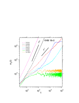
Figure 1: (Color online) The double logarithmic plots of $m_{2}$ as a function of $t$ for some values of the potential strength $V=0.4,0.8,1.0,2.5,3.0,5.0,10.0$ in the unperturbed A-type KHM ($\epsilon=0$). $\hbar=1/8$. The solid lines have slope 1 and 2.

Furthermore, we examine the LDT for a time-continuous system in which $\delta_{1}(t)$ is replaced by 1 in the Hamiltonian $H_{kick}(t)$. This model was introduced as an model for electron in a two-dimensional crystal in an external magnetic field, and we call it Harper model in this paper. [There are also references that describes this model as Aubry-Andre model or Aubry-Andre-Harper model. ] It can be said that the KHM system is a map version of the Harper model.

The nature of the unperturbed Harper model ($\epsilon=0$) has long been well studied physically and mathematically. It has been also shown that the LDT exists in the unpertubed Harper model due to the duality hiramoto88 ; geisel91 ; wilkinson94 . For $V>1$ all eigenstates are localized and the spectrum is pure point. For $V>1$ the localization length $\xi$ is given $\xi=\frac{1}{\log V}$ independent on the energy. In this case, the increase in $V$ causes a monotonous decrease in $\xi$. For $V<1$ the states are extended and the spectrum is absolutely continuous. For the critical value $V=V_{c}=1$ eigenstates are critical and the spectrum is singular continuous. It is also numerically suggested that spread of an initially localized wavepacket is localized for $V>1$, and is ballistic for $V<1$ and is diffusive for $V=1$, respectively math-comment .

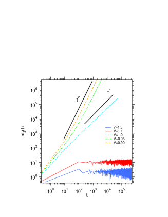
Figure 2: (Color online) The double logarithmic plots of $m_{2}$ as a function of $t$ for some values of the potential strength $V=1.3,1.05,1.0,0.95,0.9$ in the unperturbed A-type Harper model ($\epsilon=0$). $\hbar=1$. The solid lines have slope 1 and 2.

Figure 2 shows the MSD in the unperturbed Harper model when the potential strength $V$ is changed from the localized side ($V>1$) to the delocalized side ($V<1$). Although there are fluctuations, it changes from $m_{2}\sim t^{0}$ in the case of localization to a ballistic spread of $m_{2}\sim t^{2}$ via normal diffusive behavior $m_{2}\sim t^{1}$ in the case of the critical state ($V=1$). When $V<1$, it is ballistic regardless of the value of $V$. That is,

$$m_{2}(t)\sim\begin{cases}t^{0}{\rm(localization)}&V>1\\ t^{1}{\rm(normal~{}diffusion)}&V=V_{c}=1\\ t^{2}{\rm(ballistic~{}spreading)}&V<1\end{cases}$$ (7)

Using the A-type Harper model, we fixed at $V=1.3$ as an unperturbed localized side, and investigate the LDT by imposing $f_{\epsilon}(t)$, with comparing with results in the already reported 1D kicked Anderson and the Anderson models yamada20a ; yamada21 ; yamada22 .

In general, anomalous diffusion $m_{2}(t)\sim t^{\alpha}$ characterized by diffusion index $\alpha$ is expected for the LDT ($0<\alpha<1$) and BDT ($1<\alpha<2$). The instantaneous diffusion index $\alpha_{ins}(t)$ is also used to directly investigate the existence of the LDT and the BDT:

$$\alpha_{ins}(t)=\frac{d\log m_{2}(t)}{d\log t}.$$ (8)

In the A-type system, above the critical point $\epsilon>\epsilon_{c}$ the index becomes unity ($\alpha=1$) indicating the normal diffusion, and for $\epsilon<\epsilon_{c}$ it decreases to zero ($\alpha=0$) indicating localization. Around the critical point $\epsilon\simeq\epsilon_{c}$ for LDT $\alpha_{ins}(t)\simeq\alpha_{c}(<1)$ for $t>>1$. In the B-type system, above $\epsilon>\epsilon_{b}$ the $\alpha(t)$ becomes unity, and for $\epsilon<\epsilon_{b}$ it increases to 2 indicating the ballistic spreading.

III Dynamical Localization-Delocalization Transition

In this section, we examine the dynamical property by changing the parameters $M$ and $\epsilon$ of the perturbation $f_{\epsilon}(t)$ in the A-type system of the KHM with $V=5$ and Harper model with $V=1.3$, respectively.

III.1 Kicked Harper model: A-type case

Figure 3(a) shows the time-dependence of MSD in the log-log plots when $M=1$. When $\epsilon$ is small, it is clearly completely localized. Even when $\epsilon$ increases, it spreads diffusively within the initial time, but as time elapses, the $t-$linear growth begins to wither and the wave packet tends to be localized. As a result, no transition to the delocalized state is seen in the monochromatically perturbed case.

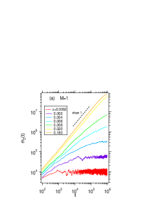
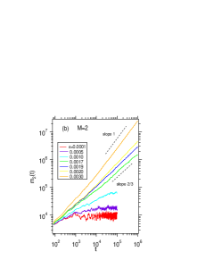
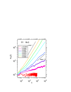
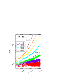
Figure 3: (Color online) The double-logarithmic plots of $m_{2}(t)$ as a function of time for different values of the perturbation strength $\epsilon$ in the polychromatically perturbed A-type KHM of $V=5$ with (a)$M=1$, (b)$M=2$, (c)$M=3$, (d)$M=7$. $\hbar=1/8$. The values of $\epsilon$ used are $\epsilon=0.0002,0.0020,0.0040,0.0080,0.0200,0.1800$ from bottom to top in the panel (a), $\epsilon=0.0001,0.0005,0.0010,0.0017,0.0019,0.0020,0.0030$ from bottom to top in the panel (b), $\epsilon=0.0001,0.0005,0.0007,0.0009,0.0012,0.0015,0.0020$ from bottom to top in the panel (c), and $\epsilon=0.0001,0.0002,0.00028,0.0004,0.0005,0.0006$ from bottom to top in the panel (b), respectively. The dashed lines have slope 1 in the panel (a), slope 1 and 2/3 in the panel (b), slope 1 and 1/2 in the panel (c), and slope 1 and 1/4 in the panel (d), respectively.

In Fig.3(b)(c)(d), the MSD are shown for $M\geq 2$. They are localized when $\epsilon$ is small, but the LDT occurs with a certain critical value $\epsilon_{c}$, and $\epsilon$ becomes larger than $\epsilon_{c}$, warps upward (upward deviation) can be seen in the double-logarithmic plots. For $\epsilon>\epsilon_{c}$ the normal diffusive behavior $m_{2}\sim t^{1}$ appears as $t\to\infty$.

As shown in Fig.3(b)(c)(d), around $\epsilon=\epsilon_{c}$ the time-dependence of MSD can be approximately described by the sub-diffusive spreading

$$m_{2}(t)\sim t^{\alpha},\alpha\simeq\frac{2}{M+1},$$ (9)

depending on $M$.

As shown in Fig.4, for $M\geq 2$ the $M-$dependence of the critical strength $\epsilon_{c}$ indicates the inverse power-law

$$\epsilon_{c}\propto\frac{1}{V}\frac{1}{(M-1)}.$$ (10)

The same $M-$dependence even for $V=10$ can be obtained, as seen in Fig.4. This difference in $\epsilon_{c}$ due to $V$ can be interpreted by the Maryland transform in Appendix A. According to the Maryland transform, the effect of $V$ in the diagonal term is saturated in the region $V>V^{*}(\equiv 0.38)$, and the nature of the off-diagonal term depends on $\epsilon V$, so the critical value $\epsilon_{c}$ for $V=10$ can be interpreted as a half of the critical value $\epsilon_{c}$ of the transition point for $V=5$.

It can also be seen that for $\epsilon>\epsilon_{c}$, $m_{2}(t)$ asymptotically becomes to normal diffusion as $t\to\infty$. Therefore, we can say that the quasi-periodically driven system also may delocalize even in the absence of coupling with its environment.

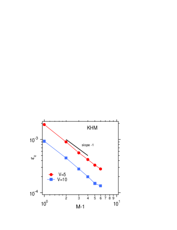
Figure 4: (Color online) The critical perturbation strength $\epsilon_{c}$ as a function of $(M-1)$ for A-type KHM with $V=5$ and $V=10$. The black solid line shows $\epsilon_{c}\propto 1/(M-1)$.

Using $\alpha_{ins}(t)$, we confirm the above LDT trend. As shown in Fig.5, in the case of KHM, we can see that with an increase of $\epsilon$ the tendency of $\alpha_{int}\to 0$ changes as $\alpha_{int}\to 1$ through $\alpha_{int}(t)=\alpha_{c}\simeq 2/(M+1)$ around $\epsilon\simeq\epsilon_{c}$ for $t>>1$.

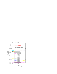
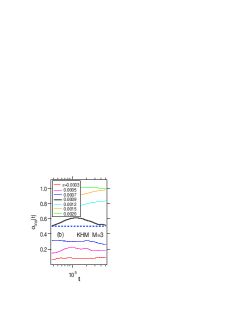
Figure 5: (Color online) The time-dependence of $\alpha_{ins}(t)$ for various strength $\epsilon$ in the perturbed A-type KHM of $V=5$ with (a)$M=2$ and (b)$M=3$. $\hbar=1/8$. The values of $\epsilon$ used are $\epsilon=0.001,0.0016,0.0017,0.0018,0.0019,0.002,0.003,0.004$ from top to bottom in the panle (a), and $\epsilon=0.0003,0.0005,0.0007,0.0009,0.0012,0.0015,0.0020$ from top to bottom in the panle (b), respectively. The dotted lines indicate $\alpha=2/(M+1)$.

III.2 Harper model: A-type case

Is the LDT as seen in the perturbed KHM observed when using the Harper model? The potential strength is fixed at $V=1.3$, and the time-dependence of the MSD for the cases of $M=1$ and $M=2$ is shown in Fig.6. Obviously, if $\epsilon$ is small, it is localized, and the localization persists even for $\epsilon\sim 0.6$ beyond the region that can be regarded as a perturbation. It is completely localized in the sense that $D=\frac{m_{2}}{t}\to 0$ can be guessed. Also for $M=2$, at least clear subdiffusion does not appear even if $\epsilon$ is increased to $\epsilon\geq 0.65$. (See Fig.6(b).) As a result, it also tends to be localized even for $M=2$, which is also the same as the result for the 1D Anderson model with a random sequence as $V(n)$ yamada22 .

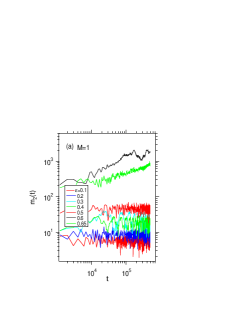
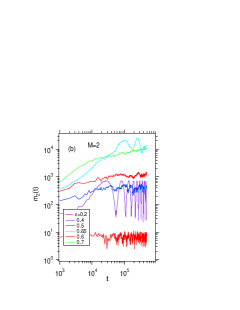
Figure 6: (Color online) The double logarithmic plots of $m_{2}$ as a function of $t$ for some values of the perturbation strength $\epsilon$ in the perturbed A-type Harper model of the potential strength $V=1.3$. (a)$M=1$ and (b)$M=2$. $\hbar=1$. The values of $\epsilon$ used are $\epsilon=0.1,0.2,0.3,0.4,0.5,0.6,0.65$ from bootom to top in the panel (a) and $\epsilon=0.2,0.4,0.5,0.6,0.65,0.7$ from bootom to top in the panel (b), respectively.

Figure 7 shows the result of $m_{2}(t)$ for $M\geq 3$ when $\epsilon$ is increased. First, the results for $M=3$ with different parameters are given in Fig.7(a) and (b). As seen in Fig.7(a), it is clearly localized in the region $\epsilon<0.5$, but it changes for $\epsilon>0.7$, and appears to be asymptotic to diffusive one ($m_{2}\sim t^{1}$). Figure 7(b) is the result by using the random initial phases $\{\theta_{i}\}$ of $f_{\epsilon}(t)$. It is a similar result to the Fig.7(a). If $\epsilon$ is small, it is localized, but if $\epsilon\sim 0.5$, the fluctuation becomes large, and if $\epsilon>0.65$, it becomes diffusive $m_{2}\sim t^{1}$. As a result, in the perturbed A-type Harper model of $M=3$, we can see a transition from a localized to a delocalized dynamics takes place through subdiffusion $m_{2}\sim t^{2/3}$ around the critical value $\epsilon_{c}\simeq 0.5$.

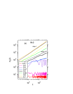
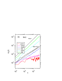
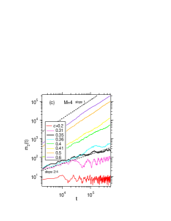
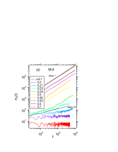
Figure 7: (Color online) The double logarithmic plots of $m_{2}$ as a function of $t$ for some values of the perturbation strength $\epsilon$ in the perturbed A-type Harper model of the potential strength $V=1.3$ with (a)$M=3$,$\{\theta_{i}\}_{0}$, (b)$M=3$, $\{\theta_{i}\}_{random}$, (c)$M=4$, $\{\theta_{i}\}_{0}$, (d)$M=5$, $\{\theta_{i}\}_{0}$. $\hbar=1$. The values of $\epsilon$ used are $\epsilon=0.1,0.2,0.4,0.47,0.5,0.55,0.6,0.7$ from bottom to top in the panel (a), $\epsilon=0.4,0.45,0.48,0.5,0.55,0.6$ from bottom to top in the panel (b), $\epsilon=0.2,0.31,0.35,0.36,0.4,0.41,0.5,0.6$ from bottom to top in the panel (c), and $\epsilon=0.1,0.2,0.21,0.23,0.24,0.3,0.35,0.42,0.5,0.7$ from bottom to top in the panel (b), respectively. $\{\theta_{i}\}_{0}$ maens to take all phases to zero, and $\{\theta_{i}\}_{random}$ means that random phases are selected. The dashed lines have slope 1 and 2/3 in the panel (a) and (b), slope 1 and 2/4 in the panel (c), and slope 1 and 2/5 in the panel (d), respectively.

Figure 7(c) and (d) show the result of $M=4$ and $M=5$, respectively. It is also seen that the change from the localized state to the normal diffusion as in the case of $M=3$. In the case of $M=4$, it is clearly localized for $\epsilon<0.3$, and it becomes diffusive at least for $\epsilon>0.4$. In the case of $M=5$, it is clearly localized for $\epsilon<0.2$, and it becomes diffusive at least for $\epsilon>0.4$.

From the whole, the transition point $\epsilon_{c}$ tends to decrease with $M$. However, unlike the case of the KHM, a clear subdiffusion ($m_{2}\sim t^{\alpha}$, $0<\alpha<1$) cannot be detected during the transition from the localized ($m_{2}\sim t^{0}$) to delocalized ($m_{2}\sim t^{1}$) dynamical property by increasing $\epsilon$. The overall tendency corresponds well to the case of KAM and Anderson model where $V(n)$ is random sequence.

The above trends can be seen on the behavior of $\alpha_{ins}(t)$. As shown in Fig.8, for the Harper model the transition from $\alpha\to 0$ to $\alpha\to 1$ exists with increasing $\epsilon$, but it is difficult to obtain a stable subdiffusion with $\alpha=2/M$ or $\alpha=2/(M+1)$ in the process.

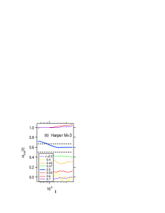
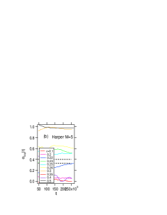
Figure 8: (Color online) The time-dependence of $\alpha_{ins}(t)$ for various strength $\epsilon$ in the perturbed A-type Harper model of $V=1$ with (a)$M=3$ and (b)$M=5$. $\hbar=1$. The values of $\epsilon$ used are $\epsilon=0.20,0.40,0.45,0.47,0.50,0.55,0.60,0.70$ from top to bottom in the panel (a), and $\epsilon=0.1,0.2,0.23,0.25,0.26,0.3,0.35,0.4,0.5$ from top to bottom in the panel (b), respectively. The dotted lines indicate $\alpha=2/M$ and $\alpha=2/(M+1)$.

IV Transition from ballistic spreading to normal diffusion

In this section, we study the characteristics of the wave packet spreading in the B-type KHM and Harper model ($L=0$) with the coherent oscillation $f_{\epsilon}(t)$. If $\epsilon=0$, the potential term disappears, so both KHM and Harper model are periodic systems, and the localized wave packet spreads ballistically:

$$m_{2}(t)\sim t^{2}.$$ (11)

In appendix A for the KHM, we can also see that the diagonal term in the Maryland transformed tight-binding model does not depend on the site $n$, so it becomes a ballistic motion. In the B-type cases, $V$ and $\epsilon$ play the same role, so basically fix it as $V=1$ and we investigate the wave packet dynamics while changing $M$ and $\epsilon$ of the coherent oscillation part.

IV.1 Kicked Harper model: B-type case

In the case of the B-type KHM with $M=1$ and $M=5$, the time-dependence of MSD is given in Fig.9. In both cases, when $\epsilon$ is small, the growth of $m_{2}(t)$ slightly deviates from ballistic spreading at the initial time, but it goes to ballistic as $t\to\infty$. It can be seen that when $\epsilon$ becomes large, it gradually approaches normal diffusion, $m_{2}(t)\sim t^{1}$, from the initial stage. That is, even if $M\geq 1$, there is a transition from ballistic to normal diffusion, Unlike the LDT case in the previous section, there is no theoretical guide based on Anderson transition, so the superdiffusion at the BDT must be captured numerically. This will be shown at another time yamada22a . The asymptotic diffusive behavior is expected as a generic feature of decoherence, which takes place when noise is introduced into the system.

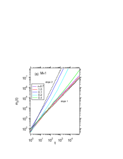
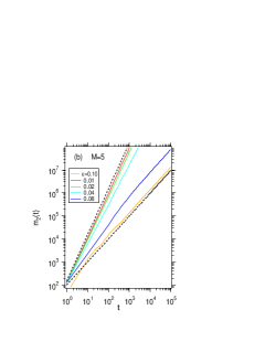
Figure 9: (Color online) The double-logarithmic plots of $m_{2}(t)$ as a function of $t$ for various strength $\epsilon$ in the B-type perturbed KHM of $V=1$ with (a)$M=1$ and (b)$M=5$. $\hbar=1/8$. The values of $\epsilon$ used are $\epsilon=0.1,0.2,0.4,0.7,1.0$ from top to bottom in the panel (a), and $\epsilon=0.01,0.02,0.04,0.08,0.10$ from top to bottom in the panel (b), respectively. The dashed lines indicate normal diffusion $m_{2}\propto t^{1}$ and ballistic spreading $m_{2}\propto t^{2}$

We confirme this by the behavior of $\alpha_{ins}(t)$ used in the LDT in the previous section. As seen in Fig.10, both for M=1 and M=5. A transition from $\alpha\to 2$ to $\alpha\to 1$ is suggested when $\epsilon$ increases, although it is also difficult to accurately determine the value of $\epsilon_{b}$ for the transition.

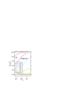
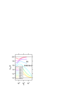
Figure 10: (Color online) The time-dependence of $\alpha_{ins}(t)$ for various strength $\epsilon$ in the B-type perturbed KHM of $V=1$ with (a)$M=1$ and (b)$M=5$. $\hbar=1/8$. The values of $\epsilon$ used are $\epsilon=0.1,0.2,0.3,0.4,0.5,0.7,0.9,1.0$ from top to bottom in the panel (a), and $\epsilon=0.01,0.02,0.03,0.04,0.05,0.06,0.07,0.08$ from top to bottom in the panel (b), respectively. The dotted lines indicate $\alpha=1$ and $\alpha=2$.

IV.2 Harper model: B-type case

In the case of the B-type Harper model, the time-dependence of MSD for some $\epsilon$ is given in Fig.11. When $M=1$ in the Fig.11(a), it shifts to the normal diffusion side at the initial time, but in the all cases, we can see that the increase in $m_{2}(t)$ is parallel to the line with slope 2 as $t\to\infty$. On the other hand, as shown in Fig.11(b)-(d) for $M\geq 2$, at short time scale, the wave-packet spread is ballistic, but for larger time scale the spread becomes diffusive. This is a typical feature of approaching the BDT around the critical point $\epsilon_{b}$. The system transits from ballistic into asymptotic normal diffusive regime. Again, let us confirm the features by using $\alpha_{ins}(t)$. We can observe the transition from $\alpha\to 2$ to $\alpha\to 1$ for the case of $M=3$ in Fig.12.

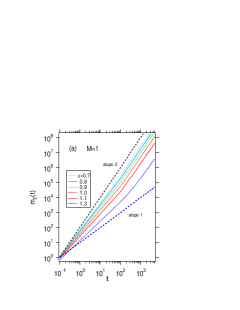
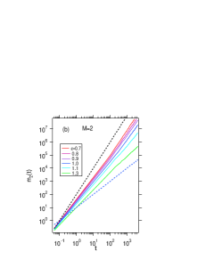
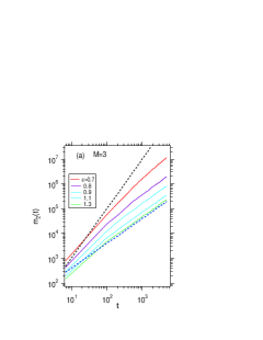
Figure 11: (Color online) The double-logarithmic plots of $m_{2}(t)$ as a function of $t$ for various strength $\epsilon=0.7,0.8,0.9,1.1,1.3$ from top to bottom, in the B-type perturbed Harper model of $V=1$ with (a)$M=1$, (b)$M=2$, (c)$M=3$ and (d)$M=5$. $\hbar=1/8$. The dashed lines indicate normal diffusion $m_{2}\sim t^{1}$ and ballistic spreading $m_{2}\sim t^{2}$.

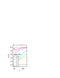
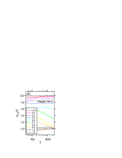
Figure 12: (Color online) The time-dependence of $\alpha_{ins}(t)$ for various strength $\epsilon$ in the B-type perturbed Harper model of $V=1$ with (a)$M=1$ and (b)$M=3$. $\hbar=1/8$. The values of $\epsilon$ used are $\epsilon=0.9,1.0,1.1,1.3,1.4,1.5,1.6,1.7$ from top to bottom in the panel (a), and $\epsilon=0.2,0.3,0.4,0.5,0.6,0.7,0.8,1.0,1.3$ from top to bottom in the panel (b), respectively. The dotted lines indicate $\alpha=1$ and $\alpha=2$.

V The delocalized states in A-type and B-type systems

It is easy to imagine that the A-type system asymptotically approaches the B-type system with the increase of $\epsilon$, because the time-dependent part of the Hamiltonian (1) can be rewritten:

$$\epsilon V(n)\left[\frac{L}{\epsilon}+f(t)\right]\delta_{1}(t).$$ (12)

As seen in the last section, even in the case of B-type system, the time-dependence of MSD shows the normal diffusion for $\epsilon>\epsilon_{b}$ and the diffusion coefficient decreases by increasing $\epsilon$. On the other hand, as seen in the previous section, even in the A-type system, for $\epsilon>\epsilon_{c}$, $m_{2}(t)$ gradually approaches the normal diffusion for $t\to\infty$. In this section, we give the relationship between the results of the diffusive region in the A-type and B-type systems. Here, in the KHM the $\epsilon-$dependence of the diffusion coefficient in the normal diffusive regime in a wide region of $\epsilon$($>\max\{\epsilon_{c},\epsilon_{b}\}$) is observed in Fig.13.

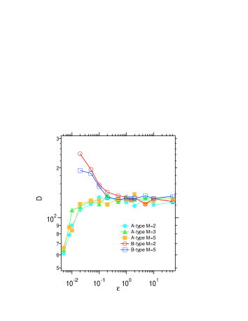
Figure 13: (Color online) Diffusion coefficient $D$ as a function of $\epsilon$ in the A-type and B-type perturbed KHM of $V=5$.$\hbar=1/8$. Note that the both axes are in logarithmic scale.

In the A-type system, the diffusion coefficient increases with an increase of $\epsilon$ when $\epsilon>\epsilon_{c}$ and the effect saturates at a certain level. On the other hand, in B-type system, the diffusion coefficient decreases monotonically as $\epsilon$ increases, and it can be seen that $D$ falls to the same level as A-type system for $\epsilon>>1$. For $\epsilon>0.3$, $M-$dependence of the diffusion coefficient has almost disappeared for the both systems.

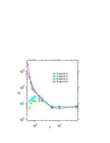
Figure 14: (Color online) Diffusion coefficient $D$ as a function of $\epsilon$ in the A-type and B-type perturbed Harper model of $V=1.3$.$\hbar=1/8$. Note that the both axes are in logarithmic scale.

Furthermore, as shown in Fig.14, similar results are obtained for the A-type and B-type systems of the time-continuous Harper model. In this case, in A-type system, increasing $\epsilon$ also increases $D$ and peaks around $\epsilon\simeq 1$ then decreases, and approaches the same constant level as B-type system for large $\epsilon$.

VI Summary and discussion

In the present paper, we investigated the dynamical property of the initially localized wave packet in coherently perturbed kicked Harper and Harper models.

In the A-type systems ($L=1$), localization-delocalization transition (LDT) appeared with increasing the perturbation strength $\epsilon$. The critical value $M_{c}$ which appear the LDT is $M_{c}=2$ for KHM, and $M_{c}=3$ for Harper model. The property for the number of the color $M$ is summarized in table 1. The table also describes the LDT in the multidimensional Anderson model that corresponds to the 1D Anderson map and Anderson model with the quasiperiodic perturbation. In the case of KHM, if $M+1$ can be identified with the spatial dimension $d$, the existence of the LDT is a qualitatively consistent result with those of the LDT in $d-$dimensional Anderson model anderson58 ; abrahams79 ; lifshiz88 ; abrahams10 . However, in the time-continuous systems, the critical number of the colors, degrees of freedom, is not $d=M+1=2$ but $d=3$, unlike the periodically kicked quantum maps such as KAM and KHM notarnicola18 ; tarquini17 . We hope that this study will be useful for studying the long-time behavior of the dynamics in high-dimensional random systems and multi-degree-of-freedom quantum systems that cannot be calculated directly. Our results suggest that in a general localized systems, there is a transition point $\epsilon_{c}$ of the perturbation strength corresponding to the number of color $M$ of the quasi-periodic perturbation, and there are characteristic critical dynamics at the point. It controls the quantum coherence that causes the localization.

In the B-type systems ($L=0$) of the KHM and Harper model, the sharp ballistic-diffusive transition (BDT) of the dynamics of the wave-packet can be observed with the increase of the strength $\epsilon$. The dynamical motion depends on the number of the color $M$. The result is summarized in table 2. In this case, no localized state occurs, but it may be more realistic in terms of investigating how the scattering of the one-particle problem changes due to the addition of coherent perturbations to the periodic system of $\epsilon=0$. Furthermore, it was shown that in both the KHM and Harper model, the A-type system becomes one equivalent to the B-type system in the normal diffusion region of $\epsilon>>1$. The asymptotic diffusive behavior is expected as a generic feature of decoherence, which takes place when noise is introduced into a system.

This work may lead to a deeper understanding of dynamical localization and quantum diffusion in quasi-periodic systems. It also provides insight into the control of localized and delocalized states by coherent perturbations in the Floquet engineering.

Table 1: $M-$dependence of the DLT in the A-type KHM and Harper model. For $4\leq M<\infty$ the result is same as the case of $M=3$. Those in the kicked Anderson and Anderson model are also entered for reference. The lower lines is a result of the $d-$dimensional disordered systems. Loc: exponential localization, Diff:Normal diffusion.

$M$	0	1	2	3	4
Anderson model yamada21	Loc	Loc	Loc	LDT	LDT
Harper model($V>1$)	Loc	Loc	Loc	LDT	LDT
Kicked Anderson model yamada20	Loc	Loc	LDT	LDT	LDT
Kicked rotor yamada20	Loc	Loc	LDT	LDT	LDT
Kicked Harper model ($V>>1$)	Loc	Loc	LDT	LDT	LDT
d	d=1	d=2	d=3	d=4	d=5
$d-$D Anderson model	Loc	Loc	LDT	LDT	LDT

Table 2: $M-$dependence of the BDT in the B-type KHM and Harper model. For $3\leq M<\infty$ the result is same as the case of $M=2$. Balli:Ballistic propagation, Loc: exponential localization, Diff:Normal diffusion.

$M$	0	1	2	3	4
Anderson model yamada21	Balli	Loc	Diff	Diff	Diff
Harper model ($V>1$)	Balli	Balli	BDT	BDT	BDT
Kicked Anderson model yamada20a	Balli	Loc	Diff	Diff	Diff
Kicked Harper model ($V>>1$)	Balli	BDT	BDT	BDT	BDT

Appendix A Maryland transform

We can regard the time-dependent harmonic perturbation $f_{\epsilon}(t)$ as the dynamical degrees of freedom. To show this we introduce the classically canonical action-angle operators $(\hat{J}_{j}=-i\hbar\frac{\partial_{j}}{\partial_{j}\phi_{j}},\phi_{j})$ representing the harmonic perturbation as the linear modes, and we call them the color modes. Each quantum oscillator has the action eigenstates $|n_{j}>$ with the action eigenvalue $J_{j}=n_{i}\hbar~{}(n_{j}:$integer) and the energy $n_{j}\hbar\omega_{j}$, where $\hat{J}_{j}|m_{j}\rangle=m_{j}\hbar|m_{j}\rangle$($m_{j}\in{\mathbb{Z}}$). Thus the system (1) is regarded as a quantum system of $(M+1)$-degrees of freedom spanned by the quantum states $|n>\prod_{j=1}^{M}|n_{j}>$. Then the Hamiltonian $\tilde{H}_{kick}$ that include the color modes becomes

$$\tilde{H}_{kick}(\hat{p},\hat{q},\{\hat{J}_{j}\},\{\hat{\phi}_{j}\})=2\cos(\hat{p}/\hbar)+$$

$$2V\cos(2\pi Q\hat{q})\left[L+\frac{\epsilon}{\sqrt{M}}\sum_{j}^{M}\cos\hat{\phi}_{j}\right]\delta_{1}(t)+\sum_{j=1}^{M}\omega_{j}\hat{J}_{j}.$$ (13)

Let us consider an eigenvalue equation

$${\rm e}^{-i\hat{A}}{\rm e}^{-i\hat{B}}{\rm e}^{-i\hat{C}}|u\rangle={\rm e}^{-i\gamma}|u\rangle,$$ (14)

where

$$\begin{cases}\hat{A}=(2VL\cos(2\pi Q\hat{q})+\sum_{j}^{M}\omega_{i}\hat{J}_{j})/\hbar,\\ \hat{B}=\cos(2\pi Q\hat{q})\frac{\epsilon 2V}{\sqrt{M}}\sum_{j}^{M}\cos\hat{\phi}_{j}/\hbar,\\ \hat{C}=2\cos(\hat{p}/\hbar)/\hbar\end{cases}$$ (15)

for the time-evolution operator $T{\rm e}^{-\frac{i}{\hbar}\int\tilde{H}_{kick}dt}$. $\gamma$ and $|u\rangle$ are the quasi-eigenvalue and quasi-eigenstate. Here, if the eigenstate representation of $\hat{J}_{j}$ is used, we can obtain the following $(M+1)-$dimensional tight-binding expression by the Maryland transform yamada20 :

$$D(n,\{m_{j}\})u(n,\{m_{j}\})+$$

$$\sum_{n^{\prime},\{m_{j}^{{}^{\prime}}\}}\langle n,\{m_{j}\}|\hat{t}_{KHM}|n^{\prime},\{m_{j}^{{}^{\prime}}\}\rangle u(n^{\prime},\{m_{j}^{{}^{\prime}}\})=0,$$ (16)

where $\{m_{j}\}=(m_{1},....,m_{M})$. Here the diagonal term is

$$D(n,\{m_{j}\})=\tan\left[\frac{2VL\cos(2\pi Qn)+\hbar\sum_{j}^{M}m_{j}\omega_{j}}{2\hbar}-\frac{\gamma}{2}\right],$$ (17)

and the $\hat{t}_{KHM}$ of the off-diagonal term is

$$\hat{t}_{KHM}=i\frac{e^{-i\frac{\epsilon 2V}{\sqrt{M}}\cos(2\pi Q\hat{q})(\sum_{j}^{M}\cos\hat{\phi}_{j})/\hbar}-e^{i2\cos(\hat{p}/\hbar)/\hbar}}{e^{-i\frac{\epsilon 2V}{\sqrt{M}}\cos(2\pi Q\hat{q})(\sum_{j}^{M}\cos\hat{\phi}_{j})/\hbar}+e^{i2\cos(\hat{p}/\hbar)/\hbar}}.$$ (18)

$D(n,\{m_{j}\})$ is $\epsilon-$independent and the off-diagonal term is $\epsilon-$dependent. It follows that the $(M+1)-$dimensional tight-binding model of the KHM have singularity of the on-site energy caused by tangent function and long-range hopping caused by the kick $\delta_{1}(t)$.

In the cases of the A-type system ($L=1$), there exists $2V^{*}=2\pi\hbar$, that is $V^{*}\simeq 0.38$ for $\hbar=1/8$, where the effect of the the fluctuation width of the diagonal term is saturated for the change of the potential strength $V$ due to the tangent function (17). Therefore, for $V>V^{*}$ the delocalization can be caused by increase of $\epsilon$ in the off-diagonal term in the form of $2\epsilon V$. Note that the transform is not possible in the time-continuous systems such as Harper model.

References

- (1) G. Casati, B. V. Chirikov, F.M. Izraelev, and J. Ford, Stochastic behavior of a quantum pendulum under a periodic perturbation, Lect. Notes Phys. 93, 334 (1979).
- (2) S. Fishman, D. R. Grempel, and R. E. Prange, Chaos, Quantum Recurrences, and Anderson Localization, Phys. Rev. Lett. 49, 509(1982).
- (3) L. Reichl, The Transition to Chaos: Conservative Classical Systems and Quantum Manifestations (Springer Science and Business Media, New York, 2004).
- (4) G. Abal, R. Donangelo, A. Romanelli, A.C. Sicardi Schifino, R. Siri, Dynamical Localization in Quasi-Periodic Driven Systems, Phys. Rev. E 65, 046236 (2002).
- (5) J. Wang, A. M. Garcia-Garcia, Classical and quantum anomalous diffusion in a system of 2 kicked Quantum Rotors, Int. J. Mod. Phys. B 22, 5261 (2008).
- (6) H. Schomerus and E. Lutz, Controlled decoherence in a quantum Lévy kicked rotator, Phys. Rev. A 77, 062113(2008).
- (7) J. Biddle, B. Wang, D. J. Priour Jr., and S. Das Sarma, Localization in one-dimensional incommensurate lattices beyond the Aubry-André model, Phys. Rev. A 80, 021603(R)(2009).
- (8) L. Morales-Molina, E. Doerner, C. Danieli, and S. Flach, Resonant extended states in driven quasiperiodic lattices: Aubry-André localization by design, Phys. Rev. A 90, 043630(2014).
- (9) C.Danieli, K.Rayanov, B.Pavlov, G.Martin, S.Flach, Approximating Metal-Insulator Transitions, Int. J. Mod. Phys. B 29, 1550036(2015).
- (10) S.Ganeshan, J.H. Pixley, and S.D. Sarma, Nearest Neighbor Tight Binding Models with an Exact Mobility Edge in One Dimension, Phys. Rev. Lett. 114, 146601(2015).
- (11) Jan Major, Giovanna Morigi, and Jakub Zakrzewski, Single-particle localization in dynamical potentials, Phys. Rev. A 98, 053633(2018).
- (12) G.A. Domínguez-Castro, R. Paredes, The Aubry–André model as a hobbyhorse for understanding the localization phenomenon, Eur. J. Phys. 40, 045403(2019).
- (13) F. A. An al., Interactions and Mobility Edges: Observing the Generalized Aubry-André Model, Phys. Rev. Lett. 126, 040603(2021).
- (14) P.G. Harper, Single band motion of conduction electrons in a uniform magnetic field, Proc. Phys. Soc. London A 68, 874(1955).
- (15) D.R. Hofstadter, Energy levels and wave functions of Bloch electrons in rational and irrational magnetic fields, Phys. Rev. B 14, 2239 (1976).
- (16) S. Aubry and G. André, Analyticity breaking and Anderson localization in incommensurate lattices, Ann. Isr. Phys. Soc. 3, 18 (1980).
- (17) R. Artuso, G. Casati, F. Borgonovi, L. Rebuzzini and I. Guarneri, Fractal and dynamical properties of the kicked harper model, International Journal of Modern Physics B 8, 207-235 (1994).
- (18) T. Prosen, I. I Satija, N. R. Shah, Dimer Decimation and Intricately Nested Localized-Ballistic Phases of Kicked Harper, Phys.Rev.Lett.87, 066601(2001).
- (19) A. R. Kolovsky and H. J. Korsch, Quantum diffusion in a biased kicked Harper system, Phys. Rev. E 68, 046202(2003).
- (20) B. Lévi and B. Georgeot, Quantum computation of a complex system: The kicked Harper model, Phys. Rev. E 70, 056218(2004).
- (21) A. R. Kolovsky and G. Mantica, The driven Harper model, Phys. Rev. B 86, 054306(2012).
- (22) H. Wang, D.Y. H. Ho, W. Lawton, J. Wang, and J.Gong, Kicked-Harper model versus on-resonance double-kicked rotor model: From spectral difference to topological equivalence, Phys. Rev. E 88, 052920(2013).
- (23) P. Qin, C. Yin, and S. Chen, Dynamical Anderson transition in one-dimensional periodically kicked incommensurate lattices, Phys. Rev. B 90, 054303 (2014).
- (24) T. Cadez, R. Mondaini, and P. D. Sacramento, Dynamical localization and the effects of aperiodicity in Floquet systems, Phys. Rev. B 96,144301 (2017).
- (25) V. Ravindranath and M. S. Santhanam, Dynamical transitions in aperiodically kicked tight-binding models, Phys. Rev. B 103, 134303(2021).
- (26) A. Lakshminarayan and V. Subrahmanyam, Entanglement sharing in one-particle states, Phys. Rev. A 67, 052304(2003).
- (27) T. Mishra, et al., Phase transition in a Aubry-André system with rapidly oscillating magnetic field, Phys. Rev. A 94, 053612(2016).
- (28) S. Ray, A. Ghosh, and S. Sinha, Drive-induced delocalization in the Aubry-André model, Phys. Rev. E 97, 010101(R)(2018).
- (29) Mark Sadgrove, Munekazu Horikoshi, Tetsuo Sekimura, and Kenichi Nakagawa, Rectified Momentum Transport for a Kicked Bose-Einstein Condensate, Phys. Rev. Lett. 99, 043002(2007).
- (30) I. Dana, V. Ramareddy, I. Talukdar, and G. S. Summy, Experimental Realization of Quantum-Resonance Ratchets at Arbitrary Quasimomenta, Phys. Rev. Lett. 100, 024103(2008).
- (31) J.Chabe, G.Lemarie, B.Gremaud, D.Delande, P.Szriftgiser, and J. Claude, Experimental Observation of the Anderson Metal-Insulator Transition with Atomic Matter Waves, Phys. Rev. Lett. 101, 255702(2008).
- (32) G. Lemarie, H.Lignier, D.Delande, P.Szriftgiser, and J.-C.Garreau, Critical state of the Anderson transition:Between a metal and an insulator, Phys. Rev. Lett. 105, 090601(2010).
- (33) S. Sarkar, S. Paul, C. Vishwakarma, S. Kumar, G. Verma, M. Sainath, U. D. Rapol, and M. S. Santhanam, Nonexponential Decoherence and Subdiffusion in Atom-Optics Kicked Rotor, Phys. Rev. Lett.118, 174101 (2017).
- (34) H.Yamada and K.S. Ikeda, Phys.Lett.A 328,170 (2004).
- (35) H.S.Yamada and K.S.Ikeda, Universal Irreversibility of Normal Quantum Diffusion, Phys. Rev. E 82, 060102(R)(2010).
- (36) H.S.Yamada, F.Matsui and K.S. Ikeda, Critical Phenomena of Dynamical Delocalization in Quantum Anderson Map, Phys.Rev.E 92, 062908(2015).
- (37) H.S.Yamada, F. Matsui and K.S.Ikeda, Scaling Properties of Dynamical Localization in Monochromatically Perturbed Quantum Maps: standard map and Anderson map, Phys.Rev.E 97, 012210(2018).
- (38) H.S.Yamada, and K.S. Ikeda, Critical phenomena of dynamical delocalization in quantum maps: Standard map and Anderson map, Phys.Rev.E 101, 032210(2020).
- (39) H.S.Yamada, and K.S. Ikeda, Dynamical Localization and Delocalization in Polychromatically Perturbed Anderson Map, preprint; arXiv:2003.04681v1 [cond-mat.dist-nn] .
- (40) H.S.Yamada and K.S.Ikeda, Presence and absence of delocalization-localization transition in coherently perturbed disordered lattices, Phys.Rev.E 103, L040202(2021).
- (41) H.S.Yamada and K.S.Ikeda, Localization and delocalization properties in quasi-periodically-driven one-dimensional disordered systems, Phys.Rev.E 105, 054201(2022).
- (42) A. Soffer, and W. Wang, Commun. Part. Diff. Eq. 28, 333(2003).
- (43) J. Bourgain, and W. Wang, Anderson Localization for Time Quasi-Periodic Random Schrodinger and Wave Equations, Commun. Math. Phys. 248, 429 (2004).
- (44) H. Hatami, C. Danieli, J. D. Bodyfelt, S. Flach, Quasiperiodic driving of Anderson localized waves in one dimension, Phys. Rev. E 93, 062205 (2016).
- (45) H. Hiramoto and S. Abe, Dynamics of an Electron in Quasiperiodic Systems. II. Harper’s Model, J. Phys. Soc. Jpn. 57, 1365 (1988).
- (46) T. Geisel, R. Ketzmerick, and G. Petschel, New class of level statistics in quantum systems with unbounded diffusion, Phys. Rev. Lett. 66,1651 (1991).
- (47) M.Wilkinson and E.J.Austin, Spectral dimension and dynamics for Harper’s equation, Phys.Rev. B 50, 1420(1994) .
- (48) However, there is no mathematical proof of the LDT for the wavepacket dynamics except for the localization case. In addition, it is proven that in the one-dimensional tight-binding model with the potential with a finite period the spectrum is absolutely continuous and wavepacket shows ballistic motion .
- (49) H.S.Yamada, and K.S. Ikeda, in preparation.
- (50) P. W. Anderson, Absence of diffusion in certain random lattices, Phys. Rev. 109, 1492-1505 (1958).
- (51) E.Abrahams, P.W.Anderson, D.C.Licciardello, and T.V.Ramakrishnan, Phys. Rev. Lett. 42, 673 (1979).
- (52) L.M.Lifshiz, S.A.Gredeskul and L.A.Pastur, Introduction to the theory of Disordered Systems, (Wiley, New York,1988).
- (53) E. Abrahams (Editor), 50 Years of Anderson Localization, (World Scientific 2010).
- (54) S. Notarnicola, et al., From localization to anomalous diffusion in the dynamics of coupled kicked rotors, Phys. Rev. E 97, 022202 (2018).
- (55) E. Tarquini, G. Biroli, and M. Tarzia, Critical properties of the Anderson localization transition and the high-dimensional limit, Phys. Rev. B 95, 094204(2017).