Conformal bootstrap bounds for the Dirac spin liquid and Stiefel liquid
Abstract
We apply the conformal bootstrap technique to study the Dirac spin liquid (i.e. QED3) and the newly proposed Stiefel liquid (i.e. a conjectured 3d non-Lagrangian CFT without supersymmetry). For the QED3, we focus on the monopole operator and ( adjoint) fermion bilinear operator. We bootstrap their single correlators as well as the mixed correlators between them. We first discuss the bootstrap kinks from single correlators. Some exponents of these bootstrap kinks are close to the expected values of QED3, but we provide clear evidence that they should not be identified as the QED3. By requiring the critical phase to be stable on the triangular and the kagome lattice, we obtain rigorous numerical bounds for the Dirac spin liquid and the Stiefel liquid. For the triangular and kagome Dirac spin liquid, the rigorous lower bounds of the monopole operator’s scaling dimension are and , respectively. These bounds are consistent with the latest Monte Carlo results.
I Introduction
A frontier of modern condensed matter research is to explore exotic quantum matter with long-range quantum entanglement. Such long-range entangled phases include topological phases described by topological quantum field theories (TQFTs) Wen (2017) and critical phases described by (self-organized) conformal field theories (CFTs), i.e., CFTs without relevant singlet operators. Compared to topological phases, critical phases are poorly understood both on the formal side of quantum field theories and on the practical side of the condensed matter realizations. In recent years, the conformal bootstrap has become a powerful tool to study CFTs in generic space-time dimensions Rychkov and Vichi (2009); El-Showk et al. (2012); Kos et al. (2014a, b); El-Showk et al. (2014); Kos et al. (2015, 2016); Simmons-Duffin (2017); Rong and Su (2018a); Atanasov et al. (2018); Iliesiu et al. (2016, 2018); Chester et al. (2019, 2020) (see a review Poland et al. (2019)). It produced critical exponents of Ising Kos et al. (2014b) and Wilson-Fisher Chester et al. (2019) with the world record precision, and importantly, has solved the long-standing inconsistency between Monte-Carlo simulations and experiments of Wilson-Fisher Chester et al. (2019) as well as the cubic instability of Wilson-Fisher Chester et al. (2020). It will be interesting to extend the success of conformal bootstrap on classical condensed matter to the frontiers of quantum matter.
One interesting critical quantum phase is called the Dirac spin liquid (DSL) Affleck and Marston (1988); Wen and Lee (1996); Hastings (2000); Hermele et al. (2005, 2008); Song et al. (2020, 2019), which is likely to be realized in several theoretical models Ran et al. (2007); Iqbal et al. (2013, 2016); He et al. (2017); Hu et al. (2019) (e.g. kagome and triangular spin- quantum magnets) as well as materials. Theoretically, the DSL is described by a QED3 theory. A widely believed scenario is that this QED3 theory in the infared will flow into an interacting CFT with the global symmetry . Here corresponds to the flavor rotation symmetry of four (2-component) Dirac fermions, while is the flux conservation symmetry of the gauge field. There is numerical evidence from Monte Carlo simulations supporting the CFT scenario Karthik and Narayanan (2016a, b, 2019). However, it is challenging for Monte Carlo to distinguish the true CFT behavior from the pseudo-critical (i.e. walking) behavior caused by the fixed points collision Wang et al. (2017); Gorbenko et al. (2018a, b) (see Kaveh and Herbut (2005); Braun et al. (2014); Herbut (2016); Di Pietro et al. (2016); Giombi et al. (2015) for the study of QED3 in specific). It is important to prove or disprove whether the QED3 is conformal using a more rigorous approach, such as the conformal bootstrap.
Besides showing the QED3 describes a true CFT, it is also crucial to know scaling dimensions of certain operators in order to determine the fate of the DSL. This is because in a condensed matter realization, the system typically has a lower UV symmetry compared to the full IR symmetry . Operators that are non-trivial under the full IR symmetry could be singlet under the microscopic UV symmetry Song et al. (2020, 2019). If such operators are relevant, they will destabilize the DSL. In other words, the DSL will not be a stable critical phase, instead it will correspond to a critical or multi-critical point Jian et al. (2018). Calculating accurate scaling dimensions of these operators is another important task to understand the DSL in the condensed matter system.
Conformal bootstrap utilizes the intrinsic self-consistency relations (i.e. crossing symmetry) of CFT correlation functions without resorting to a specific Lagrangian Poland et al. (2019), making it an ideal tool to study CFTs with no renormalizable Lagrangian descriptions. The existence of CFTs without Lagrangian descriptions as their UV completion (non-Lagrangian CFTs) is known in supersymmetric gauge theories (see, for example, Refs. García-Etxebarria and Regalado (2016); Beem et al. (2016); Gukov (2017)), with the most famous examples being the supersymmetric Argyres-Douglas theories Argyres and Douglas (1995). The Argyres-Douglas theories were long believed to have no UV Lagrangian descriptions, until a recent discovery of their Lagrangian Maruyoshi and Song (2017). Recently, a family of 3d non-Lagrangian CFTs without supersymmetry, dubbed Stiefel liquids, was conjectured Zou et al. (2021). The Stiefel liquids can be viewed as the 3d version of the well-known 2d Wess-Zumino-Witten (WZW) CFTs. This is defined by a 3d non-linear sigma model on the Stiefel manifold , supplemented with a quantized WZW term at level . The Stiefel liquids indeed naturally generalize the deconfined phase transition Senthil et al. (2004a, b); Nahum et al. (2015); Wang et al. (2017) and the aforementioned DSL to an infinite family of CFTs labeled by . Unlike in 2d, there exist no direct renormalization group (RG) flow from the 3d WZW Lagrangian (which describes the symmetry breaking phase) to the Stiefel liquid fixed point (which describes the conformal phase). A phase diagram can be seen in Zou et al. (2021). In this sense, the WZW descriptions are not Lagrangian UV completions of the Stiefel liquids. The Stiefel liquids with are conjectured to be non-Lagrangian, due to the lack of UV completions using renormalizable Lagrangian descriptions. The full IR symmetry of Stiefel liquids is 111For even , the precise IR symmetry should be . This subtlety, nevertheless, may not be important for the conformal bootstrap calculation., and all the singlet operators under the full IR symmetry are irrelevant. This information shall provide a good starting point to search for Stiefel liquids using conformal bootstrap.
In the condensed matter system, the Stiefel liquid could emerge from the intertwinement/competition between the non-coplanar magnetic order and valence bond solid. This nicely generalizes the physical picture of the deconfined phase transition (i.e. intertwinement/competition between the collinear magnetic order and valence bond solid) and the DSL (i.e. intertwinement/competition between the non-collinear magnetic order and valence bond solid). A condensed matter realization of the Stiefel liquid will also face the problem that the UV symmetry is much smaller than the full IR symmetry. To determine whether the Stiefel liquid could be a critical phase in condensed matter system, it is important to determine if there exist relevant operators that are singlet under the UV symmetry 222For the deconfined phase transition (i.e. Stiefel liquid), the UV symmetry of its typical realization is the . Under this UV symmetry, there indeed exists a relevant operator, making the Stiefel liquid to be a critical point rather than a critical phase in most condensed matter systems. .
Therefore, there are several interesting questions regarding the DSL and Stiefel liquids for the conformal bootstrap to tackle: 1) Are their effective theories true CFTs in the IR? 2) Are they quantum critical phases or quantum critical points in condensed matter systems? 3) What are the values of experimental measurable critical exponents? It could be a long journey to solve these challenging questions, and in this paper we will use conformal bootstrap to address a simple question: if the DSL and Stiefel liquid are critical phases in condensed matter systems, what are the constraints for the experimentally measurable critical exponents? These rigorous constraints could be used to exclude possible candidate models and materials of the DSL and Stiefel liquid in the future.
The paper is organized as follows. We will start by studying the DSL in Sec. II. The DSL and QED3 will be used interchangeably in this paper. In Sec. II.1 we will give a brief overview about the known results and the setup of the bootstrap calculation of the DSL. In Sec. II.2 we will discuss bootstrap kinks from single correlators of both the fermion bilinear operator and the monopole operator. Some exponents of these kinks are close to the expected values of the QED3, so it is tempting to identify them as the QED3. We, however, provide clear evidence that these kinks should not be identified as the QED3. Sec. II.3 will report the numerical bounds from the mixed correlator bootstrap between the monopole and fermion bilinear operator. The numerical bounds obtained here are consistent with the latest Monte Carlo simulation of the QED3 Karthik and Narayanan (2016a, b, 2019). Sec. III will focus on the Stiefel liquids, in specific, we will provide numerical bounds for the Stiefel liquid to be a stable critical phase on the triangular and kagome lattice. We will conclude in Sec. IV. All the numerical results are calculated with (the number of derivatives included in the numerics).
II Dirac spin liquid
II.1 Overview
The DSL is described by the QED3,
| (1) |
It has a global symmetry , where the fermion bilinear operator (denoted by ) is the adjoint and singlet, while the lowest weight monopole operator (denoted by ) is the bi-vector of and . A natural idea to study the DSL is to bootstrap the four-point correlation functions of the fermion bilinear and the monopole operator. The single correlator of either the fermion bilinear or the monopole operator has been explored before Nakayama (2018); Chester and Pufu (2016a); Li (2018), in this paper we will also study the mixed correlators of these two operators, , .
The OPEs of the fermion bilinear () and monopole operator () are,
| (2) | |||||
| (3) | |||||
| (4) |
As always the superscript / denotes the even/odd spin of operators appearing in the OPE. Here we use a notation to denote the representation under the global symmetry . correspond to the singlet, vector, rank-2 symmetric traceless tensor, and rank-2 anti-symmetric tensor. For other representations we use the conventional notation, namely denoting the representation by its dimension. One shall note that even though the anti-symmetric rank-2 tensor (i.e. ) is the singlet, it is important to keep the distinction in order to keep track of the parity symmetry. The parity symmetry acts trivially in the subspace, but it anti-commutes with the rotation, namely it acts as the Pauli matrix in space 333It can be viewed as the improper rotation if the is enhanced to . Chester and Pufu (2016a); Song et al. (2020); Zou et al. (2021). Therefore, the operator in the representation will be parity odd, while the operator in the representation will be parity even. In this notation and are in the representations and , respectively.
The latest Monte-Carlo simulation on the lattice QED3 gives Karthik and Narayanan (2016a, b, 2019)
| (5) |
Large- results are also available for several operators. The lowest weight monopole and fermion bilinear have Chester and Pufu (2016b); Dyer et al. (2013),
| (6) |
The lowest scalars in the channel are four-fermion operators, their large- scaling dimensions are Chester and Pufu (2016b); Jian et al. (2018); Xu (2008),
| (7) | |||||
| (8) | |||||
| (9) | |||||
| (10) |
In the monopole sector, an important operator is the lowest scalar in the channel. This operator is the lowest weight monopole (in Ref. Dyer et al. (2013); Chester and Pufu (2016a) it is called monopole), and its large- scaling dimension is,
| (11) |
Other scalar monopoles appearing in the OPE are in the representations , , . The first one corresponds to monopoles, while the last three are monopoles. For completeness, the large- scaling dimensions (up to the order of ) of the lowest scalars in these channels are , .
It is important to know accurate scaling dimensions of various operators listed above. Firstly, in order to have a true CFT in the IR, it is necessary that , otherwise the conformal QED3 fixed point will disappear through the fixed point collision mechanism Gorbenko et al. (2018a, b). Secondly, materials and theoretical spin models that realize DSL have a UV symmetry which is much smaller than the IR global symmetry (i.e. ) of the QED3. So if the DSL is a stable quantum critical phase of matter, as opposed to a quantum critical or multi-critical point, all operators that are singlet under the UV symmetry have to be irrelevant. The lattice quantum numbers of these operators were thoroughly analyzed in Ref. Song et al. (2020, 2019), and it was found that: 1) For the triangular lattice spin- magnets, , are singlets under the UV symmetry 444Indeed these two operators are UV singlets in any lattice QED3 gauge model. So if the QED3 is found to be stable in a lattice gauge model without fine-tuning, these two operators shall be irrelevant.; 2) For the kagome lattice spin- magnets, , , , are singlets under the UV symmetry. So the relevance or irrelevance of these operators crucially determine the fate of the DSL even if the QED3 itself flows to a CFT. It is worth noting that the large- results have , so it is of priority to determine their accurate scaling dimensions. At last, we remark that the scaling dimensions of the lowest weight monopole and fermion bilinear can in principle be measured experimentally in DSL materials.
II.2 Bootstrap kinks from the single correlators
It is well known that the Wilson-Fisher CFTs are located at the kinks of numerical bootstrap bounds of symmetric CFTs El-Showk et al. (2012); Kos et al. (2014a). However, there is no a priori reason that bootstrap kinks should correspond to CFTs, not to mention known CFTs. In the past few years quite a few bootstrap kinks were found in numerical calculations for various global symmetries Ohtsuki (2016); Rong and Su (2018b); Li (2018); Stergiou (2019); Paulos and Zan (2019); He et al. (2021a); Li and Poland (2021); Reehorst et al. (2020); He et al. (2021b); Manenti and Vichi (2021). Many of these bootstrap kinks are not yet identified as any known CFTs. The bootstrap bounds from the single correlator and also have kinks, and we will show that these kinks should not be identified as the DSL.

As shown in Fig. 1(a)-(b), there are kinks on the bootstrap bounds of (i.e. lowest lying singlet) from single correlators. Somewhat curiously, the -coordinates ( or ) of the kinks are close to the best estimates (i.e. dashed line) of Monte Carlo simulations of the QED3. Based on this observation, Ref. Li (2018) conjectured that the kink in Fig. 1(a) is the QED3 (the kink in Fig. 1(b) is new here). However, one should not overlook the fact that the -coordinates of these kinks are much larger than what are expected for the QED3, as in any QED3 theory will be smaller than . This large discrepancy should not be ascribed to the numerical convergence, as there is no indication that an infinite will bring the bounds of down to .
Moreover, we find that even though we are bootstrapping the single correlators of the adjoint and bi-vector, the numerical bounds of are identical to the numerical bounds (of singlet scalars) from the single correlators of and vector, respectively 555 Similar phenomenon has been observed before Poland et al. (2012); Li and Poland (2021), and an explanation was provided in Poland et al. (2012).. This brings the possibility that the theories sitting at the numerical bounds (including the kinks) shown in Fig. 1(a)-(b) have enhanced symmetries. A way to see whether the symmetry enhancement happens is to investigate the symmetry current. For example, if a theory is enhanced to a theory, the lowest spin- operator in the representation of the theory should be conserved. Similarly, if a theory is enhanced to a theory, the lowest spin- operators in the and representations of the theory should be conserved666This comes from the branching of for the current, namely , as well as the branching of for the current, namely . (Here and are the and current, respectively).. In contrast, for the QED3 theory we have , and . Therefore, we can add gaps in these channels to see how the numerical bounds and kinks are moving. As shown in Fig. 1(c)-(d), once a mild gap assumption is imposed in the spectrum, the numerical bounds are improved significantly, and the kinks disappear. This behavior is an indication of the symmetry enhancement, although a thorough study is necessary to make a firm conclusion. Nevertheless, it is already enough to confirm that these two kinks are not the QED3, because the scaling dimensions of and at the kinks are not consistent with the QED3. We also remark that a similar conclusion applies to other kinks from the adjoint single correlator discussed in Ref. Li (2018).
II.3 Numerical bounds for the Dirac spin liquid
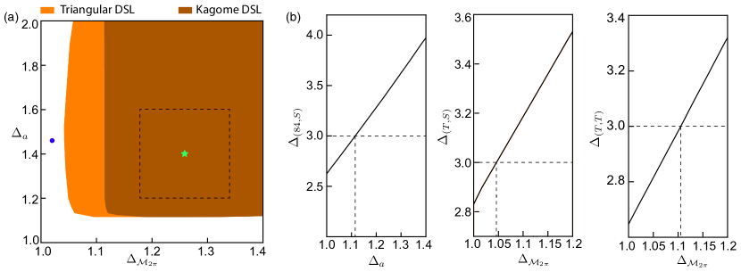
We now turn to the numerical bounds for the DSL. Requiring in bootstrap that operators which are singlets of the UV symmetry be irrelevant can provide lower bounds for the scaling dimension of several operators. This type of study was initiated in Nakayama and Ohtsuki (2016). In the case of DSL, as summarized in Sec. II.1, in order to have the triangular DSL be a stable critical phase, we shall have and . For the kagome DSL to be stable, we have two more requirements, and . We thus impose these conditions in the mixed correlator (between the fermion bilinear and the monopole ) bootstrap calculations. In this setup we identify OPE coefficients , and there are no ratios of OPE coefficients to scan. Somewhat disappointingly, unlike the mixed correlator bootstrap for the Wilson-Fisher CFT Kos et al. (2016, 2015), here the mixed correlator bootstrap does not produce any sharp signature for the QED3. Instead, we just get numerical bounds for as shown in Fig. 2(a). For the triangular DSL and kagome DSL, the allowed regions are slightly different. The large- result (blue circle) lies outside these regions, meaning that the large- monopole scaling dimension is inconsistent with DSL being a stable phase on any lattice. While the result from the lattice Monte Carlo simulation (green star) is consistent with the DSL being stable on both lattices.
We find that numerical bounds from the mixed correlator bootstrap are almost identical to the bounds from the single correlators (Fig. 2(b)). For example, from the single correlator of the fermion bilinear () we have if we require . Similarly, from the single correlator of the monopole () we have and if we require and , respectively. Other requirements such as and do not produce any tighter bounds. We have also explored other mixed correlators, including two-operator mix— with and with , as well as three-operator mix between any three of , , , . Some of these mixed correlators could produce bounds tighter than the single correlators (under aggressive gap assumptions), but no sharp signature of the QED3 is found.
III Stiefel liquid
III.1 Overview
Stiefel liquids Zou et al. (2021) are recently proposed 3d CFTs described by 3d non-linear sigma models on the Stiefel manifold , supplemented with a level- Wess-Zumino-Witten (WZW) term,
| (12) |
Here is a matrix field, which lives on the Stiefel manifold . The proposal is that, there are three fixed points as one tunes the coupling constant : 1) an ordered (attractive) fixed point at , which corresponds to a spontaneous symmetry breaking fixed point with the groundstate manifold ; 2) a repulsive fixed point at , which corresponds to the order-disorder transition; 3) a disordered (attractive) fixed point at , which is conjectured to be conformal. This conjectured disordered conformal fixed point is the Stiefel liquid, and we label it as SLN,k. The global symmetry of SLN,k is for odd , and is for even . The most important operator of SL(N,k) is the order parameter field , which is the bi-vector of and .
The non-linear sigma model is non-renormalizable in 3d, making it hard to study analytically. Interestingly, SLN,k has a simple UV completion when . SL5,k is dual to a gauge theory with Dirac fermions coupled to a gauge field, and the order parameter field can be identified as the fermion bilinear operator that is a vector. SL6,k is dual to a gauge theory with Dirac fermions coupled to a gauge field, and the order parameter field can be identified as the lowest weight monopole operator that is a bi-vector of and . So SL6,1 is just the DSL we discussed in the previous section, and SL5,1 is the deconfined phase transition Senthil et al. (2004a, b); Nahum et al. (2015); Wang et al. (2017). There is no obvious gauge theory description for the SLN,k with , and SLN≥7,k is conjectured to be non-Lagrangian.
Based on the gauge theory description of SL5,k and SL6,k, we expect that for a given , the larger is, the more likely SLN,k will not be conformal. It will be interesting to determine the conformal window of SLN,k. A natural idea to bootstrap SLN,k is to bootstrap the order parameter field , which is the bi-vector of and . Below we will investigate the single correlator bootstrap of , and we will focus on . The OPE of is the same as that of the monopole in DSL,
| (13) | ||||
Again we are using the notation to denote the representation of the global symmetry of , with referring to the singlet, rank-2 anti-symmetric tensor, and rank-2 symmetric traceless tensor.
III.2 Numerical results

Similar to the monopole bootstrap discussed in the previous section, the numerical bound of has a kink. Moreover, this kink also seems to have an enhanced symmetry, namely . So this kink is the non-Wilson-Fisher kink Ohtsuki (2016); Li (2018); Li and Poland (2021); He et al. (2021a), and it should not be identified as the Stiefel liquid. We also bound other operators, but we do not find any interesting feature that can be related to the Stiefel liquid. Nevertheless, one piece of useful information that can be extracted is the lower bound of the scaling dimension of the order parameter field.
Possible realizations of SL7,1 have been proposed for the triangular and kagome quantum magnets Zou et al. (2021). For the proposed SL7,1 on the triangular lattice, we shall have . As shown in Fig. 3(a), this requires that . For the proposed realization on the kagome lattice, we shall have both and , requiring that as shown in Fig. 3(b). These bounds can also apply to SL7,k with .
IV Summary and Discussion
We used the conformal bootstrap to study the DSL and Stiefel liquid. For the DSL, i.e. QED3, we studied the single correlators of monopole (, bi-vector) and fermion bilinear ( adjoint), as well as their mixed correlators. We first discuss the kinks of numerical bounds of the lowest lying singlet. We provide clear evidence that these kinks should not be identified as the QED3 theory. We show that these kinks are likely to have enhanced symmetries, hence are the previously studied and non-Wilson-Fisher kinks. By requiring the critical phase to be stable on the triangular and the kagome lattice, we obtain rigorous numerical bounds for the scaling dimensions of certain operators of the Dirac spin liquid and the Stiefel liquid.
The scaling dimension of the fermion bilinear operator should be larger than . Furthermore, for the triangular magnets, the scaling dimension of the monopole operator should be larger ; while for the kagome magnets, the scaling dimension of the monopole operator should be larger . These bounds are consistent with the latest Monte Carlo simulation of the QED3. These rigorous bounds also apply to the DSL discussed in Ref. Calvera and Wang (2020).
We also bootstrapped the single correlator of the bi-vector, which applies to the Stiefel liquid with arbitrary . Similarly, we have obtained rigorous bounds assuming that the Stiefel liquid is a stable phase for several concrete proposed realizations.
The rigorous bounds obtained here might be useful to exclude future candidate theoretical models and materials for the DSL and Stiefel liquid. It will be exciting if the conformal bootstrap can provide more accurate information of these two critical theories. For the DSL, we have explored extensively the mixed correlators of various operators, including the fermion bilinear, monopole, monopole and a four-fermion operator. We did not find any sharp signature of the DSL in these mixed correlator studies. For example, as shown in the paper the mixed correlator of the fermion bilinear and monopole operator does not yield a tighter bound compared to the single correlator bound. Results of other operators mix are similar and are not illuminating to discuss in detail. It is worth remarking that there was an expectation that the monopole could be used to distinguish QED3 from its cousin QCD3 theories. This expectation, however, is incorrect, because the QCD3 theories with gauge fields also have monopole operators that share qualitatively similar properties (i.e. quantum numbers and scaling dimensions) Dyer et al. (2013) with the monopoles of QED3. Possible progress of bootstrapping QED3 might be made by using the idea of decoupling operators proposed by us in Ref. He et al. (2021b), which will be pursued in future.
Acknowledgements.
We would like to thank Chong Wang for discussions and Nikhil Karthik for communicating Monte Carlo results of the QED3. Research at Perimeter Institute is supported in part by the Government of Canada through the Department of Innovation, Science and Industry Canada and by the Province of Ontario through the Ministry of Colleges and Universities. This project has received funding from the European Research Council (ERC) under the European Union’s Horizon 2020 research and innovation programme (grant agreement no. 758903). The work of J.R. is supported by the DFG through the Emmy Noether research group “The Conformal Bootstrap Program” project number 400570283. The numerics is solved using SDPB program Simmons-Duffin (2015) and simpleboot (https://gitlab.com/bootstrapcollaboration/simpleboot). The computations in this paper were run on the Symmetry cluster of Perimeter institute.References
- Wen (2017) Xiao-Gang Wen, “Colloquium: Zoo of quantum-topological phases of matter,” Reviews of Modern Physics 89, 041004 (2017), arXiv:1610.03911 [cond-mat.str-el] .
- Rychkov and Vichi (2009) Vyacheslav S. Rychkov and Alessandro Vichi, “Universal Constraints on Conformal Operator Dimensions,” Phys. Rev. D 80, 045006 (2009), arXiv:0905.2211 [hep-th] .
- El-Showk et al. (2012) Sheer El-Showk, Miguel F. Paulos, David Poland, Slava Rychkov, David Simmons-Duffin, and Alessandro Vichi, “Solving the 3D Ising Model with the Conformal Bootstrap,” Phys. Rev. D 86, 025022 (2012), arXiv:1203.6064 [hep-th] .
- Kos et al. (2014a) Filip Kos, David Poland, and David Simmons-Duffin, “Bootstrapping the vector models,” JHEP 06, 091 (2014a), arXiv:1307.6856 [hep-th] .
- Kos et al. (2014b) Filip Kos, David Poland, and David Simmons-Duffin, “Bootstrapping Mixed Correlators in the 3D Ising Model,” JHEP 11, 109 (2014b), arXiv:1406.4858 [hep-th] .
- El-Showk et al. (2014) Sheer El-Showk, Miguel F. Paulos, David Poland, Slava Rychkov, David Simmons-Duffin, and Alessandro Vichi, “Solving the 3d Ising Model with the Conformal Bootstrap II. c-Minimization and Precise Critical Exponents,” J. Stat. Phys. 157, 869 (2014), arXiv:1403.4545 [hep-th] .
- Kos et al. (2015) Filip Kos, David Poland, David Simmons-Duffin, and Alessandro Vichi, “Bootstrapping the O(N) Archipelago,” JHEP 11, 106 (2015), arXiv:1504.07997 [hep-th] .
- Kos et al. (2016) Filip Kos, David Poland, David Simmons-Duffin, and Alessandro Vichi, “Precision Islands in the Ising and Models,” JHEP 08, 036 (2016), arXiv:1603.04436 [hep-th] .
- Simmons-Duffin (2017) David Simmons-Duffin, “The Lightcone Bootstrap and the Spectrum of the 3d Ising CFT,” JHEP 03, 086 (2017), arXiv:1612.08471 [hep-th] .
- Rong and Su (2018a) Junchen Rong and Ning Su, “Bootstrapping minimal superconformal field theory in three dimensions,” (2018a), arXiv:1807.04434 [hep-th] .
- Atanasov et al. (2018) Alexander Atanasov, Aaron Hillman, and David Poland, “Bootstrapping the Minimal 3D SCFT,” JHEP 11, 140 (2018), arXiv:1807.05702 [hep-th] .
- Iliesiu et al. (2016) Luca Iliesiu, Filip Kos, David Poland, Silviu S. Pufu, David Simmons-Duffin, and Ran Yacoby, “Bootstrapping 3D fermions,” Journal of High Energy Physics 2016, 120 (2016), arXiv:1508.00012 [hep-th] .
- Iliesiu et al. (2018) Luca Iliesiu, Filip Kos, David Poland, Silviu S. Pufu, and David Simmons-Duffin, “Bootstrapping 3D fermions with global symmetries,” Journal of High Energy Physics 2018, 36 (2018), arXiv:1705.03484 [hep-th] .
- Chester et al. (2019) Shai M. Chester, Walter Landry, Junyu Liu, David Poland, David Simmons-Duffin, Ning Su, and Alessandro Vichi, “Carving out OPE space and precise model critical exponents,” (2019), arXiv:1912.03324 [hep-th] .
- Chester et al. (2020) Shai M. Chester, Walter Landry, Junyu Liu, David Poland, David Simmons-Duffin, Ning Su, and Alessandro Vichi, “Bootstrapping Heisenberg Magnets and their Cubic Instability,” arXiv e-prints , arXiv:2011.14647 (2020), arXiv:2011.14647 [hep-th] .
- Poland et al. (2019) David Poland, Slava Rychkov, and Alessandro Vichi, “The conformal bootstrap: Theory, numerical techniques, and applications,” Reviews of Modern Physics 91, 015002 (2019), arXiv:1805.04405 [hep-th] .
- Affleck and Marston (1988) Ian Affleck and J. Brad Marston, “Large-n limit of the heisenberg-hubbard model: Implications for high- superconductors,” Phys. Rev. B 37, 3774–3777 (1988).
- Wen and Lee (1996) Xiao-Gang Wen and Patrick A. Lee, “Theory of Underdoped Cuprates,” Phys. Rev. Lett. 76, 503–506 (1996), arXiv:cond-mat/9506065 [cond-mat] .
- Hastings (2000) M. B. Hastings, “Dirac structure, rvb, and goldstone modes in the kagomé antiferromagnet,” Phys. Rev. B 63, 014413 (2000).
- Hermele et al. (2005) Michael Hermele, T. Senthil, and Matthew P. A. Fisher, “Algebraic spin liquid as the mother of many competing orders,” Phys. Rev. B 72, 104404 (2005), arXiv:cond-mat/0502215 [cond-mat.str-el] .
- Hermele et al. (2008) Michael Hermele, Ying Ran, Patrick A. Lee, and Xiao-Gang Wen, “Properties of an algebraic spin liquid on the kagome lattice,” Phys. Rev. B 77, 224413 (2008), arXiv:0803.1150 [cond-mat.str-el] .
- Song et al. (2020) Xue-Yang Song, Yin-Chen He, Ashvin Vishwanath, and Chong Wang, “From spinon band topology to the symmetry quantum numbers of monopoles in dirac spin liquids,” Phys. Rev. X 10, 011033 (2020).
- Song et al. (2019) Xue-Yang Song, Chong Wang, Ashvin Vishwanath, and Yin-Chen He, “Unifying description of competing orders in two-dimensional quantum magnets,” Nature Communications 10, 4254 (2019), arXiv:1811.11186 [cond-mat.str-el] .
- Ran et al. (2007) Ying Ran, Michael Hermele, Patrick A Lee, and Xiao-Gang Wen, “Projected-wave-function study of the spin-1/2 heisenberg model on the kagomé lattice,” Physical review letters 98, 117205 (2007).
- Iqbal et al. (2013) Yasir Iqbal, Federico Becca, Sandro Sorella, and Didier Poilblanc, “Gapless spin-liquid phase in the kagome spin- heisenberg antiferromagnet,” Phys. Rev. B 87, 060405 (2013).
- Iqbal et al. (2016) Y. Iqbal, W.-J. Hu, R. Thomale, D. Poilblanc, and F. Becca, “Spin liquid nature in the Heisenberg J1-J2 triangular antiferromagnet,” Phys. Rev. B 93, 144411 (2016), arXiv:1601.06018 [cond-mat.str-el] .
- He et al. (2017) Yin-Chen He, Michael P. Zaletel, Masaki Oshikawa, and Frank Pollmann, “Signatures of dirac cones in a dmrg study of the kagome heisenberg model,” Phys. Rev. X 7, 031020 (2017).
- Hu et al. (2019) Shijie Hu, W. Zhu, Sebastian Eggert, and Yin-Chen He, “Dirac Spin Liquid on the Spin-1 /2 Triangular Heisenberg Antiferromagnet,” Phys. Rev. Lett. 123, 207203 (2019), arXiv:1905.09837 [cond-mat.str-el] .
- Karthik and Narayanan (2016a) Nikhil Karthik and Rajamani Narayanan, “No evidence for bilinear condensate in parity-invariant three-dimensional QED with massless fermions,” Phys. Rev. D 93, 045020 (2016a), arXiv:1512.02993 [hep-lat] .
- Karthik and Narayanan (2016b) Nikhil Karthik and Rajamani Narayanan, “Scale invariance of parity-invariant three-dimensional QED,” Phys. Rev. D 94, 065026 (2016b), arXiv:1606.04109 [hep-th] .
- Karthik and Narayanan (2019) Nikhil Karthik and Rajamani Narayanan, “Numerical determination of monopole scaling dimension in parity-invariant three-dimensional noncompact QED,” Phys. Rev. D 100, 054514 (2019), arXiv:1908.05500 [hep-lat] .
- Wang et al. (2017) Chong Wang, Adam Nahum, Max A Metlitski, Cenke Xu, and T Senthil, “Deconfined quantum critical points: symmetries and dualities,” Physical Review X 7, 031051 (2017).
- Gorbenko et al. (2018a) Victor Gorbenko, Slava Rychkov, and Bernardo Zan, “Walking, weak first-order transitions, and complex CFTs,” Journal of High Energy Physics 2018, 108 (2018a), arXiv:1807.11512 [hep-th] .
- Gorbenko et al. (2018b) Victor Gorbenko, Slava Rychkov, and Bernardo Zan, “Walking, Weak first-order transitions, and Complex CFTs II. Two-dimensional Potts model at ,” SciPost Physics 5, 050 (2018b), arXiv:1808.04380 [hep-th] .
- Kaveh and Herbut (2005) Kamran Kaveh and Igor F. Herbut, “Chiral symmetry breaking in three-dimensional quantum electrodynamics in the presence of irrelevant interactions: A renormalization group study,” Phys. Rev. B 71, 184519 (2005), arXiv:cond-mat/0411594 [cond-mat.supr-con] .
- Braun et al. (2014) Jens Braun, Holger Gies, Lukas Janssen, and Dietrich Roscher, “Phase structure of many-flavor QED3,” Phys. Rev. D 90, 036002 (2014), arXiv:1404.1362 [hep-ph] .
- Herbut (2016) Igor F. Herbut, “Chiral symmetry breaking in three-dimensional quantum electrodynamics as fixed point annihilation,” Phys. Rev. D 94, 025036 (2016), arXiv:1605.09482 [hep-th] .
- Di Pietro et al. (2016) Lorenzo Di Pietro, Zohar Komargodski, Itamar Shamir, and Emmanuel Stamou, “Quantum Electrodynamics in d =3 from the Expansion,” Phys. Rev. Lett. 116, 131601 (2016), arXiv:1508.06278 [hep-th] .
- Giombi et al. (2015) Simone Giombi, Igor R. Klebanov, and Grigory Tarnopolsky, “Conformal QEDd, -Theorem and the Expansion,” arXiv e-prints , arXiv:1508.06354 (2015), arXiv:1508.06354 [hep-th] .
- Jian et al. (2018) Chao-Ming Jian, Alex Thomson, Alex Rasmussen, Zhen Bi, and Cenke Xu, “Deconfined quantum critical point on the triangular lattice,” Phys. Rev. B 97, 195115 (2018), arXiv:1710.04668 [cond-mat.str-el] .
- García-Etxebarria and Regalado (2016) Iñaki García-Etxebarria and Diego Regalado, “{N}=3 four dimensional field theories,” Journal of High Energy Physics 2016, 83 (2016), arXiv:1512.06434 [hep-th] .
- Beem et al. (2016) Christopher Beem, Madalena Lemos, Leonardo Rastelli, and Balt C. van Rees, “The (2, 0) superconformal bootstrap,” Phys. Rev. D 93, 025016 (2016), arXiv:1507.05637 [hep-th] .
- Gukov (2017) Sergei Gukov, “Trisecting non-Lagrangian theories,” Journal of High Energy Physics 2017, 178 (2017), arXiv:1707.01515 [hep-th] .
- Argyres and Douglas (1995) Philip C Argyres and Michael R Douglas, “New phenomena in su (3) supersymmetric gauge theory,” Nuclear Physics B 448, 93–126 (1995).
- Maruyoshi and Song (2017) Kazunobu Maruyoshi and Jaewon Song, “ deformations and RG flows of SCFTs,” JHEP 02, 075 (2017), arXiv:1607.04281 [hep-th] .
- Zou et al. (2021) Liujun Zou, Yin-Chen He, and Chong Wang, “Stiefel liquids: possible non-Lagrangian quantum criticality from intertwined orders,” arXiv e-prints , arXiv:2101.07805 (2021), arXiv:2101.07805 [cond-mat.str-el] .
- Senthil et al. (2004a) T. Senthil, Ashvin Vishwanath, Leon Balents, Subir Sachdev, and Matthew P. A. Fisher, “Deconfined quantum critical points,” Science 303, 1490 (2004a).
- Senthil et al. (2004b) T. Senthil, Leon Balents, Subir Sachdev, Ashvin Vishwanath, and Matthew P. A. Fisher, “Quantum criticality beyond the landau-ginzburg-wilson paradigm,” Phys. Rev. B 70, 144407 (2004b).
- Nahum et al. (2015) Adam Nahum, P. Serna, J.T. Chalker, M. Ortuno, and A.M. Somoza, “Emergent so(5) symmetry at the Néel to valence-bond-solid transition,” Physical Review Letters 115 (2015), 10.1103/physrevlett.115.267203.
- Nakayama (2018) Yu Nakayama, “Bootstrap experiments on higher dimensional cfts,” International Journal of Modern Physics A 33, 1850036 (2018).
- Chester and Pufu (2016a) Shai M. Chester and Silviu S. Pufu, “Towards bootstrapping qed3,” Journal of High Energy Physics 2016 (2016a), 10.1007/jhep08(2016)019.
- Li (2018) Zhijin Li, “Solving qed3 with conformal bootstrap,” (2018), arXiv:1812.09281 [hep-th] .
- Chester and Pufu (2016b) Shai M. Chester and Silviu S. Pufu, “Anomalous dimensions of scalar operators in qed3,” Journal of High Energy Physics 2016 (2016b), 10.1007/jhep08(2016)069.
- Dyer et al. (2013) Ethan Dyer, Márk Mezei, and Silviu S. Pufu, “Monopole Taxonomy in Three-Dimensional Conformal Field Theories,” arXiv e-prints , arXiv:1309.1160 (2013), arXiv:1309.1160 [hep-th] .
- Xu (2008) Cenke Xu, “Renormalization group studies on four-fermion interaction instabilities on algebraic spin liquids,” Phys. Rev. B 78, 054432 (2008), arXiv:0803.0794 [cond-mat.str-el] .
- Ohtsuki (2016) Tomoki Ohtsuki, Applied Conformal Bootstrap, Ph.D. thesis, University of Tokyo (2016).
- Rong and Su (2018b) Junchen Rong and Ning Su, “Scalar CFTs and Their Large N Limits,” JHEP 09, 103 (2018b), arXiv:1712.00985 [hep-th] .
- Stergiou (2019) Andreas Stergiou, “Bootstrapping MN and Tetragonal CFTs in Three Dimensions,” SciPost Phys. 7, 010 (2019), arXiv:1904.00017 [hep-th] .
- Paulos and Zan (2019) Miguel F. Paulos and Bernardo Zan, “A functional approach to the numerical conformal bootstrap,” (2019), arXiv:1904.03193 [hep-th] .
- He et al. (2021a) Yin-Chen He, Junchen Rong, and Ning Su, “Non-Wilson-Fisher kinks of O(N) numerical bootstrap: from the deconfined phase transition to a putative new family of CFTs,” SciPost Physics 10, 115 (2021a), arXiv:2005.04250 [hep-th] .
- Li and Poland (2021) Zhijin Li and David Poland, “Searching for gauge theories with the conformal bootstrap,” Journal of High Energy Physics 2021, 172 (2021), arXiv:2005.01721 [hep-th] .
- Reehorst et al. (2020) Marten Reehorst, Maria Refinetti, and Alessandro Vichi, “Bootstrapping traceless symmetric scalars,” arXiv e-prints , arXiv:2012.08533 (2020), arXiv:2012.08533 [hep-th] .
- He et al. (2021b) Yin-Chen He, Junchen Rong, and Ning Su, “A roadmap for bootstrapping critical gauge theories: decoupling operators of conformal field theories in dimensions,” arXiv e-prints , arXiv:2101.07262 (2021b), arXiv:2101.07262 [hep-th] .
- Manenti and Vichi (2021) Andrea Manenti and Alessandro Vichi, “Exploring adjoint correlators in ,” arXiv e-prints , arXiv:2101.07318 (2021), arXiv:2101.07318 [hep-th] .
- Poland et al. (2012) David Poland, David Simmons-Duffin, and Alessandro Vichi, “Carving Out the Space of 4D CFTs,” JHEP 05, 110 (2012), arXiv:1109.5176 [hep-th] .
- Nakayama and Ohtsuki (2016) Yu Nakayama and Tomoki Ohtsuki, “Conformal Bootstrap Dashing Hopes of Emergent Symmetry,” Phys. Rev. Lett. 117, 131601 (2016), arXiv:1602.07295 [cond-mat.str-el] .
- Calvera and Wang (2020) Vladimir Calvera and Chong Wang, “Theory of Dirac spin liquids on spin- triangular lattice: possible application to -CrOOH(D),” arXiv e-prints , arXiv:2012.09809 (2020), arXiv:2012.09809 [cond-mat.str-el] .
- Simmons-Duffin (2015) David Simmons-Duffin, “A Semidefinite Program Solver for the Conformal Bootstrap,” JHEP 06, 174 (2015), arXiv:1502.02033 [hep-th] .