Follow-up of non-transiting planets detected by Kepler

Abstract

Context. The direct detection of new extrasolar planets from high-precision photometry data is commonly based on the observation of the transit signal of the planet as it passes in front of its star. Close-in planets, however, leave additional imprints in the light curve even if they do not transit. These are the so-called phase curve variations that include ellipsoidal, reflection and beaming effects.

Aims. In Millholland & Laughlin (2017), the authors scrutinized the Kepler database looking for these phase variations from non-transiting planets. They found 60 candidates whose signals were compatible with planetary companions. In this paper, we perform a ground-based follow-up of a sub-sample of these systems with the aim of confirming and characterizing these planets and thus validating the detection technique.

Methods. We used the CAFE and HERMES instruments to monitor the radial velocity of ten non-transiting planet candidates along their orbits. We additionally used AstraLux to obtain high-resolution images of some of these candidates to discard blended binaries that contaminate the Kepler light curves by mimicking planetary signals.

Results. Among the ten systems, we confirm three new hot-Jupiters (KIC 8121913 b, KIC 10068024 b, and KIC 5479689 b) with masses in the range 0.5-2 M_Jup and set mass constraints within the planetary regime for the other three candidates (KIC 8026887 b, KIC 5878307 b, and KIC 11362225 b), thus strongly suggestive of their planetary nature.

Conclusions. For the first time, we validate the technique of detecting non-transiting planets via their phase curve variations. We present the new planetary systems and their properties. We find good agreement between the RV-derived masses and the photometric masses in all cases except KIC 8121913 b, which shows a significantly lower mass derived from the ellipsoidal modulations than from beaming and radial velocity data.

1 Introduction

In the era of high-precision photometric space-based missions, the detection of extrasolar planets through the transit technique has been very fruitful. So far, more than 4300 planets have been found around other stars, with around three fourths of them detected by this technique. Since the launch of the CoRoT mission (Auvergne et al., 2009), the subsequent NASA planet hunter Kepler (Borucki et al., 2010) and its extended K2 mission (Howell et al., 2014) as well as its successor TESS (Ricker et al., 2014) have scrutinized the sky looking for these planetary fingerprints in the light curves of stellar sources. According to the NASA Exoplanet archive, more than 2400 planets were discovered with Kepler, more than 400 with K2, and presently 137 have been detected and confirmed by TESS using the transit method (Akeson et al., 2013).

Several years after the end of the prime Kepler mission, the high-quality data provided by this telescope are still being profitably mined. Although Kepler was tasked to find Earth-size planets around Solar-like stars, it explored an unexpectedly large range of planetary and orbital properties, including the first circumbinary planets, super-Earths, planets in highly eccentric orbits, and planets around giant stars, etc. (e.g., Doyle et al. 2011; Borucki et al. 2012; Ciceri et al. 2015; Lillo-Box et al. 2014, respectively).

The transit technique, however, does not by itself provide a full confirmation of the planet candidate signal, as other non-planetary configurations can mimic the imprint of a symmetric dip in the light curve (e.g., background eclipsing binaries, grazing binary eclipses, etc.). Also, any blended source residing inside the photometer aperture can contaminate the light curve and provide inaccurate estimates of the planet candidate’s parameters. Hence, additional follow-up is necessary from the ground. In practice, the confirmation of transiting planet candidates stems primarily from radial velocity (RV) follow-up, which can provide the mass of the transiting body and thus confirm its planetary nature.

The extraordinary quality of the Kepler photometry motivated the proposal of an alternate technique to detect and fully characterize (i.e., measure the mass and orbital configuration of) new planets. Previously used in binary systems, the detection of periodic modulations coupled with the orbital phase of the planet arose as a new potential detection technique (e.g., Faigler & Mazeh 2011). These photometric variations are mainly due to three effects: reflected stellar light, ellipsoidal modulations, and Doppler beaming (hereafter the REB modulations, see Fig. 1). The reflection effect depends directly on the planet-to-star separation, size, and the geometric albedo of the planet. The ellipsoidal variations are known to be caused by tidal effects produced by a close-in object (e.g., a planet) on the external layers of the star (Morris 1985). Since the amplitude of this modulation depends on the mass of the planet, it can potentially be used to both detect, confirm, and characterize planets. Finally, the Doppler beaming effect represents the photometric signature of the RV variations of the star induced by the planet motion when photometry is obtained on a fixed wavelength range (Hills & Dale, 1974; Rybicki & Lightman, 1979). The induced RV implies that the stellar spectrum is periodically blue-shifted and red-shifted. As a consequence, more or less light enters in the wavelength domain of the photometric filter, yielding sinusoidal flux variations with an amplitude that depends on the mass of the planet.

The REB modulations have already been used to detect and characterize close-in transiting planets from the Kepler sample (e.g., Mazeh et al. 2012; Lillo-Box et al. 2014). These systematic searches have established several interesting findings, including generally low (but occasionally quite large) hot Jupiter albedos (Demory & Seager, 2011) and repeated detections of shifts in the maximum of the phase curve away from the sub-stellar point. Though it is substantial, the sample size ($\sim$ 15) of Kepler transiting planets with detectable photometric variations (less than 5 with RV confirmations) is short of the count necessary to adequately understand the atmospheric properties in a population sense. It is therefore worthwhile to increase the number of planets with well-characterized optical phase curves by expanding the search to non-transiting planets. Moreover, the masses derived from these modulations seem to not fully match the measurements from RVs in the few (less than 5) cases where both techniques could be applied. This is theoretically attributed to the presence of hot stream clouds in the atmosphere of the hot-Jupiters causing a phase shift in the light curve modulations.

Millholland & Laughlin (2017) used a supervised machine learning approach to perform a systematic search of these modulations in the whole sample of 142 630 FGK Kepler stars without confirmed planets or KOIs (Kepler Objects of Interest). They identified 60 high-probability ($>$98%) non-transiting hot Jupiter candidates that could readily be confirmed with RVs (see Fig. 1). In this paper, we present the ground-based follow-up of the brightest sub-sample of these candidates. In Sect. 2, we present the targets and the observations. In Sect. 3, we perform a joint analysis of the light curve and RV data to confirm the planetary nature of some of the candidates and constrain the masses of the remaining sub-sample. In Sect. 4, we discuss the results of the analysis, and we conclude in Sect. 5.

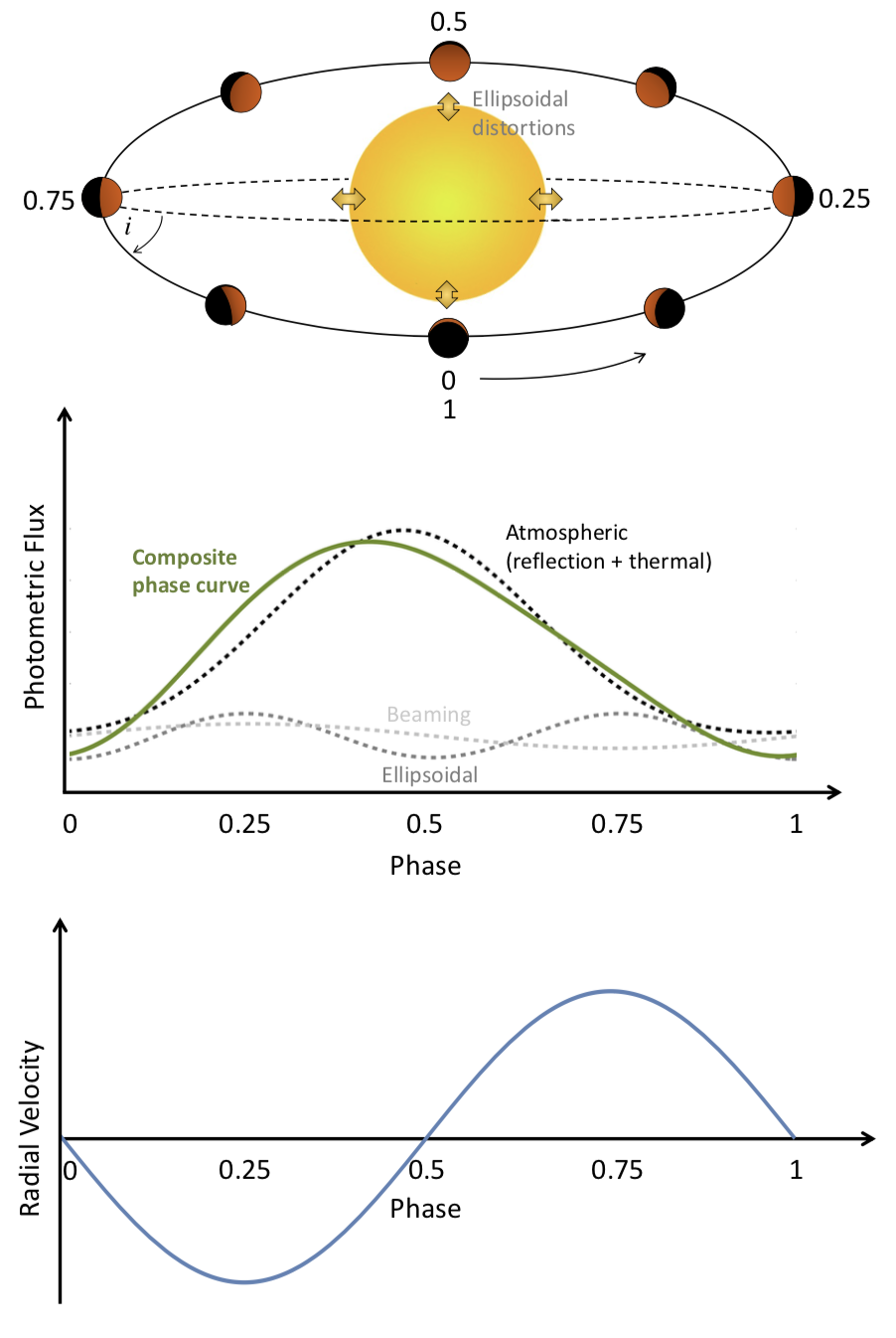
Figure 1: Schematic representation of the reflection, ellipsoidal and beaming (REB) modulations. Top panel shows the orbital path of the planet at different phases and two orbital inclinations. Middle panel shows the corresponding shape of the REB effects (dotted labelled lines) and the composite phase curve (green solid line). The bottom panel shows the corresponding RV signal with its appropriate phase relationship.

2 Follow-up observations

2.1 Target selection

This work is based on the follow-up of the Kepler non-transiting planet candidates detected by Millholland & Laughlin (2017) through the phase variations technique. Among the 60 candidates, we focused on those feasible with the Calar Alto Fiber-fed Echelle spectrograph (CAFE, Aceituno et al. 2013; Lillo-Box et al. 2020). We selected ten of the brightest candidates (Kp $<14$ mag) displaying photometric periods of a few days ($P<5$ days) and with estimated RV amplitudes ($K\sin{i}$) from the photometric phase curve analysis feasible with CAFE ($K\sin{i}>10$ m/s). Table 1 lists our initial selection of targets.

Table 1: List of targets selected for initial follow-up. The columns are the Kepler Input Catalog (KIC) target ID, the Kepler magnitude $K_{p}$ (Mathur et al., 2017), and the estimated orbital period $P$ and $K\sin{i}$ of the candidate non-transiting hot Jupiter determined from Millholland & Laughlin (2017) (where $K$ is the radial velocity semi-amplitude and $i$ is the unknown orbital inclination), and whether they were observed in high-resolution imaging (HRI). The last four targets correspond to those with large rotation velocities preventing precise radial velocity extraction.

KIC	$K_{p}$	$P$ (days)	$K\sin{i}$ (m/s)	HRI
8121913	11.7	$3.2943\pm 0.0003$	$61\pm 66$	Yes
11362225	12.0	$2.7513\pm 0.0021$	$103\pm 71$	Yes
10068024	13.1	$2.0735\pm 0.0012$	$229\pm 243$	Yes
5878307	13.6	$2.0466\pm 0.0013$	$116\pm 112$	Yes
5479689	13.8	$1.7012\pm 0.0008$	$158\pm 111$	Yes
8026887	13.9	$1.9232\pm 0.0009$	$234\pm 113$	Yes
6783562	13.6	$2.0883\pm 0.0014$	$243\pm 267$	No
5001685	14.0	$2.2906\pm 0.0014$	$221\pm 108$	No
8042004	13.3	$1.9498\pm 0.0011$	$42\pm 39$	No
10931452	12.7	$2.7001\pm 0.0023$	$108\pm 91$	Yes

2.2 Kepler light curves

In Section 3.2, we will perform a joint fit of the RV and light curve data. For the Kepler light curves, we use the same pre-processing techniques as Millholland & Laughlin (2017); further details can be found therein. We began with the pre-search data conditioning (PDC) photometry (Smith et al., 2012; Stumpe et al., 2012, 2014) provided by the Kepler Science Center. We performed two types of detrending: (1) an initial sliding polynomial fit, which was first used to identify candidate periodic signals using a Lomb-Scargle periodogram, and (2) a two-component detrending on the candidate signals, which simultaneously fit a sinusoidal phase curve component and a sliding polynomial stellar variability component. Using this latter fit, we created the detrended light curve by dividing the PDC light curve by the polynomial component of the fit. These detrended light curves will be used in Section 3.2, where we will phase fold and bin the light curve data for our joint fit.

2.3 Astralux high-spatial resolution imaging

We used the AstraLux instrument (Hormuth et al., 2008) at the 2.2m telescope in Calar Alto observatory to obtain high-spatial resolution images of seven of the selected candidates. AstraLux is a simple fast-readout camera that performs the so-called lucky imaging technique on a 24x24 arcsec maximum field-of-view (FOV), with the possibility of windowing to smaller FOVs in order to gain in readout time and thus reduce the exposure time. The instrument has demonstrated an excellent performance and has already shown a key contribution to the Kepler Follow-up Observing program (KFOP) in Lillo-Box et al. (2012, 2014); Furlan et al. (2017) and in key results from the K2 (e.g., Santerne et al. 2018; Barros et al. 2017) and TESS (e.g., Armstrong et al. 2020; Bluhm et al. 2020; Soto et al. 2021) missions.

Seven of the targets were observed with AstraLux on 13 August 2019 under 1.2 arcsec mean seeing conditions and good transparency conditions. One of the images (corresponding to KIC 8026887) is too noisy to be useful given a sudden worsening of the weather conditions. Hence, we here analyze the remaining images for six of our targets. The datacubes were reduced with the automatic pipeline running at the observatory (Hormuth et al., 2008). This pipeline performs the basic reduction of the data and then selects the 10% best frames (according to their Strehl ratio, Strehl 1902) and aligns and stack the frames to get the final high-spatial resolution image. These images are subsequently analyzed by our pipeline to detect possible blended sources and to obtain the contrast curves and estimate the maximum contamination in the Kepler light curves (see Lillo-Box et al. 2012, 2014 for details on how these contrast curves are estimated). The resulting contrast curves and AstraLux images are presented in Fig. 2.

The high-resolution images do not show any signs of close companions within 3 arcsec for any of the observed targets. Additionally, the contrast curves discard photometric contamination from undetected companions below 1%. This is sufficient to ensure that the source of the photometric phase variations detected in Millholland & Laughlin (2017) is the bright (and only) target in the field of view. Given this result, we will assume throughout our analysis that the only source in the Kepler aperture and hence the only contributor to the photometric signal is the target star.

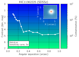
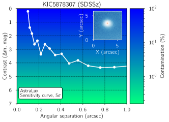
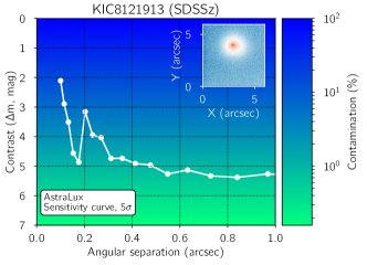
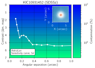
Figure 2: Results of the analysis of the high-spatial resolution images obtained with the AstraLux lucky-imaging instrument. Each panel shows the contrast curve calculated as in Lillo-Box et al. (2014) as a white line. The color-code of the contrast curve represents the contamination produced by a blended star of the given magnitude contrast as shown in the color bar. The inset panel displays the AstraLux image, with redder colors indicating more intensity.

2.4 CAFE high-resolution spectra

We used the CAFE instrument (Aceituno et al., 2013) with its recently upgraded capabilities (Lillo-Box et al., 2020) to perform a systematic RV follow-up of the selected planet candidates. CAFE is a fiber-fed high-resolution (R$=63\,000$) echelle spectrograph located in the coudé room of the 2.2m telescope at the Calar Alto observatory (Almería, Spain). Although the instrument has been operating since 2012, in 2016 its grating suffered a strong degradation that affected its efficiency and necessitated its retirement. This was taken as an opportunity to perform additional upgrades alongside the exchange of the grating. These improvements included a new double scrambler, introduction of temperature control of the isolated room where the instrument is located, and development of a new Python-based public pipeline (CAFExtractor, see Lillo-Box et al. 2020) that automatically reduces the data and provides high-level data-products like precise RV measurements using the cross-correlation technique (Baranne et al., 1996). These new capabilities were commissioned during 2018 and 2019, and the instrument was brought to full operation in April 2019. We refer the interested reader to Lillo-Box et al. (2020) for additional details on the new capabilities of CAFE.

The observations were carried out in May-August 2019 under the approved program ID H19-2.2-007 (PI: Lillo-Box). In total, we obtained 53 spectra from the ten targets. We used the new CAFExtractor pipeline to reduce the spectra and obtain the RVs. The pipeline includes an option to fit the CCF by using either a Gaussian profile (by default) or a rotational profile for the rapidly rotating stars (recommended for stars with v$\sin{i}>10$ km/s). The rotational profile is defined as in Gray (2005) and it has already been used in several programs that obtained precise RV measurements of rapidly rotating stars (e.g., Santerne et al. 2012; Aller et al. 2018). For cases with v$\sin{i}>10$ km/s, we used this approach, while for v$\sin{i}<10$ km/s, we used the usual Gaussian profile. In four out of the ten observed targets, either the CCF was too broad to extract meaningful RVs (KIC 6783562 and KIC 10931452) or the phase coverage was insufficient to perform a relevant analysis (KIC 5001685 and KIC 8042004). Hence, these targets are not further addressed in this paper. The extracted RVs and the properties of the CCF for the remaining six targets are shown in Tables 4 to 9.

2.5 HERMES/Mercator high-resolution spectra

We observed five of the targets from the selected sample with the high-resolution fiber-fed HERMES spectrograph (Raskin et al., 2011) at the Mercator telescope in La Palma in August 2020. HERMES is a sibling of the CORALIE instrument at La Silla. It provides a resolution of R=85 000 and a wavelength coverage of 377-900 nm. We used the simultaneous wavelength calibration mode, which uses a second fiber to inject a Thorium-Argon spectrum in between the science orders to monitor the nightly drift of the wavelength calibration for precise RV measurements. The instrument’s automatic pipeline provides the basic reduction of the spectra. We measured the RVs by following a similar procedure as described for the CAFE spectra, with a new mask adapted for this wavelength coverage and resolution. The extracted RVs and the properties of the CCF are shown in Tables 4 to 9.

3 Analysis

3.1 Radial velocity standalone modeling

We first performed a RV analysis of the CAFE data, since the number of RV measurements from the HERMES instrument was low for this preliminary analysis. Given the limited number of observations for most of the systems, we used a simplistic RV model that assumes circular orbits (likely a good approximation given the short periods of these candidates) and adopts Gaussian priors on the period and time of conjunction obtained from the light curve analysis in Millholland & Laughlin (2017). Consequently, the only two free parameters of the model are the systemic velocity (V_sys) and the semi-amplitude of the RV signal ($K$). For each of these parameters, we assumed a uniform prior with broad ranges corresponding to $\mathcal{U}(-100,100)$ km/s for V_sys and $\mathcal{U}(0.0,10)$ km/s for $K$.

We used the Markov Chain Monte Carlo affine invariant ensemble sampler emcee (Goodman & Weare, 2010; Foreman-Mackey et al., 2013) to explore the posterior probability of the two parameters. We ran a first set of 20 walkers with 10 000 steps per walker to identify the maximum likelihood location of the parameter space. Then we ran another 10 walkers with 10 000 steps per walker in a nearby region around this maximum likelihood location of the parameter space to properly sample the posterior distributions. The results are shown in Figs. 3 and 4, and the priors, median and confidence levels of the posterior distributions for each parameter are shown in Tables 10 to 15.

Among the six systems with appropriate phase coverage, we find clear detection in three of the targets (KIC 8121913, KIC 10068024, and KIC 5479689), see Fig. 3. In these cases, the RV semi-amplitude is detected with a confidence larger than 99.7% (corresponding to $3\sigma$) and thus are considered as confirmed planets. In two other cases (KIC 5878307 and KIC 11362225, see Fig. 4), the data is insufficient to measure the planet mass but the low amplitude of the RV variations and the absence of contaminants in the AstraLux images validate their planetary nature. In the case of KIC 8026887, we find either a large amplitude of several hundred of meters per second or a strong linear trend with a smaller RV amplitude. Additionally, by using a period equal to twice the photometric period ($2\times P=3.8464$ days), we find a clear signal compatible with a Keplerian model with $K\sim 610\pm 180$ m/s (see Fig. 4, right panel). This is further investigated in the joint light curve and radial velocity analysis in the next section.

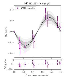
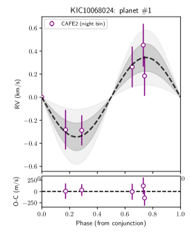
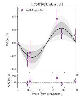
Figure 3: Phase-folded radial velocity curves for the three planets confirmed in this paper. The solid open symbols represent nightly binned values when more than one observation are available on a given night (although we note that the analysis in the paper has been done using the individual measurements). The median radial velocity model is represented by the black dashed line and the 67.8% and 95% confidence intervals are displayed as dark grey and light grey shaded regions around the median model.

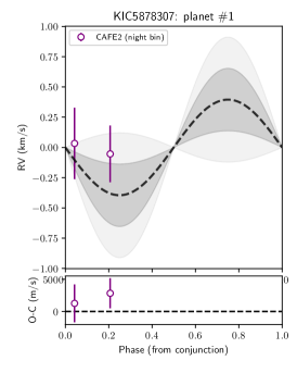
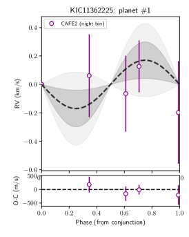
Figure 4: Phase-folded radial velocity curves for the two planets where only upper limits to the planet mass are possible (left and middle panels) and the case of KIC 8026887 with the period equal to twice the photometric period found in Millholland & Laughlin (2017). The solid open symbols represent nightly binned values when more than one observation are available on a given night (although we note that the analysis in the paper has been done using the individual measurements). The median radial velocity model is represented by the black dashed line and the 67.8% and 95% confidence intervals are displayed as dark grey and light grey shaded regions around the median model.

3.2 Joint radial velocity and light curve modeling

To examine the consistency of the RV observations and Kepler light curves, we performed a simultaneous fit of the two datasets for the four targets with sufficiently precise RVs: KIC 8121913, KIC 10068024, KIC 5479689, and KIC 8026887. The key goal of this simultaneous fit is to verify that the periods and phases suggested by the photometric detections are consistent with the RVs. Moreover, we also wish to investigate whether the companion mass estimates agree between the two datasets. Here we adopt a fitting approach that is as simplified as possible, on account of our relatively small number of RV data points and our goal to simply demonstrate RV and light curve consistency.

We model the phase curve variations using a four-component sum of sinusoids at the orbital phase

$$\phi\equiv(t-T_{0})/P,$$ (1)

where $T_{0}$ is the epoch of inferior conjunction (or the transit time if the companion is transiting):

$$\begin{split}F(\phi)&=A_{0}-A_{\mathrm{refl}}\cos(2\pi(\phi+\delta))\\ &-A_{\mathrm{ellip}}\cos(4\pi\phi)+A_{\mathrm{beam}}\sin(2\pi\phi).\end{split}$$ (2)

Here, $\delta$ is a phase offset in peak brigtness of the reflection component, and $A_{\mathrm{refl}}$, $A_{\mathrm{ellip}}$, and $A_{\mathrm{beam}}$ are positive quantities representing the photometric amplitudes of the atmospheric/reflection, ellipsoidal, and beaming components of the phase curve (Esteves et al., 2015; Shporer, 2017). These amplitudes will be treated as free parameters in our model. In Section 4.1, we will describe the origin of these phase curve components and their approximate relationships to fundamental physical and orbital parameters. We will also verify that they have been fit with reasonable values.

This four-component phase curve model is fit to the detrended Kepler light curves introduced in Section 2.2. These light curves are phase-folded using the period $P$ and epoch $T_{0}$ from equation 1 (both of which are free parameters in the fit) and binned into 400 bins, with the $j$th bin having mean flux, $F_{j}$, and standard deviation, $\sigma_{F,j}$.

We now proceed to the RV component of the joint fit. We model the Doppler velocities simply as

$$v(t)=-K\sin(2\pi\phi)+\dot{\gamma}(t-T_{0})+\gamma_{\mathrm{inst}},$$ (3)

where we have assumed a negligible orbital eccentricity. The RV semi-amplitude, $K$, is strictly positive, and $\phi$ and $T_{0}$ are the same phase and epoch as defined in equation 1. In addition to the sinusoidal signal, we include a long-term linear trend with acceleration $\dot{\gamma}$ and instrument-specific offset, $\gamma_{\mathrm{inst}}$.

We perform a joint RV and phase curve fit to the observations using the standard practices of Bayesian inference. The log-likelihood is here composed of the sum of the individual log-likelihoods of the RV and light curve datasets:

$$\ln\mathcal{L}=\ln\mathcal{L}_{\mathrm{RV}}+\ln\mathcal{L}_{\mathrm{LC}}.$$ (4)

Assuming Gaussian-distributed noise, the RV log-likelihood is

$$\ln\mathcal{L}_{\mathrm{RV}}=-\frac{1}{2}\sum_{j}\left[{\frac{(v_{j}-v_{\mathrm{mod}}(t_{j}))^{2}}{(\sigma_{v,j}^{2}+\sigma_{\mathrm{jit,inst}}^{2})}}+\ln(2\pi[\sigma_{v,j}^{2}+\sigma_{\mathrm{jit,inst}}^{2}])\right].$$ (5)

Here, $v_{j}$ and $\sigma_{v,j}$ are the $j$th velocity measurement and measurement error, and $v_{\mathrm{mod}}(t_{j})$ is the model RV (equation 3) at time $t_{j}$.

Similarly, the light curve log-likelihood is given by

$$\ln\mathcal{L}_{\mathrm{LC}}=-\frac{1}{2}\sum_{j}{\left[\frac{(F_{j}-F_{\mathrm{mod}}(\phi_{j}))^{2}}{\sigma_{F,j}^{2}}+\ln(2\pi\sigma_{F,j}^{2})\right]},$$ (6)

where $F_{j}$ and $\sigma_{F,j}$ are the $j$th measurement and error resulting from the folded and binned light curve data. $F_{\mathrm{mod}}(\phi_{j})$ is the model phase curve (equation 2) at phase $\phi_{j}$.

The posterior distributions of the parameters were sampled through the Markov Chain Monte Carlo affine invariant ensemble sampler emcee (Goodman & Weare, 2010; Foreman-Mackey et al., 2013) using uniform priors and the likelihood function given by equations 4 – 6. We collect 20,000 samples across 200 chains, discarding the first 5,000 samples as burn-in. Convergence was assessed by inspecting trace plots to see that the chains were well-mixed. We provide corner plots of the joint posterior parameter distributions in Appendix B.

The results of the joint fit are presented in Table LABEL:tab:_joint_fit, and the best-fitting models for KIC 8121913, KIC 10068024, and KIC 5479689 are displayed in Figure 5. We observe that consistent solutions for the joint RV/phase curve fit can be found for these systems. Specifically, there are sets of $P$ and $T_{0}$ for which the two datasets agree within uncertainties. The amplitudes of the phase curve and RV signals are also generally consistent in terms of the physical system parameters they correspond to, as we will discuss in Section 4.1.

In the case of KIC 8026887, the phase curve clearly shows ellipsoidal variations when folded at $P=1.9232$ days. Hence the double period hypothesis is unlikely. In any case, we tested it to ensure that the $P=1.9$ days is able to jointly model the RV and LC data. We then tested four models including priors on the period and turning on and off the linear trend. We then estimated the Bayesian evidence for the four models and concluded that the model with $P=1.9$ and the linear trend shows the largest evidence for the current dataset. This model is able to reconcile both RVs and light curve modulations and provides a planet mass of $3.44\pm 0.42$ M_jup. The difference in log-evidence is $+7$ compared to the model without a linear trend and $+135$ compared to the model with $2\times P$. The candidate absolute mass is hence significantly detected and we can hence validate the planetary nature of this candidate. Given the poor radial velocity phase coverage, however, we remain conservative and do not claim confirmation yet.

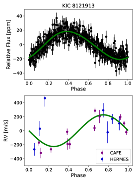
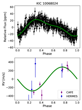
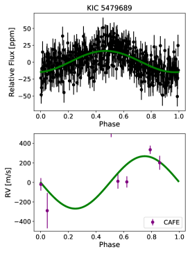
Figure 5: Results of the joint phase curve (upper panels) and radial velocity (lower panels) fits for KIC 8121913, KIC 10068024, and KIC 5479689 (see Sect. 3.2)

Table 2: Results of the joint fits to the radial velocity and light curve data.

	KIC 8121913	KIC 10068024	KIC 5479689
Orbital parameters
$T_{0}$ (BJD)	$2456427.84^{+0.04}_{-0.05}$	$2456424.23^{+0.05}_{-0.05}$	$2456423.76^{+0.09}_{-0.15}$
$P$ (days)	$3.294601^{+0.000013}_{-0.00022}$	$2.073549^{+0.000008}_{-0.000177}$	$1.701531^{+0.000008}_{-0.000419}$
Phase curve parameters
$A_{0}$ (ppm)	$-0.03^{+0.38}_{-0.38}$	$-0.08^{+0.52}_{-0.53}$	$-0.33^{+0.73}_{-0.81}$
$A_{\mathrm{refl}}$ (ppm)	$14.1^{+1.3}_{-1.1}$	$18.7^{+1.1}_{-1.0}$	$14.1^{+1.3}_{-1.5}$
$A_{\mathrm{ellip}}$ (ppm)	$2.2^{+0.5}_{-0.5}$	$5.8^{+0.8}_{-0.8}$	$0.3^{+0.5}_{-0.2}$
$A_{\mathrm{beam}}$ (ppm)	$11.8^{+2.8}_{-2.7}$	$9.7^{+4.2}_{-4.3}$	$2.5^{+2.4}_{-1.8}$
$\delta$	$0.01^{+0.03}_{-0.03}$	$-0.0^{+0.04}_{-0.04}$	$0.02^{+0.02}_{-0.02}$
RV parameters
$K$ (m/s)	$224.14^{+36.95}_{-38.85}$	$276.7^{+46.4}_{-47.13}$	$82.37^{+65.24}_{-24.51}$
$\gamma_{\mathrm{CAFE}}$ (m/s)	$2826.4^{+2471.1}_{-2435.1}$	$8582.9^{+4956.7}_{-4235.6}$	$26675.9^{+5116.7}_{-4930.2}$
$\gamma_{\mathrm{HERMES}}$ (m/s)	$3278.6^{+2929.4}_{-2877.1}$	$9982.8^{+5759.0}_{-4933.8}$	$34211.5^{+10575.7}_{-10289.3}$
$\dot{\gamma}$ (m/s/day)	$-1.28^{+1.1}_{-1.12}$	$-3.8^{+1.88}_{-2.2}$	$-11.79^{+2.19}_{-2.28}$
$\sigma_{\mathrm{jit},\mathrm{CAFE}}$ (m/s)	$82.54^{+11.77}_{-15.54}$	$60.66^{+27.23}_{-36.66}$	$93.17^{+5.01}_{-10.47}$
$\sigma_{\mathrm{jit},\mathrm{HERMES}}$ (m/s)	$94.21^{+4.32}_{-9.02}$	$48.89^{+35.09}_{-33.5}$	$51.12^{+33.35}_{-34.3}$
Derived parameters
$M_{p}\sin{i}$ from $K$ ($M_{\mathrm{Jup}}$)	$2.1^{+0.4}_{-0.4}$	$2.0^{+0.4}_{-0.4}$	$0.5^{+0.4}_{-0.1}$
$M_{p}\sin{i}$ from $A_{\mathrm{ellip}}$ ($M_{\mathrm{Jup}}$)	$0.3^{+0.2}_{-0.1}$	$0.8^{+2.1}_{-0.5}$	$0.1^{+0.2}_{-0.1}$
$M_{p}\sin{i}$ from $A_{\mathrm{beam}}$ ($M_{\mathrm{Jup}}$)	$2.3^{+0.6}_{-0.5}$	$1.5^{+0.6}_{-0.7}$	$0.3^{+0.3}_{-0.2}$
$\alpha_{\mathrm{ref}}{R_{p}}^{2}\sin{i}\ ({R_{\mathrm{Jup}}}^{2})$	$1.56^{+0.18}_{-0.15}$	$0.99^{+0.11}_{-0.11}$	$0.49^{+0.05}_{-0.05}$

4 Discussion

4.1 Consistency of RVs and phase curve component amplitudes

Table 3: Stellar parameters adopted for KIC 8121913, KIC 10068024, and KIC 5479689, taken from the Gaia-Kepler Stellar Properties Catalog (Berger et al., 2020).

	KIC 8121913	KIC 10068024	KIC 5479689
$M_{\star}\ (M_{\odot})$	$1.456^{+0.069}_{-0.15}$	$1.22^{+0.175}_{-0.139}$	$0.966^{+0.03}_{-0.04}$
$R_{\star}\ (R_{\odot})$	$2.233^{+0.054}_{-0.056}$	$1.574^{+0.525}_{-0.37}$	$0.894^{+0.017}_{-0.016}$
$T_{\mathrm{eff}}$ (K)	$5975.3^{+110.2}_{-109.4}$	$6118.4^{+127.2}_{-121.2}$	$5459.1^{+90.0}_{-85.2}$
Fe/H	$0.252^{+0.128}_{-0.17}$	$0.01^{+0.153}_{-0.174}$	$0.161^{+0.116}_{-0.115}$
$\log g$	$3.896^{+0.032}_{-0.05}$	$4.092^{+0.183}_{-0.195}$	$4.52^{+0.015}_{-0.024}$

In the previous section, we treated the phase curve component amplitudes as free parameters within the joint RV/phase curve fit. These amplitudes are not truly free parameters, however, since they stem from physical effects in the star-planet system. Thus, the comparison of the phase curve component amplitudes to one another and to the RV semi-amplitudes can inform whether the joint fits are physically consistent. Here we will describe the relation of the amplitudes to physical parameters and assess their consistency. Within this, we will adopt stellar parameters from the Gaia-Kepler Stellar Properties Catalog (Berger et al., 2020); these are provided in Table 3.

The atmospheric component of optical phase curves, $A_{\mathrm{refl}}$, includes both light from the primary star reflected off the companion, as well as thermal emission from the companion itself. It is generally difficult to separate reflected light from thermal emission, and it depends on the system as to which dominates. The amplitude of the atmospheric component is given by (Shporer, 2017),

$$\begin{split}A_{\mathrm{refl}}&\approx\frac{\alpha_{\mathrm{refl}}}{10}\left(\frac{R_{p}}{a}\right)^{2}\sin{i}\\ &\approx 57\alpha_{\mathrm{refl}}\sin{i}\left(\frac{M_{\star}}{M_{\odot}}\right)^{-2/3}\left(\frac{P}{\mathrm{day}}\right)^{-4/3}\left(\frac{R_{p}}{R_{\mathrm{J}}}\right)^{2}\mathrm{ppm}.\end{split}$$ (7)

Here $\alpha_{\mathrm{refl}}$ is an order-unity coefficient that depends on the planet’s albedo and the efficiency of heat redistribution.

In addition to phase modulations from the planet’s atmospheric brightness, there are also gravitationally-induced photometric signals from the host star. The phase component due to Doppler beaming (also known as Doppler boosting) stems from periodic blueshifts and redshifts of the stellar spectrum in response to the orbiting planet. The amplitude of the beaming component is given by

$$\begin{split}A_{\mathrm{beam}}&\approx\frac{4K\alpha_{\mathrm{beam}}}{c}\\ &\approx 2.7\alpha_{\mathrm{beam}}\left(\frac{P}{\mathrm{day}}\right)^{-1/3}\left(\frac{M_{\star}}{M_{\odot}}\right)^{-2/3}\left(\frac{M_{p}\sin{i}}{M_{\mathrm{J}}}\right)\mathrm{ppm}.\end{split}$$ (8)

Here, $K$ is the radial velocity semi-amplitude, $c$ is the speed of light and $\alpha_{\mathrm{beam}}$ is an order-unity coefficient equal to the photon-weighted bandpass-integrated beaming factor.

The second gravitational signal results from the ellipsoidal distortion of the host star due to tidal potential of the companion. This signal is dominated by a $\cos(4\pi\phi)$ term, although a more complete expansion includes smaller amplitude harmonics such as $\cos(2\pi\phi)$ and $\cos(6\pi\phi)$, which we have ignored in equation 2 for simplicity. The photometric amplitude of the ellipsoidal distortion is approximately

$$\begin{split}A_{\mathrm{ellip}}&\approx\frac{M_{p}\alpha_{\mathrm{ellip}}\sin^{2}{i}}{M_{\star}}\left(\frac{R_{\star}}{a}\right)^{3}\\ &\approx 13\alpha_{\mathrm{ellip}}\sin{i}\left(\frac{R_{\star}}{R_{\odot}}\right)^{3}\left(\frac{M_{\star}}{M_{\odot}}\right)^{-2}\left(\frac{P}{\mathrm{day}}\right)^{-2}\left(\frac{M_{p}\sin{i}}{M_{\mathrm{J}}}\right)\mathrm{ppm}.\end{split}$$ (9)

The $\alpha_{\mathrm{ellip}}$ coefficient is order-unity, and it relates to the stellar limb darkening and gravity darkening,

$$\alpha_{\mathrm{ellip}}=\frac{3(15+u)(1+g)}{20(3-u)},$$ (10)

where $u$ is the linear limb darkening coefficient and $g$ is the gravity darkening coefficient (Claret & Bloemen, 2011).

To investigate the consistency of the phase curve components and the RV semi-amplitudes for each system, we will compare their respective constraints on $M_{p}\sin{i}$. The minimum mass $M_{p}\sin{i}$ is most robustly constrained from the RV semi-amplitude $K$, but $A_{\mathrm{beam}}$ and $A_{\mathrm{ellip}}$ also provide weak estimates. We first solve equations 8 and 9 for $M_{p}\sin{i}$. Next, we use the posterior samples from the joint fits in Section 3.2 and the stellar parameter estimates (Table 3) to calculate the posterior distributions of $M_{p}\sin{i}$. Specifically, for the stellar parameters, we sample from distributions of $M_{\star}$ and $R_{\star}$ consistent with the observed means and error estimates in Table 3. The $A_{\mathrm{ellip}}$ amplitude includes an extra factor of $\sin{i}$ ($A_{\mathrm{ellip}}\propto M_{p}\sin^{2}{i}$; equation 9), so we average over it by assuming an isotropic distribution of the inclination. As for the order-unity coefficients $\alpha_{\mathrm{beam}}$ and $\alpha_{\mathrm{ellip}}$, we set them to fixed values based on simple linear relationships with $T_{\mathrm{eff}}$, which were shown to be good fits to these coefficients in the Kepler bandpass (Millholland & Laughlin, 2017):

$$\begin{split}\alpha_{\mathrm{beam}}&\approx-(6\times 10^{-4}\mathrm{K}^{-1})T_{\mathrm{eff}}+7.2\\ \alpha_{\mathrm{ellip}}&\approx-(2.2\times 10^{-4}\mathrm{K}^{-1})T_{\mathrm{eff}}+2.6.\end{split}$$ (11)

This is an appropriate simplification because the uncertainties in the derived $M_{p}\sin{i}$ are primarily driven by the spread in posterior samples of $A_{\mathrm{beam}}$ and $A_{\mathrm{ellip}}$. Finally, putting all of this together, we calculate the posterior distributions of $M_{p}\sin{i}$. The resulting means and $1\sigma$ ranges are given in Table LABEL:tab:_joint_fit.

We find that the $M_{p}\sin{i}$ estimates from RV, $A_{\mathrm{beam}}$, and $A_{\mathrm{ellip}}$ are consistent in almost all cases for our three targets. The one exception arises within the $M_{p}\sin{i}$ estimates derived from $A_{\mathrm{ellip}}$, which are systematically lower than those derived from $K$ and $A_{\mathrm{beam}}$ in all three cases, up to $\sim 4\sigma$ lower in the case of KIC 8121913. This discrepancy could arise from the extra factor of $\sin{i}$, which we marginalized over. Additionally, it could be related to uncertainties in $\alpha_{\mathrm{ellip}}$, which we ignored. More broadly, however, this mass discrepancy is common in photometric phase curve analyses and has been pointed out in previous studies (see Shporer 2017 and references therein). An inconsistency between the ellipsoidal and RV-derived masses was found for KOI-74 by Bloemen et al. (2011), an eclipsing binary composed by an A-type and a white dwarf star, with the mass ratio derived by RVs being larger than from ellipsoidal modulations, as in the case of KIC 8121913. Although the reason for this discrepancy is not yet understood, several studies have pointed out different possible causes (e.g., van Kerkwijk et al. 2010; Pfahl et al. 2008).

The above analysis provided a consistency check on both the RVs and the beaming and ellipsoidal components of the phase curve. It is also worthwhile to check the reflection phase curve component amplitude, $A_{\mathrm{refl}}$, although this is complicated by the unknown $\alpha_{\mathrm{refl}}$, $R_{p}$, and $\sin{i}$. One approach is to use the posterior samples of $A_{\mathrm{refl}}$ from Section 3.2 to calculate the combination of parameters $\alpha_{\mathrm{refl}}{R_{p}}^{2}\sin{i}$ via equation 7. We can then examine whether the constraints are reasonably consistent with the RVs. The derived values of $\alpha_{\mathrm{refl}}{R_{p}}^{2}\sin{i}$ are given in Table LABEL:tab:_joint_fit. The values for KIC 8121913 and KIC 10068024 are unity or greater, thus consistent with $R_{p}\gtrsim R_{\mathrm{Jup}}$ planets, whereas KIC 5479689 suggests a somewhat smaller $R_{p}$ and/or smaller $\sin{i}$. This constraint is independently consistent with the inferred $M_{p}\sin{i}$ for KIC 5479689, which was found to be smaller than the other two systems.

5 Summary and Conclusions

We performed ground-based follow-up observations of ten non-transiting planet candidates detected through their phase curve modulations via a supervised machine learning approach by Millholland & Laughlin (2017). Adequate phase coverage was obtained for six of them. High-spatial resolution images and radial velocity monitoring with the CAFE and HERMES instruments was obtained, yielding planet confirmation for three of the candidates (KIC 8121913 b, KIC 10068024 b, and KIC 5479689 b) and adding credence to the planetary nature of the other three (KIC 5878307 b, KIC 11362225 b, and KIC 8026887 b). These follow-up observations highlight the potential of phase curve modulations as a detection technique for non-transiting planets.

We find KIC 10068024 b is a massive hot-Jupiter ($M_{p}=2.0\pm 0.4\leavevmode\nobreak\ M_{\rm Jup}$) around a F8-G0 type star potentially in the early stages of the subgiant phase. KIC 5479689 b is found to be a sub-Jupiter-mass planet ($M_{p}=0.5^{+0.4}_{-0.1}\leavevmode\nobreak\ M_{\rm Jup}$) orbiting with a 1.7 days orbital period around a main-sequence solar-like star. Finally, we find KIC 8121913 b is a Jupiter-mass planet with a RV-derived mass in the Jupiter regime ($M_{p}=2.1\pm 0.4\leavevmode\nobreak\ M_{\rm Jup}$), in agreement with the beaming amplitude of the phase curve. However, in this case, we find a significant discrepancy with the ellipsoidal amplitude, which points towards a lower mass for this planet of $M_{p}=0.3^{+0.2}_{-0.1}\leavevmode\nobreak\ M_{\rm Jup}$. This discrepancy has already been reported in other systems with phase curve modulations, but its origin remains unknown. Hence, KIC 8121913 b, and additional systems like it can help in the interpretation of this discrepancy and the physics behind it.

Additionally, our RV data suggests that the orbital period of the candidate planet in KIC 8026887 is actually twice the photometric period derived in Millholland & Laughlin (2017). Under such an assumption, our RV analysis provides a significant detection with a planet mass corresponding to a massive gaseous giant ($M_{p}=4.0^{+1.2}_{-0.7}\leavevmode\nobreak\ M_{\rm Jup}$). However, because we cannot obtain a strong joint fit of both the light curve and RV data with the same orbital period, we do not consider this as a confirmed planet. Finally, we obtained an upper limit to the masses of the other two candidates of $8.5\leavevmode\nobreak\ M_{\rm Jup}$ (KIC 5878307 b) and $4.4\leavevmode\nobreak\ M_{\rm Jup}$ (KIC 11362225 b).

These hot Jupiters are not known to posses nearby planetary companions and are thus of less interest from the perspective of planetary orbital architectures. However, this phase curve detection technique offers the most promising approach for detecting hot Jupiters in multi-planet systems with mutually-inclined orbits (Millholland et al., 2016). Specifically, if we consider a hypothetical system with a known, transiting super-Earth/sub-Neptune on a $\gtrsim 10$ day orbit, we can inspect the stellar light curve for photometric variations from a non-transiting hot Jupiter on an interior $\lesssim 5$ day orbit. As shown by Millholland et al. (2016), the detection of astrometrically induced transit-timing variations for the exterior transiting planet may serve as an additional predictor for the existence of the potential non-transiting hot Jupiter. Systems containing a mutually-inclined hot Jupiter and exterior, small-mass planet are predicted to exist if some fraction of hot Jupiters form in situ (Batygin et al., 2016). The search for phase curve detections of non-transiting hot Jupiters (and the subsequent radial velocity monitoring) offers a means towards a direct test of this hypothesis.

The targets presented in this paper are the first non-transiting planets to be confirmed after initial detection of their full-phase photometric variations. The photometric detection of non-transiting planets will continue to be relevant to exoplanet exploration as new space-based missions are launched. The Kepler mission provided several candidates in this regime and many more will come from TESS (Ricker et al., 2014) and the future PLATO mission (Rauer et al., 2014). Currently, the Cheops mission through one of its working packages is also focused on the study of phase curves through high-precision and high-cadence observations. The targets presented here, and especially KIC 8121913 b, offer excellent opportunities to probe hot Jupiter atmospheres and understand the possible discrepancies between RV-derived and photometric masses. Moreover, the method as a whole can be used as a test of theories of hot Jupiter formation, which is still one of the biggest open questions in the field of exoplanets today.

Appendix A Tables

Table 4: Cross-correlation funtion properties for KIC5479689.

JD	RV (km/s)	eRV (km/s)	FWHM (km/s)	Inst.
2458645.652628276	8.117	0.064	8.0	CAFE
2458646.513237323	8.69	0.10	8.3	CAFE
2458674.652914972	7.47	0.18	7.8	CAFE
2458675.518614139	7.763	0.075	8.0	CAFE
2458675.627853993	7.755	0.057	7.7	CAFE
2458701.433922937	7.752	0.042	7.2	CAFE
2458701.550056568	7.618	0.071	7.7	CAFE
2459046.493358	7.747	0.018	7.1	HERMES
2459046.6134008	7.098	0.022	10.0	HERMES
2459049.6490909	6.998	0.019	6.5	HERMES
2459050.4994282	7.430	0.017	7.2	HERMES

Table 5: Cross-correlation funtion properties for KIC5878307.

JD	RV (km/s)	eRV (km/s)	FWHM (km/s)	Inst.
2458645.53556366	-25.42	0.26	10.3	CAFE
2458674.524131845	-25.50	0.19	11.3	CAFE

Table 6: Cross-correlation funtion properties for KIC8026887.

JD	RV (km/s)	eRV (km/s)	FWHM (km/s)	Inst.
2458645.611684904	9.320	0.090	9.2	CAFE
2458646.451271749	9.289	0.096	6.4	CAFE
2458674.611682581	8.54	0.11	9.2	CAFE
2458675.47803279	8.786	0.049	9.1	CAFE
2458675.585808265	8.248	0.086	9.1	CAFE
2458701.511810438	8.07	0.12	8.5	CAFE
2458701.686715424	7.84	0.28	8.2	CAFE
2459047.5033592	8.552	0.022	7.2	HERMES
2459050.6230106	8.983	0.020	7.8	HERMES

Table 7: Cross-correlation funtion properties for KIC8121913.

JD	RV (km/s)	eRV (km/s)	FWHM (km/s)	Inst.
2458645.450517782	-23.483	0.075	11.5	CAFE
2458646.412329766	-23.359	0.064	9.7	CAFE
2458674.442495487	-22.996	0.040	11.0	CAFE
2458675.439193288	-23.460	0.046	10.6	CAFE
2458675.547551508	-22.940	0.043	10.6	CAFE
2458701.396477561	-23.354	0.043	10.9	CAFE
2458617.579298275	-23.098	0.044	10.8	CAFE
2458617.594995345	-22.850	0.042	10.8	CAFE
2458618.558319524	-23.032	0.035	11.3	CAFE
2458618.631484145	-23.159	0.037	11.2	CAFE
2458626.556106488	-23.161	0.046	11.0	CAFE
2458626.57112051	-23.336	0.080	10.9	CAFE
2458627.631194962	-22.944	0.094	11.3	CAFE
2459024.455894218	-23.007	0.048	10.9	CAFE
2459024.583168107	-23.411	0.062	10.5	CAFE
2459025.468880206	-23.193	0.043	10.7	CAFE
2459025.586753734	-23.311	0.043	11.2	CAFE
2459046.4690974	-23.263	0.014	11.1	HERMES
2459046.7003785	-23.327	0.016	11.9	HERMES
2459047.5290948	-22.968	0.013	11.2	HERMES
2459047.6427982	-24.361	0.022	12.8	HERMES
2459049.4647511	-23.142	0.015	11.7	HERMES
2459049.6083404	-23.458	0.019	10.3	HERMES
2459050.4744119	-23.703	0.015	11.7	HERMES
2459050.656347	-23.407	0.014	13.4	HERMES

Table 8: Cross-correlation funtion properties for KIC10068024.

JD	RV (km/s)	eRV (km/s)	FWHM (km/s)	Inst.
2458645.416993691	-22.23	0.18	12.3	CAFE
2458646.544204343	-22.527	0.096	9.5	CAFE
2458674.412376203	-23.261	0.062	11.5	CAFE
2458675.408493705	-22.716	0.077	11.1	CAFE
2458675.656267811	-23.55	0.15	11.2	CAFE
2458701.577313185	-23.161	0.060	11.2	CAFE
2458701.642292621	-23.42	0.13	10.9	CAFE
2458702.549648101	-22.795	0.067	12.0	CAFE
2459046.5195146	-23.501	0.021	9.3	HERMES
2459047.5494006	-23.952	0.024	13.1	HERMES
2459047.6733413	-23.343	0.034	12.5	HERMES
2459049.5179242	-24.418	0.026	8.7	HERMES

Table 9: Cross-correlation funtion properties for KIC11362225.

JD	RV (km/s)	eRV (km/s)	FWHM (km/s)	Inst.
2458617.613913064	-19.18	0.38	80.0	CAFE
2458617.628924661	-19.22	0.43	85.3	CAFE
2458618.578316415	-19.10	0.20	73.8	CAFE
2458618.653932977	-19.21	0.32	70.5	CAFE
2458626.596599354	-19.31	0.34	78.8	CAFE
2458626.611615575	-19.32	0.25	75.4	CAFE
2458627.653016619	-19.46	0.35	71.3	CAFE

Table 10: Prior and posterior distributions for the analysis of CAFE radial velocities of KIC8121913 from Sect. 3.1.

Parameter	Priors	Posteriors
Orbital period, $P_{b}$ [days]	$\mathcal{G}$(3.2943,0.0029)	$3.29444^{+0.00014}_{-0.00015}$
Time of mid-transit, $T_{\rm 0,b}-2400000$ [days]	$\mathcal{G}$(56427.86897,0.001)	$56427.8689^{+0.0011}_{-0.0010}$
RV semi-amplitude, $K_{\rm b}$ [m/s]	$\mathcal{U}$(0.0,1000.0)	$252^{+53}_{-41}$
$\delta_{\rm CAFE2}$ [km/s]	$\mathcal{U}$(-30.0,-20.0)	$-23.172^{+0.035}_{-0.035}$
$\sigma_{\rm CAFE2}$ [m/s]	$\mathcal{U}$(0.0,0.5)	$103^{+42}_{-27}$
Planet mass, $m_{b}\sin{i_{b}}$ [$M_{\oplus}$]	(derived)	$780^{+170}_{-160}$

Table 11: Prior and posterior distributions for the analysis of CAFE radial velocities of KIC10068024 from Sect. 3.1.

Parameter	Priors	Posteriors
Orbital period, $P_{b}$ [days]	$\mathcal{G}$(2.0735,0.0012)	$2.07351^{+0.00030}_{-0.00024}$
Time of mid-transit, $T_{\rm 0,b}-2400000$ [days]	$\mathcal{G}$(56424.26451,0.001)	$56424.26452^{+0.00096}_{-0.0011}$
RV semi-amplitude, $K_{\rm b}$ [m/s]	$\mathcal{U}$(0.0,1000.0)	$344^{+96}_{-91}$
$\delta_{\rm CAFE2}$ [km/s]	$\mathcal{U}$(-27.0,-17.0)	$-22.984^{+0.086}_{-0.064}$
$\sigma_{\rm CAFE2}$ [m/s]	$\mathcal{U}$(0.0,0.5)	$151^{+130}_{-87}$
Planet mass, $m_{b}\sin{i_{b}}$ [$M_{\oplus}$]	(derived)	$750^{+290}_{-200}$

Table 12: Prior and posterior distributions for the analysis of CAFE radial velocities of KIC5479689 from Sect. 3.1.

Parameter	Priors	Posteriors
Orbital period, $P_{b}$ [days]	$\mathcal{G}$(1.7012,0.0008)	$1.70139^{+0.00045}_{-0.00035}$
Time of mid-transit, $T_{\rm 0,b}-2400000$ [days]	$\mathcal{G}$(56423.38036,0.001)	$56423.38026^{+0.0010}_{-0.00099}$
RV semi-amplitude, $K_{\rm b}$ [m/s]	$\mathcal{U}$(0.0,1000.0)	$239^{+48}_{-82}$
$\delta_{\rm CAFE2}$ [m/s]	$\mathcal{U}$(-10.0,10.0)	$-53^{+73}_{-64}$
$\sigma_{\rm CAFE2}$ [m/s]	$\mathcal{U}$(0.0,0.5)	$84^{+93}_{-64}$
Planet mass, $m_{b}\sin{i_{b}}$ [M⊕]	(derived)	$400^{+150}_{-120}$

Table 13: Prior and posterior distributions for the analysis of CAFE radial velocities of KIC8026887 from Sect. 3.1.

Parameter	Priors	Posteriors
Orbital period, $P_{b}$ [days]	$\mathcal{G}$(3.8464,0.0009)	$3.84558^{+0.00029}_{-0.00029}$
Time of mid-transit, $T_{\rm 0,b}-2400000$ [days]	$\mathcal{G}$(56424.27252,0.001)	$56424.2726^{+0.0010}_{-0.0010}$
RV semi-amplitude, $K_{\rm b}$ [m/s]	$\mathcal{U}$(0.0,1000.0)	$505^{+1.4)e+02}_{-91}$
$\delta_{\rm CAFE2}$ [km/s]	$\mathcal{U}$(0.0,20.0)	$8.78^{+0.11}_{-0.10}$
$\sigma_{\rm CAFE2}$ [m/s]	$\mathcal{U}$(0.0,0.3)	$243^{+39}_{-46}$
$\delta_{\rm HERMES}$ [km/s]	$\mathcal{U}$(0.0,20.0)	$8.89^{+0.17}_{-0.17}$
$\sigma_{\rm HERMES}$ [m/s]	$\mathcal{U}$(0.0,0.3)	$126^{+110}_{-96}$
Planet mass, $m_{b}\sin{i_{b}}$ [M⊕]	(derived)	$1270^{+330}_{-270}$

Table 14: Prior and posterior distributions for the analysis of CAFE radial velocities of KIC11362225 from Sect. 3.1.

Parameter	Priors	Posteriors
Orbital period, $P_{b}$ [days]	$\mathcal{G}$(2.7513,0.0021)	$2.7512^{+0.0025}_{-0.0017}$
Time of mid-transit, $T_{\rm 0,b}-2400000$ [days]	$\mathcal{G}$(56423.94574,0.001)	$56423.9458^{+0.0010}_{-0.0011}$
RV semi-amplitude, $K_{\rm b}$ [m/s]	$\mathcal{U}$(0.0,1000.0)	$(170^{+140}_{-120}$
$\delta_{\rm CAFE2}$ [km/s]	$\mathcal{U}$(-27.0,-15.0)	$-19.27^{+0.15}_{-0.14}$
$\sigma_{\rm CAFE2}$ [m/s]	$\mathcal{U}$(0.0,0.3)	$99^{+110}_{-68}$
Planet mass, $m_{b}\sin{i_{b}}$ [M⊕]	(derived)	$310^{+360}_{-220}$

Table 15: Prior and posterior distributions for the analysis of CAFE radial velocities of KIC5878307 from Sect. 3.1.

Parameter	Priors	Posteriors
Orbital period, $P_{b}$ [days]	$\mathcal{G}$(2.0466,0.0013)	$2.0465^{+0.0013}_{-0.0012}$
Time of mid-transit, $T_{\rm 0,b}-2400000$ [days]	$\mathcal{G}$(56424.92085,0.1)	$56424.923^{+0.099}_{-0.098}$
RV semi-amplitude, $K_{\rm b}$ [m/s]	$\mathcal{U}$(0.0,1000.0)	$370^{+290}_{-260}$
$\delta_{\rm CAFE2}$ [km/s]	$\mathcal{U}$(-26.0,-24.0)	$-25.42^{+0.37}_{-0.33}$
$\sigma_{\rm CAFE2}$ [m/s]	$\mathcal{U}$(0.0,0.3)	$134^{+110}_{-95}$
Planet mass, $m_{b}\sin{i_{b}}$ [M⊕]	(derived)	$690^{+660}_{-480}$

Appendix B Posterior distributions from the joint radial velocity and light curve fit

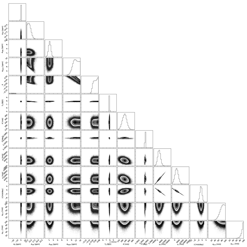
Figure 6: Corner plot of the joint posterior parameter distributions for KIC 8121913.

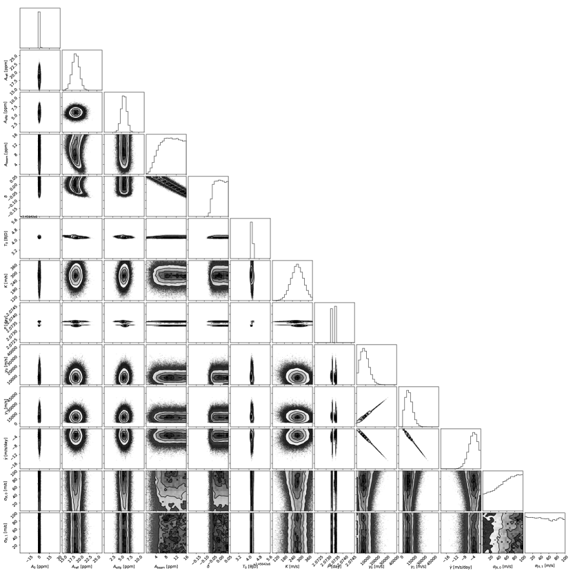
Figure 7: Corner plot of the joint posterior parameter distributions for KIC 10068024.

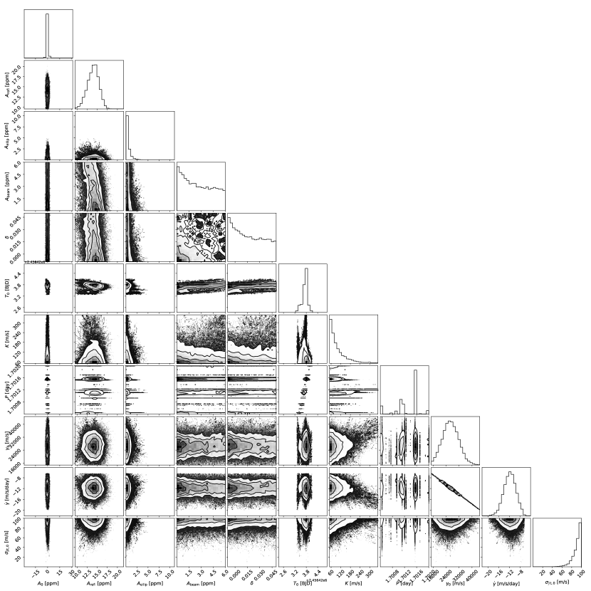
Figure 8: Corner plot of the joint posterior parameter distributions for KIC 5479689.