Theory of the line shape of the 1S–2S transition for magnetically trapped antihydrogen

Abstract

The physics that determines the line shape of the 1S–2S transition in magnetically trapped $\bar{\rm H}$ is explored. Besides obtaining an understanding of the line shape, one goal is to replace the dependence on large scale simulations of $\bar{\rm H}$ with a simpler integration over well defined functions. For limiting cases, analytic formulas are obtained. Example calculations are performed to illustrate the limits of simplifying assumptions. We also describe a $\chi^{2}$ method for choosing experimental parameters that can lead to the most accurate determination of the transition frequency.

I Introduction

One of the main goals of the ALPHA collaboration has been to measure the 1S–2S transition in antimatter hydrogen, $\bar{\rm H}$,Ahmadi and others (ALPHA collaboration, ALPHA collaboration) with an accuracy comparable to that in normal matter H.Parthey et al. (2011) The motivation is to compare these two values as a test of the CPT theoremKosteleckỳ and Russell (2011); one consequence of the CPT theorem is that the transition frequencies of $\bar{\rm H}$ and normal hydrogen should be identical. The frequency in normal matter H is known to an accuracy of a few Hz.Parthey et al. (2011) Currently, this transition frequency is known to an accuracy of a few kHz in $\bar{\rm H}$Ahmadi and others (ALPHA collaboration) which is an excellent achievement considering the few number of $\bar{\rm H}$ in the experiment and the fact that the transitions occur in a magnetic trap which shifts the $\bar{\rm H}$ energies.

The transition frequency in the ALPHA experiments is obtained by comparing the measured line shape to that obtained from a large scale simulation of the $\bar{\rm H}$ trajectories in the modeled magnetic fields. The trajectories are needed to understand the positions where the $\bar{\rm H}$s cross the 243 nm beam and their velocities when crossing. This information is used to solve for the time dependence of the $\bar{\rm H}$ electronic states which is used to compute the transition probability for each crossing. A Monte Carlo sampling of the trajectories then gives the transition probability and the probability the transition can be detected. This simulation is a necessary, but somewhat opaque, step in the comparison of the measured 1S–2S line shape to what is expected assuming CPT. It is likely that the next generation of experiments will lead to data giving an accuracy of a few 100 Hz or better. A few obvious changes will lead to this improved accuracy: smaller power for the 243 nm laser to reduce the AC Stark shift, larger 243 nm waist to decrease transit broadening, colder $\bar{\rm H}$Donnan et al. (2013); Baker and others (ALPHA collaboration) to decrease transit broadening, and more $\bar{\rm H}$ to decrease the statistical error bars on the line.

The purpose of this paper is to examine the physics that determines the line shape of the 1S–2S transition in magnetically trapped $\bar{\rm H}$. One of the goals is to clarify the role different properties of the $\bar{\rm H}$ play in the line shape. Another goal is to explain most aspects of the line shape using analytic formulas that arise in simplified limits and to show how the large scale simulations approach these analytic formulas. A final goal is to explore a $\chi^{2}$ method for predicting how choices for experimental parameters affect the uncertainty in the frequency measurement.

This paper is organized as: Sec. II contains a description of the basic physics determining the line shape, Sec. III contains a description of how to calculate the transition probability for one $\bar{\rm H}$ crossing of the 243 nm beam, Secs. IV (V) contain descriptions for the line shape when the shifts of the frequency due to a change in the magnetic field are not (are) included, Sec. VI contains a description of a method for using $\chi^{2}$ to choose the experimental parameters that would give the most accurate frequency determination, and Sec. VII contains a summary of the results.

II Basic physics of the 1S–2S transition

II.1 Excitation

The two photon absorption from counter-propagating laser beams gives a transition from the 1S to the 2S state with no first order Doppler shift. Because the lifetime of the 2S state in zero electric and magnetic fields is $1/8.2$ s, external factors (e.g. laser waist and power, $\bar{\rm H}$ temperature, magnetic fields, etc) mainly determine the line shape of the 1S–2S transition. This section sketches how to incorporate these effects.

We assume that a Gaussian beam well approximates the light in the trap. If this assumption is violated, most of the analytic results below will no longer be accurate, but the results from solving the optical Bloch equations can incorporate different laser shapes. For a description of a Gaussian beam, we will take the $z$ direction to be along the beam with the $x,y$ directions perpendicular to the beam. The intensity at the center of one beam is $I_{0}=2P_{0}/(\pi w^{2}_{0})$ where $P_{0}$ is the power in the beam and $w_{0}$ is the beam waist. The position dependent intensity for a single Gaussian beam is

$$I(r,z) = I_{0}[w_{0}/w(z)]^{2}\exp[-2r^{2}/w^{2}(z)]$$ (1)

$$w^{2}(z) = w_{0}^{2}(1+z^{2}/Z_{R}^{2})$$ (2)

where $r^{2}=x^{2}+y^{2}$ and the Rayleigh range $Z_{R}=\pi w_{0}^{2}/\lambda$. For the 1S–2S transition, $\lambda=243$ nm. For counterpropagating beams, the electric field at a position $r,z$ is $E=E_{0}[w_{0}/w(z)]\exp[-r^{2}/w^{2}(z)]\cos[\phi(r,z)+\delta]\cos(\omega_{L}t)$ which has the form of a standing wave; the spatial phase dependence, $\phi(r,z)$, is not relevant for our results. The relationship between $E_{0}$ and the one beam maximum intensity is $E_{0}^{2}=8I_{0}/(\varepsilon_{0}c)$.

The theory for this transition has been discussed in several places; we will follow the treatment in Ref. Rasmussen et al. (2017). The coupling of the 1S and 2S states proceeds through a virtual transition to the bound $nP$ and continuum $\mathcal{E}p$-states. After adiabatically eliminating the $p$-states, the equations governing the two-photon coupling between the 1S and 2S states are

$$\frac{dC_{1S}}{dt} =\frac{\xi E_{0}^{2}w_{0}^{2}}{i\hbar w^{2}}e^{-2r^{2}(t)/w^{2}}e^{-i(\mathcal{E}_{2S}-\mathcal{E}_{1S}-2\hbar\omega_{L})t/\hbar}C_{2S}$$ (3)

$$\frac{dC_{2S}}{dt} =\frac{\xi E_{0}^{2}w_{0}^{2}}{i\hbar w^{2}}e^{-2r^{2}(t)/w^{2}}e^{i(\mathcal{E}_{2S}-\mathcal{E}_{1S}-2\hbar\omega_{L})t/\hbar}C_{1S}$$ (4)

where $\omega_{L}=2\pi f_{L}$ is the angular frequency of the laser with $f_{L}$ the laser frequency. and $\mathcal{E}_{2S}-\mathcal{E}_{1S}$ is the energy difference between the 1S and 2S states at the position of the crossing. We will use $f$ in all expressions for frequency. Instead of computing $\xi$ by summing over the infinite number of $nP$ states and integrating over the continuum $\mathcal{E}p$-states, we perform the calculation with the atom inside a spherical box so that the number of negative energy states is finite and the continuum is discretized. If the radius of the box is sufficiently large, $\xi$ is independent of the value of the radius. The parameter $\xi$ is

$$\xi=-\frac{e^{2}}{8}\sum_{n}\frac{D_{2S,nP}D_{nP,1S}}{\mathcal{E}_{nP}-\mathcal{E}_{1S}-\hbar\omega_{L}}\simeq 12.3\varepsilon_{0}a_{0}^{3},$$ (5)

where $a_{0}$ is the Bohr radius, $D_{2S,nP}D_{nP,1S}=\sum_{m}\langle 2S|\vec{r}|nPm\rangle\cdot\langle nPm|\vec{r}|1S\rangle$, with $m$ the azimuthal quantum number, and $e$ is the electric charge. The numerical value was obtained by performing the sum using $nP$ states whose radial wave function is zero at 30$\,a_{0}$.

There are several effects that are missing from these equations which will be added or discussed below. The main missing effects are: the AC Stark shift which arises because the 1S and 2S states have different AC polarizabilities, the second order Doppler shift proportional to the kinetic energy over the rest energy of the $\bar{\rm H}$, ionization of the 2S state by a third photon, radiative decay from the 2S state, mixing of the 2S and 2P states due to the $v\times B$ effective electric field, etc.

The transition frequency depends on the spin coupling of the positron and antiproton and the magnetic field. The 1Sc,2Sc states have total angular momentum 0 in the $B$-field direction while the 1Sd,2Sd states have the two spins antiparallel to the $B$-field direction. Because the 1Sc–2Sc transition has a $\sim 10\times$ larger variation with $B$ when $B\sim 1$ T, we will restrict the examples to the 1Sd–2Sd transition. The change in frequency with $B$ is given byRasmussen et al. (2017)

$$\frac{d\;\hbox{}}{dB}\frac{\mathcal{E}_{2S}-\mathcal{E}_{1S}}{2h}=(\frac{1}{2}186.071+387.678\,B)\;{\rm kHz}$$ (6)

for $B$ in Tesla. The second term is from the diamagnetic term in the Hamiltonian and causes, at larger $B$, a larger variation of the transition frequency with $B$.

Another shift can occur due to a $v\times B$ effective electric field causing an interaction of the 2S with the 2P states. Using Eq. (43) of Ref. Rasmussen et al. (2017), this shift is

$$\Delta{\cal E}_{2S}/h\sim 0.041\;v_{\perp}^{2}\;{\rm Hz}$$ (7)

when $B\sim 1$ T and the perpendicular velocity, $v_{\perp}$, is in $m/s$. For a $\bar{\rm H}$ with a perpendicular kinetic energy of 50 mK, this shift corresponds to $\sim 40$ Hz which is negligible for the next level of accuracy in ALPHA experiments. This shift can be decreased by cooling the $\bar{\rm H}$s.

II.2 Detection

There are several processes that lead to transitions out of the 2S state which can be used to detect the excitation. Ordinary matter experimentsParthey et al. (2011) detect photons emitted after excitation to the 2S state. Detecting emitted photons is probably unfeasible for $\bar{\rm H}$ which is trapped in a long tube. Therefore, other processes are important for detection of the 1S–2S transition in the ALPHA experiments.

Two processes are presumed to dominate the detection in experiments reported previously.Ahmadi and others (ALPHA collaboration, ALPHA collaboration) The first is ionization of the 2S state by a third 243 nm photon. This can occur during the excitation process itself or when an excited $\bar{\rm H}$ recrosses the 243 nm beam at a later time. The second is when the $v\times B$ effective electric field causes mixing with 2P states where the positron has the untrapped spin orientation. This allows a one photon emission back to the ground state into magnetically untrapped 1S states. Both of these processes result in annihilation on the trap wall as the detection step. Unfortunately, both depend on the perpendicular speed of the $\bar{\rm H}$ to some extent which affects the measurement of the transition line shape. However, we will argue below that future experiments should use substantially lower 243 nm laser power and colder $\bar{\rm H}$s to achieve higher precision in the frequency measurement. In this case, neither of these mechanisms will be effective: the ionization is proportional to the laser power and the spin flip is proportional to the temperature.

One possibility is to impose a weak electric field which would cause mixing between the 2S and 2P states. This can lead to a spin flip after a one photon decay back to the ground state. If the electric field were larger than $|v\times B|$, then the decay would be relatively independent of the $\bar{\rm H}$ position and velocity distribution. Another possibility is to stimulate transitions from the 2S to the 2Pf state using microwaves. The 2Pf state has a large probability to decay to untrapped 1S states which lead to annihilation on the trap walls. Microwave intensity of $\sim 0.01-0.1$ mW/cm² would be sufficient to make it the dominant decay process. More importantly, the transition rate will be nearly independent of the $\bar{\rm H}$ velocity and position distribution. Only when the $\bar{\rm H}$ travels to regions of higher $B$-field will the transition rate change because the frequency of the microwave transition depends on $B$. However, most of the $\bar{\rm H}$ trap has nearly the same $B$-field which is why this transition will not strongly depend on the $\bar{\rm H}$ distribution. Thus, a benefit of both detection methods is that the transition line shape is not distorted by the detection process.

III Transition probability for one beam crossing

In this section, we give the expressions for the probability for a transition into the 2S state when the $\bar{\rm H}$ crosses a Gaussian beam of intensity $I(z)$. Because the beam has a finite width, there is a finite time for the $\bar{\rm H}$ to cross the beam, leading to a line width (transit broadening) roughly the inverse of the time to cross the beam. The material in this section briefly summarizes the derivation in Ref. Rasmussen et al. (2017).

III.1 Perturbative expression

When the laser is weak enough, saturation of the transition, the AC Stark shift, and ionization out of the 2S state are negligible effects. If the atom crosses the laser beam quickly enough, the radiative decay of the 2S state can also be neglected. In this case, setting $C_{1S}=1$ in Eq. (4) is a good approximation and an integral over time will give the amplitude to transition to the 2S state.

We are interested in the case where the beam waist is much smaller than the scale over which the magnetic and electric fields vary substantially. This will lead to a position dependent detuning which we define through $\hbar\Delta\equiv 2\hbar\omega_{L}-(\mathcal{E}_{2S}-\mathcal{E}_{1S})$ with the 1S and 2S energies evaluated at the point where the $\bar{\rm H}$ crosses the beam. Given these conditions, the $\bar{\rm H}$ will have nearly constant velocity so that $r^{2}(t)=b^{2}+v_{\perp}^{2}t^{2}$ with $b$ the distance of closest approach to the beam axis and $v_{\perp}$ the magnitude of the velocity perpendicular to the beam axis. The resulting integral is the Fourier transform of a Gaussian which leads to the probability for a transition:

$$|C_{2S}|^{2}\simeq 32\pi\frac{\xi^{2}I_{0}^{2}}{\hbar^{2}\varepsilon_{0}^{2}c^{2}}\frac{w_{0}^{4}}{w^{2}v_{\perp}^{2}}e^{-4b^{2}/w^{2}}e^{-[2\pi w\Delta f/v_{\perp}]^{2}}$$ (8)

where $\Delta f=f_{L}-f_{0}$ with $f_{0}=(\mathcal{E}_{2S}-\mathcal{E}_{1S})/(2h)$ and the waist, $w$, evaluated at the distance of closest approach. In all expressions, the $z$ dependence of the intensity and waist, $I(z),w(z)$ in Eqs. (1) and (2), will not be explicitly written for notational convenience. If the laser has a substantial linewidth, this expression needs to be convolved with the frequency distribution of the laser as in Eq. (32) of Ref. Rasmussen et al. (2017). We will assume this is a small fraction of the width due to the finite crossing time and not include the linewidth of the laser below.

III.2 Optical Bloch equation

In the previous section, we made several assumptions that could affect the line shape. This section will give the equations that can be solved for a more accurate calculation of the transition probability. We follow the derivation of Ref. Rasmussen et al. (2017) by using the density matrix formalism to describe the evolution of the electronic states of the $\bar{\rm H}$, Fig. 1. We only include 4 states in this treatment: $|1\rangle$ is the low field (trappable) 1S state which initially has 100% of the population, $|2\rangle$ is a high field (untrappable) 1S state which can be produced in decays from the 2S state, $|3\rangle$ represents photo-ionization which results when the 2S state absorbs a third photon, and $|4\rangle$ is the low field (trappable) 2S state which is reached in the two photon transition from the 1S state. Properly speaking, $|3\rangle$ is not a state but a continuum of states, Ep; approximating photoionization as decay to a single state can be used because we are only interested in the total population of ionized atoms and it only enters the density matrix equation through decay terms.

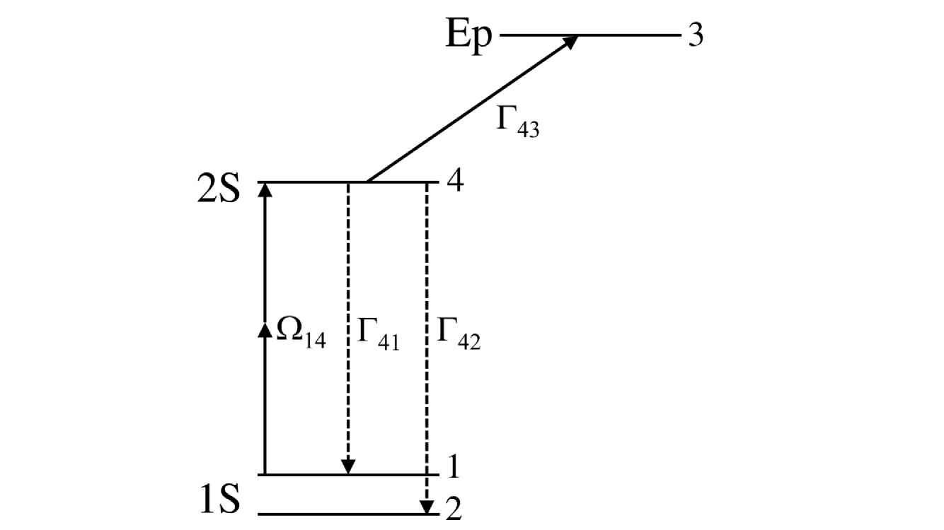
Figure 1: Schematic of the excitation out of the trappable 1S-state $|1\rangle$ into the trappable 2S-state $|4\rangle$. The 2S-state population can decay by photon emission into the 1S-states and by absorption of a third 243 nm photon into the $p$-continuum, $|3\rangle$.

The density matrix equations are written in Lindblad form

$$\frac{d\hat{\rho}}{dt}=\frac{1}{i\hbar}[\hat{H},\hat{\rho}]+\mathcal{L}(\hat{\rho})$$ (9)

which leads to the following equations for the non-zero matrix elements of $\hat{\rho}$:

$$\dot{\rho}_{11} = -\frac{i}{2}\Omega_{14}(t)\left(\rho_{41}-\rho_{14}\right)+\Gamma_{41}\rho_{44}$$

$$\dot{\rho}_{22} = \Gamma_{42}\rho_{44}$$

$$\dot{\rho}_{33} = \Gamma_{43}\rho_{44}$$ (10)

$$\dot{\rho}_{44} = -\frac{i}{2}\Omega_{14}(t)\left(\rho_{14}-\rho_{41}\right)-\Gamma\rho_{44}$$

$$\dot{\rho}_{14} = -\frac{i}{2}\Omega_{14}(t)\left(\rho_{44}-\rho_{11}\right)+\left(-i\Delta_{AC}-\frac{1}{2}\Gamma\right)\rho_{14}$$

where $\Delta_{AC}=\Delta-2\pi\Delta f_{\rm AC}(t)$ and $\rho_{41}=\rho_{14}^{*}$ determines the last non-zero element. The $\Gamma_{4i}$ are the decay rates to the different final states, $\Gamma$ is the sum of these rates, and $\Omega_{14}$ is the two-photon Rabi frequency. The two beam AC Stark shift frequency for the 1S–2S transition is

$$\Delta f_{\rm AC}(t)=2I\textup{e}^{-2r^{2}(t)/w^{2}}1.67\;{\rm Hz}$$ (11)

where $I$ is the intensity of one beam at $z$ and $r=0$ in ${\rm W/cm^{2}}$ and the factor $1.67$ Hz is from Ref. Haas et al. (2006). For two counterpropagating 1 W beams with 200 $\mu$m waist, the $\Delta f_{\rm AC}\approx 5$ kHz. The two photon Rabi frequency is

$$\Omega_{14}(t)=\frac{16\xi I}{\hbar\varepsilon_{0}c}\textup{e}^{-2r^{2}(t)/w^{2}}.$$ (12)

The total decay rate of the 2S state is $\Gamma=\Gamma_{41}+\Gamma_{42}+\Gamma_{43}$ where $\Gamma_{41},\Gamma_{42}$ is the radiative decay rate into the trapable and untrapable 1S states, respectively; see Ref. Rasmussen et al. (2017) for these decay rates. If a microwave or static electric field is causing transitions from the 2S to the 2P states, then the $\Gamma_{41},\Gamma_{42}$ will be increased by factors depending on the strength and detuning of the microwaves or the strength and direction of the electric field. Finally, the ionization rate out of the 2S state is

$$\Gamma_{43}=I\textup{e}^{-2r^{2}(t)/w^{2}}7.57\;\textup{s}^{-1}$$ (13)

where $I$ is in ${\rm W/cm^{2}}$ and the 7.57 was determined by numerically solving for the photo-ionization cross section out of the 2S state from 243 nm photons. For two counterpropagating 1 W beams with 200 $\mu$m waist, the $\Gamma_{43}\approx 2\pi\;4$ kHz.

In the calculations below, we numerically solve the density matrix equations using $I(t)$ and $r(t)$ for individual atom trajectories.

IV Line shape: no magnetic or electric fields

In this section, we give results when the shifts in transition frequency due to external $E$- and $B$-fields are ignored. The perturbative transition rate can be analytically calculated for a thermal distribution of $\bar{\rm H}$ velocity as well as for an equal distribution of velocities within a sphere in velocity space. The perturbative transition rate can be reduced to a single integral when the distribution only depends on the $\bar{\rm H}$ kinetic energy.

IV.1 Perturbative result

For this section, we use the perturbative calculation of the transition probability for one beam crossing, Eq. (8), as the starting point. We then average over the $\bar{\rm H}$ positions and velocities to get the rate for transition into the 2S state. To simplify the notation, we will combine the terms in the probability that do not contain $v_{\perp}$ or $b$ into

$$A\equiv 32\pi\frac{\xi^{2}I_{0}^{2}}{\hbar^{2}\varepsilon_{0}^{2}c^{2}}\,\frac{w_{0}^{4}}{w^{2}}.$$ (14)

The rate that $\bar{\rm H}$s pass the beam with a distance between $b$ and $b+db$ is

$${\cal F}=\rho_{2D}v_{\perp}2db$$ (15)

where the $\rho_{2D}$ is the two-dimensional $\bar{\rm H}$ density and the 2 arises because the $\bar{\rm H}$ can pass on either side of the beam for a given direction $\hat{v}_{\perp}$. The probability distribution for finding an $\bar{\rm H}$ with a perpendicular speed between $v_{\perp}$ and $v_{\perp}+dv_{\perp}$ will be called $v_{\perp}{\cal D}(v_{\perp})dv_{\perp}$.

The rate of $\bar{\rm H}$s transitioning from the 1S to the 2S state divided by the two-dimensional $\bar{\rm H}$ density is

$${\cal G} = 2A\int_{0}^{\infty}e^{-4b^{2}/w^{2}}db\int_{0}^{\infty}{\cal D}(v_{\perp})e^{-[2\pi w\Delta f/v_{\perp}]^{2}}dv_{\perp}$$ (16)

$$= \frac{Aw\sqrt{\pi}}{2}\int_{0}^{\infty}{\cal D}(v_{\perp})e^{-[2\pi w\Delta f/v_{\perp}]^{2}}dv_{\perp}$$

Note that the ${\cal G}$ has units of $area/time$.

We note that this expression is somewhat problematic for small $\Delta f$ because the perturbation calculation of the transition probability has a factor of $1/v_{\perp}^{2}$ which can cause $|C_{2S}|^{2}$ to be larger than 1 for small $\Delta f$ which is impossible. Thus, the perturbative calculation of the line shape will be inaccurate for small detuning. The range of detuning where the line shape is inaccurate decreases as the intensity decreases.

IV.1.1 Thermal distribution

The results in this section reproduce those in Ref. Biraben et al. (1979) for the special case of equal intensity in the counter-propagating beams. The distribution of $v_{\perp}$ for a thermal distribution is ${\cal D}_{th}=(2/v_{th}^{2})\exp(-v_{\perp}^{2}/v_{th}^{2})$ with $v_{th}^{2}\equiv 2k_{B}T/M$ with $T$ the temperature and $M$ the mass of the $\bar{\rm H}$. The thermal transition rate into the 2S state is

$${\cal G}_{th} = \frac{Aw\sqrt{\pi}}{v_{th}^{2}}\int_{0}^{\infty}\exp\left[-\frac{v_{\perp}^{2}}{v_{th}^{2}}-\frac{(2\pi w\Delta f)^{2}}{v_{\perp}^{2}}\right]dv_{\perp}$$ (17)

$$= \frac{\pi Aw}{2v_{th}}e^{-|f_{L}-f_{0}|/\phi}$$

where $\phi=v_{th}/(4\pi w)$ which gives a linewidth proportional to $v_{th}/w$ as expected (although the exponential of the absolute value of the detuning is an interesting functional form).

Because the perturbative calculation is problematic for small detuning, we expect the transition rate to be modified for $f_{L}\simeq f_{0}$. Therefore, the discontinuous change in slope of ${\cal G}_{th}(f_{L})$ with respect to the laser frequency will be modified for the actual transition.

When the $\bar{\rm H}$s are in a trap, the $v_{\perp}$ distribution, ${\cal D}(v_{\perp})$, must exactly go to zero for energies that can escape the trap. Therefore, the thermal distribution will only be relevant for $k_{B}T$ much less than the trap energy. For the reported ALPHA experimental results, the $\bar{\rm H}$ trap depth is $E/k_{B}\sim 1/2$ K.

IV.1.2 Energy dependent distribution

The next case we consider is when the $v_{\perp}$ distribution arises from a distribution with respect to energy in 3D with the velocity in the $z$-direction averaged out. In this case, the ${\cal D}(v_{\perp})$ will be a function of $v_{\perp}^{2}$. For a general case, the integral in Eq. (16) needs to be performed numerically. Although the essential singularity at $v_{\perp}=0$ looks bad, the integrals over one parameter can be evaluated by simply increasing the number of points.

As an example that can be done analytically, consider the early ALPHA experiments where the distribution of $\bar{\rm H}$s could be considered as the low energy portion of a high temperature distribution. As an extreme example, we consider the case where the velocity distribution is flat in $v_{x},v_{y},v_{z}$ up to the condition $v_{m}^{2}>v_{x}^{2}+v_{y}^{2}+v_{z}^{2}$; this is a flat distribution within a sphere in velocity space. This gives ${\cal D}_{m}=3\sqrt{v_{m}^{2}-v_{\perp}^{2}}/v_{m}^{3}$. Using this distribution, the transition rate in units of $area/time$ is

$${\cal G}_{m} = \frac{Aw\sqrt{\pi}3}{2v_{m}}\int_{0}^{1}\sqrt{1-s^{2}}\;e^{-\eta^{2}/s^{2}}ds$$ (18)

$$= \frac{3Aw\pi\sqrt{\pi}}{8v_{m}}\left[(2\eta^{2}+1){\rm erfc}(|\eta|)-\frac{2|\eta|}{\sqrt{\pi}}e^{-\eta^{2}}\right]$$

where $\eta=2\pi w(f_{L}-f_{0})/v_{m}$. As with the previous section, this expression will be least accurate for $f_{L}\simeq f_{0}$ but will become accurate over a larger range as the laser intensity decreases.

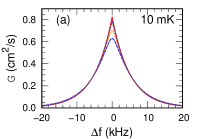
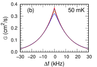
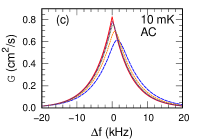
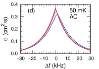
Figure 2: The thermally averaged 1S–2S transition rate. All results use a beam waist of 200 $\mu$m and don’t include magnetic and electric field shifts versus detuning of the two photon transition. The results are all scaled by a factor of $1/P_{0}^{2}$ with $P_{0}$ the power in one beam so that the lines are on the same scale for different powers. The perturbative treatment, Eq. (17), (red solid line) does not change with intensity. The optical Bloch results change with power: 1 W (blue dashed), 0.5 W (orange short dash), 0.2 W (green dotted), and 0.1 W (purple dash-dot). (a) and (c) are for 10 mK thermal distribution (b) and (d) are for 50 mK thermal distribution. Plots (c) and (d) include the AC Stark shift in the optical Bloch equations while (a) and (b) do not.

IV.2 Optical Bloch result

Because this section only investigates the excitation of the 2S state, we will set the branching ratio of the radiative decay to be 100% into the untrapped 1S state. With this condition, the excitation rate divided by the two-dimensional $\bar{\rm H}$ density is

$${\cal G}_{ob}=\int_{0}^{\infty}\int_{0}^{\infty}2v_{\perp}^{2}{\cal D}(v_{\perp})(1-\rho_{11})dbdv_{\perp}$$ (19)

where the density matrix element, $\rho_{11}$ is evaluated at large time for parameters $b$ and $v_{\perp}$.

IV.2.1 Thermal distribution

In this section, we present results from numerically solving the optical Bloch equations and using the result to calculate the rate, ${\cal G}$. We solved the optical Bloch equations, Eq. (III.2), using equal steps in $db$ to sample the crossing distance, $b$, and equal steps in $dv_{\perp}$ to sample the perpendicular speeds, $v_{\perp}$. From above, the thermal distribution gives ${\cal D}(v_{\perp})=(2/v_{th}^{2})\exp(-v_{\perp}^{2}/v_{th}^{2})$ in Eq. (19). We performed calculations for two temperatures, 10 and 50 mK, and laser powers from 0.1 to 1 W to illustrate the limitation of the perturbative line shape, Eq. (17).

In order to more easily compare the results for different laser powers, we scaled the ${\cal G}$ by dividing by the squared laser power. The calculations were done for a 200 $\mu$m waist and do not include shifts from the electric or magnetic field in order to emphasize the effects from the AC Stark shift and the saturation of the transition. Calculations were done for 0.1, 0.2, 0.5, and 1.0 W of power in each beam. The results are shown in Fig. 2 where we have suppressed the AC Stark shift in (a) and (b) but shown the full results in (c) and (d).

There are a few important trends that are worth noting. For the calculations that suppressed AC Stark shift, Figs. 2(a) and (b), only saturation of the 1S–2S is changing the results from perturbation theory, Eq. (17). The decay of the atom while crossing the beam has a minor effect for the parameters of these calculations. As foreshadowed above, saturation is more important for slowly moving atoms which are the ones that mainly contribute to the signal near zero detuning. The region of detuning where the optical Bloch differs from the perturbative results decreases with decreasing laser power. Unsurprisingly, saturation is more important for the 10 mK $\bar{\rm H}$s than for those at 50 mK due to the larger fraction of slow atoms. The AC Stark shift in Figs. 2(c) and (d) is the other important effect in these calculations. The size of the shift is approximately the same for the two temperatures because it depends on the path through the laser beam and not the time in it. However, the size of the shift is a factor of $\sim 3.5$ smaller than the estimate from Eq. (11). For example, at 1 W, the peak in Figs. 2(c) and (d) are shifted by 1.5 kHz compared to 5.3 kHz from Eq. (11). The actual shift is smaller because the 5.3 kHz is the shift at the intensity maximum whereas the $\bar{\rm H}$s travel through the beam, experiencing both large and small intensity, and they always miss the exact center when they cross the beam so the peak intensity on a particular crossing is less than the maximum.

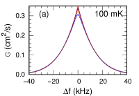
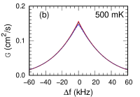
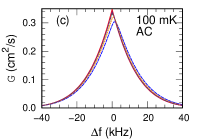
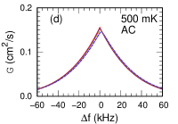
Figure 3: Same as Fig. 2 except for a flat velocity distribution up to the limit $|\vec{v}|=v_{m}$ with $(1/2)Mv_{m}^{2}/k_{B}=100$ mK for (a) and (c) and 500 mK for (b) and (d).

IV.2.2 Energy dependent distribution

The results in this section are for the case where there is a flat velocity distribution within a sphere in velocity space of radius $v_{m}$ and zero otherwise. This gives ${\cal D}=(3/v_{m}^{3})\sqrt{v_{m}^{2}-v_{\perp}^{2}}$ as discussed above. As with the previous section, we numerically solve the optical Bloch equations to obtain $\rho_{11}$ and use Eq. (19) to calculate the rate.

These results are compared to the analytic, perturbative expression, Eq. (18), in Fig. 3. For this case, we have somewhat higher $\bar{\rm H}$ energies than the previous section because previous experiments, Ref. Ahmadi and others (ALPHA collaboration, ALPHA collaboration), have a trap depth of $\sim 1/2$ K which matches Figs. 3(b) and (d). The shape of the rate versus frequency is qualitatively similar to the previous results. There is a similar cusp feature for the calculations that do not include the AC Stark shift, Figs. 3(a) and (b). As with the previous section, the AC Stark shift, Figs. 3(c) and (d), gives a $\approx 1.5$ kHz displacement of the peak position for 1 W power in one beam.

The width for the 100 mK case in Fig. 3 has approximately the same width as the 50 mK in Fig. 2, within 10%. This is because the flat distribution within a sphere is missing the higher energy $\bar{\rm H}$’s which broaden the line. Although the line shapes are similar, the thermal distribution falls faster at smaller detunings and then slower at larger detuning reflecting the difference in shape of a thermal and a flat distribution with respect to speed.

V Line shape: nonzero magnetic shift

In this section, we give results when the shifts in transition frequency due to magnetic fields are included. The perturbative transition rate can be calculated analytically for a thermal distribution and power law potential and reduced to a single integral for a distribution which is equally likely for energy less than a limit. If the distribution only depends on the energy, the perturbative transition rate can be reduced to a two dimensional integral.

The main idea in this section is that the probability for crossing the beam at a position, $z$, depends on the trapping fields and will be represented by a probability distribution of the $\bar{\rm H}$’s, ${\cal P}(z)$. The shift in the transition frequency depends on the magnetic field at the position $z$ as well. By convolving these effects with the transition rate as a function of $z$, the overall transition rate, ${\cal J}$, can be calculated. As with the previous section, the ${\cal J}$ will have units of $area/time$.

If the $v_{\perp}$ distribution does not depend on $z$, then the transition rate only has a $z$ dependence through the transition frequency, $f_{0}(z)$: ${\cal G}(f_{L}-f_{0}(z))$. There are distributions where the $v_{\perp}$ distribution does depend on $z$ in which case we will indicate the extra parametric dependence as ${\cal G}(f_{L}-f_{0}(z),z)$. An example of this is a distribution which is flat in velocities and $z$ for $E<E_{m}$ and zero for $E>E_{m}$. The overall transition rate is then

$${\cal J}=\int{\cal G}(f_{L}-f_{0}(z),z){\cal P}(z)dz$$ (20)

where the integral is over the region where ${\cal P}(z)$ is nonzero.

V.1 Perturbative result

For weak lasers where the perturbative result is accurate, the rate can be calculated from Eq. (16) when given the $v_{\perp}$ distribution, ${\cal D}(v_{\perp})$, at the position $z$. For the two special cases treated in the figures above, analytic expressions, Eqs. (17) and (18), are available. For a general position distribution, ${\cal P}(z)$, and magnetic field, $B(z)$, the overall transition rate will result from a one-dimensional integration, Eq. (20).

For the next two subsections, we assume that the magnetic field has a simple form

$$B(z)=B_{0}+B_{\nu}z^{\nu}$$ (21)

with $\nu$ an even integer to give an effective potential energy that traps the $\bar{\rm H}$ in $z$. In Sec. V.2.3, we discuss more physical magnetic fields.

V.1.1 Thermal distribution: power law potential and shift

In this section, we assume the $\bar{\rm H}$ distribution is from a thermal distribution in velocity and position. In this case, the $v_{\perp}$ distribution is independent of $z$ resulting in the transition rate in Eq. (17). The position distribution is

$${\cal P}_{th}(z)=Ce^{-\beta\mu B_{\nu}z^{\nu}}$$ (22)

where $\mu$ is the magnetic dipole moment of the 1Sd state, $C=\nu(\beta\mu B_{\nu})^{1/\nu}/[2\Gamma(1/\nu)]$, $\beta=1/(k_{B}T)$ and $\Gamma(z)$ is the Gamma function. Because $\mu$ will always be multiplied by $\beta$, which typically won’t be very well known, the magnetic dipole moment of the electron can be used. The constant in front of the exponential gives a normalized position distribution. In terms of $z$, the transition frequency versus $z$ can be found from Eq. (6) to give

$$f_{0}(z)=f_{0}(0)+f_{\nu}z^{\nu}+f_{2\nu}z^{2\nu}$$ (23)

where $f_{0}(0)$ is the frequency evaluated at $B=B_{0}$, $f_{\nu}=(93.035+387.678B_{0})B_{\nu}$ kHz, and $f_{2\nu}=193.839B_{\nu}^{2}$ kHz where $B_{0}$ is in Tesla and $B_{\nu}$ is in Tesla/meter^ν (to avoid the symbol $T$ which could be confused with temperature). Putting together with Eq. (17), the overall transition rate is

$${\cal J}_{th}=\frac{\pi AC}{2v_{th}}\int_{-\infty}^{\infty}we^{-|\Delta f-f_{\nu}z^{\nu}-f_{2\nu}z^{2\nu}|/\phi}e^{-\beta\mu B_{\nu}z^{\nu}}dz$$ (24)

where $\phi=v_{th}/(4\pi w)$, $\Delta f=f_{L}-f_{0}(0)$, and the $z$-dependence of the waist, $w(z)$, is from Eq. (2). For the typical cases in the ALPHA experiment, the waist is 200 $\mu$m giving $Z_{R}=0.52$ m. The $z$-dependence in the waist will lead to errors of $\sim$1% in ${\cal J}$ and, therefore, we will ignore this dependence. Even with this approximation, we have not found an analytic expression for Eq. (24) and evaluated it numerically.

For low temperatures, the $\bar{\rm H}$ can not reach magnetic fields substantially larger than $B_{0}$. In this case, the contribution from $f_{2\nu}z^{2\nu}$ is negligible and the integral can be evaluated analytically. For $f_{2\nu}=0$,

$${\cal J}_{th}(\Delta f<0) = \frac{\pi w_{0}A}{2v_{th}}\tau_{+}^{1/\nu}e^{\Delta f/\phi}$$

$${\cal J}_{th}(\Delta f>0) = \frac{\pi w_{0}A}{2v_{th}}\tau_{+}^{1/\nu}\frac{\Gamma(1/\nu,t_{+})}{\Gamma(1/\nu)}e^{\Delta f/\phi}+$$ (25)

$$\frac{\pi w_{0}A}{2v_{th}}\tau_{-}^{1/\nu}\frac{\tilde{\gamma}(1/\nu,t_{-})}{\Gamma(1/\nu)}e^{-\Delta f/\phi}$$

where $\tau_{\pm}=\beta\mu B_{\nu}/[\beta\mu B_{\nu}\pm(f_{\nu}/\phi)]$, $t_{\pm}=[\beta\mu B_{\nu}\pm(f_{\nu}/\phi)]z_{0}^{\nu}$, and $f_{\nu}z_{0}^{\nu}=\Delta f=f_{L}-f_{0}(0)$ defines the position where the detuning is zero. The incomplete gamma functions are defined as

$$\Gamma(s,x)=\int_{x}^{\infty}t^{s-1}e^{-t}dt$$ (26)

while the possibility for $t_{-}<0$ leads to the generalized definition

$$\tilde{\gamma}(1/\nu,t_{-}>0) = \int_{0}^{t_{-}}t^{(1/\nu)-1}e^{-t}dt=\Gamma(1/\nu)-\Gamma(1/\nu,t_{-})$$

$$\tilde{\gamma}(1/\nu,t_{-}<0) = \nu\int_{0}^{t_{-}^{1/\nu}}e^{-u^{\nu}}du$$ (27)

$$= \nu t_{-}^{1/\nu}\sum_{n=0}^{\infty}\frac{(-t_{-})^{n}}{n!(n\nu+1)}$$

where the $1/(\beta\mu B_{\nu}-(f_{\nu}/\phi))^{1/\nu}$ in Eq. (V.1.1) from the $\tau_{-}$ cancels the same term in the $t_{-}^{1/\nu}$ from Eq. (V.1.1) when $t_{-}<0$.

V.1.2 Energy dependent distribution: power law potential and shift

In this section, we examine the case where there is a flat distribution in $v_{x},v_{y},v_{z},z$ with the condition that $E<E_{m}$. This is similar to the condition in Sec. IV.1.2 but accounting for the potential energy along $z$. For this case, we can use the result in Eq. (18) that analytically includes the averaging over impact parameter and $\vec{v}$ in the $z$-convolution, Eq. (20). In this case, the $v_{m}$ depends on $z$: $Mv_{m}^{2}(z)/2=E_{m}-\mu[B(z)-B_{0}]$. The probability distribution is

$${\cal P}_{m}(z)=v_{m}^{3}(z)\left[\int_{z_{0}}^{z_{f}}v_{m}^{3}(z^{\prime})dz^{\prime}\right]^{-1}\;{\rm for}\;z_{0}<z<z_{f}$$ (28)

where the $v_{m}(z_{0})=v_{m}(z_{f})=0$. Using the simplified $B(z)$ from above gives $z_{f}=-z_{0}=[E_{m}/(\mu B_{\nu})]^{1/\nu}$ and

$${\cal P}_{m}(z) = \frac{1}{2z_{f}\;{}_{2}F_{1}(-\frac{3}{2},\frac{1}{\nu};1+\frac{1}{\nu};1)}\left[1-(z/z_{f})^{\nu}\right]^{3/2}$$ (29)

$$= \frac{2\Gamma(\frac{5}{2}+\frac{1}{\nu})}{3\sqrt{\pi}\Gamma(1+\frac{1}{\nu})z_{f}}\left[1-(z/z_{f})^{\nu}\right]^{3/2}$$

Unfortunately, we have not found an analytic expression for the convolution

$${\cal J}_{m}=2\int_{0}^{z_{f}}{\cal G}_{m}(f_{L}-f_{0}(z),z){\cal P}_{m}(z)dz.$$ (30)

However, the average rate can be easily evaluated numerically because it is a one dimensional integral.

V.2 Optical Bloch result

As with Sec. IV.2, the full calculation of the line shape uses the ${\cal G}_{ob}$ from Eq. (19) in the convolution of Eq. (20). The AC Stark shift is included in all of the calculations in this section. For all calculations, we use Eq. (21) with $B_{0}=0.1$ or 1 Tesla and $\nu=6$ with $B_{6}=0.5/0.12^{6}$ Tesla/m⁶. This gives a variation in $z$ very similar to that in the ALPHA trap along the beam axis. To date, the ALPHA experiments have $B_{0}\approx 1$ Tesla.

V.2.1 Thermal distribution

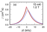
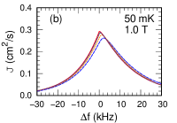
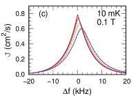
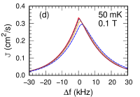
Figure 4: Similar to Fig. 2 except for Eq. (20) which includes the frequency shifts due to a magnetic field of the form $B(z)=B_{0}+B_{6}z^{6}$. The red solid line does not include the AC Stark shift and was computed using Eq. (24). The other line types match the laser powers in Fig. 2. The $B_{0}=1.0$ Tesla are plotted in (a) and (b) while the 0.1 Tesla are in (c) and (d). The $T=10$ mK are in (a) and (c) while the 50 mK are in (b) and (d). All calculations include the AC Stark shift.

We present results, in Fig. 4, from numerically solving the optical Bloch equations for different $\bar{\rm H}$ temperatures and laser powers. In addition, we changed the value of $B_{0}$ from 1.0 Tesla in Figs. 4(a) and (b) to 0.1 Tesla in (c) and (d). These calculations illustrated a few trends that will be important for future measurements.

The frequency shift from the magnetic field breaks the symmetry of the line so that the decrease with positive detuning is slower than for negative detuning. This effect increases with $B_{0}$ because the frequency shift with magnetic field, Eq. (6), increases with $B_{0}$. This leads to larger width for larger $B_{0}$. The increase of $d\Delta E/dB$ with $B$ is due to the diamagnetic term in the Hamiltonian for the 1Sd–2Sd transition. The $d\Delta E/dB$ is roughly four times larger for 1.0 Tesla compared to 0.1 Tesla. Decreasing the magnetic field further gives some decrease in $d\Delta E/dB$, but the effect is not so large: only $\sim$30% change going from 0.1 Tesla to 0 Tesla. As with the calculations in Fig. 2, saturation of the transition and AC Stark shift plays an increasing role in going from 0.1 W to 1.0 W. The saturation causes a suppression in the region of the peak which leads to a more rounded maximum for the line shape at higher power. The AC Stark shift moves the peak position by a somewhat larger amount, $\simeq 1.9$ kHz, possibly due to the slower decrease for positive detuning. Lastly, the $f_{2\nu}$ term in the frequency shift, Eq. (23), did not contribute a noticeable effect to the line shape because the largest effect is for large $z$ where the detuning is large and the transition rate varies slowly with $\Delta f$. Thus, the approximation Eq. (V.1.1) works well for these cases at small power.

V.2.2 Energy dependent distribution

Similar to the previous section, we present results, in Fig. 5, from numerically solving the optical Bloch equations for different $\bar{\rm H}$ cutoff energies and laser powers. In addition, we changed the value of $B_{0}$ from 1.0 Tesla in Figs. 5(a) and (b) to 0.1 Tesla in (c) and (d).

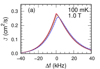
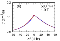
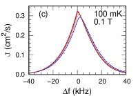
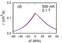
Figure 5: Similar to Fig. 3 except for Eq. (20) which includes the frequency shifts due to a magnetic field of the form $B(z)=B_{0}+B_{6}z^{6}$. The red solid line does not include the AC Stark shift and was computed using Eqs. (30). The other line types match the powers in Fig. 2. The $B_{0}=1.0$ Tesla are plotted in (a) and (b) while the 0.1 Tesla are in (c) and (d). The $E_{m}=100$ mK are in (a) and (c) while the $E_{m}=500$ mK are in (b) and (d). All calculations include the AC Stark shift.

The results in this section hold similar lessons as the previous sections. For example, the magnetic field leads to an asymmetry in the line with the asymmetry increasing with increasing $B_{0}$. The AC Stark shift is somewhat larger than the case for no shift with B-field: $\sim 2$ kHz for 1 W of power. Also, a larger cutoff energy leads to a broader linewidth with the effect somewhat smaller for a thermal distribution at the temperature.

V.2.3 More complex cases

For the ALPHA experiment, the magnetic field does not have the simple power law dependence of the previous sections. Thus, there aren’t simple analytic formulas that can be developed for ALPHA. However, the results in the previous sections point to the possibility that the extensive numerical simulations used in previous studiesAhmadi and others (ALPHA collaboration, ALPHA collaboration) are not necessary. When three conditions are satisfied, the line shape can be determined by integration: 1) the distribution of trajectories is approximately known, 2) the laser is sufficiently weak that AC Stark shifts and depletion of atoms are negligible, and 3) the detection of $\bar{\rm H}$’s do not depend on the frequency, $\Delta f$. The Eqs. (16) and (20) are used with the known spatial dependence of the magnetic field to obtain the line shape. If the AC Stark shifts are non-negligible but there is little depletion of atoms, then the optical Bloch equation can be used so that Eqs. (19) and (20) will give the line shape.

In fact, the Fig. 5(b) is for similar parameters for the ALPHA experiment.Ahmadi and others (ALPHA collaboration, ALPHA collaboration) A comparison with the figures from these papers shows a strong similarity with the 1 W example.

We carried out a calculation for a 50 mK thermal distribution of $\bar{\rm H}$s in the actual ALPHA magnetic fields. We simulated their motion as in Refs. Ahmadi and others (ALPHA collaboration, ALPHA collaboration) and their transition using the optical Bloch equations. The only difference with the usual calculation was artificially setting the detection efficiency to be independent of the $\bar{\rm H}$ position and velocity. We also assumed the $\bar{\rm H}$ population was not depleted which isn’t the case in the experiments. We compared this result to that using the ${\cal G}_{ob}$ from Eq. (19) in the convolution of Eq. (20). We found perfect agreement in this case. This comparison shows our results can be extended to more complex magnetic fields.

VI Optimum parameters

In this section, we discuss how various parameters affect the accuracy of the 1Sd–2Sd frequency measurement. We will first address some of the more obvious parameters (e.g. laser power and waist, uniform $B$-field value, etc.) by discussing the trends in the line width. We will then show that the predicted $\chi^{2}$ is useful for assessing less obvious parameters (e.g. the number of frequencies and their values in a measurement).

To orient the discussion, note the current uncertainty of the $\bar{\rm H}$ 1Sd–2Sd measurement is at the few kHz level. Clearly, the immediate goal is to improve this to the few 100 Hz level with a long term goal to reach the few Hz level.

Laser power: In $\bar{\rm H}$ experiments, the AC Stark shift for 243 nm laser at $\sim 1$ W is 1-2 kHz and is not currently the controlling factor in the uncertainty. To reach uncertainties that are at the few 100 Hz level, the laser power should be decreased by at least an order of magnitude since the AC Stark shift is proportional to the laser power. Also important, high laser power leads to a large fraction of the atoms transitioning to the 2Sd state. Because the transition is detected by $\bar{\rm H}$ that are ejected from the trap, the characteristics of the $\bar{\rm H}$ population (i.e. position and velocity distribution) changes when there is a large probability for a transition. This is problematic because detailed modeling of the population becomes necessary when a substantial fraction of the atoms are ejected.

Laser waist: The line width is mainly from the finite time for an $\bar{\rm H}$ to cross the laser beam, i.e. transit broadening. By doubling the waist, this contribution to the line width will decrease by a factor of 2. This leads to a more accurate determination of the transition frequency.

$\bar{\rm H}$ temperature: At lower temperature, the $\bar{\rm H}$ requires more time to cross the laser beam leading to smaller contribution to the line width from transit broadening. Also, at lower temperature, the $\bar{\rm H}$ can not reach as large $B$-field which also decreases that contribution to the line width. Finally, shifts from the $v\times B$ effective electric field, are proportional to the temperature. Laser cooling of $\bar{\rm H}$ has been demonstratedBaker and others (ALPHA collaboration) as well as the effect on the line width. After laser cooling, trap depths of $\sim 1/2$ K are not necessary. This would allow for a controlled decrease in the depth of the trap. A slowly decreased trap depth leads to adiabatic cooling which further improves the measurements.

Uniform $B$-field: The size of $B_{0}$ affects the line width through the diamagnetic term in the 1S and 2S energies. For larger $B_{0}$, the change in frequency with changing $B$-field is larger which leads to a larger line width. The current experiments typically occur with $B_{0}\sim 1$ T because the plasmas used to make $\bar{\rm H}$ are colder, more stable, and easier to diagnose at large $B_{0}$. It is possible to form $\bar{\rm H}$ at $\sim 1$ T and later ramp $B_{0}$ to lower values. The difficulty with ramping the magnetic field is to precisely know the final value due to persistent currents. Thus, there is incentive to keep $B_{0}\sim 1$ T. Fortunately, from Fig. 4 and 5, although there is a change in the line width in going from $B_{0}=1$ to 0.1 T, the change is less than a factor of 2. Thus, from the perspective of line width, there may not be enough gained by decreasing $B_{0}$.

$\chi^{2}$ treatment: There are other parameters that affect the accuracy of the measured 1Sd–2Sd transition frequency but are not as obvious. For example, given 9 frequencies to measure the transition, which frequencies should be chosen? Or, would it be better to use 9 or 17 frequencies to measure the line? How does the presence of background atoms affect the accuracy of the frequency determination? In these cases, we propose to use the $\chi^{2}$ of a calculated line shape to guide these choices.

For this discussion, we will use the form in Eq. (V.1.1) with the parameters of Fig. 4(b) as the exact transition and will briefly investigate the role played by the frequencies chosen in the measurement. We will have $n_{f}$ frequencies with $\Delta f_{j}$. We will also include the possibility that all transitions are shifted by $\delta f$. We can compute a synthetic line by using Monte Carlo to randomly determine the number of atoms, $N_{j}(\delta f)$, to make a transition at frequency $\Delta f_{j}$ for a fixed total number $N$. On average, this leads to $\bar{N}_{j}(\delta f)$ atoms making the transition with

$$\bar{N}_{j}(\delta f)=N{\cal J}_{th}(\Delta f_{j}+\delta f)/\sum_{j}{\cal J}_{th}(\Delta f_{j}+\delta f)$$ (31)

with $N$ the total number of atoms making the transition. We computed a $\chi^{2}$ by averaging over many different realizations of the Monte Carlo simulation

$$\chi^{2} = \langle\sum_{j}[\bar{N}_{j}(0)-N_{j}(\delta f)]^{2}\rangle/\bar{N}_{j}(0)$$ (32)

$$\simeq n_{f}-1+\sum_{j}[\bar{N}_{j}(0)-\bar{N}_{j}(\delta f)]^{2}/\bar{N}_{j}(0)$$

where the $\langle...\rangle$ on the first line means to average over the different realizations and the second line is from Poisson statistics. Because we fix $N$, the number of degrees of freedom is $n_{f}-1$.

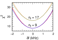
Figure 6: Calculations with 9 frequencies are (red solid) for spacing 1 and (blue dashed) for spacing 1/2. Calculations with 17 frequencies are (orange short dash) for spacing 1 and (green dotted) for spacing 1/2. All calculations were for $N=1000$ transitions.

In Fig. 6, we use the $\chi^{2}$ to see how choices for the frequencies can affect the accuracy for which the transition is determined. Instead of allowing all detunings to be freely varied, we started with a symmetric choice similar to that used in an ALPHA experiment. We did four choices for the frequencies. Spacing 1 for $n_{f}=9$ were the frequencies $\Delta f_{j}=0,\pm 5,\pm 10,\pm 20,\pm 50$ kHz while spacing 1/2 divided every frequency by 1/2. Spacing 1 and 1/2 for $n_{f}=17$ also used the frequencies halfway between those for $n_{f}=9$, i.e. $\Delta f_{j}=0,\pm 2.5,\pm 5,\pm 7.5,...$ kHz. For 8 degrees of freedom, $\chi^{2}\simeq 20$ corresponds to a p-value of 0.01 while this corresponds to $\chi^{2}\simeq 32$ for 16 degrees of freedom. Visually, it is clear that the spacing 1 calculations give slightly greater curvature and therefore modestly better bounds on the uncertainty in the frequency. To compare 9 versus 17 points, the p-value of $\simeq 0.01$ corresponds to $\delta f\simeq-1.5,1.6$ for $n_{f}=9$ and $\delta f\simeq-1.8,1.8$ for $n_{f}=17$ which means the $n_{f}=9$ will give a somewhat better bound on the transition frequency. More importantly, this suggests using $\chi^{2}$ as a metric for choosing the number and values for the frequency.

As a simple extension, we use the ideas of this section to estimate parameters needed to get to few 100 Hz accuracy. If the laser waist is increased from 200 to 400 $\mu$m, the uncertainty decreases by a factor of 2. Increasing the number of detected $\bar{\rm H}$’s from 1,000 to 4,000 decreases the uncertainty by another factor of 2. These two improvements with the estimate from the previous paragraph leads to a few 100 Hz accuracy.

This example is somewhat artificial because the $\bar{\rm H}$ temperature may not be well known even if the distribution is approximately thermal. In this case, the $\chi^{2}$ can be calculated versus $T$ and $\delta f$. We have done this for the $n_{f}=9$, spacing 1 case and found that the $\chi^{2}$ gave $30<T<80$ mK (compared to 50 mK of the actual distribution) with the range of $\delta f$ similar to that found above. This showed that a simultaneous fit could give reasonable results. The example is also artificial in that we did not include the effect of frequency independent background atoms; the background atoms will somewhat increase the uncertainty in the frequency but should not skew the results. Finally, in the real experiment, the detection efficiency could depend on the frequency of excitation, $\Delta f_{j}$, which would skew the results. We have not treated the change in line shape due to detection efficiency but it can be incorporated into our treatment if it is known. These artificial conditions can be easily removed in the numerical implementation of the $\chi^{2}$ method. We have not done so here because they depend on specific aspects of future experiments.

VII Summary

We have examined some of the physics that determines the line shape of the 1Sd–2Sd transition in magnetically trapped $\bar{\rm H}$. Under three assumptions (the distribution of trajectories is approximately known, the laser is sufficiently weak that AC Stark shifts and depletion of atoms are negligible, and the detection of $\bar{\rm H}$’s do not depend on the frequency, $\Delta f$), the line shape can be calculated as an integral over a few degrees of freedom. If the AC Stark shift is not negligible, solutions from optical Bloch equations can be used in these integrals. In either case, large scale, detailed simulations of the trajectories would not be needed to obtain the line shape. We presented analytic expressions for the transition rates for special cases of the $\bar{\rm H}$ distribution and magnetic field.

We discussed several of the trends that control the accuracy with which the transition frequency can be determined. These include parameters such as $\bar{\rm H}$ distribution, laser waist and intensity, uniform $B$-field, number and choice of frequencies sampled, and others. We also propose the use of a $\chi^{2}$ test to optimize the choices for these parameters. From the discussions above, it seems that modest improvements in the ALPHA experiment could increase the accuracy of the 1S–2S transition by an order of magnitude.

Further exploration is needed to project the best path to reach accuracy comparable to that in experiments on normal matter H. Table 3 of Ref. Ahmadi and others (ALPHA collaboration) gives the sizes of various sources of uncertainties in the 1S–2S transition frequency. Statistical uncertainties (Poisson errors and curve fitting) and modeling uncertainties were the largest sources at 3.8 and 3 kHz respectively; these were addressed above. The next largest uncertainty was laser frequency stability at 2 kHz; this can be decreased to the several Hz level by using a different stabilization method. The next largest uncertainty was the absolute magnetic field measurement at 0.6 kHz; this can be decreased by decreasing the size of the magnetic field, Eq. (6), or through a more accurate determination of $B$. The next largest uncertainty is from the discrete choice of frequencies at 0.36 kHz; this was addressed in Sec. VI. The next largest uncertainties were DC-Stark shift, at 0.15 kHz, and second order Doppler shift at 0.08 kHz; these can be decreased by using colder $\bar{\rm H}$s since they both are proportional to the kinetic energy, in fact, using Ref. Baker and others (ALPHA collaboration) we estimate these will decrease by a factor of $\sim 10$ with already demonstrated laser cooling. Of these, the most problematic uncertainty could be from Poisson errors because it will require a couple order of magnitude increase in the number of $\bar{\rm H}$s to decrease the Poisson errors to the several Hz level.

Data used in this publication is available at dat .

This work was supported by NSF grant PHY-1806380.

References

- Ahmadi and others (ALPHA collaboration) M. Ahmadi and others (ALPHA collaboration), “Observation of the 1S–2S transition in trapped antihydrogen,” Nature 541, 506 (2017).
- Ahmadi and others (ALPHA collaboration) M. Ahmadi and others (ALPHA collaboration), “Characterization of the 1S–2S transition in antihydrogen,” Nature 557, 71 (2018).
- Parthey et al. (2011) C. G. Parthey, A. Matveev, J. Alnis, B. Bernhardt, A. Beyer, R. Holzwarth, A. Maistrou, R. Pohl, K. Predehl, T. Udem, T. Wilken, N. Kolachevsky, M. Abgrall, D. Rovera, C. Salomon, P. Laurent, and T. W. Hänsch, “Improved measurement of the hydrogen 1S–2S transition frequency,” Phys. Rev. Lett. 107, 203001 (2011).
- Kosteleckỳ and Russell (2011) V. A. Kosteleckỳ and N. Russell, “Data tables for Lorentz and CPT violation,” Rev. Mod. Phys. 83, 11 (2011).
- Donnan et al. (2013) P. H. Donnan, M. C. Fujiwara, and F. Robicheaux, “A proposal for laser cooling antihydrogen atoms,” J. Phys. B 46, 025302 (2013).
- Baker and others (ALPHA collaboration) C. J. Baker and others (ALPHA collaboration), “Laser cooling of antihydrogen atoms,” Nature 592, 35 (2021).
- Rasmussen et al. (2017) C. Ø. Rasmussen, N. Madsen, and F. Robicheaux, “Aspects of 1S–2S spectroscopy of trapped antihydrogen atoms,” J. Phys. B 50, 184002 (2017).
- Haas et al. (2006) M. Haas, U. D. Jentschura, C. H. Keitel, N. Kolachevsky, M. Herrmann, P. Fendel, M. Fischer, Th. Udem, R. Holzwarth, T. W. Hänsch, M. O. Scully, and G. S. Agarwal, “Two-photon excitation dynamics in bound two-body Coulomb systems including AC Stark shift and ionization,” Phys. Rev. A 73, 052501 (2006).
- Biraben et al. (1979) F. Biraben, M. Bassini, and B. Cagnac, “Line-shapes in doppler-free two-photon spectroscopy. The effect of finite transit time,” J. Phys. 40, 445 (1979).
- (10) “Data for: Theory of the line shape of the 1s–2s transition for magnetically trapped antihydrogen (doi number provided after accepted),” ??