Solve Polynomial and transcendental Equations
with use Generalized Theorem (Method Lagrange)

Part I.

I.1.Indroduction

According to the logic of the Generalized Theory of the Existence of Roots that we need and with which we will deal after, and we before to prove, we will mention some elements more specifically for a random general transcendental equation whish apply:

$$f(z)=\sum_{i=1}^{n}m_{i}\cdot p_{i}(z)+t=0$$

with $p_{i}(z)$ functions of $z$ in $C$, Primary simple transcendental equations, will be in effect the two initial types $(1.2,1.3)$ with name LMfunction:

$$\varphi_{k}(w)=\sum_{i=1,i\neq k}^{n}\left(m_{i}/m_{k}\right)\cdot p_{i}\left(p_{k}^{-1}(w)\right)$$

$$\forall i,k\geq 1,i\neq k,\{i,k\leq n\}$$

for polynomials with n terms or transcendental equations in order to achieve a better and more efficient solution. The general equation now of Lagrange is:

$$f(\zeta)=f(w)_{w\rightarrow-t/m_{k}}+\sum_{n=1}^{\infty}\dfrac{\left(-1\right)^{n}}{n!}\dfrac{d^{n-1}}{dw^{n-1}}\left[(f(w))^{\prime}\{\varphi(w)\}^{n}\right]_{w\rightarrow-t/m_{k}}$$

All cases of equations start from the original function (1.4), with a very important relation:

$$p_{k}(z)=-\frac{t}{m_{k}},k\geq 1\wedge k\leq n$$

If we assume now that it is apply from initial one $p_{\kappa}(z)=w$, in Domain of, then if we apply the corresponding transformation of the original equation (1.1), will be have,

$$\zeta=z=p_{\kappa}^{-1}(w)\Leftrightarrow p_{k}(z)=w$$

where after the substitution in the basic relation (1.3) and because here apply the well-known theorem (Burman-Lagrange) we can calculate the any root of the equation (1.1).
But this previous standing theory is not enough to solving a random equation that will be (transcendental in general) because it does not explain what is the number of roots and what it depends on. We will therefore need a generalized theorem that gives us more information about the structure of an equation. We will call this theorem the ”Generalized existence theorem and global finding of the roots of a random transcendental or polynomial equation in the complex plane $\mathbf{C}$ or more simple Generalised theorem of roots an equation”


I.2. Generalized roots theorem of an equation.(G.R${}_{\text{T}}$.L)

For each random transcendental or polynomial equation, of the form

$$\sigma(z)=\sum_{i=1}^{n}m_{i}\cdot p_{i}(z)+t=0,\text{ }t,\text{ }m_{i}\in C$$

it has as its root set the union of the individual fields of the roots, which are generated by the following functions (of number $n$) which are at the same time and the terms of

$$\begin{array}[]{lll}m_{1}\cdot p_{1}(z)+\displaystyle{\sum_{i=2}^{n}m_{i}}\cdot p_{i}(z)+t=0&\quad\left(\sigma_{1}\right)\\ m_{2}\cdot p_{2}(z)+\displaystyle{\sum_{i=1,j\neq 2}^{n}m_{i}}\cdot p_{i}(z)+t=0&\quad\left(\sigma_{2}\right)\\ .....................................................\\ .....................................................\\ \end{array}$$

$$\begin{array}[]{lll}m_{\kappa}\cdot p_{x}(z)+\displaystyle{\sum_{i=1,i\neq k}^{n}m_{i}}\cdot p_{i}(z)+t=0&\quad\left(\sigma_{k}\right)\\ .....................................................\\ m_{n}\cdot p_{n}(z)+\displaystyle{\sum_{i=1}^{n-1}m_{i}}\cdot p_{i}(z)+t=0&\quad\left(\sigma_{n}\right)\end{array}$$

which ending in the generalised transcendental equation:

$$\sum_{i=1}^{n}m_{i}\cdot p_{i}(z)+t=0,t,m_{i}\in C$$

Provided that:

1. The coefficients $m_{i},t\neq 0$, where i positive integer and $1\leq i\leq n$, and are takes values in $\mathrm{C}$, with at least 1 coefficient of $m_{i}$ to be different of zero. Additional the functions $p_{i}(z)$ are analytical functions and on or inside a contour c; and surrounding a point $\alpha$ and let $\beta$ be such that apply inequality $\left|\beta\cdot\displaystyle{\sum_{i=2}^{n}}m_{i}\cdot p_{i}(z)\right|<|z-\alpha|$ apply simultaneously, for functions of different type, or of different form, or of different power generally. Here this inequality apply only for method Lagrange because each method is different.

2. The subfields of the roots $L_{1},L_{2},..L_{k},..L_{n}$ of the corresponding equations $\sigma_{1},\sigma_{2},..\sigma_{k}..,\sigma_{n}$ that produced by the functional terms, are solved according to the theorem of Burman - Lagrange as long as we work with this method. Of course the layout of the subfields is generally valid for each method and belong in the total on or inside a contour c of the set $C$.

3. The number of subfields $L_{i}$ of roots will be also $\mathbf{n}$, and consequently for the subfields of total of the roots of the equation $\sigma(z)=\displaystyle{\sum_{i=1}^{n}}m_{i}\cdot p_{i}(z)+t=0,\text{ }t,\text{ }m_{i}\in C$ is $n$ and will be apply $\displaystyle{L=\bigcup_{i=1}^{n}L_{i}}$ for the total field of Roots of equation $\sigma(\mathrm{z})=0$.

I.2.1. Proof
Let $p_{k}(z)$ and $f(z)$, $\varphi(z)$ be functions of $z$ analytic on and inside a contour $c$ surrounding a point $\alpha=-t/m_{k}$ and let $\beta=-1/m_{k},1\leq k\leq n$ be such that the inequality

$$\boxed{\left|-\dfrac{1}{m_{k}}\sum_{i=2,i\neq k}^{n}m_{i}\cdot p_{i}(z)\right|<\left|z-\left(-t/m_{k}\right)\right|}\text{ }[1]$$

is satisfied at all points $z$ on the perimeter of $c$ letting $p_{k}(z)=\zeta$ then doing inversion of the function I take $z=f(\zeta)=p_{k}^{-1}(\zeta)$ and from the generalised transcendental equation or polynomial will be apply:

$$\sigma(z)=\sum_{i=1}^{n}m_{i}\cdot p_{i}(z)+t=0,\left\{t,m_{i}\in C\right\}$$

$$p_{k}(z)=-\frac{1}{m_{k}}\sum_{i=1,i\neq k}^{n}m_{i}\cdot p_{i}(z)-t/m_{k}$$

$$\varphi_{k}(\zeta)=\sum_{i=1,i\neq k}^{n}m_{i}\cdot p_{i}\left(p_{k}^{-1}(\zeta)\right)$$

and also will then apply $f(\zeta)=p_{k}^{-1}(\zeta)$ and the relation

$$z_{k}=p_{k}^{-1}\left(-\frac{1}{m_{k}}\sum_{i=1,i\neq k}^{n}m_{i}\cdot p_{i}(z)-t/m_{k}\right)$$

We regard as an equation as $\zeta$ which has one root in the interior of contour $\mathrm{c}$; and further any function of $\zeta$ is analytic on and inside $\mathrm{c}$ and therefore can be expanded as a power series with the use of a variable $w\rightarrow-t/m_{k}$ by the formula $[1]$, will then result in the relation:

$$\boxed{f(\zeta)=f(w)_{w\rightarrow-t/m_{k}}+\sum_{n=1}^{\infty}\dfrac{(-1)^{n}}{n!}\dfrac{d^{n-1}}{dw^{n-1}}\left[\partial_{w}f(w)\{\varphi(w)\}^{n}\right]_{w\rightarrow-t/m_{k}}}$$

where

$$\varphi_{k}(w)=\sum_{i=1,i\neq k}^{n}\left(m_{i}/m_{k}\right)\cdot p_{i}\left(p_{k}^{-1}(w)\right)$$

In the general case i.e. in cases equations with coefficient number larger than the trinomial we find those $\mathrm{k}$ that are apply:

$$\left|m_{k}\right|<\left|m_{i}\right|,i\geq 1,i\neq k,\quad 1\leq i\leq n,1\leq k\leq n$$

to more easily achieve convergence of the sum of reaction (2.7).

And we come up with the root

$$\boxed{z_{i_{k}}^{k}=f(w)_{w\rightarrow-t/m_{k}}+\sum_{n=1}^{\infty}\frac{(-1)^{n}}{n!}\frac{d^{n-1}}{dw^{n-1}}\left[\partial_{w}f(w)\{\varphi(w)\}^{n}\right]_{w\rightarrow-t/m_{k}}\triangleleft(2.9)}$$

that is the relation for the solution of the roots a generalised transcendental equation

$$\sigma(z)=\sum_{i=1}^{n}m_{i}\cdot p_{i}(z)+t=0,t,m_{i}\in C$$

having number of roots $z_{i_{k}}^{k}$ such that the number $i$ is equal with the number of fields of roots of the primary simple transcendental equation $p_{i}(z)=-\dfrac{t}{m_{i}}$. In this case now this determines also the field of the roots of the equation $m_{k}\cdot p_{k}(z)+\displaystyle{\sum_{i=1,i\neq k}^{n}m_{i}}\cdot p_{i}(z)+t=0,\left(\sigma_{k}(z)\right)$ that is $L_{k}$ and it also concerns only this form, that is to say the form more simple $(\sigma_{k})$. Therefore for any subfield $L_{i},1\leq i\leq n$ of roots and for total field $L$ of roots will apply:

$$\text{The total }L=\left\{L_{1}=\left\{\exists z_{i_{1}}^{1}\in C:\sigma_{1}\left(z_{i_{1}}^{1}\right)=0,i\in Z+\right\}\cup L_{2}=\left\{\exists z_{i_{2}}^{2}\in C:\sigma_{2}\left(z_{i_{2}}^{2}\right)=0,i_{2}\in Z+\right\}\cup\ldots\right.$$

$$\cup L_{n}=\left\{\exists z_{i_{h}}^{n}\in C:\sigma_{n}\left(z_{i_{n}}^{n}\right)=0,i_{n}\in Z+\right\}\text{ and therefore }L=\bigcup_{i=1}^{n}L_{i}$$

I.2.2. Corollary 1.
The formations of the terms and the complementary sums are derived from the $m_{k}\cdot p_{k}(z)+\displaystyle{\sum_{i=1,i\neq k}^{n}}m_{i}\cdot p_{i}(z)+t=0$ $(\sigma_{\kappa})$ and has a number $n$ as proved below. If $L_{k}$ is the subfield of the position $k$ concerns only this form of position $k$, that is to say the $\left(\mathrm{\sigma}_{k}\right)$ then consequently the total field of the roots of the equation is $L$ and will apply $\boxed{L=\displaystyle{\bigcup_{i=1}^{n}}L_{i}}$.


Proof: We suppose that we have a natural number $k$ with the attribute that follows: If $a_{1},a_{2},\ldots a_{n}$ distinguished elements, then the number $(n)k$ of provisions of $n$ elements per $k$ can also be written using factorials with relation $(n)_{k}=\dfrac{n!}{(n-k)!}$, therefore for $k=1$ the $(n)_{k}=\dfrac{n!}{(n-1)!}=n$.

We have then $n$ provisions as below:

$$\begin{array}[]{lll}p_{1}(z)+\displaystyle{\sum_{i=2}^{n}\left(\dfrac{m_{i}}{m_{1}}\right)}\cdot p_{i}(z)+\dfrac{t}{m_{1}}=0&\left(\sigma_{1}\right),\text{ with }L_{1}\text{ the subfield of Roots}\\ p_{2}(z)+\displaystyle{\sum_{i=1,i\neq 2}^{n}\left(\dfrac{m_{i}}{m_{2}}\right)}\cdot p_{i}(z)+\dfrac{t}{m_{2}}=0&\left(\sigma_{2}\right),\text{ with }L_{2}\text{ the subfield of Roots}\\ .....................................................\\ .....................................................\\ p_{k}(z)+\displaystyle{\sum_{i=1,i\neq k}^{n}\left(\dfrac{m_{i}}{m_{k}}\right)}\cdot p_{i}(z)+\dfrac{t}{m_{k}}=0&\left(\sigma_{k}\right),\text{ with }L_{k}\text{the subfield of Roots}\\ .....................................................\\ p_{n}(z)+\displaystyle{\sum_{i=1}^{n-1}\left(\dfrac{m_{i}}{m_{n}}\right)}\cdot p_{i}(z)+\dfrac{t}{m_{n}}=0&\left(\sigma_{n}\right),\text{ with }L_{n}\text{the subfield of Roots}\end{array}$$

Now we let $p_{i}(z)$ and $f(z)$ and $\varphi(z)$ be functions of $z$ analytic on and inside a contour $C$, surrounding a point $-t/m_{k}$ and let $-1/m_{k}$ be such that the inequality $\left|-\dfrac{1}{m_{k}}\cdot\displaystyle{\sum_{i=2}^{n}m_{i}}\cdot p_{i}(z)\right|<\left|z-\left(\dfrac{-t}{m_{k}}\right)\right|$ is satisfied at all points $z$ on the perimeter of $C$ letting:

$$\boxed{\zeta=p_{k}^{-1}\left\{-\frac{1}{m_{k}}\cdot\sum_{i=1,i\neq k}^{n}m_{i}\cdot p_{i}(\zeta)+\left(\frac{-t}{m_{k}}\right)\right\}+\varepsilon}$$

where $\mathbf{\varepsilon}$ is a const in general, then doing inversion of the function $p_{k}(z)$ for any $\mathbf{z}$ and from the generalised transcendental equation

$$\sigma(z)=\sum_{i=1}^{n}m_{i}\cdot p_{i}(z)+t=0,t,m_{i}\in C$$

Which represents the general form a transcendental equation or polynomial for any replacement.
I take with replacement:

$$p_{k}(z)=-\dfrac{1}{m_{k}}\sum_{i=1,i\neq k}^{n}m_{i}\cdot p_{i}(z)-\dfrac{t}{m_{k}}\quad\text{and}$$

$$\varphi(\zeta)=\sum_{i=1,i\neq k}^{n}m_{i}\cdot p_{i}\left(p_{k}^{-1}(\zeta)\right),\text{ }i\neq k,\text{ }1\leq i\leq n$$

after of course it is in effect then the equation

$$\boxed{p_{k}(\zeta)=-\dfrac{1}{m_{k}}\sum_{i=1,i\neq k}^{n}m_{i}\cdot p_{i}(\zeta)-\dfrac{t}{m_{k}}}$$

regarded as an equation of $\zeta$ which has one root in the interior of $c$; and further any function of $\zeta$ analytic on and inside $C$ can be expanded as a power series with a similar of $\zeta$ variable with the additional condition $w\rightarrow-t/m_{k}$ we then get the formula:

$$\boxed{f(\zeta)=p^{-1}(w)_{w\rightarrow-t/m_{K}}+\sum_{j=1}^{\infty}\dfrac{(-1)^{j}}{\operatorname{Gamma}(j+1)}\dfrac{d^{j-1}}{dw^{j-1}}\left[\partial_{w}\left(p^{-1}(w)\right)\cdot\{\varphi(w)\}^{j}\right]_{w\rightarrow-t/m_{k}}}$$

$$\text{where }\varphi(w)=\displaystyle{\sum_{i=1,i\neq k}^{n}}\left(\dfrac{m_{i}}{m_{k}}\right)\cdot p_{i}\left(p_{k}^{-1}(w)\right)$$

with $\forall i\geq 1,\text{ }i\leq n,\text{ }i\neq k$ in general. And we come up with the roots. This sitting helps to better convergence with this method if apply the inequality (2.2). If we had the method Infinite Periodic Radicals, we would have other conditions, certainly more favourable. The more general relation with method Lagrange for the solution of the roots of the generalised transcendental equation will be:

$$\boxed{z_{s_{q}}^{L_{k,q}}=p_{k}^{-1}(w,s_{q})_{w\rightarrow-t/m_{K}}+\sum_{j=1}^{\infty}\dfrac{(-1)^{j}}{\operatorname{Gamma}(j+1)}\dfrac{d^{j-1}}{dw^{j-1}}\left[\partial_{w}\left(p_{k}^{-1}(w,s_{q})\right)\cdot\{\varphi(w,s_{q})\}^{j}\right]_{w\rightarrow-t/m_{k}}\triangleleft}$$

The $\sigma(z)=\displaystyle{\sum_{i=1}^{n}m_{i}}\cdot p_{i}(z)+t=0,\text{ }t,\text{ }m_{i}\in C$ it has roots $Z_{s_{q}}^{L_{k,q}}$, where $s_{q}\in Z,\text{ }q\in N$ and $s_{q}$ is a multiple parameter with $q$ specifying the number of categories within the corpus itself associated with either complex exponential or trigonometric functions. The $L_{k,q}$ is the subfield concerns only this form, that is to say $\left(\sigma_{k}\right)$. But the k-subfield itself can have q categories. Now, for the generalisation of cases, because this $k$ takes values from to $1\div n$, consequently the count of the basic subfields of roots also will be $n$, and consequently the field of total of the roots of the equation is $\mathbf{L}$ and will apply:

$$\boxed{L=\displaystyle{\bigcup_{k=1}^{n}}L_{k}^{u_{k}},\quad L_{k}^{u_{k}}=\displaystyle{\bigcup_{q=1}^{u_{k}}}L_{k,q},\left\{k,u_{q}\in N,1\leq k\leq n\right\}}$$

The parameter $u_{q}$ takes different values and depends on whether a term function of the equation is trigonometric or exponential or multiple exponential or polynomial. Example for trigonometric is $1\leq u_{q}\leq 2$ and exponential with multiplicity $1$ degree is $u_{q}=1$. We will look at these specifically in examples below. $s_{q}$ is a parameter with $q$ specifying the number of categories within the body itself that are associated with either exponential or trigonometric functions or polynomial. ”But what is enormous interest about formula (3.7) is that it gives us all the roots for each term of the equation $\sigma(z)=0$, once it has been analyzed and categorized using the inverse function technique $p_{k}^{-1}\left(w,s_{q}\right)$ after we do the analysis separately in each case. We will see this in some examples here and in Part II with the 7 most important transcendental equations.”


I.3. Solving of general trinomial $x^{r_{2}}+m_{1}\cdot x^{r_{1}}+t=0\left(r_{i},m_{i},t\in C,i=1,2\right)$.

I.3.1. We have the general equation with relation $\sigma(z)=\displaystyle{\sum_{i=1}^{2}}m_{i}\cdot p_{i}(z)+t=0,t,m_{i}\in C$. Of course in this case the following will apply: $p_{i}(x)=x^{r_{i}},i=1,2$. In this case it is enough to choose one of the 2 functions, in this case the 2nd function i.e $p_{2}(x)=x^{r_{2}},m_{2}=1$. According to the theory, we can to map the second term function to a variable, suppose $w$ and will apply:

$$p_{2}(x)=x^{r_{2}}=w\Rightarrow x_{s_{2}}=p_{2}^{-1}\left(w,s_{2}\right)=w^{1/r_{2}}\cdot e^{2\cdot s_{2}\cdot\pi\cdot i/r_{2}},\text{ }0\leq s_{2}\leq r_{2}-1$$

From the generalized relation (3.7) we obtain a formulation which will ultimately lead to a generalization with hypergeometric functions. As we saw above we will have 2 transformations because we generally have 2 terms of functions. Now therefore, for the term function $p_{2}(x)=x^{r_{2}},m_{2}=1$ we have the relation (4.1) that gives us the roots, for the second sub-field of roots $L_{2}$:

$$\begin{array}[]{lll}Z_{s_{2}}^{L_{2,1}}&=\left(w^{1/r_{2}}\cdot e^{2\cdot s_{2}\cdot\pi\cdot i/r_{2}}\right)_{w\rightarrow-t}+\\ &+\left(\displaystyle{\sum_{j=1}^{\infty}}\frac{(-1)^{j}}{Gamma(1+j)}\frac{d^{j-1}}{dw^{j-1}}\left[\partial_{w}\left(w^{1/r_{2}}\cdot e^{2\cdot s_{2}\cdot\pi\cdot i/r_{2}}\right)\left\{m_{1}\cdot w^{r_{1}/r_{2}}\cdot e^{2\cdot s_{2}\cdot\pi\cdot i\cdot r_{1}/r_{2}}\right\}^{j}\right]\right)_{w\rightarrow-t}\end{array}$$

I.3.2. Also according to the theory, we can now the first map i.e for the first term function to a variable w and will apply: $p_{1}(x)=x^{r_{1}}=w\Rightarrow x_{s_{1}}=p_{1}^{-1}\left(w,s_{1}\right)=w^{1/r_{1}}\cdot e^{2\cdot s_{1}\cdot\pi\cdot i/r_{1}},\text{ }0\leq s_{1}\leq r_{1}-1$.

From the generalized relation (3.7) we obtain a formulation which will ultimately lead to a generalization with hypergeometric functions. Therefore, for the first term function $p_{1}(x)=x^{r_{1}}$ we have the relation (4.2) that gives us the roots, for the first sub-field of roots $L_{1}$:

$$\begin{array}[]{lll}Z_{s_{1}}^{L_{1,1}}&=\left(w^{1/r_{1}}\cdot e^{2\cdot s_{1}\cdot\pi\cdot i/r_{1}}\right)_{w\rightarrow-t/m_{1}}+\\ &+\left(\displaystyle{\sum_{j=1}^{\infty}}\frac{(-1)^{j}}{Gamma(1+j)}\frac{d^{j-1}}{dw^{j-1}}\left[\partial_{w}\left(w^{1/r_{1}}\cdot e^{2\cdot s_{1}\cdot\pi\cdot i/r_{1}}\right)\left\{\frac{1}{m_{1}}\cdot w^{r_{2}/r_{1}}\cdot e^{2\cdot s_{1}\cdot\pi\cdot i\cdot r_{2}/r_{1}}\right\}^{j}\right]\right)_{w\rightarrow-t/m_{1}}\end{array}$$

These forms as we have given them, we notice that in order to be able to work on them further, we have to deal with the sum and bring it into a more generalized form, because we see a high differential of order $j-1$. So if we somehow stabilize the differential we can more easily convert the sum into a hypergeometric function. The total field of roots $L$ will be given by (3.8)

$$\boxed{L_{1}^{1}=L_{1,1}\wedge L_{2}^{1}=L_{2,1}\Rightarrow L=L_{1}^{1}\cup L_{2}^{1}=L_{1,1}\cup L_{2,1}}$$

To calculate the n-th derivative, we refer to the works of Riemann and Liouvlle. The general formula is

$$\boxed{D_{0,x}^{q}f(x)=\dfrac{1}{\Gamma(-q)}\int_{0}^{x}\left(x-x_{0}\right)^{-q-1}f\left(x_{0}\right)dx_{0},\text{ }q>0}$$

The corresponding relation for the first and second approximate sum of the fields of relations (4.1, 4.2) will be and in combination with relation (4.4) in the form:

$$\boxed{D_{0,z}^{j-1}f(z)=\dfrac{1}{\Gamma(-j+1)}\int_{0}^{z}(z-w)^{-j}f(w)dw}$$

So we come back to identify the generalisations on a case-by-case basis:

I.3.1.1. For the case of relation (4.1) apply:

$$\begin{array}[]{lll}\frac{d^{j-1}}{dw^{j-1}}\left[\partial_{w}\left(w^{1/r_{2}}\cdot e^{2\cdot s_{2}\cdot\pi\cdot i/r_{2}}\right)\left\{m_{1}\cdot w^{r_{1}/r_{2}}\cdot e^{2\cdot s_{2}\cdot\pi\cdot i\cdot r_{1}/r_{2}}\right\}^{j}\right]=\\ =\left(e^{\frac{2i\pi s_{2}}{r_{2}}}\left(\left(e^{\frac{2i\pi s_{2}}{r_{2}}}\right)^{r_{1}}\cdot m_{1}\right)^{j}\cdot z^{\frac{1+j\cdot r_{1}-j\cdot r_{2}}{r_{2}}}\cdot\right.\text{Gamma}\left(\frac{1+j\cdot r_{1}}{r_{2}}\right)/\left(r_{2}\cdot\text{Gamma}\left(\frac{1+j\cdot r_{1}+r_{2}-j\cdot r_{2}}{r_{2}}\right)\right)\end{array}$$

this auxiliary relation if we insert it into in relation (4.1 & 4.7) we will be able to calculate the roots as values change for $s_{2}$ with values in $z$, according to the following relations (4.8):

$$\begin{array}[]{lll}z_{s_{2}}^{L_{2,1}}=\left(z^{1/r_{2}}\cdot e^{2\cdot s_{2}\cdot\pi\cdot i/r_{2}}\right)_{z\rightarrow-t}+\\ \leavevmode\resizebox{469.75499pt}{}{$+\left(\displaystyle{\sum_{j=1}^{\infty}}\frac{(-1)^{j}}{\text{Gamma}(1+j)}\left(e^{\frac{2i\pi s_{2}}{r_{2}}}\left(\left(e^{\frac{2i\pi s_{2}}{r_{2}}}\right)^{r_{1}}\cdot m_{1}\right)^{j}\cdot z^{\frac{1+j\cdot r_{2}-j\cdot r_{2}}{r_{2}}}\cdot\right.\right.\text{Gamma}\left(\frac{1+j\cdot r_{1}}{r_{2}}\right)/\left(r_{2}\cdot\text{Gamma}\left(\frac{1+j\cdot r_{1}+r_{2}-j\cdot r_{2}}{r_{2}}\right)\right)_{z\rightarrow-t}$}\end{array}$$

I.3.2.1. Similar for the case of relation (4.2) apply:

$$\begin{array}[]{lll}\frac{d^{j-1}}{dw^{j-1}}\left[\partial_{w}\left(w^{1/r_{1}}\cdot e^{2\cdot s_{1}\cdot\pi\cdot i/r_{1}}\right)\left\{1/m_{1}\cdot w^{r_{2}/r_{1}}\cdot e^{2\cdot s_{1}\cdot\pi\cdot i\cdot r_{2}/r_{1}}\right\}^{j}\right]=\\ =\left(e^{\frac{2i\pi s_{1}}{r_{1}}}\left(\left(e^{\frac{2i\pi s_{1}}{r_{1}}}\right)^{r_{2}}/m_{1}\right)^{j}\cdot z^{\frac{1+j\cdot r_{2}-j\cdot r_{1}}{r_{1}}}\cdot\right.\text{Gamma}\left(\frac{1+j\cdot r_{2}}{r_{1}}\right)/\left(r_{1}\cdot\right.\text{Gamma}\left.\left(\frac{1+j\cdot r_{2}+r_{1}-j\cdot r_{1}}{r_{1}}\right)\right)\end{array}$$

with relations (4.2 & 4.9) we will be able to calculate the roots of (4.2) as values change for $s_{1}$ with values in $Z$ and thus it results the final relation (4.10):

$$\begin{array}[]{lll}z_{s_{1}}^{L_{1,1}}=\left(z^{1/r_{1}}\cdot e^{2\cdot s_{1}\cdot\pi\cdot i/z}\right)_{z\rightarrow-t/m_{1}}+\\ \leavevmode\resizebox{469.75499pt}{}{$+\left(\displaystyle{\sum_{j=1}^{\infty}}\frac{(-1)^{j}}{\text{Gamma}(1+j)}\left(e^{\frac{2i\pi s_{1}}{r_{1}}}\left(\left(e^{\frac{2i\pi s_{1}}{r_{1}}}\right)^{r_{2}}/m_{1}\right)^{j}\cdot z^{\frac{1-jr_{1}+jr_{2}}{t_{2}}}\cdot\operatorname{Gamma}\left(\frac{1+j\cdot r_{2}}{r_{1}}\right)/\left(r_{1}\cdot\operatorname{Ganma}\left(\frac{1+j\cdot r_{2}+r_{1}-j\cdot r_{1}}{r_{1}}\right)\right)_{z\rightarrow-t/m_{1}}\right.\right.$}\end{array}$$

the very basic relations now, besides being independent sums, can be transformed into hypergeometric functions ones only in cases where the exponents $r_{1},r_{2}\in Q$. In cases where they $r_{1},r_{2}\in R-Q$, these equations can be solved as sums of (4.8 & 4.10).


Example.

Solving of trinomial $x^{7}+3\cdot x^{3}+7=0$

If we want to solve a polynomial trinomial, we will solve the case with the largest exponent because this relation will give us all the roots. We will therefore transform relation (4.8) into a PFQ hypergeometric functions. In our case the data are $\left(r_{2}=7,r_{1}=3,m_{1}=3,t=7\right)$.

The 7 roots are given by the relation (4.11) with respect to $Z_{s_{2}}^{L_{2,1}}$ and for $s_{2}=0\div 6$

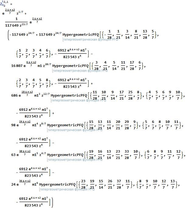
(4.11)