Band strutures of hybrid graphene quantum dots with magnetic flux

Abstract

We study the band structures of hybrid graphene quantum dots subject to a magnetic flux and electrostatic potential. The system is consisting of a circular single layer graphene surrounded by an infinite bilayer graphene. By solving the Dirac equation we obtain the solution of the energy spectrum in two regions. For the valley $K$, it is found that the magnetic flux strongly acts by decreasing the gap and shifting energy levels away from zero radius with some oscillations, which are note observed for null flux case. As for the valley $K^{\prime}$, the energy levels rapidly increase when the radius increases. A number of oscillations appeared that is strongly dependent on the values taken by the magnetic flux.

Hybrid graphene, quantum dots, magnetic flux, electrostatic potential.

1 Introduction

Quantum dots (QDs) in graphene are very small particles with unique electronic and optical properties [1, 2, 3, 4, 5, 6]. Since they are highly tunable, then they can serve as interesting building blocks for materials that might be used to advance a wide range of applications such as solar cells, medical imaging and quantum computing. Because of the Klein tunneling effect and the absence of the gap in the energy spectrum, Dirac fermions cannot be confined by electrostatic potentials [7]. One solution to overcome such situation is to realize QDs for instance using thin single-layer graphene (SLG) strips [8, 9] or nonuniform magnetic fields [10]. Generally, the electronic and optical properties of fermions in graphene depend on shapes and edges of QDS [11].

On the other hand, A-B bilayer graphene (BLG) consists of two SLG sheets where the A and B atoms in different layers are on top of each other [12], called also Bernal stacking. The most important interaction between the two layers is represented by a direct overlap integral between A and B atoms on top of each other. BLG presents some particularities for instance an external electric field, realized by external gate potentials, can induce a tunable band gap in its energy spectrum contrary to SLG.

Very recently a new generation of circular graphene QDs has been proposed based on a hybrid system [13]. Indeed, it was demonstrated that charge carriers can be confined in SLG and BLG islands in a hybrid QD-like structure made of SLG-BLG junctions. As a result, it is found that the energy levels exhibit characteristics of interface states in addition to the emergence of anti-crossings and closing of the band gap in the presence of a bias potential.

Motivated by the results reported in [13], we consider a geometry made of a circular SLG QD subjected to a magnetic flux and surrounded by an infinite BLG sheet as depicted in Fig. 1. We solve Dirac equation in both regions and determine in the first stage the eigenspinors. To derive equations governing the energy levels, we use the zigzag boundary conditions at interface. We numerically analyze our results and show that the magnetic flux differently acts on the energy levels for both valleys $K$ and $K^{\prime}$.

2 SLG quantum dots–BLG infinite

We consider a geometry made of a circular SLG QD of radius $r_{0}$ in the presence of a magnetic flux $\phi$ embedded in infinite BLG containing $A_{1}$, $B_{1}$ in first layer and $A_{2}$, $B_{2}$ in second one (Fig. 1).

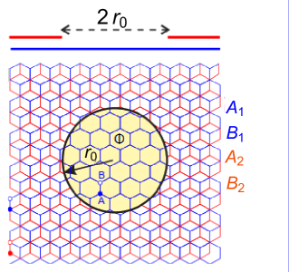
Figure 1: (color online) Circular SLG quantum dot in the presence of the magnetic flux $\Phi$ surrounded by an infinite BLGS.

The hybrid system can be described by the following Hamiltonian

$$H=v_{F}\ \vec{\sigma}\cdot(\vec{p}+e\vec{A})+U_{1}\mathbb{I}$$ (1)

where the vector potential associated to the magnetic flux $\Phi$ is given by

$$A(r)=\frac{h}{e}\frac{\Phi}{2\pi r}\hat{e_{\theta}}$$ (2)

and $\hat{e_{\theta}}$ is the unit vector for the azimuthal, $U_{1}$ is the potential applied to SLG, $\sigma_{i}$ are Pauli matrices. To do not couple the two valleys $K$ and $K^{\prime}$, we assume that the spatial extension of the flux line is large in comparison to the lattice constant.

2.1 Eigenspinors for the two valleys

To determine the eigenspinors of fermions in monolayer graphene subjected to magnetic flux, we consider the basis $\Psi^{\tau}(r,\theta)=(\Psi^{\tau}_{A},\Psi^{\tau}_{B})^{T}$ in polar coordinates $(r,\theta)$ because of the system symmetry. The valley index $\tau=+1$ refers to $K$ and $\tau=-1$ to $K^{{}^{\prime}}$. By showing that $[H,J_{z}]=0$, then the separability imposes such as

$$\Psi^{\tau}(r,\theta)=e^{im\theta}\begin{pmatrix}\chi^{\tau}_{A}(r)\\ ie^{-i\tau\theta}\chi^{\tau}_{B}(r)\end{pmatrix}$$ (3)

where $m=0,\pm 1,\pm 2,\cdots$ are eigenvalues of $L_{z}$ associated to the total angular momentum $J_{z}=L_{z}+\frac{\hbar}{2}\sigma_{z}$. To proceed further, let us write the Hamiltonian (1)

$$H=v_{F}\hbar\begin{pmatrix}u_{1}&\pi_{+}\\ \pi_{-}&u_{1}\end{pmatrix}$$ (4)

in terms of the operators

$$\pi_{\pm}=e^{\pm i\varphi}\left(-i\frac{\partial}{\partial\xi}\pm\frac{\tau}{\xi}\frac{\partial}{\partial\theta}\pm i\frac{\Phi}{\xi}\right)$$ (5)

such that the change of variable $\xi=\frac{r}{r_{0}}$ and the dimensionless quantities $\varepsilon=\frac{Er_{0}}{\hbar v_{F}}$, $u_{1}=\frac{U_{1}r_{0}}{\hbar v_{F}}$ are used.

The eigenvalue equation $H\Psi(\xi,\theta)=\varepsilon\Psi(\xi,\theta)$ allows to find two coupled equations

$$\left(\frac{\partial}{\partial\xi}-\frac{\tau m-1+\Phi}{\xi}\right)\chi^{\tau}_{B}=\left(\varepsilon-u_{1}\right)\chi^{\tau}_{A}$$ (6)

$$\left(\frac{\partial}{\partial\xi}+\frac{\tau m+\Phi}{\xi}\right)\chi^{\tau}_{A}=-\left(\varepsilon-u_{1}\right)\chi^{\tau}_{B}$$ (7)

By injecting (7) into (6) we obtain a second order differential equation for $\chi_{A}^{\tau}$

$$\left[\frac{\partial^{2}}{\partial\xi^{2}}+\frac{1}{\xi}\frac{\partial}{\partial\xi}-\frac{1}{\xi^{2}}\left(\tau m+\Phi\right)^{2}+\left(\varepsilon-u_{1}\right)^{2}\right]\chi^{\tau}_{A}=0$$ (8)

having the Bessel function as solution

$$\chi^{\tau}_{A}(\xi)=N^{\tau}J_{\nu}(\lambda\xi)$$ (9)

where we have set $\lambda=\varepsilon-u_{1}$ and a new quantum number $\nu=\tau m+\Phi$ depending on the valley index $\tau$ and flux $\Phi$, $N^{\tau}$ is a constant of normalization. Now replacing (9) in (7), we end up with the second component

$$\chi^{\tau}_{B}(\xi)=-\tau N^{\tau}J_{\nu-\tau}(\lambda\xi)$$ (10)

With the help of some relations between Bessel functions, we finally obtain the eigenspinors in monolayer graphene, which are

$$\Psi^{\tau}(\xi,\theta)=e^{im\theta}\begin{pmatrix}N^{\tau}J_{\nu}(\lambda\xi)\\ ie^{i\tau\theta}\tau N^{\tau}J_{\nu+\tau}(\lambda\xi)\end{pmatrix}$$ (11)

To achieve our task we consider the BLG region described by Hamiltonian for the valley $K$ $(\tau=+1)$

$$H^{+}=\begin{pmatrix}u_{+}+u_{-}&p_{+}&t^{{}^{\prime}}&0\\ p_{-}&u_{0}+\delta&0&0\\ t^{{}^{\prime}}&0&u_{0}-\delta&p_{-}\\ 0&0&p_{+}&u_{0}-\delta\end{pmatrix}$$ (12)

in the basis $(\Phi_{A_{1}}^{+},\Phi_{B_{1}}^{+},\Phi_{A_{2}}^{+},\Phi_{B_{2}}^{+})$ and we have set $p_{\pm}=p_{x}\pm ip_{y}$, $t^{{}^{\prime}}=\frac{tr_{0}}{\hbar v_{F}}$, $u_{+}=\frac{u_{1}+u_{2}}{2}$, $u_{-}=\frac{u_{1}-u_{2}}{2}$, and $u_{1,2}=\frac{U_{1,2}r_{0}}{\hbar v_{F}}$, with $U_{1,2}$ are the potentials at the two layers. In this region, the eigenspinors can be decoupled as

$$\Phi^{+}(\xi,\theta)=e^{im\theta}\begin{pmatrix}\chi^{+}_{A_{1}}(\xi)\\ ie^{-i\theta}\chi^{+}_{B_{1}}(\xi)\\ \chi^{+}_{B_{2}}(\xi)\\ ie^{i\theta}\chi^{+}_{A_{1}}(\xi)\end{pmatrix}$$ (13)

and then the eigenvalue equation gives rise to the set

$$\left(\frac{d}{d\xi}-\frac{m-1}{\xi}\right)\chi^{+}_{B_{1}}=\left(\varrho-u_{-}\right)\chi^{+}_{A_{1}}-t{{}^{\prime}}\chi^{+}_{B_{2}}$$ (14)

$$\left(\frac{d}{d\xi}+\frac{m}{\xi}\right)\chi^{+}_{A_{1}}=-\left(\varrho-u_{-}\right)\chi^{+}_{B_{1}}$$ (15)

$$\left(\frac{d}{d\xi}+\frac{m+1}{\xi}\right)\chi^{+}_{A_{2}}=\left(\varrho+u_{-}\right)\chi^{+}_{B_{2}}(\rho)-t{{}^{\prime}}\chi^{+}_{A_{1}}$$ (16)

$$\left(\frac{d}{d\xi}-\frac{m}{\xi}\right)\chi^{+}_{B_{2}}=-\left(\varrho+u_{-}\right)\chi^{+}_{A_{2}}$$ (17)

with $\varrho=\epsilon-u_{+}$. These equations can be decoupled to obtain for instance the following one for $\chi^{k}_{A_{1}}$

$$\left(\frac{d^{2}}{d\xi^{2}}+\frac{1}{\xi}\frac{d}{d\xi}-\frac{m^{2}}{\xi^{2}}-\mu^{2}_{\pm}\right)\chi^{+}_{A_{1}}=0$$ (18)

showing the eigenvalues

$$\mu_{\pm}=\left[-\left(\varrho^{2}+u_{-}^{2}\right)\pm\left[\left(\varrho^{2}-u_{-}^{2}\right)t^{{}^{\prime}2}+4\varrho^{2}u_{-}^{2}\right]^{\frac{1}{2}}\right]^{\frac{1}{2}}$$ (19)

and the appropriate solutions vanishing at $r\longrightarrow\infty$ is the modified Bessel function of the second kind $K_{m}^{\pm}=K_{m}(\mu_{\pm}\xi)$, then we have

$$\chi^{+}_{A_{1}}(\xi)=N^{+}_{1}K_{m}^{+}+N^{+}_{2}K_{m}^{-}$$ (20)

This can be used to derive the remaining components of the eigenspinors as follows

$$\chi^{+}_{B_{1}}=\frac{1}{\varrho-u_{-}}\left[N_{1}^{+}\mu_{+}K_{m-1}^{+}+N_{2}^{+}\mu_{-}K_{m-1}^{-}\right]$$ (21)

$$\chi^{+}_{B_{2}}=\frac{1}{(\varrho-u_{-})t^{{}^{\prime}}}\left[N_{1}^{+}\eta_{+}K_{m}^{+}+N_{2}^{+}\eta_{-}K_{m}^{-}\right]$$ (22)

$$\chi^{+}_{A_{2}}=\frac{1}{(\varrho^{2}-u_{-}^{2})t^{{}^{\prime}}}\left[N_{1}^{+}\mu_{+}\eta_{+}K_{m+1}^{+}+N_{2}^{+}\mu_{-}\eta_{-}K_{m+1}^{-}\right]$$ (23)

where we have defined

$$\eta_{\pm}=(\varrho-u_{-})^{2}+\mu_{\pm}^{2}$$ (24)

$N^{+}_{1}$ and $N^{+}_{2}$ are two constants of normalization. It is showed that (19) possess a gap in the energy spectrum [14]

$$\Delta=\frac{\Delta U}{\sqrt{1+\frac{\Delta U^{2}}{t^{2}}}}$$ (25)

resulted from the Mexican-hat shaped low-energy dispersion in pristine BLG. In the limit $\Delta U\ll t$ it behaves as potential scale, i.e. $\Delta\approx{\Delta U}$.

As concerning the valley $K^{\prime}$, one can easy show that the radial parts of the corresponding eigenspinors can be linked to those for the valley $K$. Indeed, solving the eigenvalue equation with the basis

$$\Phi^{-}(\xi,\theta)=e^{im\xi}\begin{pmatrix}\chi^{-}_{A_{1}}(\xi)\\ ie^{i\theta}\chi^{-}_{B_{1}}(\xi)\\ \chi^{K^{{}^{\prime}}}_{B_{2}}(\xi)\\ ie^{-i\theta}\chi^{-}_{A_{2}}(\xi)\end{pmatrix}$$ (26)

to end up with the relations

$$\chi^{-}_{A_{1}}(\xi)=\chi^{+}_{B_{2}}(\xi)$$ (27)

$$\chi^{-}_{B_{1}}(\xi)=\chi^{+}_{A_{2}}(\xi)$$ (28)

$$\chi^{-}_{B_{2}}(\xi)=\chi^{+}_{A_{1}}(\xi)$$ (29)

$$\chi^{-}_{B_{1}}(\xi)=\chi^{+}_{B_{1}}(\xi)$$ (30)

In the next we will see how the above results will be used to analyze the influence of the applied magnetic flux on the energy levels.

2.2 Zigzag boundary conditions

To derive equations describing the energy levels for the two valleys, we use the zigzag boundary conditions [15]. Then, at the interface $\xi=1$, namely $r=r_{0}$, between SLG and BLG we have the continuities

$$\Psi^{\tau}_{A}(1,\theta)=\Phi_{A_{1}}^{\tau}(1,\theta)$$ (31)

$$\Psi^{\tau}_{B}(1,\theta)=\Phi_{B_{1}}^{\tau}(1,\theta)$$ (32)

$$0=\Phi_{A_{2}}^{\tau}(1,\theta)$$ (33)

Consequently, (31-33) give

$$M^{+}\begin{pmatrix}N^{+}\\ N^{+}_{1}\\ N^{+}_{2}\end{pmatrix}=0$$ (34)

for the valley $K$ ($\tau=+1$) such that the matrix is

$$M^{+}=\begin{pmatrix}-J_{\nu}(\lambda)&K_{m}^{+}&K_{m}^{-}\\ J_{\nu-1}(\lambda)&a_{+}K_{m-1}^{+}&a_{-}K_{m-1}^{-}\\ 0&b_{+}K_{m}^{+}&b_{-}K_{m}^{-}\end{pmatrix}$$ (35)

where we have set

$$a_{\pm}=\frac{\mu_{\pm}}{\varrho-u_{-}},\qquad b_{\pm}=\frac{\left(\varrho-u_{-}\right)^{2}+\mu_{\pm}^{2}}{\left(\varrho-u_{-}\right)t{{}^{\prime}}}$$ (36)

Regarding $K^{{}^{\prime}}$, we fix $\tau=-1$ and use the corresponding eigenspinors to end up with

$$M^{-}\begin{pmatrix}N^{-}\\ N^{-}_{1}\\ N^{-}_{2}\end{pmatrix}=0$$ (37)

and the matrix reads as

$$M^{-}=\begin{pmatrix}-J_{\nu}(\lambda)&b_{+}K_{m}^{+}&b_{-}K_{m}^{-}\\ -J_{\nu+1}(a)&c_{+}K_{m-1}^{+}&c_{-}K_{m-1}^{-}\\ 0&K_{m}^{+}&K_{m}^{-}\end{pmatrix}$$ (38)

with the parameters

$$c_{\pm}=\frac{b_{\pm}\mu_{\pm}}{\varrho+u_{-}}$$ (39)

$N^{-}_{1}$ and $N^{-}_{2}$ are two constants of normalization. At this level we point out that the energy levels for both valleys are solutions of the two determinants

$$\det M^{+}=0,\qquad\det M^{-}=0$$ (40)

It is clear that form the complexity of the special functions involved in the eigenspinors, it is not easy to analytically derive an explicit expression of the energy levels. Then, to investigate the basic features of our hybrid system we will proceed numerically.

3 Numerical Analysis

We plot the energy levels $E$(eV) versus the dot radius $r_{0}$(nm) for the valleys $K$ and $K^{{}^{\prime}}$ under suitable conditions of the physical parameters. It is convenient for our task to choose the angular momenta $m=0,\pm 1,\pm 2,\pm 3$, magnetic flux $\Phi=\pm\frac{1}{2},\pm\frac{3}{2},\pm\frac{5}{2}$ and the biased potential $U_{1}=-U_{2}=0.1$ eV. We emphasis that the solid black horizontal lines in all figures show the band gap.

3.1 Valley $K$

As a first result regarding the valley $K$, we observe that the symmetry $E^{+}(m)=E^{+}(-m)$ is always preserved for all values taken by the magnetic flux.

Figure 2: (color online) Energy levels of the valley $K$ as a function of the dot radius $r_{0}$ for $m=0,\pm 1,\pm 2,\pm 3$ in the presence of the biased potential $U_{1}=-U_{2}=0.1$ eV and the magnetic flux $\Phi$ (a): $\frac{1}{2}$, (b): $-\frac{1}{2}$.

Fig. 2a presents the behavior of the energy levels $E$ for the value $\Phi=\frac{1}{2}$. We notice that the energy levels are shifted and band gap decreased compared to the non-flux case [13]. As long as the radius increases we see that $E$ increase but gap continue decreasing. We observe another behavior in Fig. 2b with $\Phi=-\frac{1}{2}$. Indeed, the energy levels show a maximum corresponds to $m=0$ and $r_{0}=0$, after they oscillate to reach a minimum at $r_{0}=4.8$ nm and then increase.

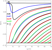
Figure 3: (color online) The same as in Fig. 2, but now with the magnetic flux $\Phi$ (a): $\frac{3}{2}$, (b): $-\frac{3}{2}$.

Now we increase the magnetic flux and choose $\Phi=\frac{3}{2}$ as presented in Fig. 3b. In the present case, the shift of the energy levels becomes clear and the decrease in gap as well. Remarkably for the negative value $\Phi=-\frac{3}{2}$ in Fig. 3b we notice that the values $m=\pm 1$ show a similar behavior as in Fig. 2b for $m=0$ but with less oscillation. In addition, we observe here that $m=0$ and $m=\pm 1$ correspond to the minima $r_{0}=12.67$ nm and $r_{0}=10.11$ nm, respectively.

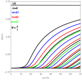
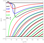
Figure 4: (color online) The same as in Fig. 2, but now the magnetic flux $\Phi$ (a): $\frac{5}{2}$, (b): $-\frac{5}{2}$.

By increasing the magnetic flux to $\phi=\frac{5}{2}$ in Fig. 4a, we notice that the shift and gap become more important. As for $\phi=-\frac{5}{2}$ in Fig. 4b, we observe that the number of oscillations increases to three corresponding to the quantum numbers $m=0$, $m=\pm 1$ and $m=\pm 2$ with the minima $r_{0}=18.81$ nm, $r_{0}=15.69$ nm and $r_{0}=13.67$ nm, respectively.

3.2 Valley $K^{\prime}$

As for the valley $K^{\prime}$, the energy levels show different behavior resulted form the choice of the magnetic flux compared to the valley $K$. Indeed, the first difference that should be noticed we do not have the symmetry $E^{-}(m)\neq E^{-}(-m)$ with $m=0,1,2,3$ correspond to solid lines and the negative numbers to dashed lines in plots below. In addition, for $\Phi=\frac{1}{2}$ in Fig. 5a, the energy levels rapidly increase and the particularity is seen for $m=-1$ where the level overcomes that for $m=1$. The situation is completely changed for $\Phi=-\frac{1}{2}$ in Fig. 5b because we observe that the level $m=-1$ is under $m=1$.

   

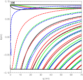
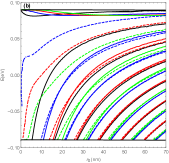
Figure 5: (color online) Energy levels of the valley $K^{\prime}$ as a function of the dot radius $r_{0}$ for $m=0,\pm 1,\pm 2,\pm 3$ in the presence of the biased potential $U_{1}=-U_{2}=0.1$ eV and the magnetic flux $\Phi$ (a): $\frac{1}{2}$, (b): $-\frac{1}{2}$.

The behavior of the energy levels becomes more clear in Fig. 6a with $\Phi=\frac{3}{2}$ compared to Fig. 5a. Now as concerning the negative value $\Phi=-\frac{3}{2}$, Fig. 6b shows a mixing of the energy levels and we observe that some oscillations with different amplitudes start to take place. These are corresponding to the quantum numbers $m=0$ (black solid line), $m=-1$ (blue dashed line), $m=-2$ (red dashed line), $m=-3$ (green dashed line).

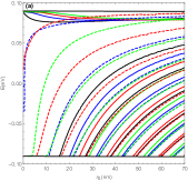
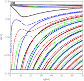
Figure 6: (color online) The same as in Fig. 5, but now with the magnetic flux $\Phi$ (a): $\frac{3}{2}$, (b): $-\frac{3}{2}$.

We now consider $\Phi=\frac{5}{2}$ in Fig. 7a and observe an important change in the energy levels such that shifts increase. In Fig. 7b with $\Phi=-\frac{5}{2}$, we notice that the number of oscillations increase as well. These results show the manifestation of the magnetic flux and its impact on the energy levels.

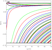
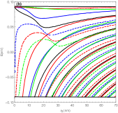
Figure 7: (color online) The same as in Fig. 5, but now with the magnetic flux $\Phi$ (a): $\frac{5}{2}$, (b): $-\frac{5}{2}$.

4 Conclusion

We have studied the influence of a magnetic flux on the energy levels of a hybrid graphene. More precisely, we have considered a graphene quantum dot surrounded by a infinite bilayer graphene. Our result showed that the energy levels can oscillate, increase and shift under appropriate choice of flux and variation of the dot radius. We have found that the energy levels of the valleys $K$ and $K^{\prime}$ present different behaviors.

References

- [1] A. V. Rozhkov, G. Giavaras, Y. P. Bliokh, V. Freilikher, and F. Nori, Phys. Rep. 503, 77 (2011).
- [2] Z. Z. Zhang, K. Chang, and F. M. Peeters, Phys. Rev. B 77, 235411 (2008).
- [3] D. Bischoff, A. Varlet, P. Simonet, M. Eich, H. C. Overweg, T. Ihn, and K. Ensslin, Appl. Phys. Rev. 2, 031301 (2015).
- [4] B. Trauzettel, D. V. Bulaev, D. Loss, and G. Burkard, Nat. Phys. 3, 192 (2007).
- [5] J. M. Pereira Jr, F. M. Peeters, P. Vasilopoulos, R. N. Costa Filho, and G. A. Farias, Phys. Rev. B 79, 195403 (2009).
- [6] P. Recher and B. Trauzettel, Nanotechnol. 21, 302001 (2010).
- [7] M. I. Katsnelson, K. S. Novoselov, and A. K. Geim, Nat. Phys. 2, 620 (2006).
- [8] N. M. R. Peres, A. H. Castro Neto, and F. Guinea, Phys. Rev. B 73, 241403 (2006).
- [9] P. G. Silvestrov and K. B. Efetov , Phys. Rev. Lett. 98, 016802 (2007).
- [10] C. Berger et al., Science 312, 1191 (2006).
- [11] Alev Devrim Güçlü, Pawel Potasz, Marek Korkusinski, and Pawel Hawrylak, Graphene Quantum Dots (Springer Berlin Heidelberg, 2014).
- [12] E. McCann, D. S. L. Abergel, and V. I. Falko, Eur. Phys. J. Spec. Top. 148, 91 (2007).
- [13] M. Mirzakhani, M. Zarenia, S. A. Ketabi, D. R. da Costa, and F. M. Peeters, Phys. Rev. B 93, 165410 (2016).
- [14] E. McCann, D. S. L. Abergel, and V. I. Falko, Eur. Phys. J. Spec. Top. 148, 91 (2007).
- [15] M. Koshino, T. Nakanishi, and T. Ando, Phys. Rev. B 82, 205436 (2010).