Iterative, Deep, and Unsupervised
Synthetic Aperture Sonar Image Segmentation

Abstract

Deep learning has not been routinely employed for semantic segmentation of seabed environment for synthetic aperture sonar (SAS) imagery due to the implicit need of abundant training data such methods necessitate. Abundant training data, specifically pixel-level labels for all images, is usually not available for SAS imagery due to the complex logistics (e.g., diver survey, chase boat, precision position information) needed for obtaining accurate ground-truth. Many hand-crafted feature based algorithms have been proposed to segment SAS in an unsupervised fashion. However, there is still room for improvement as the feature extraction step of these methods is fixed. In this work, we present a new iterative unsupervised algorithm for learning deep features for SAS image segmentation. Our proposed algorithm alternates between clustering superpixels and updating the parameters of a convolutional neural network (CNN) so that the feature extraction for image segmentation can be optimized. We demonstrate the efficacy of our method on a realistic benchmark dataset. Our results show that the performance of our proposed method is considerably better than current state-of-the-art methods in SAS image segmentation.

I Introduction

Recently, deep learning frameworks applied for image segmentation have shown promising results [1, 2]. To segment distinct seabed textures in sonar images, a naive intuition is that we can use a similar network structure for seabed segmentation of SAS images because they have largely composted low-level textures. However, training a convolutional neural network (CNN) requires a considerable amount of labeled data to obtain good results. For SAS image segmentation, this means acquiring pixel-level annotations which is a costly process, and rarely do we have complete ground-truth from a diver survey. Consequently, humans often label regions which are easily recognized while forgoing areas difficult to distinguish such as region boundaries or blended regions. As a result, few pixel-level labeled datasets are available for training.

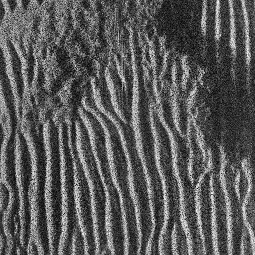
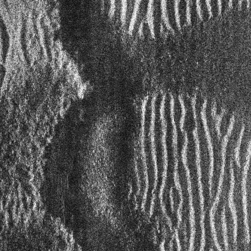
Figure 1: Sample SAS images containing various seabed types including large sand ripples and flat sandy seafloor.

Unsupervised image classification [3] has shown that embedding deep learning steps into a clustering algorithm is a promising direction. The essence of image-level clustering is to see every image as a region that only contains one high-level semantic texture, but the regions’ boundaries are inaccurate. We apply this idea to the image segmentation task. Although we are going to do pixel-level segmentation, from our observations regions containing a single texture will produce similar pixel predictions. If we can find accurate boundaries to differentiate the regions containing a single texture, then the image segmentation process can be transferred into the region-level classification problem.

We devise a novel unsupervised segmentation method that combines deep learning and an iterative clustering technique producing an algorithm suitable for unsupervised seabed segmentation of SAS images. The basic idea is to use superpixels generated by CNN pseudo-labels to split one sonar image into many small regions. Each region is quantized into one superpixel feature that is the average softmax value and then a clustering process is performed to group these regions. Finally, we utilize the clustering results to update the CNN parameters to encourage more accurate predictions of a segmentation network.

We evaluate our method, which we call iterative deep unsupervised segmentation (IDUS), against several comparison methods on a contemporary real-world SAS dataset. We show compelling performance of IDUS against existing state-of-the-art methods for SAS image co-segmentation. Additionally, we show an extension of our method which can obtain even better results when semi-labeled data is present. Specifically, our work makes two main contributions:

1. We devise a new iterative method to integrate the merits of best-known unsupervised superpixel segmentation along with a deep feature extractor.

2. Our approach does not depend on any specific network structure or superpixel generation algorithm. The user can adjust the algorithm easily according to different segmentation tasks.

II Technical Approach

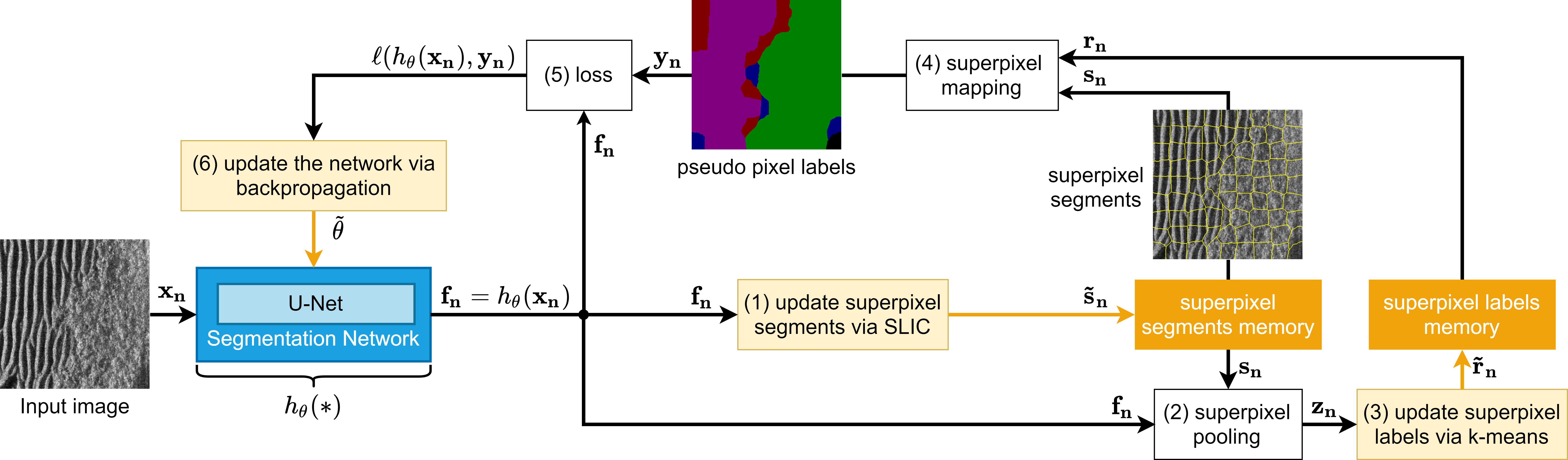
Figure 2: An iteration of IDUS: (1) Use SLIC [4] to generate the new superpixel segments. (2) Quantize pixel features into superpixel features. (3) Cluster superpixel features by k-means to update the class assignments in memory. (4) Map superpixel labels to pseudo pixel labels. (5) Compute the loss via the pseudo pixel labels and the network softmax outputs. (6) Update the network via backpropagation.

A recent method called DeepCluster [3] demonstrates that the combination of clustering techniques and CNNs show promise in unsupervised learning of deep features on image classification dataset is possible. The benefit of DeepCluster is that the training method is more generally and easily transferred to other tasks. This benefit motivates us to develop our own work on unsupervised image segmentation because the method not only will not be limited to the sonar images, but it can also be used in other segmentation tasks.

Notation. Given a set $\mathbf{X}=\left\{\mathbf{x_{1}},...,\mathbf{x_{N}}\right\}$ of $N$ SAS images, $s_{n}^{k}$ is the $k$-th superpixel of the $n$-th image and $r_{n}^{k}$ are the pseudo-label of this superpixel. We use $h_{\theta}(\cdot)$ to denote the softmax output of a segmentation network (i.e. deep network), where $\theta$ is the parameters we need to optimize. The output has same size with the input image. Given an input image $\mathbf{x_{n}}$, the network maps the image into a feature map $\mathbf{f_{n}}=h_{\theta}(\mathbf{x_{n}})$ in which $f_{n}^{i}$ represent the feature of $i$-th pixel $x_{n}^{i}$ in this image.

Superpixel Pooling. To quantize the pixel-level features into region-level features $\mathbf{z_{n}}=Q_{pool}(\mathbf{x_{n}},\mathbf{f_{n}},\mathbf{s_{n}})$, we compute the feature’s mean from all the pixels making up the superpixel $z_{n}^{k}$ by the following equation:

$$z_{n}^{k}=\frac{1}{D}\sum_{i=1}^{D}f_{n}^{i}I(x_{n}^{i}\in s_{n}^{k}),$$ (1)

where $D$ denotes the number of pixels in the input image. $I(x_{n}^{i}\in s_{k}^{i})$ is an indicator function that is 1 if $x_{n}^{i}$ belongs to the superpixel $s_{n}^{k}$. The superpixel quantization makes sure that we can collect regional features of sufficient accuracy for the later clustering use.

Superpixel Mapping. Suppose we have already known a superpixel label $r_{n}^{k}$, then every pixel label $y_{n}^{i}$ in this superpixel should be the same. We use the following formula to describe this mapping:

$$y_{n}^{i}=\sum_{k=1}^{K_{n}}r_{n}^{k}I(x_{n}^{i}\in s_{n}^{k})$$ (2)

where $K_{n}$ denotes the number of superpixels in $n$th image. We use $\mathbf{y_{n}}=Q_{map}(\mathbf{x_{n}},\mathbf{r_{n}},\mathbf{s_{n}})$ to denote this process which we call superpixel mapping. It eliminates some classification errors and produces more robust class assignments for pixels.

The Simplest Version of IDUS. Figure 2 shows an iteration of the simplest version of IDUS after initialization. Here, we assume that the minibatch only contains one image. The superpixel segments memory stores the boundary of every superpixel and the superpixel labels memory stores the superpixel labels. We see the softmax vectors of network outputs as a kind of feature representation, due to it has the same size of the inputs and contains the distance information between a region texture and cluster centroids. In an iteration, we first use superpixel segments to quantize the pixel features into superpixel features (Eq. (1)) and use $k$-means to update the superpixel labels. Next, we map the superpixel labels to pixel labels (Eq. (2)) and use the pseudo-class assignments to update the network via back-propagation. As shown in Figure 2, IDUS alternates between generating pseudo ground-truth labels and updating the network parameters.

The Complete Version of IDUS Given a set of training images $\mathbf{X_{T}}=\left\{\mathbf{x_{n}}\right\}_{n=1}^{N_{T}}$, we update the model’s parameters $\theta$ by solving the following problem,

$$\min_{\theta}\frac{1}{N_{T}}\sum_{n=1}^{N_{T}}\ell(h_{\theta}(\mathbf{x_{n}}),Q_{map}(\mathbf{x_{n}},\mathbf{r_{n}},\mathbf{s_{n}})),$$ (3)

where $\ell$ is a loss function and $\mathbf{r_{n}}$, $\mathbf{s_{n}}$ will be initialized before performing the algorithm. After training the model for $U_{E}$ epochs, we extract the feature maps $\left\{\mathbf{f_{n}}\right\}_{n=1}^{N_{T}}$ of all training images based on the current model’s parameters $\theta_{i}$ where $i$ is the number of iteration. Then, we pool the feature maps to regional features $\left\{\mathbf{z_{n}}\right\}_{n=1}^{N_{T}}$ and cluster them into $M$ groups based on the optimization goal

$$\min_{C\in\mathbb{R}^{M\times d}}\sum_{m=1}^{M}\sum_{n=1}^{N}\sum_{k=1}^{K_{n}}\min_{r_{n}^{k}\in[1,M]}\|z_{n}^{k}-c_{m}\|I(r_{n}^{k}==m),$$ (4)

where $c_{m}$ is the centroid feature of class $m$ and $d$ is the length of feature dimension. With this clustering criterion, the regional features will be clustered and used to produced new labels $\left\{\mathbf{r_{n}}\right\}_{n=1}^{N_{T}}$; and then, they will be assigned to the corresponding superpixels.

The overall idea of IDUS can be summarized in Algorithm 1. We update the superpixel boundaries every $U_{S}$ epochs and the algorithm terminates after a fixed number of iterations.

Algorithm 1 Iterative Deep Unsupervised Segmentation

1:  Initialize superpixel segments, labels $\left\{\mathbf{s_{n}},\mathbf{r_{n}}\right\}_{n=1}^{N_{T}}$ of $N_{T}$ training images. And map the regional labels to pseudo pixel labels $\left\{\mathbf{y_{n}}\right\}_{n=1}^{N_{T}}$ by Eq 2.

2:  Assign intervals $U_{E}$, $U_{S}$ for updating the pseudo-ground-truth and superpixel boundaries.

3:  repeat

4:     Given training data set $\left\{\mathbf{x_{n}},\mathbf{y_{n}}\right\}_{n=1}^{N_{T}}$, update the model’s parameters $\theta$ based on the problem Eq (3).

5:     if every $U_{S}$ epochs then

6:        Update superpixel boundaries $\left\{\mathbf{s_{n}}\right\}_{n=1}^{N}$ based on the model of current iteration.

7:     end if

8:     if every $U_{E}$ epochs then

9:        Use the model parameters of current iteration $\theta_{i}$ to generate pixel-level features $\{\mathbf{f_{n}}\}_{n=1}^{N_{T}}$.

10:        Pool the pixel-level features into regional features by Eq (1).

11:        Cluster the regional features based on criterion Eq (4) and reassign new pseudo labels $\left\{\mathbf{r_{n}}\right\}_{n=1}^{N_{T}}$ to each superpixel.

12:     end if

13:  until reach the maximum iteration.

14:  Output the model’s parameters $\theta$.

Layer Name	Layer Function	Dim.	# Filters	Input
up1	Upsampling	2$\times$2	N/A	res4
merge1	Concatenate	N/A	N/A	up1, res3
conv1a	Conv+BN+ReLU	3$\times$3	256	merge1
conv1b	Conv+BN+ReLU	3$\times$3	256	conv1a
up2	Upsampling	2$\times$2	N/A	conv1b
merge2	Concatenate	N/A	N/A	up2, res2
conv2a	Conv+BN+ReLU	3$\times$3	128	merge2
conv2b	Conv+BN+ReLU	3$\times$3	128	conv2a
up3	Upsampling	2$\times$2	N/A	conv2b
merge3	Concatenate	N/A	N/A	up3, res1
conv3a	Conv+BN+ReLU	3$\times$3	64	merge3
conv3b	Conv+BN+ReLU	3$\times$3	64	conv3a
up4	Upsampling	2$\times$2	N/A	conv3b
merge4	Concatenate	N/A	N/A	up4, res_conv
conv4a	Conv+BN+ReLU	3$\times$3	32	merge4
conv4b	Conv+BN+ReLU	3$\times$3	32	conv4a
up5	Upsampling	2$\times$2	N/A	conv4b
conv5a	Conv+BN+ReLU	3$\times$3	16	up5
conv5b	Conv+BN+ReLU	3$\times$3	16	conv5a
seg_head	Conv+Softmax	3$\times$3	7	conv5b

TABLE I: Description of decoder and segmentation head of the U-Net used in IDUS. This decoder is preceded by a pre-trained ResNet-18 network. “Conv+BN+ReLU” is 2D convolutional followed by Batch Normalization followed by rectified linear unit (ReLU) activation and “Softmax” denotes the softmax function. We use layers res_conv, res1, res2, res3, and res4 to denote the output of ResNet-18’s first convolutional layer and building blocks, respectively. Layer conv5b is the decoder output and layer seg_head is the segmentation head output.

Implementation Details The backbone model used by IDUS is U-Net[2] equipped with ResNet-18 encoder that pre-trained on ImageNet [5]. TABLE I shows the decoder and segmentation head (pixel-level linear classifier) of U-Net. For the initialization, we first concatenate the feature maps of the output of the first and third convolutional blocks in ResNet-18 of every image; and then, we use the idea of texton [6] to initialize the pseudo labels and a two-step texton selection [7] to reduce the computation time. We train the IDUS with mini-batch size fifteen on an NVIDIA Titan X GPU (12GB) with the PyTorch package [8]. The loss function we use is the mean of dice loss [9] and cross-entropy loss. We use weights $w_{m}^{ept}=1/r_{m}$ and $w_{m}^{dice}=1/\sqrt{r_{m}}$, where $r_{m}$ was the proportion of $m$th class label in training samples, to balance the class weights of two losses, respectively. Batch normalization layers [10] are added after each convolutional layer (except the segmentation head) to accelerate the loss convergence. The model’s parameters are initialed by a uniform distribution following the scaling of [11] and optimized by Adam [12] algorithm with weight decay value $10^{-9}$. In every iteration, the learning rate of the model is initialized at $10^{-4}$ and decreased by $0.1$ every fifty epochs. The updating interval of superpixel labels and boundaries is 200 and we do this five times throughout training. Consequently, we train for 1000 epochs where every 200 epochs we update the superpixel labels and boundaries.

III Experimental Results

III-A Experimental Setup

The dataset we use to test the performance of IDUS is composed of 113 images collected from a high-frequency SAS system which are semi-labeled (i.e. not every pixel is labeled in every image). The images contain seven distinct labeled seabed areas: shadow (SH), dark sand (DS), bright sand (BS), seagrass (SG), large sand ripple (SR), rock (RK), and small sand ripple (SR). The images were originally $1001\times 1001$ pixels in size which we downsample to $512\times 512$ pixels for computational efficiency.

Comparison Methods. To show the effectiveness of our method, we compare with two recent methods [13, 14] used in SAS seabed environment image segmentation. Following, we give the implementation details we use in generating the comparison methods as no source code is publicly available to evaluate. We make a best effort attempt to reproduce the methods as given in their respective sources.

Lianantonakis, et al. (2007) [13]. This method uses Haralick features [15] derived from the gray-level co-occurrence matrix (GLCM) and couples this with active contours to arrive at a binary class mapping. We extend this work to multiple classes by simply using the same feature descriptors as the original work but apply $k$-means++ to cluster; a similar replication approach is used in [16]. We ran $k$-means++ with 100 random initializations and selected the run that produces the minimum within cluster sum of squares error in a manner consistent with [17].

Zare, et al. (2017) [14]. In this work, the feature sets are produced by Sobel edge descriptors (Sobel) [18], histograms of oriented gradients (HOG) [19], and local binary pattern (LBP) features [20]. For each feature descriptor, we use the same sliding window strategy of Lianantonakis, et al.[13] to derive a feature vector for each pixel.

For the comparison methods, the co-segmentation strategy contains four main steps:

1. Feature extraction to extract a set of feature maps from the input sonar images.

2. Performing SLIC [4] on the extracted features to generate superpixel features by Eq (1).

3. Unsupervise cluster all the superpixels and provide each superpixel a cluster assignment.

4. Pixels inside a superpixel are assigned the same cluster by Eq (2) to get pixel-level co-segmentation.

For the co-segmentation strategy of IDUS, we train a segmentation network by IDUS on the entire dataset first, and then directly use the network outputs computed from the input sonar images as the final co-segmentation results.

III-B Results

(a) Lianantonakis, et al. (2007) [17] 2009

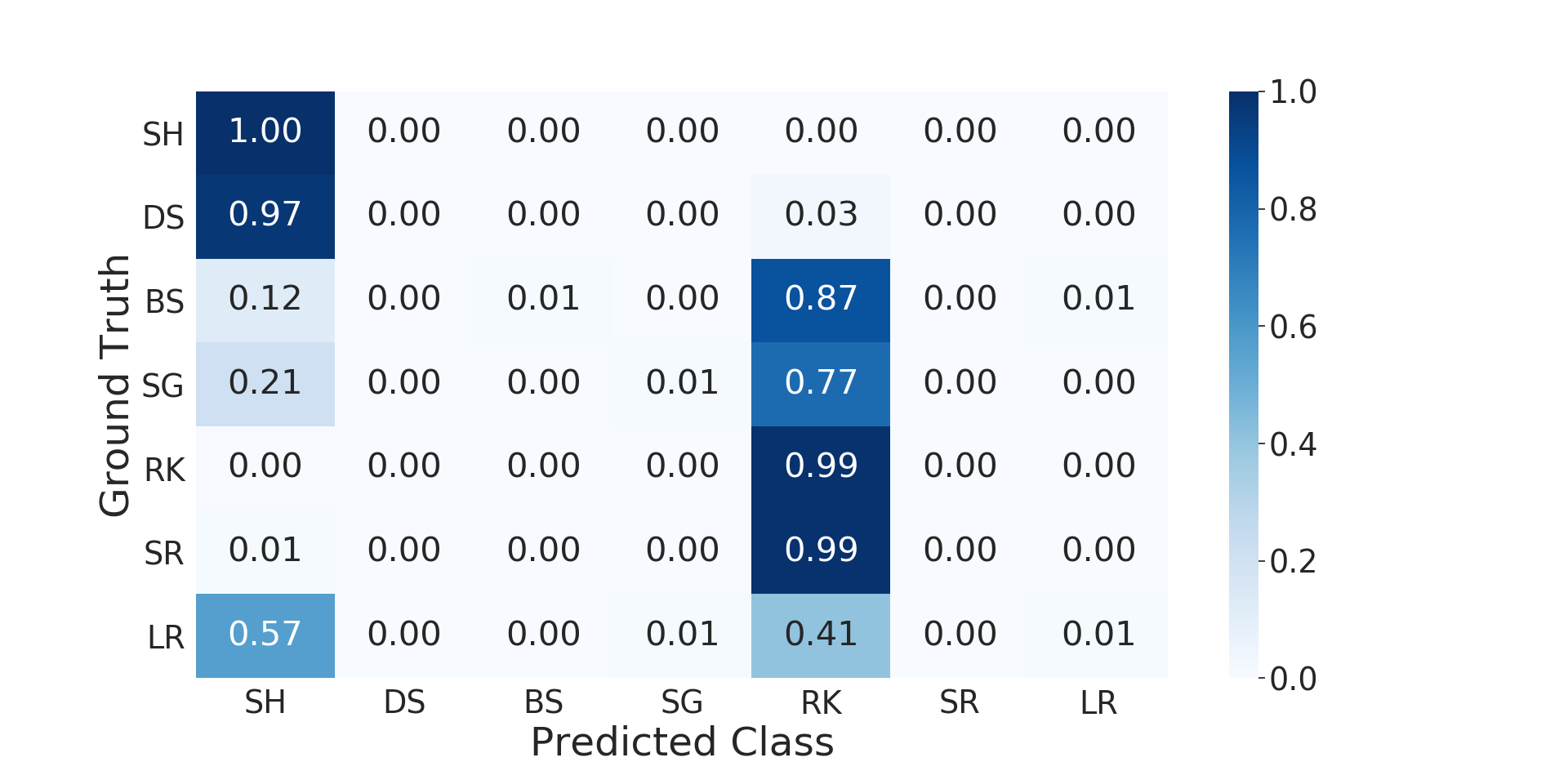
(b) Zare, et al. (2017) [14] 2017

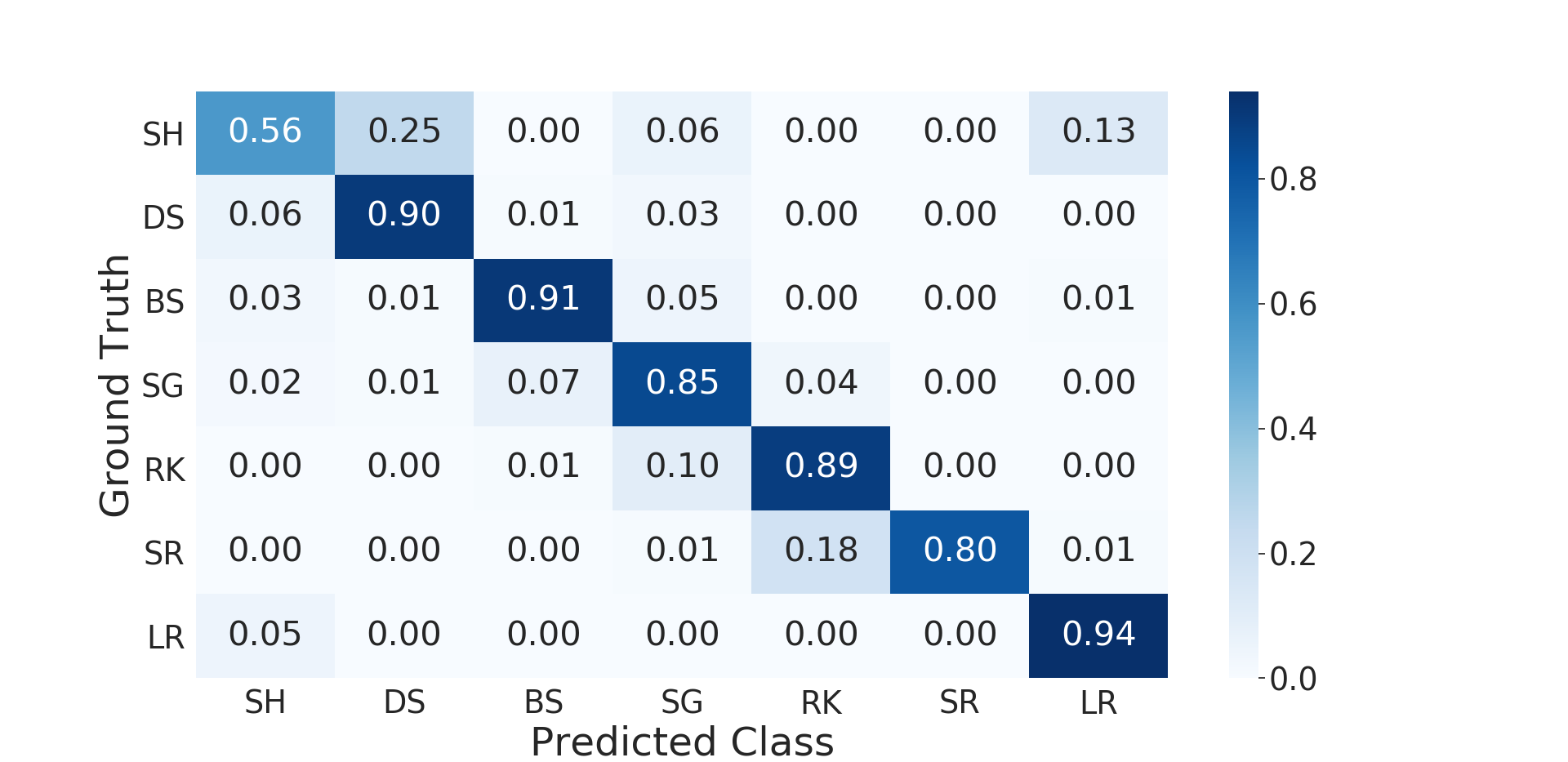
(c) IDUS

Figure 3: Confusion matrices of IDUS along with comparisons in the first experiment. Higher values along the diagonal indicate better performance.

We use the confusion matrix as a criterion to evaluate the co-segmentation performance of IDUS and the comparison methods on the entire dataset (113 images). A confusion matrix shows the proportion of an assigned class predicted by the algorithm for a given ground-truth class. Ideally, the ground-truth class and the predicted class overlap entirely giving a proportion of one. However, in practice, the predicted class by co-segmentation usually do not perfectly match with the ground-truth class resulting in a proportion less than one.

As a result of performing unsupervised segmentation, class assignments by the algorithm must be mapped to ground-truth classes. We perform this assignment by initially using a random disjoint assignment among the possible classes and then compute the confusion matrix. Next, we re-sort the columns of the matrix in such a way so that the sum of diagonal elements in the new confusion matrix is maximized. For the co-segmentation of the comparison methods, we set the clusters number is the same as the number of ground-truth classes (seven class). For IDUS, we set the dimension of the network softmax output as seven. Therefore, we use a confusion matrix with size $7\times 7$ as the criterion for evaluating different methods.

Figure 3 shows the confusion matrices of IDUS and the comparison methods. As shown in the figure, IDUS results in superior co-segmentation results (Figure 3c) over the comparison methods (Figure 3a and b). Upon examining the confusion matrices, we notice some comparison methods do not provide enough discrimination ability to differentiate certain classes well. For example, Shadow (SH) and Dark Sand (DS) are clustered into the same class in Lianantonakis, et al. [13] (Figure 3a). However, such misclassification problems are diminished by IDUS (Figure 3c).

IV Conclusion

We propose an unsupervised method for SAS seabed image segmentation which works by iteratively clustering on superpixels while training a deep model. Our proposed method (iterative, deep, and unsupervised segmentation (IDUS)) does not require large amounts of labeled training data which are difficult to obtain for SAS. We show that IDUS obtains state-of-the-art performance on a real-world SAS dataset and show performance benefits by comparing against existing methods.

In future work, we will extend IDUS to combine with supervised or semi-supervised training data.

V Acknowledgements

This work was supported by the Office of Naval Research via grant N00014-19-1-2513. The authors thank the Naval Surface Warfare Center - Panama City Division for providing the data used in this work.

References

- [1] P. Liskowski and K. Krawiec, “Segmenting retinal blood vessels with deep neural networks,” IEEE TMI, vol. 35, no. 11, pp. 2369–2380, 2016.
- [2] O. Ronneberger, P. Fischer, and T. Brox, “U-net: Convolutional networks for biomedical image segmentation,” in MICCAI, 2015, pp. 234–241.
- [3] M. Caron, P. Bojanowski, A. Joulin, and M. Douze, “Deep clustering for unsupervised learning of visual features,” in Proceedings of the European Conference on Computer Vision (ECCV), 2018, pp. 132–149.
- [4] R. Achanta, A. Shaji, K. Smith, A. Lucchi, P. Fua, and S. Susstrunk, “SLIC superpixels compared to state-of-the-art superpixel methods,” IEEE Trans. Pattern Anal. Mach. Intell., vol. 34, no. 11, p. 2274–2282, Nov. 2012.
- [5] J. Deng, W. Dong, R. Socher, L.-J. Li, K. Li, and L. Fei-Fei, “ImageNet: A Large-Scale Hierarchical Image Database,” in CVPR09, 2009.
- [6] J. Malik, S. Belongie, T. Leung, and J. Shi, “Contour and texture analysis for image segmentation,” International Journal of Computer Vision, vol. 43, no. 1, pp. 7–27, 2001.
- [7] J. T. Cobb and A. Zare, “Multi-image texton selection for sonar image seabed co-segmentation,” in Defense, Security, and Sensing, 2013.
- [8] A. Paszke, S. Gross, F. Massa, A. Lerer, J. Bradbury, G. Chanan, T. Killeen, Z. Lin, N. Gimelshein, L. Antiga, A. Desmaison, A. Kopf, E. Yang, Z. DeVito, M. Raison, A. Tejani, S. Chilamkurthy, B. Steiner, L. Fang, J. Bai, and S. Chintala, “Pytorch: An imperative style, high-performance deep learning library,” in Advances in Neural Information Processing Systems, vol. 32, 2019.
- [9] C. H. Sudre, W. Li, T. Vercauteren, S. Ourselin, and M. J. Cardoso, “Generalised dice overlap as a deep learning loss function for highly unbalanced segmentations,” in Deep Learning in Medical Image Analysis and Multimodal Learning for Clinical Decision Support. Springer, 2017, pp. 240–248.
- [10] S. Ioffe and C. Szegedy, “Batch normalization: Accelerating deep network training by reducing internal covariate shift,” in Proceedings of International Conference on Machine Learning, 2015, pp. 448–456.
- [11] K. He, X. Zhang, S. Ren, and J. Sun, “Delving deep into rectifiers: Surpassing human-level performance on Imagenet classification,” in Proceedings of the IEEE International Conference on Computer Vision, 2015, pp. 1026–1034.
- [12] D. P. Kingma and J. Ba, “Adam: A method for stochastic optimization,” arXiv preprint arXiv:1412.6980, 2014.
- [13] M. Lianantonakis and Y. R. Petillot, “Sidescan sonar segmentation using texture descriptors and active contours,” IEEE Journal of Oceanic Engineering, vol. 32, no. 3, pp. 744–752, 2007.
- [14] A. Zare, N. Young, D. Suen, T. Nabelek, A. Galusha, and J. Keller, “Possibilistic fuzzy local information C-Means for sonar image segmentation,” 2017 IEEE SSCI, pp. 1–8, 2017.
- [15] R. M. Haralick, K. Shanmugam, and I. H. Dinstein, “Textural features for image classification,” IEEE Transactions on Systems, Man, and Cybernetics, no. 6, pp. 610–621, 1973.
- [16] J. T. Cobb and J. Principe, “Autocorrelation features for synthetic aperture sonar image seabed segmentation,” in 2011 IEEE International Conference on Systems, Man, and Cybernetics. IEEE, 2011, pp. 3341–3346.
- [17] D. P. Williams, “Unsupervised seabed segmentation of synthetic aperture sonar imagery via wavelet features and spectral clustering,” in 2009 16th IEEE International Conference on Image Processing (ICIP). IEEE, 2009, pp. 557–560.
- [18] H. Frigui and P. Gader, “Detection and discrimination of land mines in ground-penetrating radar based on edge histogram descriptors and a possibilistic -nearest neighbor classifier,” IEEE Transactions on Fuzzy Systems, vol. 17, no. 1, pp. 185–199, 2009.
- [19] N. Dalal and B. Triggs, “Histograms of oriented gradients for human detection,” in IEEE Computer Vision and Pattern Recognition (CVPR’05), vol. 1. IEEE, 2005, pp. 886–893.
- [20] Z. Guo, L. Zhang, and D. Zhang, “A completed modeling of local binary pattern operator for texture classification,” IEEE Transactions on Image Processing, vol. 19, no. 6, pp. 1657–1663, 2010.