Probing the kinematics and chemistry of the hot core Mon R 2 IRS 3 using ALMA observations

Abstract

We present high angular resolution 1.1mm continuum and spectroscopic ALMA observations of the well-known massive proto-cluster Mon R 2 IRS 3.The continuum image at 1.1mm shows two components, IRS 3 A and IRS 3 B, that are separated by $\sim$0.65$"$. We estimate that IRS 3 A is responsible of $\sim$80 % of the continuum flux, being the most massive component. We explore the chemistry of IRS 3 A based on the spectroscopic observations. In particular, we have detected intense lines of S-bearing species such as SO, SO₂, H₂CS and OCS, and of the Complex Organic Molecules (COMs) methyl formate (CH₃OCHO) and dimethyl ether (CH₃OCH₃). The integrated intensity maps of most species show a compact clump centered on IRS 3 A, except the emission of the COMs that is more intense towards the near-IR nebula located to the south of IRS 3 A, and HC₃N whose emission peak is located $\sim$0.5$"$ NE from IRS 3 A. The kinematical study suggests that the molecular emission is mainly coming from a rotating ring and/or an unresolved disk. Additional components are traced by the ro-vibrational HCN $\nu_{2}$=1 3$\rightarrow$2 line which is probing the inner disk/jet region, and the weak lines of CH₃OCHO, more likely arising from the walls of the cavity excavated by the molecular outflow. Based on SO₂ we derive a gas kinetic temperature of T_k$\sim$ 170 K towards the IRS 3 A. The most abundant S-bearing species is SO₂ with an abundance of $\sim$ 1.3$\times$10^-7, and $\chi$(SO/SO₂) $\sim$ 0.29. Assuming the solar abundance, SO₂ accounts for $\sim$1% of the sulphur budget.

1 Introduction

In spite of its importance for galaxy evolution, the formation of massive stars is poorly known yet (for reviews, see, e.g., Beuther et al., 2007; Zinnecker & Yorke, 2007; Smith et al., 2009; Tan et al., 2014; Motte et al., 2018). High-mass star forming regions are less abundant than their low-mass counterparts and are typically located at large distances ($>$ 1 kpc), making the study of individual collapsing objects challenging. Furthermore, massive stars form in tight clusters that cannot be resolved with single-dish observations. In spite of these difficulties, a big progress has been done in recent years based mainly on observational studies, and the high mass star forming regions are now divided into several evolutionary stages (Beuther et al., 2007; Zinnecker & Yorke, 2007). The formation of massive stars begins in massive clouds that are seen as infrared dark clouds (IRDCs) when placed in front of bright infrared emission. These massive clouds that harbor high-mass starless cores and low- to intermediate-mass protostars (e.g., Pillai et al., 2006; Rathborne et al., 2006) evolve to form High Mass Protostellar Objects (HMPOs) with $>$8 M_⊙, showing gas accretion and molecular outflows (e.g., Beuther et al., 2002; Motte et al., 2007). The massive protostars warm the surrounding material to temperatures higher than 100 K. This is the hot core phase during which the icy mantles of dust grains evaporate, chemically enriching the gas with S-bearing and complex molecules (see e.g., Charnley, 1997; Viti et al., 2004; Wakelam et al., 2004; Garrod et al., 2008; Herbst & van Dishoeck, 2009; Herpin et al., 2009). Numerous millimeter and submillimeter wavelength observations towards hot cores reveal a rich chemistry in nitrogenated and oxygen-bearing complex molecules (COMs) (for a review, see Herbst & van Dishoeck, 2009). However, many of them are based on single-dish observations that do not allow to resolve the individual cluster members and disentangle the physical and chemical complexity. High spatial resolution observations of hot cores are required to investigate this important stage in the formation of massive stars. In this paper, we use ALMA observations to probe the physical and chemical structure of the Mon R 2 IRS 3 hot core, that is located in the Monoceros R2 giant molecular cloud.

Monoceros R2 (hereafter Mon R2) is an active massive star-forming cloud located at a distance of $\sim$ 778 pc (Zucker et al., 2019). Recently, several works (Didelon et al., 2015; Pokhrel et al., 2016; Rayner et al., 2017; Treviño-Morales et al., 2019) have revealed an intriguing look of the cloud. The properties of Mon R2 are in agreement with a scenario of global non-isotropic collapse where the gas flows along several filaments that converge into the central hub ($\sim$ 2.25 pc²; see Fig 1 and Treviño-Morales et al., 2019), feeding it with an accretion rate of $10^{-4}-10^{-3}$ M_⊙ yr^-1. The filaments extend within the central hub forming a complex structure that shows signs of rotation and infall motions, with the gas falling into the stellar cluster (see Treviño-Morales et al., 2019). The cluster contains hundreds of stars which are obscured by an average visual extinction of 33 mag (Carpenter et al., 1997). The brightest infrared sources are IRS 1, IRS 2, IRS 3, IRS 4 and IRS 5 with luminosities of $\sim$3000 L_⊙, $\sim$6500 L_⊙, $\sim$14000 L_⊙, $\sim$700 L_⊙, and $\sim$300 L$\odot$, respectively (Henning et al., 1992; Hackwell et al., 1982). Among these, the most massive star is IRS 1, at RA(J2000) = $06^{h}07^{m}46.2^{s}$, Dec(J2000) = $-06^{\circ}23^{\prime}08.30^{\prime\prime}$, with a mass of $\sim$12 M_⊙ (e. g., Thronson et al., 1980; Giannakopoulou et al., 1997). This source is driving an expanding ultracompact (UC) HII region creating a cavity free of molecular gas extending for about 0.12 pc (Choi et al., 2000; Dierickx et al., 2015) and surrounded by a number of photon-dominated regions (PDRs) with different physical and chemical conditions (e. g., Ginard et al., 2012; Pilleri et al., 2012, 2013; Treviño-Morales et al., 2014, 2016). IRS 2 is very compact and does not show any structure at sub-arcsecond scales (Alvarez et al., 2004; Jiménez-Serra et al., 2013). IRS 3 and IRS 5 have not any associated HII region, and are invisible at optical wavelengths, consistent with being in an earlier evolutionary stage. Dierickx et al. (2015) reported interferometric images of the Mon R2 cluster in millimeter continuum and molecular line emission carried out with the Submillimeter Array (SMA) at angular resolutions ranging from 0.5$"$ to $\sim$3$"$. The detection of molecular tracers such as CH₃CN, CH₃OH or SO₂ towards IRS 3 and IRS 5 confirmed that these sources are massive young stellar objects. Moreover, the gas temperatures derived from these observations, $>$ 100 K, probe that they are in the hot core stage.

Because of its youth, high luminosity, and location close to the Sun, Mon R2 IRS 3 is a well known hot core that has been observed at essentially all wavelengths. Sub-arcsecond infrared imaging by Beckwith et al. (1976) indicated that IRS 3 is a double source. This was later confirmed by McCarthy (1982), who derived a separation of 0.87$"$ at a position angle of 13.5^∘. Koresko et al. (1993) carried out speckle interferometric imaging of IRS 3 in the near infrared (NIR) K(2.2 $\mu$m) and L^′ (3.8 $\mu$m) bands and at 4.8$\mu$m. This study revealed a bright conical nebula associated to the southern component, and a previously unknown compact source 0.37$"$ east of the northern component. Further NIR speckle observations by Preibisch et al. (2002) showed that IRS 3 is in fact a cluster of at least 6 NIR sources (see Table 1), one of which, B, shows a microjet (see Fig. 1) located at a position angle, P.A.=50^∘ from north to east. A high-velocity CO molecular outflow (v_out $\sim$ 30 km s^-1) was later detected at a similar direction by Dierickx et al. (2015). However, the spatial resolution of these observations do not allow to discern whether the outflow is driven by the NIR source A or B, and the fan-like structure of the blue-shifted low introduces some uncertainty in the determination of the outflow direction. Higher spatial resolution interferometric observations using the MIDI instrument of the Very Large Telescope Interferometer (VLTI) in the N band (8–13 $\mu$m) detected compact emission towards NIR sourced A and B (Boley et al., 2013). The most intense component at 10 $\mu$m was detected towards A with an emission size of FWHM$\sim$164 mas. The emission towards B was more compact, FWHM$\sim$38 mas.

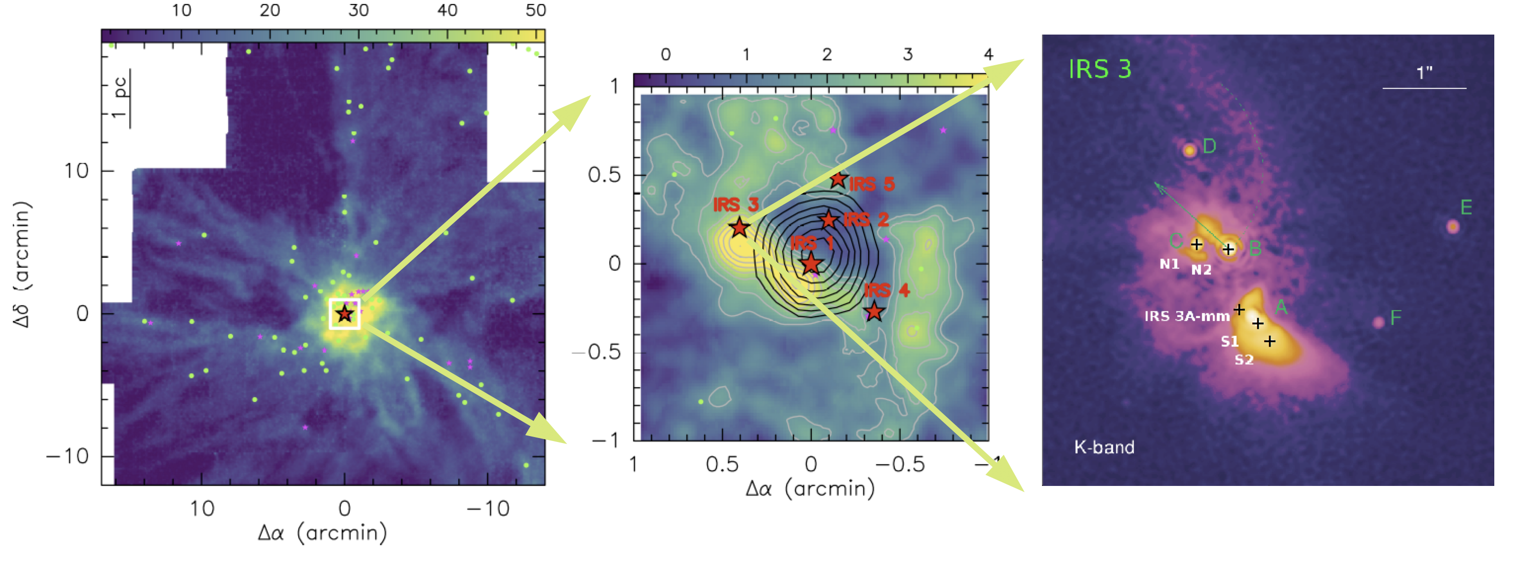
Figure 1: Left: Hub-filament system in Mon R2 as seen with the ¹³CO (1–0) molecular emission (Treviño-Morales et al., 2019). The white box corresponds to the inner 0.7 pc $\times 0.7$ pc around the cluster and zoomed in the right panel. Centre: Central hub of Mon R2 as seen with the H¹³CO⁺ (3→2) molecular emission (in colours and gray contours) tracing the high-density molecular gas (Treviño-Morales et al., 2014). The black contours corresponds to the H$\alpha 41$ emission tracing the HII region (Treviño-Morales et al., 2019). The red star gives the positions of the IRS 1-5 infrared sources.The colored symbols are the sources identified by Rayner et al. (2017): pink stars are protostars, and the green circles are bound clumps. Right: Color representation of the K band speckle image reported by Preibisch et al. (2002). Green letters correspond to the NIR sources as reported by Preibisch et al. (2002). Black crosses with white labels correspond to the positions listed in Table 1 that we have defined for an easier comparison with observations.

All the mm studies carried out. thus far towards IRS 3 were performed with single-dish observations or interferometric observations which are unable to resolve the IRS 3 mini-cluster (see (Boonman et al., 2003; van der Tak et al., 2003; Dierickx et al., 2015). Recently, Dungee et al. (2018) observed the $\nu_{3}$ ro-vibrational band of SO₂ confirming the existence of hot molecular gas (T_k=234$\pm$15 K) towards IRS 3, and derived a high SO₂abundance ($\sim$ a few 10^-7). Based on high spatial resolution continuum and spectroscopic ALMA observations, in the following we investigate the kinematics (Sect. 3.3) and chemistry (Sect. 4) of this massive protostar that is a reference for massive star formation studies.

Table 1: Positions.

Position	RA	DEC
N1	06:07:47.880	$-$06:22:55.42
N2	06:07:47.855	$-$06:22:55.49
IRS 3 A - mm	06:07:47.847	$-$06:22:56.21
S1	06:07:47.833	$-$06:22:56.36
S2	06:07:47.822	$-$06:22:56.58

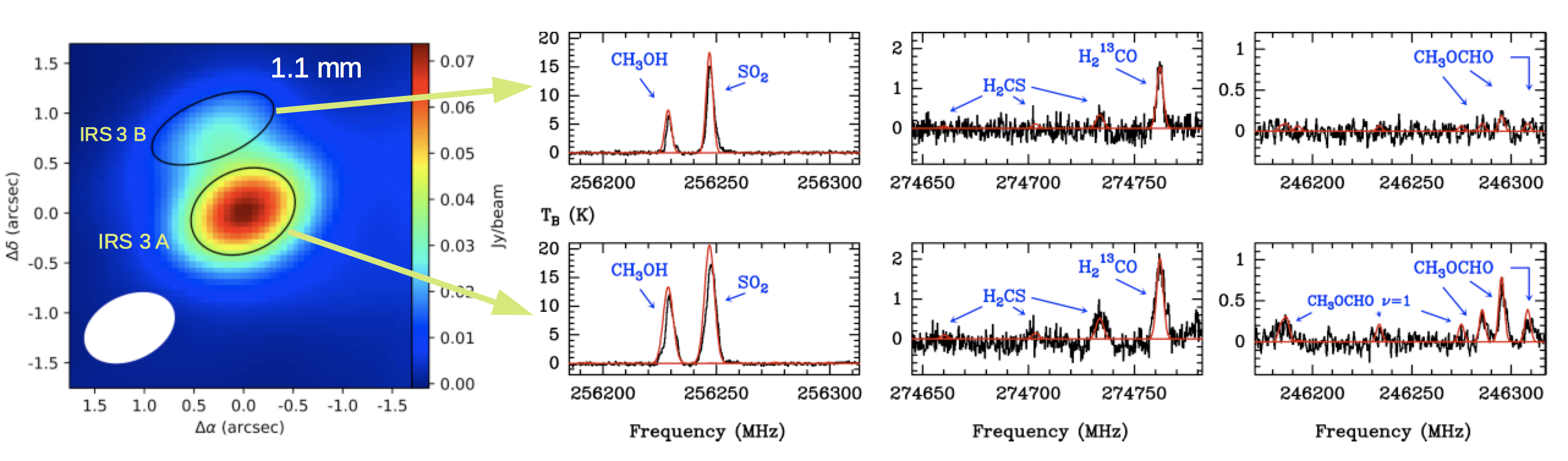
Figure 2: Left: Continuum image created by merging the bands centered at 262 GHz and 272 GHz (1.1 mm). The rms of the image is $\sigma$=3 mJy/beam. The black ellipses indicate the Half Power Beam Width of the Gaussians fitted to IRS 3 A (south) and IRS 3 B (north), respectively. Right) Example of the spectra observed towards IRS 3 A and IRS 3 B. .

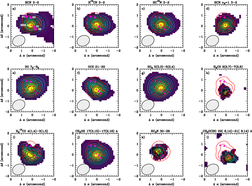
Figure 3: Line Integrated intensity maps calculated in the 0 to 20 km s^-1 velocity interval for all the lines except the HC₃N 30$\rightarrow$29 and CH₃OCHO 22(8,14)$\rightarrow$21(8,14) lines for which a narrower velocity range, from 5 to 15 km s^-1, was selected. All maps have been produced using an intensity threshold of 3$\sigma$. Contours (in black) correspond to 10% to 90% of the peak emission in steps of 10%. First contour and step are: a) 35.00 K km s^-1; b) 11.204 K km s^-1; c) 4.149 K km s^-1; d) 3.048 K km s^-1; e) 33.031 K km s^-1; f) 2.499 K km s^-1; g) 11.272 K km s^-1; h) 0.224 K km s^-1; i) 0.824 K km s^-1; j) 6.938 K km s^-1; k) 0.251 K km s^-1; l) 0.174 K km s^-1. The beam is shown in the left-bottom. corner. We have superposed in red contours the continuum emission at 1.1 mm (levels are 15, 30, 60, 90 mJy/beam). Stars indicate the positions N2, N1, S1, and S2 in Table 1. The cross indicates the position of the millimeter source IRS 3 A.

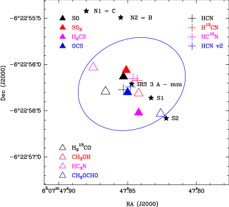
Figure 4: Scheme showing the positions of the emission centroids of the transitions shown in Fig. 3. Blue ellipse indicates a beam of 1.20$"$$\times$0.96$"$ P.A. $-$65^∘. Positions are labeled as in Fig. 1

2 Observations

The IRS 3 massive protostar was observed with ALMA (Atacama Large Millimeter/submillimeter Array) during Cycle 3. The observations were performed on April 2015 within the project 2015.1.00453.S. The project was observed with the 12m array, with the C40-4 configuration using 36 antennas. We used the Band 6 receiver in two different tunings corresponding to two different science goals: setup 1 centered at 259.0 GHz and 272.0 GHz in the lower and upper side band, respectively, and setup 2 centered at 249.0 and 262.0 GHz. A total of 18 spectral windows were observed, each with a spectral resolution $<$0.3 km s^-1 which allows to fully resolve the profiles of the detected lines (see Table 5). Total time on-source is 44.88 min for setup 1 and 53.3 min for setup 2. The phase calibrator was J0607-0834 and the quasar J0522-3627 was observed for bandpass and flux calibration. The data were calibrated using the ALMA pipeline in the version 4.7 of The Common Astronomy Software Applications (CASA; McMullin et al., 2007). Spectroscopic images of all spectral windows were produced in CASA using natural weighting. In the case of the higher signal-to-noise ratio (SNR) continuum images, we used Briggs weighting (robust=0.5) to achieve higher spatial resolution. Table 5 gives the frequency ranges of each spectral window and the final beams. For analysis purposes we used the CLASS/GILDAS package (Pety, 2005). The intensities are given in units of temperature.

3 Results

3.1 Continuum images

We have constructed continuum images at 1.2mm and 1.1mm by averaging the channels free from line emission in each band, and then merging the visibilities of the 247 GHz + 257 GHz and 262 GHz + 272 GHz bands, respectively. Total fluxes are S(1.1mm)= 168$\pm$25 mJy and S(1.2mm)= 135$\pm$6 mJy, which implies a spectral index, $\alpha$=3.7$\pm$3.3, consistent with the emission being dominated by dust thermal emission. Fig. 2 shows the higher spatial resolution continuum image at 1.1mm which barely resolves two millimeter clumps, hereafter IRS 3 A and IRS 3 B. The position of the millimeter source IRS 3 A is shifted by $\sim$0.38$"$ NE from the NIR position A as observed in K band by Preibisch et al. (2002) (see Fig. 1). The millimeter source IRS 3 B includes the NIR sources B and C which are indistinguishable with the angular resolution of our observations. We do not detect any millimeter compact emission towards sources D and E. Based on our millimeter observations, we estimate the total gas and dust mass in Mon R2 IRS 3 using a gray-body model,

$$M=\frac{F_{1.1mm}D^{2}}{B_{1.1mm}(T_{\rm dust})k_{1.1mm}}$$ (1)

where M is the gas+dust mass, $D$ is the distance, and we adopt a grain emissivity, $k_{1.1mm}$ = 0.0078 cm² g^-1, which is the value calculated by Ossenkopf & Henning (1994) for bare grains and dense gas, where gas-to-dust ratio of 100 is assumed. Adopting T_dust = 200 K (see Sect. 4), we derive a total mass of $\sim$0.14 M_⊙. The angular resolution of the 1.1mm image is not enough to cleanly discern between IRS 3 B and IRS 3 A. We have fitted two 2D Gaussians to the 1.1mm image to estimate the contribution of each source to the total flux (see Table 6). We obtain that $\sim$80% of the total flux comes from IRS 3 A, while only $\sim$20 % comes from the northern mm source. However our fit cannot account for the total flux, proving the existence of a more complex structure and an extended component. We adopt the flux and the half power full size of the brightest Gaussian to estimate the averaged H₂ column density towards IRS 3 A, N(H₂)$\sim$2.6$\times$10²³ cm^-2. An independent estimation of N(H₂) can be done from spectroscopic observations. Dungee et al. (2018) estimated N(¹³CO)=(1.1$\pm$0.2)$\times$10¹⁷ cm^-2 based on the absorption NIR lines towards IRS 3 A. Absorption lines are only probing the gas between the continuum source and the observer (in front of the continuum source). However, dust continuum emission is tracing the gas along the whole line of sight, i.e. in front the continuum source and beyond it. Assuming a standard ¹³CO abundance of $\sim$2$\times$10^-6 and that the amount of gas beyond the protostar is the same as that measured by the absorption lines, we derive N(H₂)$\sim$1.1$\times$10²³ cm^-2 along the line of sight which is in reasonable agreement with our estimate based on the 1.1mm continuum.

Table 2: List of the lines identified in IRS 3

Transition	Rest freq.	Eu	Log10 (Aij)
	(MHz)	(K)	(s-1)
C2H N=3$\rightarrow$2 J=7/2$\rightarrow$5/2	262004.26	25	-4.28
Cyanopolynes
HCN 3$\rightarrow$2	265886.43	25	-3.07
HCN $\nu_{2}$=1 3$\rightarrow$2	265852.76	1050	-2.64
H13CN 3$\rightarrow$2	259011.80	25	-3.11
HC15N 3$\rightarrow$2	258157.00	25	-3.12
HNC 3$\rightarrow$2	271981.14	26	-3.03
HC3N 30$\rightarrow$29	272884.75	203	-2.79
Sulphuretted species
SO 76$\rightarrow$65	261843.68	47	-3.63
SO 66$\rightarrow$55	258255.83	56	-3.67
SO2 5(3,3)$\rightarrow$5(2,4)	256246.95	36	-3.97
SO2 10(5,5)$\rightarrow$11(4,8)	248830.82	112	-4.66
SO2 31( 9,23)$\rightarrow$32( 8,24)	247169.77	654	-4.50
34SO2 3(3,1)$\rightarrow$3(2,2)	247127.39	27	-4.22
OCS 21$\rightarrow$20	255374.46	135	-4.31
OC34S 23$\rightarrow$22	272849.96	157	-4.23
H2CS 8(2,7)$\rightarrow$7(2,6)	274703.35	112	-3.54
H2CS 8(3,6)$\rightarrow$7(3,5)	274732.97	178	-3.58
H2CS 8(3,5)$\rightarrow$7(3,4)	274734.40	178	-3.58
CO-H species
H213CO 4(1,4)$\rightarrow$3(1,3)	274762.11	45	-3.26
HDCO 4(2,2)$\rightarrow$3(2,1)	259034.91	63	-3.44
CH3OH 16(- 2,15)$\rightarrow$15(- 3,13) E	247161.95	338	-4.59
CH3OH 4( 2, 2)$\rightarrow$5( 1, 5) A	247228.58	61	-4.67
CH3OH 16(3,13)$\rightarrow$16(2,14) A	248885.48	365	-4.08
CH3OH 17( 3,15)$\rightarrow$17( 2,16) A	256228.71	404	-4.05
CH3OH 25(- 1,24)$\rightarrow$25(- 0,25) E	271933.60	775	-4.26
COMS
CH3OCHO $\nu$ = 1 20( 8,13)$\rightarrow$19( 8,12) E	246184.18	353	-3.72
CH3OCHO $\nu$ = 1 21( 2,19)$\rightarrow$20( 2,18) A	246187.02	327	-3.66
CH3OCHO $\nu$ = 1 20( 7,13)$\rightarrow$19( 7,12) A	246233.57	344	-3.70
CH3OCHO $\nu$ = 1 20( 7,13)$\rightarrow$19( 7,12) E	246274.89	343	-3.70
CH3OCHO 20(11, 9)$\rightarrow$19(11, 8) E	246285.40	204	-3.80
CH3OCHO 20(11,10)$\rightarrow$19(11, 9) A	246295.13	204	-3.80
CH3OCHO 20(11,9)$\rightarrow$19(11, 8) A	246295.13	204	-3.80
CH3OCHO 20(11,10)$\rightarrow$19(11, 9) E	246308.27	204	-3.80
CH3OCHO $\nu$ = 1 20( 7,14)$\rightarrow$19( 7,13) E	247147.12	343	-3.69
CH3OCHO 21(14, 8)$\rightarrow$20(14, 7) E	258142.09	266	-3.84
CH3OCHO 21(13, 8)$\rightarrow$20(13, 7) E	258274.95	248	-3.79
CH3OCHO 21(13, 8)$\rightarrow$20(13, 7) A	258277.43	248	-3.79
CH3OCHO 21(13, 9)$\rightarrow$20(13, 8) A	258277.43	248	-3.79
CH3OCHO 21(13, 9)$\rightarrow$20(13, 8) E	258296.30	248	-3.79
CH3OCHO $\nu$ = 1 21(7,14)$\rightarrow$20(7,13) A	259003.87	356	-3.63
CH3OCHO $\nu$ = 1 21(7,14)$\rightarrow$20(7,13) E	259025.83	356	-3.63
CH3OCHO 22( 8,15)$\rightarrow$21( 8,14) A	273135.04	192	-3.57
CH3OCHO 22( 8,14)$\rightarrow$21( 8,13) E	273142.74	192	-3.58
CH3OCHO 22( 8,15)$\rightarrow$21( 8,14) E	273151.24	192	-3.58
CH3OCHO 22( 8,14)$\rightarrow$21( 8,13) A	273180.43	192	-3.57
CH3OCHO $\nu$ = 1 22(6,17)$\rightarrow$21(6,16) E	273653.25	361	-3.55
CH3OCH3 16( 1,15)-15( 2,14) EE	273107.18	127	-4.06
CH3OCH3 15( 5,10)-15( 4,11) EE	261248.11	144	-4.07
CH3OCH3 15( 5,10)-15( 4,11) AA	261250.49	144	-4.06
CH3OCH3 15( 5,11)-15( 4,12) EE	261956.62	144	-4.06

3.2 Spectroscopic observations

To study the chemical content of IRS 3, we have extracted the interferometric spectra towards IRS 3 A and IRS 3 B. Eye inspection reveals that the spectra towards IRS 3 A are more crowded than those towards IRS 3 B (see Fig. 2), thus confirming that the hot core is associated with the mm source IRS 3 A. The lines have been identified using the $"$The Cologne Database for Molecular Spectroscopy$"$ (CDMS) (Müller et al., 2005; Endres et al., 2016) and the "Jet Propulsion Laboratory Line catalogue" (JPL) (Pickett et al., 1998). We have adopted the 4$\sigma$ level in integrated intensity as the detection limit.

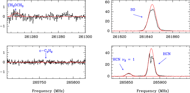
Figure 8: The same as Fig. 7.

The list of identified lines is shown in Table 2. We can divide the detected species in different families according with their chemical similarities: (i) the small hydrocarbon C₂H ; (ii) the nitrogenated carbon chains HCN, HNC, H¹³CN, HC¹⁵N, and HC₃N; (iii) the S-bearing species SO, SO₂, ³⁴SO₂, OCS, H₂CS, and OC³⁴S; and (iv) the organics CH₃OH, HDCO, and H₂¹³CO, and COMs such as methyl formate (CH₃OCOH) and dimethyl ether (CH₃OCH₃). The detections of these species are robust. We have checked the identification of the S-bearing species by searching for the ³⁴S isotopologues to test that the (non-)detections of all the ³⁴S isotopologues are compatible with a standard ratio of ³²S/³⁴S=22.5 (Wilson & Rood, 1994; Chin et al., 1996). The most doubtful identification is dimethyl ether. We have identified 4 lines that can be assigned to CH₃OCH₃ but three of them overlapped. In order to confirm (reject) this detection, we produced a synthetic spectrum assuming Local Thermodynamic Equilibrium and T_ex=170 K and checked that the obtained spectrum is compatible with the observed spectra (see Sect. 4 and Figs. 7 to Fig. 8). The COMs CH₃OCHO and CH₃OCH₃ are only detected towards IRS 3 A proving that the hot core is associated to this protostar.

Different line profiles can be observed in the spectra shown in Figs. 7 to  8, revealing that the observed lines come from different regions along the line of sight. The C₂H 3$\rightarrow$2 and HNC 3$\rightarrow$2 lines present intense absorptions towards the continuum compact source. A small feature in absorption is also detected at the frequency of the c-C₃H₂ 4_4,1$\rightarrow$3_3,0 line (see Fig. 8). Previous works in the (sub-)millimeter range showed that HNC, C₂H and c-C₃H₂ are abundant species in the surrounding molecular cloud with bright emission of the HNC 3$\rightarrow$2 and C₂H 3$\rightarrow$2 lines (Pilleri et al., 2013; Treviño-Morales et al., 2014, 2019). These absorptions are more likely produced by the cold gas in the envelope which absorbs the continuum and line emission from the hot core, and are not of interest for the goals of this paper. It should be noticed that our observations are filtering the extended emission, thus producing negative contours in the emission of these molecules also far from the compact hot core. Signatures of missed flux are also found in the HCN 3$\rightarrow$2, H¹³CN 3$\rightarrow$2, and to a lesser extent in the SO 6₆$\rightarrow$5₅ and 7₆$\rightarrow$6₅ images. Contrary to C₂H and HNC, these molecules present intense compact emission towards IRS 3 A and we keep them in our study. We recall that we are interested in the emission coming from the hot core that is not affected by the spatial filtering. Linewidths of $\sim$4 km s^-1 to $\sim$10 km s^-1 are measured in the detected lines. These linewidths are not correlated with the line excitation conditions. In fact, the more abundant species such as HCN, SO, and CH₃OH present wider profiles suggesting that they are the consequence of higher opacities and hence, higher sensitivity to the lower gas column densities measured at high velocities. A different case would be the vibrational excited line of HCN that is indeed probing the hottest regions of this disk and outflow system. In addition to larger linewidths, the HCN 3$\rightarrow$2, SO 6₆$\rightarrow$5₅ and 7₆$\rightarrow$6₅ lines show high velocity wings which extend from $-$15 km s^-1 to $\sim$22 km s^-1, suggesting that these lines could be partly tracing the outflow detected in IRS 3 by Dierickx et al. (2015). It is remarkable the non-detection of HC¹⁸O⁺ and N¹⁵NH⁺ J=3$\rightarrow$2 lines. These molecular ions are not expected to be abundant in hot cores (see e.g. Crockett et al., 2014). The high gas temperatures measured in this region (van der Tak et al., 2003; Dierickx et al., 2015; Dungee et al., 2018), and the detection of methyl formate confirm the existence of a hot core associated with Mon R 2 IRS 3, already suggested by Dierickx et al. (2015) that now we can identify with IRS 3 A.

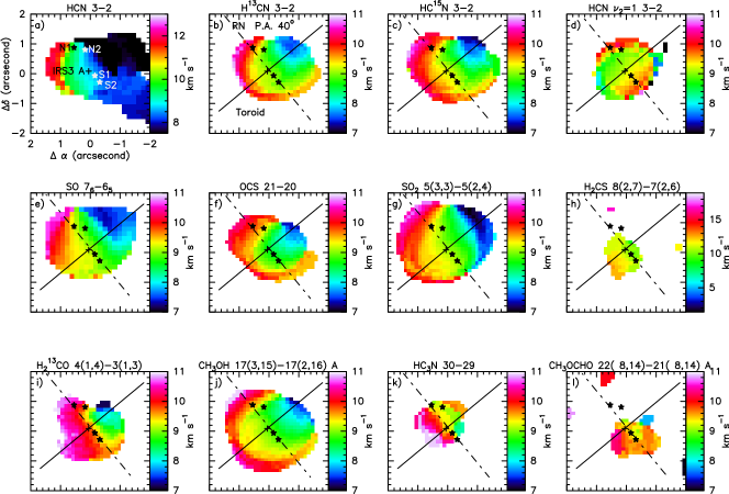
Figure 5: First-moment maps of the most intense lines detected in ALMA data. Straight lines in panel b) indicate the directions of the Position-Velocity diagrams in the directions perpendicular to the NIR nebula (toroid) and along it (RN, P.A. 40^∘). The beams are the same as in Fig. 3.

3.3 Moment maps

The integrated intensity maps (zeroth-moment maps) of the most intense lines are shown in Fig. 3. We exclude C₂H 3$\rightarrow$2 and HNC 3$\rightarrow$2 in these maps because, as commented before, their absorptions are coming from the surrounding envelope. Since this paper is focused on the kinematics and chemistry of the hot core, we are not going to further discuss these species. The emission of the rest of lines is centered on the vicinity of IRS 3 A, and is, in general, more extended than the dust emission. There are some differences between the spatial distributions of the different species. It is remarkable that the emission of H₂CS and CH₃OCHO are more intense in the southern part of the NIR nebula, with the emission of the CH₃OCHO line being maximum towards S2. In contrast, the emission of HC₃N is more intense in the northern nebula. Fig. 4 shows a scheme with the locations of the emission peaks of the different molecules. Most of the observed species peak in a region R$<$0.3" from IRS 3 A. Interestingly the emission of HCN and their isotopologues show the best agreement with the position of the continuum peak (labeled "IRS 3 A-mm" in Fig. 4). The peak of the CH₃OCHO is located $\sim$0.5$"$ SW to IRS 3 A-mm, that is about a half of the HPBW of our observations. The peak of the HC₃N emission is displaced by $\sim$0.5$"$ NE from IRS 3 A-mm. These displacements prove the chemical complexity of the IRS 3 hot core with at least two components, the brightest one associated to the torus that is forming the reflection nebula, and the second one originated in the NIR reflection nebula.

Relevant information on the structure and kinematics of the molecular gas can also be obtained from the first-moment maps shown in Fig. 5. First-moment maps show the intensity-weighted average velocity at every position, hence providing information on the emitting gas kinematics. Most of the first-moment maps present a clear SE-NW velocity gradient in the v_lsr=7$-$11 km s^-1 velocity range. The protostar IRS 3 A cannot be surrounded by a thick spherical envelope because it is associated to a bipolar NIR nebula. The detected velocity gradient is consistent with the emission coming from a toroidal envelope and/or a disk that is rotating in the direction perpendicular to the axis defined by the NIR nebula (the direction of the reflection nebula associated to IRS 3 A is P.A.$\sim$ 40^∘ and we will refer to it as "RN", hereafter). The v_lsr=7$-$11 km s^-1 velocity gradient is not detected in the HCN $\nu_{2}$=1 J=3$\rightarrow$2 and CH₃OCHO first-moment maps. We recall that the CH₃OCHO emission peaks towards the southern reflection nebula, suggesting a different origin. Moreover, the emission is red-shifted relative to the systemic velocity, v_sys $\sim$ 9 km s^-1, consistent with the interpretation that this line is associated to the walls of the cavity excavated by the CO outflow reported by Dierickx et al. (2015)). In the case of HCN $\nu_{2}$=1, although it is very marginal with the angular resolution of the observations, there seems to be a velocity gradient along the reflection nebula.

To further explore the kinematics of the molecular gas and distinguish between a toroidal envelope from the circumstellar disk, we have performed Position-Velocity (PV) diagrams in the direction perpendicular to the reflection nebula ("toroid" in Figs. 5b). In Fig. 6, we compare these PV-diagrams with the velocity patterns expected in the case of Keplerian rotation (red line) and solid-body rotation (black line). Only HCN and H${}_{2}^{13}$CO present a "butterfly" shape that could be interpreted as Keplerian rotation. For comparison we have plotted the Keplerian curve expected for M=40 M_⊙ and $i$ = 45^∘. Preibisch et al. (2002) provided an estimation of the masses of the NIR protostars. Assuming that the NIR sources A, B and C are driving the toroid rotation, the stellar mass would be 25-37 M_⊙. Yet, we can be missing an embedded protostar(s) that remains invisible at NIR wavelengths. We adopted 40 M_⊙ as a first approximation to the total stellar mass. The Keplerian velocity depends on the $M_{stars}\cdot sin(i)$ where $i$ is the unknown inclination angle of the toroid. Therefore, there is a degeneration between the total stellar mass and the inclination angle. We find a reasonable agreement with HCN and H${}_{2}^{13}$CO observations assuming $M_{stars}=40M_{\odot}$ and $i=45^{\circ}$. It should be noticed that a small change in the stellar mass could be compensated by a slight change the inclination angle. The match between the Keplerian curves thus obtained and the PV diagrams of HCN and H${}_{2}^{13}$CO is reasonable in the NW region but poor in the SE. As commented above, we cannot discard some contribution of an unresolved component of the molecular outflow detected by Dierickx et al. (2015) to the high velocity gas. The PV-diagram of the rarer isotopologue HC¹⁵N is more consistent with solid-body rotation. Solid-body rotation is expected if the emission is coming from a rotating ring. In the cases of unresolved disks, where the sensitivity is not enough to detect the highest rotation velocities expected close to the star, a Keplerian disk and solid-body rotation would be difficult to differentiate. Thus, the non detection of HC¹⁵N at high velocities might be a sensitivity problem since HCN/HC¹⁵N$\sim$ 300 (Hily-Blant et al., 2013). Solid-body rotation is also compatible with the PV diagrams of SO, SO₂, OCS, CH₃OH, and HC₃N. One would expect chemical gradients within the ring with the N(SO₂)/N(SO) and N(CH₃OH)/N(H₂CO) ratios increasing inwards (Gieser et al., 2019) but the limited angular resolution and sensitivity of our observations do not allow to discern it.

The emission of the HCN $\nu_{2}$=1 J=3$\rightarrow$2 line is centered on IRS 3 A with linewidths of $\sim$10 km s^-1. The HCN $\nu_{2}$=1 emission is unresolved in the direction of the toroid, but presents some extension to the north along the outflow direction (see Fig. 5). In order to explore the details of the kinematics of the hot gas traced by the vibrationally excited HCN line, we performed a PV diagram along the outflow direction ("RN" in Figs. 5b). The PV diagram shows an essentially unresolved emission without any clear evidence of a velocity gradient along this axis. On the other hand, the high excitation conditions of the HCN $\nu_{2}$=1 line and the large linewidths observed would also be consistent with the emission coming from the inner disk region. Given that the emission of the HCN $\nu_{2}$=1 is not resolved, we could not disentangle between these two physical processes.

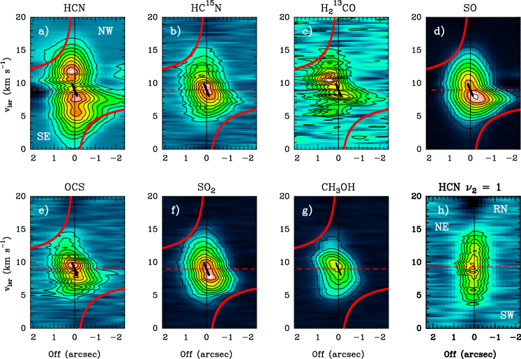
Figure 6: a), b), c), d), e), f), and g): Position-Velocity (PV) diagrams along the axis perpendicular to the nebula (toroid in Fig. 5). The red solid lines indicate the Keplerian velocity for a mass of 40 M_⊙ and an inclination i=45^∘ while the solid black line show the velocity pattern for a solid-body model. h) PV diagram along the direction of the NIR nebula (RN in Fig. 5) of the HCN $\nu_{2}$=1 3$\rightarrow$2 line. First contour and step (both share the same value) in each panel are: a) 3.72 K; b) 0.74 K; c) 0.25 K; d) 5.00 K; e) 0.56 K; f) 1.76 K; g) 1.77 K; h) 1.00 K.

4 Chemical content

The estimation of accurate molecular column densities requires the knowledge of the excitation conditions. The excitation temperature can be easily derived using the rotation diagram technique as long as several transitions are observed. We have identified several lines of SO, SO₂, CH₃OH, and CH₃OCHO in our interferometric spectra (see Table 2). The CH₃OCHO lines are weak and there is large overlapping between different transitions, hindering the estimation of the rotation temperature. The two SO lines have similar $E_{u}$ precluding an accurate estimate of T_rot. Therefore, we have used the SO₂ and CH₃OH lines to estimate the gas temperature. We obtained T_rot = 175${}_{-16}^{+15}$ K and N(SO₂)=3.4${}_{-0.5}^{+0.6}$ $\times$ 10¹⁶ cm^-2 using the three SO₂ lines observed towards IRS 3 A (see Table 3). A slightly lower value of the rotation temperature, T_rot = 129${}_{-9}^{+10}$ K, and N(CH₃OH)=1.1${}_{-0.2}^{+0.3}$ $\times$ 10¹⁷ cm^-2, are found using the methanol lines. These temperatures are consistent with those previously obtained by other authors. Boonman et al. (2003) derived T_ex=250${}_{-100}^{+200}$K based on the $\nu_{2}$ band of H₂O. Excitation temperatures of 110$\pm$20 K and 125$\pm$35 K for CH₃OH and SO₂, respectively, were estimated by van der Tak et al. (2003) on the basis of single-dish observations. Dierickx et al. (2015) estimated T_ex= 126$\pm$ 22 K toward IRS 3 from the CH₃CN line emission. Dungee et al. (2018) obtained T_ex=234$\pm$15 K from $\nu_{3}$ ro-vibrational band of SO₂. We can conclude that the observed excitation temperatures ranges from $\sim$110 K using millimeter single-dish observations to T_ex=250 K when using the infrared ro-vibrational bands, suggesting a temperature gradient along the line of sight.

The SO₂ column density derived from our data is in good agreement with that obtained by Dungee et al. (2018). However, we do not obtain a good fit to the three millimeter lines observed, which is the consequence of the steep gas temperature gradient along the line of sight (see Figs. 7). We cannot obtain a good fit to all the methanol lines using a single rotation temperature, either. Given the small number of transitions observed, we do not consider that we could obtain realistic results using a more complex fitting with several rotation temperatures. The molecular column densities of the rest of species have been derived by fitting the lines observed towards IRS 3 A assuming Local Thermodynamic Equilibrium (LTE), which is a reasonable assumption for the high densities (n(H₂)$>$10⁷ cm^-3) expected in a hot core. Taking into account the high SNR ($>>$10) in most of the lines, the main uncertainties in the derived column densities would come from the adopted rotation temperatures. We estimate these uncertainties by calculating the column densities with two temperatures, 129 K -170 K, that are representative of the temperatures derived using different molecular tracers (see Table 3). The uncertainties thus obtained are of $\sim$20%-25% for most species, except for the vibrationally excited HCN for which the differnce is of more than one order of magnitude due its high excitation conditions. In Figs. 7 and  8, we show the results for T_k=170 K. The quality of the fit is essentially the same when using T_k=129 K and the column densities derived with this assumption. We have also derived an upper limit to the column densities of HC¹⁸O⁺ and N¹⁵N⁺ column densities based on the non-detection of the HC¹⁸O⁺ J=3$\rightarrow$2 lines. Our limit indicates that N(HCN)/N(HCO⁺)$\sim$8. This value has been calculated from thee H¹³CN and HC¹⁸O⁺ column densities assuming ¹²C/¹³C=60 (Savage et al., 2002) and ¹⁶O/¹⁸O=550 (Wilson & Rood, 1994). This high N(HCN)/N(HCO⁺) ratio is found in the innermost regions of the Class I disks and is interpreted as the result of the high densities and temperatures prevailing in these regions (Agúndez et al., 2008; Fuente et al., 2012; Crockett et al., 2014; Fuente et al., 2020).

Molecular abundances have been estimated adopting the value derived from our millimeter observations, N(H₂)=2.6$\times$10²³ cm^-2 (see Table 3). Abundances of $\sim$ a few 10^-7 are measured for HCN, CH₃OH, and SO₂. Our estimated SO₂ abundance is 5 times lower than that derived by Dungee et al. (2018) mainly due to the higher adopted value of N(H₂). We recall that the CH₃OH lines are very likely optically thick and the derived abundance a lower limit to the real value. Following our calculations, SO₂ accounts for a significant fraction, $\sim$1%, of the sulphur budget assuming the solar abundance, S/H=1.5$\times$10^-5 (Asplund et al., 2005). The abundance of SO₂ is a factor $>$5 higher than those of SO, OCS, and H₂CS. It would be noticed that our calculations of the column densities of SO₂ and OCS are not heavily affected by opacity effects. We have fitted the lines of the isotopologues ³⁴SO₂, OC³⁴S and derived N(XS)/N(X³⁴S) ratios $\sim$22.5 (see Table 3, and Fig. 7 and  8), proving that the lines of the main isotopologues are optically thin. Unfortunately, we do not have intense ³⁴SO lines in our interferometric spectra to estimate the opacity of the SO lines. We do not have interferometric observations of the abundant species, H₂S and CS, that would be useful to complete the inventory of S-bearing molecules. The sulphur chemistry in Mon R2 IRS 3 was previously investigated by van der Tak et al. (2003) using single-dish observations of a wider set of S-bearing molecules including H₂S. They found that SO₂ was the most abundance S-bearing molecule, suggesting that SO₂ is the most abundant "observable" S-bearing molecule in this protostar and the main sulphur reservoir in gas phasee.

5 Discussion

High spatial resolution observations show that hot cores are complex objects in which molecular species present differentiated spatial distributions (Zernickel et al., 2012; Qin et al., 2015; Rivilla et al., 2017; Bonfand et al., 2017; Palau et al., 2017; Allen et al., 2017; Tercero et al., 2018; Mininni et al., 2020; Gieser et al., 2021). One well-known example is the hot corino IRAS 16293-2422 which is formed by two protostars separated by 5$"$ ($\sim$14 au), and usually referred to as A and B, IRAS 16293–2422 A being the most intense in the emission of S-bearing species (Chandler et al., 2005; Caux et al., 2011). Recent observations at an angular resolution of 0.1$"$ ($\sim$700 au) revealed that IRAS 16293–2422 A is itself a multiple source with complex kinematics and chemistry (Oya & Yamamoto, 2020). Interferometric studies using large millimeter telescopes like ALMA are therefore required to have a more precise view of the molecular chemistry in these objects. We present high spatial resolution ALMA observations of the hot core Mon R 2 IRS 3. Our interferometric images show that the Mon R 2 IRS 3 is formed by two mm cores, IRS 3 A and IRS 3 B. The molecular emission is mainly associated with IRS 3 A, which seems to be the one that harbors the hot core. The protostar IRS 3 A itself present a complex structure in which we identify at least two components: i) most species such as HCN (and its isotopologues), SO, SO₂, OCS, H${}_{2}^{13}$CO and CH₃OH comes from the rotating ring that is forming the nebula; ii) the emission of the H₂CS and CH₃OCHO lines come from the southern NIR nebula; iii) the emission of HC₃N is shifted to the north. In addition, the detailed analysis of the PV diagrams suggests that there could be chemical differentiation within the ring, with N(SO)/N(SO₂) and N(CH₃OH)/N(H₂CO) increasing inwards. However, we should put a word of caution in this result since the SO and CH₃OH lines might be optically thick.

Chemical models predict that the abundances of sulphur-bearing species are expected to be enhanced in hot cores (e.g., Charnley, 1997; Hatchell et al., 1998; Viti et al., 2004; Herpin et al., 2009; Wakelam et al., 2011; Vidal & Wakelam, 2018). During the collapse, the bulk of the sulphur reservoir is locked onto grain mantles (see e.g. Vidal et al., 2017; Navarro-Almaida et al., 2020). These species are released to the gas phase again when dust temperatures increase to $>$100 K and the ice mantles are evaporated in the hot core/corino stage. Then, an active S-chemistry is initiated where SO₂ is a direct product of SO, through the radiative association of O and SO and the neutral-neutral reaction of SO with OH, making the SO/SO₂ ratio decrease as the hot core/corino evolves. Dungee et al. (2018) observed the $\nu_{3}$ ro-vibrational band of SO₂ confirming the existence of hot molecular gas (T_k=234$\pm$15 K) towards IRS 3, with a high SO₂ abundance ($\sim$ a few 10^-7). The detection of SO, OCS, H₂CS and SO₂ in our interferometric images, provides a more complete view of the sulphur chemistry in this hot core. The N(SO)/N(SO₂) ratio is $\sim$0.29 in IRS 3 A similar to that observed in the Orion hot core and AFGL 2591 VLA 3 (see Table 4). Similar values of N(SO)/N(SO₂) are also found in a significant fraction of the massive protostellar objects imaged within the The NOrthern Extended Millimeter Array (NOEMA) large program “Fragmentation and disk formation during high-mass star formation" (CORE) (Gieser et al., 2021). Based only in this ratio, one could think that the IRS 3 A presents the characteristic chemistry of an evolved hot core such as Orion KL. However we find a great difference when comparing the abundances of COMs in IRS 3 A and Orion, the COMs being more abundant in Orion. For instance, N(SO₂)/N(CH₃OCHO)$\sim$0.38 in Orion and N(SO₂)/N(CH₃OCHO)$\sim$11 in IRS 3 A (see Table 4 ). One possibility is that the CH₃OCHO lines are optically thick and we are underestimating their column densities. Another possibility is that the N(SO)/N(SO₂) ratio is overestimated because the SO lines are optically thick, and the hot core is in an earlier evolutionary stage. A more complete study of chemistry of IRS 3 A , including isotopologues, is required for an accurate comparison.

We should also consider the possibility that the high abundance of SO₂ in IRS 3 A is produced by the shocks associated with outflow(s) of the region. Indeed shock chemistry successfully explain the gas-phase SO₂ abundance measured toward the Orion Plateau, which shows very broad lines indicative of shocks generated by Orion IRC 2 outflows (Blake et al., 1987; Esplugues et al., 2013; Esplugues et al., 2014; Crockett et al., 2014). Shocks can sputter dust grains (May et al., 2000; Holdship et al., 2016), leading to the release of more sulphur and subsequent SO₂ formation. Recent interferometric observations of S-bearing species towards the outflows associated with L 1157 (Feng et al., 2020) and NGC 1333 IRAS 4 (Taquet et al., 2020) showed important gradients in the SO/SO₂ ratio along the outflows that were interpreted in terms of time evolution, with SO₂ being more abundant at later stages (Taquet et al., 2020; Feng et al., 2020). Indeed, shocks could also produce enhanced abundances of COMs in intermediate-mass and massive protostars (see, e.g., Palau et al., 2011, 2017). We cannot therefore discard that the SO₂ emission towards IRS 3 A has some contribution from shocked gas close to the star. However, the SO₂ lines toward Mon R 2 IRS 3 A are substantially narrow $\Delta V\sim$ 4 km s^-1, compared with the high velocities observed in the bipolar outflow detected by Dierickx et al. (2015). Moreover, the PV diagrams of the S-bearing species are similar to those of HC¹⁵N without any signature of a different origin (see Fig. 6). Our results are therefore more consistent with the interpretation that sulphur has been released from the ices due to radiative heating (or perhaps mild shocks) rather than sputtered by strong shocks.

Although a large theoretical and observational effort has been undertaken in the last five years to understand sulphur chemistry, there is still a big debate about the main sulphur reservoirs in gas phase and volatiles, and eventually about the sulphur elemental abundance in molecular clouds (Fuente et al., 2016; Vidal et al., 2017; Fuente et al., 2019; Le Gal et al., 2019; Laas & Caselli, 2019; Navarro-Almaida et al., 2020; Shingledecker et al., 2020; Bulut et al., 2021)). According to chemical models, SO and SO₂ are the main gas-phase sulphur reservoirs in gas phase under the conditions of high temperature and density prevailing in hot cores (Esplugues et al., 2014; Vidal et al., 2017; Gieser et al., 2019). This is consistent with our findings since the abundance of SO₂ is a factor $>$5 higher than those of SO, OCS, and H₂CS. Summing the abundances of all S-bearing molecules detected towards IRS 3 A, we can account only for $\sim$ 1 % of the total sulphur budget. Even assuming that the abundances of H₂S and CS are similar to that of SO₂, only $\sim$ 3% of the sulphur is in gas molecules, i.e. , $>$ 95% should be locked in ices or refractories. However, one would not expect icy water at the high temperatures measured in this source. One possibility is that sulphur remains locked in allotropes (S₂, S₃, …, or the most stable S₈) as suggested by Jiménez-Escobar & Muñoz Caro (2011). Shingledecker et al. (2020) have shown that the inclusion of cosmic ray-driven radiation chemistry and fast non-diffusive bulk reactions in grain surface chemistry lead to a reduction in the abundance of solid. H₂S and HS, and a significant increase in the abundances of OCS, SO₂, and allotropes such as S₈ in the ice. Experiments and theoretical work is still needed to determine the solid reservoir of sulphur.

Table 3: Molecular column densities and abundances

Mol	Column densities (cm-2)		$\Delta V$(km s-1)	Abundance1
	Tk=129 K	Tk=170 K		relative to H2
HCN	8.7$\times$1014	1.1$\times$1015	10.0	4.2$\times$10-9
HCN $\nu_{2}$=1	3.5$\times$1017	6.0$\times$1016	10.0	2.3$\times$10-7
H13CN	2.4$\times$1014	3.0$\times$1014	7.0	1.1$\times$10-9
HC15N	9.0$\times$1013	1.1$\times$1014	6.0	4.2$\times$10-10
HC3N	1.7$\times$1013	1.5$\times$1013	4.0	5.8$\times$10-11
SO	8.0$\times$1015	1.0$\times$1016	7.0	3.8$\times$10-8
SO2∗	…	3.4$\times$1016	6.0	1.3$\times$10-7
34SO2	…	1.0$\times$1015	6.0	3.8$\times$10-9
OCS	3.0$\times$1015	2.5$\times$1015	6.0	9.6$\times$10-9
OC34S	8.8$\times$1013	8.7$\times$1013	6.0	3.3$\times$10-10
H2CS	9.0$\times$1013	8.0$\times$1013	4.0	3.1$\times$10-10
H213CO	4.5$\times$1014	6.0$\times$1014	6.0	2.3$\times$10-9
HDCO	1.2$\times$1014	1.5$\times$1014	4.0	5.7$\times$10-10
CH3OH∗	1.4$\times$1017	…	6.0	5.4$\times$10-7
CH3OCHO	2.5$\times$1015	3.0$\times$1015	4.0	1.1$\times$10-8
CH3OCH3	8.0$\times$1014	1.1$\times$1015	4.0	4.2$\times$10-9
HC18O+#	$<$ 1.6$\times$1012	$<$ 2.0$\times$1012	4.0	$<$8$\times$10-12
N15NH+#	$<$ 1.5$\times$1012	$<$ 1.8$\times$1012	4.0	$<$7$\times$10-12

Notes: ¹ Adopting N(H₂)=2.6$\times$10²³ cm^-2 derived in Sect. 3.1 and column densities derived with T_k=170 K, except for methanol; ^∗ We have derived these numbers using the rotational diagram technique (see text for details); ^# The rms has been derived in a channel of $\Delta v$=1 km s^-1. Then, the upper limit is calculated assuming a linewidth of 4 km s^-1 and imposing T_b$<$3$\times$rms.

Table 4: Comparison with other sources

Hot core	N(SO)/N(SO2)	N(OCS)/N(H2CS)	N(CH3OCHO)/N(CH3OH)	N(SO2)/N(CH3OCHO)	N(H2CS)/N(CH3OCHO)
IRS 3 A	$\sim$0.29	$\sim$31	$\sim$0.02	$\sim$11	$\sim$0.03
NGC 7129$-$IRS 2	$<$125	$\sim$7	$\sim$0.014	$\sim$0.16	$\sim$0.38
Orion	$\sim$1	$\sim$13	$\sim$0.26	$\sim$0.38	$\sim$0.01
AFGL 2591 VLA 3	$\sim$0.5	…	$\sim$0.05	$\sim$77	…

Note: We have adopted the molecular abundances for Orion and NGC 7129$-$IRS 2 reported by Fuente et al. (2014). The listed abundances towards NGC 7129$-$IRS 2 correspond to the average value in a region with a radius of D$\sim$0.008 pc centered on the continuum source. For the Orion hot core, the listed column densities are average values in a region of D$\sim$0.003 pc. For comparison, the spatial resolution of our observations is HPBW$\sim$(0.005$\times$0.003) pc. To derive N(SO) we have adopted N(SO)/N(S¹⁸O)=500 for Orion and NGC 7129$-$IRS 2 . Data for AFGL 2591 VLA 3 have been taken from Gieser et al. (2019). In this case, the synthesized beam is $\sim$0.007 pc and we have assumed that N(SO)/ N(SO₂)$\sim$N(³³SO)/N(³³SO₂).

6 Summary and conclusions

We present high angular resolution 1.1mm continuum and spectroscopic ALMA observations of the well-known massive protostellar cluster Mon R 2$-$IRS 3, that is composed of two components, IRS 3 A and IRS 3 B. The results can be summarized as follows:

1. Continuum observations show the presence of two components that are separated by $\sim$0.65$"$. These components are barely resolved by our 1.1mm observations (HPBW$\sim$ 1.2$"$ $\times$0.9$"$ ). We estimate that IRS 3 A is responsible of $\sim$80 % of the continuum flux.

2. Spectroscopic observations show that IRS 3 A has the crowded spectra typical of hot cores. In particular, we have detected intense lines of carbon chains such as HCN, H¹³CN, HC¹⁵N, HNC, and HC₃N, the organics CH₃OH, HDCO, and H₂¹³CO, the S-bearing species SO, SO₂, H₂CS, and OCS, and of the COMs, methyl formate (CH₃OCHO) and dimethyl ether (CH₃OCH₃).

3. Most species arise in a rotating ring centered on IRS 3 A. In contrast, the emission of COMs peak in the southern part of the NIR reflection nebula. The peak of the HC₃N emission is displaced by $\sim$0.5$"$ towards the North of the NIR nebula.

4. The position-velocity diagrams in the direction perpendicular to the NIR nebula reveal that the emission of most molecules comes from a rotating torus and/or a circumstellar. disk. The emission of the HCN $\nu_{2}$=1 3$\rightarrow$2 line remains unresolved and present a linewidth of $\sim$10 km s^-1. We interpret this emission as coming from the disk wind and/or the emergent outflow. The emission of methyl formate is located in the southern NIR nebula and is more likely associated to the interaction of the bipolar outflow with the molecular cloud.

5. Based on SO₂ we derive gas kinetic temperatures of T_k$\sim$ 170 K towards the IRS 3 A. The most abundant S-bearing species is SO₂ with an abundance of $\sim$ 1.3$\times$10^-7, and $\chi$(SO/SO₂) $\sim$ 0.29.

6. At the high temperatures prevailing in hot cores, all the icy mantles of grains are evaporated releasing their content to the gas phase. Following our calculations, SO₂ accounts for a significant fraction, $\sim$1%, of the sulphur budget. The abundance of SO₂ is a factor $>$5 higher than those of SO, OCS, and H₂CS. This implies that $>$95% of the sulphur should be locked in refractories or species such as S₂ and sulphur allotropes that cannot be observed.

Data availability

The data underlying this article will be shared on reasonable request to the corresponding author.

7 Acknowledgements

This paper makes use of the following ALMA data: ADS/JAO. 2016.1.00813.S. ALMA is a partnership of ESO (representing its member states), NSF (USA) and NINS (Japan), together with NRC (Canada), MOST and ASIAA (Taiwan), and KASI (Republic of Korea), in cooperation with the Republic of Chile. The Joint ALMA Observatory is operated by ESO, AUI/NRAO and NAOJ. We thank the Spanish MICINN for funding support from AYA2016-75066-C2-2-P and PID2019-106235GB-I00. SPTM and acknowledges to the European Union$\textquoteright$s Horizon 2020 research and innovation program for funding support given under grant agreement No 639459 (PROMISE) and Chalmers Gender Initiative for Excellence (Genie). A.S.M. acknowledges support from the Collaborative Research Centre (SFB) 956 (sub-project A6), funded by the Deutsche Forschungsmeneinschaft (DFG) - project 184018867

Appendix A Supporting material

Table 5: Observations

Continuum	Subbands (MHz)	Synthesized beam	PA(∘)	$\Delta v$ (km s-1)	rms (mJy/beam)
1.2mm	247 GHz+257 GHz	1.010$"$ $\times$0.676$"$	-64.61	4271.07	0.87
1.1mm	262 GHz+272 GHz	0.946$"$ $\times$0.634$"$	-64.96	3248.33	0.85
Spw	Freq. range (MHz)	Synthesized beam	PA(∘)	$\Delta v$ (km s-1)	rms (K)1
1	255363$-$255490	1.23$"$ $\times$0.97$"$	-65	0.25	0.145
2	256185$-$256313	1.23$"$ $\times$0.97$"$	-65	0.25	0.148
3	258127$-$258186	1.22$"$ $\times$0.97$"$	-65	0.25	0.156
4	258197$-$258313	1.22$"$ $\times$0.96$"$	-65	0.28	0.134
5	258983$-$259040	1.22$"$ $\times$0.97$"$	-66	0.25	0.179
6	271922$-$272040	1.18$"$ $\times$0.94$"$	-65	0.25	0.184
7	272835$-$272951	1.19$"$ $\times$0.94$"$	-65	0.27	0.169
8	273103$-$273219	1.17$"$ $\times$0.94$"$	-65	0.25	0.211
9	273550$-$273667	1.16$"$ $\times$0.94$"$	-65	0.25	0.183
10	274645$-$274782	1.16$"$ $\times$0.94$"$	-65	0.25	0.178
11	246171$-$246317	1.3$"$ $\times$1.0$"$	-65	0.30	0.103
12	247114$-$247260	1.3$"$ $\times$1.0$"$	-65	0.30	0.105
13	248820$-$248944	1.3$"$ $\times$1.0$"$	-65	0.25	0.102
14	261946$-$262050	1.22$"$ $\times$0.95$"$	-65	0.25	0.137
15	261242$-$261300	1.23$"$ $\times$0.95$"$	-65	0.25	0.180
16	261814$-$261873	1.23$"$ $\times$0.95$"$	-65	0.28	0.124
17	265702$-$265818	1.20$"$ $\times$0.96$"$	-65	0.28	0.127
18	265828$-$265945	1.20$"$ $\times$0.96$"$	-65	0.27	0.164

Note:¹ The rms of of the spectra towards. IRS 3 A which are shown in Fig. 7 and . 8.

Table 6: Gaussian fits to the continuum emission

RA(J2000)	Dec(J2000)	Major ($"$)	Minor($"$)	PA(∘)	S1.1mm (mJy/beam)
06:07:47.85	$-$06:22:56.27	1.09(0.01)	0.82(0.01)	65.6(0.6)	88.5(0.3)
06:07:47.87	$-$06:22:55.43	1.30(0.01)	0.60(0.01)	68.1(0.6)	25.9(0.3)

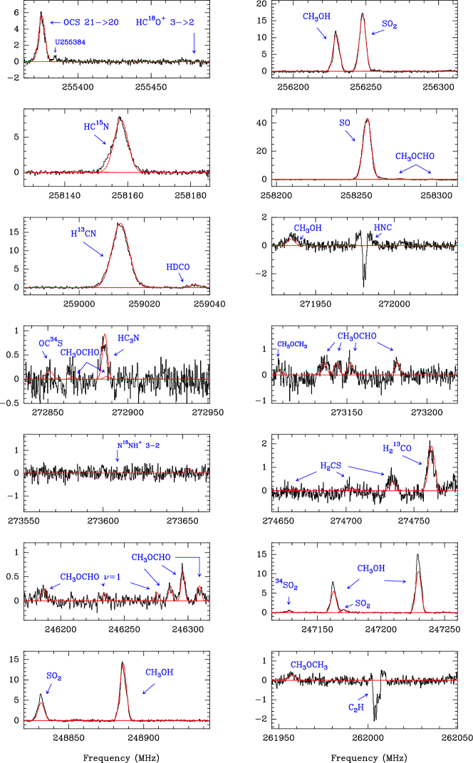
Figure 7: Interferometric spectra towards IRS 3 A. The LTE fitting described in Sect. 4 and Table3 is shown in red.

References

- Agúndez et al. (2008) Agúndez M., Cernicharo J., Goicoechea J. R., 2008, A&A, 483, 831
- Allen et al. (2017) Allen V., van der Tak F. F. S., Sánchez-Monge Á., Cesaroni R., Beltrán M. T., 2017, A&A, 603, A133
- Alvarez et al. (2004) Alvarez C., Feldt M., Henning T., Puga E., Brandner W., Stecklum B., 2004, ApJS, 155, 123
- Asplund et al. (2005) Asplund M., Grevesse N., Sauval A. J., 2005, in Barnes Thomas G. I., Bash F. N., eds, Astronomical Society of the Pacific Conference Series Vol. 336, Cosmic Abundances as Records of Stellar Evolution and Nucleosynthesis. p. 25
- Beckwith et al. (1976) Beckwith S., Evans II N. J., Becklin E. E., Neugebauer G., 1976, ApJ, 208, 390
- Beuther et al. (2002) Beuther H., Schilke P., Sridharan T. K., Menten K. M., Walmsley C. M., Wyrowski F., 2002, A&A, 383, 892
- Beuther et al. (2007) Beuther H., Churchwell E. B., McKee C. F., Tan J. C., 2007, in Reipurth B., Jewitt D., Keil K., eds, Protostars and Planets V. p. 165 (arXiv:astro-ph/0602012)
- Blake et al. (1987) Blake G. A., Sutton E. C., Masson C. R., Phillips T. G., 1987, ApJ, 315, 621
- Boley et al. (2013) Boley P. A., et al., 2013, A&A, 558, A24
- Bonfand et al. (2017) Bonfand M., Belloche A., Menten K. M., Garrod R. T., Müller H. S. P., 2017, A&A, 604, A60
- Boonman et al. (2003) Boonman A. M. S., Doty S. D., van Dishoeck E. F., Bergin E. A., Melnick G. J., Wright C. M., Stark R., 2003, A&A, 406, 937
- Bulut et al. (2021) Bulut N., et al., 2021, A&A, 646, A5
- Carpenter et al. (1997) Carpenter J. M., Meyer M. R., Dougados C., Strom S. E., Hillenbrand L. A., 1997, AJ, 114, 198
- Caux et al. (2011) Caux E., et al., 2011, A&A, 532, A23
- Chandler et al. (2005) Chandler C. J., Brogan C. L., Shirley Y. L., Loinard L., 2005, ApJ, 632, 371
- Charnley (1997) Charnley S. B., 1997, ApJ, 481, 396
- Chin et al. (1996) Chin Y. N., Henkel C., Whiteoak J. B., Langer N., Churchwell E. B., 1996, A&A, 305, 960
- Choi et al. (2000) Choi M., Evans Neal J. I., Tafalla M., Bachiller R., 2000, ApJ, 538, 738
- Crockett et al. (2014) Crockett N. R., et al., 2014, ApJ, 787, 112
- Didelon et al. (2015) Didelon P., et al., 2015, A&A, 584, A4
- Dierickx et al. (2015) Dierickx M., Jiménez-Serra I., Rivilla V. M., Zhang Q., 2015, ApJ, 803, 89
- Dungee et al. (2018) Dungee R., et al., 2018, ApJ, 868, L10
- Endres et al. (2016) Endres C. P., Schlemmer S., Schilke P., Stutzki J., Müller H. S. P., 2016, Journal of Molecular Spectroscopy, 327, 95
- Esplugues et al. (2013) Esplugues G. B., Tercero B., Cernicharo J., Goicoechea J. R., Palau A., Marcelino N., Bell T. A., 2013, A&A, 556, A143
- Esplugues et al. (2014) Esplugues G. B., Viti S., Goicoechea J. R., Cernicharo J., 2014, A&A, 567, A95
- Feng et al. (2020) Feng S., et al., 2020, ApJ, 896, 37
- Fuente et al. (2012) Fuente A., Cernicharo J., Agúndez M., 2012, ApJ, 754, L6
- Fuente et al. (2014) Fuente A., et al., 2014, A&A, 568, A65
- Fuente et al. (2016) Fuente A., et al., 2016, A&A, 593, A94
- Fuente et al. (2019) Fuente A., et al., 2019, A&A, 624, A105
- Fuente et al. (2020) Fuente A., Treviño-Morales S. P., Le Gal R., Rivière-Marichalar P., Pilleri P., Rodríguez-Baras M., Navarro-Almaida D., 2020, MNRAS, 496, 5330
- Garrod et al. (2008) Garrod R. T., Widicus Weaver S. L., Herbst E., 2008, ApJ, 682, 283
- Giannakopoulou et al. (1997) Giannakopoulou J., Mitchell G. F., Hasegawa T. I., Matthews H. E., Maillard J.-P., 1997, ApJ, 487, 346
- Gieser et al. (2019) Gieser C., et al., 2019, A&A, 631, A142
- Gieser et al. (2021) Gieser C., et al., 2021, arXiv e-prints, p. arXiv:2102.11676
- Ginard et al. (2012) Ginard D., et al., 2012, A&A, 543, A27
- Hackwell et al. (1982) Hackwell J. A., Grasdalen G. L., Gehrz R. D., 1982, ApJ, 252, 250
- Hatchell et al. (1998) Hatchell J., Thompson M. A., Millar T. J., MacDonald G. H., 1998, A&A, 338, 713
- Henning et al. (1992) Henning T., Chini R., Pfau W., 1992, A&A, 263, 285
- Herbst & van Dishoeck (2009) Herbst E., van Dishoeck E. F., 2009, ARA&A, 47, 427
- Herpin et al. (2009) Herpin F., Marseille M., Wakelam V., Bontemps S., Lis D. C., 2009, A&A, 504, 853
- Hily-Blant et al. (2013) Hily-Blant P., Pineau des Forêts G., Faure A., Le Gal R., Padovani M., 2013, A&A, 557, A65
- Holdship et al. (2016) Holdship J., et al., 2016, MNRAS, 463, 802
- Jiménez-Escobar & Muñoz Caro (2011) Jiménez-Escobar A., Muñoz Caro G. M., 2011, A&A, 536, A91
- Jiménez-Serra et al. (2013) Jiménez-Serra I., Báez-Rubio A., Rivilla V. M., Martín-Pintado J., Zhang Q., Dierickx M., Patel N., 2013, ApJ, 764, L4
- Koresko et al. (1993) Koresko C. D., Beckwith S., Ghez A. M., Matthews K., Herbst T. M., Smith D. A., 1993, AJ, 105, 1481
- Laas & Caselli (2019) Laas J. C., Caselli P., 2019, A&A, 624, A108
- Le Gal et al. (2019) Le Gal R., Öberg K. I., Loomis R. A., Pegues J., Bergner J. B., 2019, ApJ, 876, 72
- May et al. (2000) May P. W., Pineau des Forêts G., Flower D. R., Field D., Allan N. L., Purton J. A., 2000, MNRAS, 318, 809
- McCarthy (1982) McCarthy D. W., 1982, ApJ, 257, L93
- McMullin et al. (2007) McMullin J. P., Waters B., Schiebel D., Young W., Golap K., 2007, in Shaw R. A., Hill F., Bell D. J., eds, Astronomical Society of the Pacific Conference Series Vol. 376, Astronomical Data Analysis Software and Systems XVI. p. 127
- Mininni et al. (2020) Mininni C., et al., 2020, A&A, 644, A84
- Motte et al. (2007) Motte F., Bontemps S., Schilke P., Schneider N., Menten K. M., Broguière D., 2007, A&A, 476, 1243
- Motte et al. (2018) Motte F., Bontemps S., Louvet F., 2018, ARA&A, 56, 41
- Müller et al. (2005) Müller H. S. P., Schlöder F., Stutzki J., Winnewisser G., 2005, Journal of Molecular Structure, 742, 215
- Navarro-Almaida et al. (2020) Navarro-Almaida D., et al., 2020, A&A, 637, A39
- Ossenkopf & Henning (1994) Ossenkopf V., Henning T., 1994, A&A, 291, 943
- Oya & Yamamoto (2020) Oya Y., Yamamoto S., 2020, ApJ, 904, 185
- Palau et al. (2011) Palau A., et al., 2011, ApJ, 743, L32
- Palau et al. (2017) Palau A., et al., 2017, MNRAS, 467, 2723
- Pety (2005) Pety J., 2005, in Casoli F., Contini T., Hameury J. M., Pagani L., eds, SF2A-2005: Semaine de l’Astrophysique Francaise. p. 721
- Pickett et al. (1998) Pickett H. M., Poynter R. L., Cohen E. A., Delitsky M. L., Pearson J. C., Müller H. S. P., 1998, J. Quant. Spectrosc. Radiative Transfer, 60, 883
- Pillai et al. (2006) Pillai T., Wyrowski F., Carey S. J., Menten K. M., 2006, A&A, 450, 569
- Pilleri et al. (2012) Pilleri P., et al., 2012, A&A, 544, A110
- Pilleri et al. (2013) Pilleri P., et al., 2013, A&A, 554, A87
- Pokhrel et al. (2016) Pokhrel R., et al., 2016, MNRAS, 461, 22
- Preibisch et al. (2002) Preibisch T., Balega Y. Y., Schertl D., Weigelt G., 2002, A&A, 392, 945
- Qin et al. (2015) Qin S.-L., Schilke P., Wu J., Wu Y., Liu T., Liu Y., Sánchez-Monge Á., 2015, ApJ, 803, 39
- Rathborne et al. (2006) Rathborne J. M., Jackson J. M., Simon R., 2006, ApJ, 641, 389
- Rayner et al. (2017) Rayner T. S. M., et al., 2017, A&A, 607, A22
- Rivilla et al. (2017) Rivilla V. M., Beltrán M. T., Cesaroni R., Fontani F., Codella C., Zhang Q., 2017, A&A, 598, A59
- Savage et al. (2002) Savage C., Apponi A. J., Ziurys L. M., Wyckoff S., 2002, ApJ, 578, 211
- Shingledecker et al. (2020) Shingledecker C. N., Lamberts T., Laas J. C., Vasyunin A., Herbst E., Kästner J., Caselli P., 2020, ApJ, 888, 52
- Smith et al. (2009) Smith R. J., Longmore S., Bonnell I., 2009, MNRAS, 400, 1775
- Tan et al. (2014) Tan J. C., Beltrán M. T., Caselli P., Fontani F., Fuente A., Krumholz M. R., McKee C. F., Stolte A., 2014, in Beuther H., Klessen R. S., Dullemond C. P., Henning T., eds, Protostars and Planets VI. p. 149 (arXiv:1402.0919), doi:10.2458/azu_uapress_9780816531240-ch007
- Taquet et al. (2020) Taquet V., et al., 2020, A&A, 637, A63
- Tercero et al. (2018) Tercero B., Cuadrado S., López A., Brouillet N., Despois D., Cernicharo J., 2018, A&A, 620, L6
- Thronson et al. (1980) Thronson H. A. J., Gatley I., Harvey P. M., Sellgren K., Werner M. W., 1980, ApJ, 237, 66
- Treviño-Morales et al. (2014) Treviño-Morales S. P., et al., 2014, A&A, 569, A19
- Treviño-Morales et al. (2016) Treviño-Morales S. P., et al., 2016, A&A, 593, L12
- Treviño-Morales et al. (2019) Treviño-Morales S. P., et al., 2019, A&A, 629, A81
- Vidal & Wakelam (2018) Vidal T. H. G., Wakelam V., 2018, MNRAS, 474, 5575
- Vidal et al. (2017) Vidal T. H. G., Loison J.-C., Jaziri A. Y., Ruaud M., Gratier P., Wakelam V., 2017, MNRAS, 469, 435
- Viti et al. (2004) Viti S., Collings M. P., Dever J. W., McCoustra M. R. S., Williams D. A., 2004, MNRAS, 354, 1141
- Wakelam et al. (2004) Wakelam V., Caselli P., Ceccarelli C., Herbst E., Castets A., 2004, A&A, 422, 159
- Wakelam et al. (2011) Wakelam V., Hersant F., Herpin F., 2011, A&A, 529, A112
- Wilson & Rood (1994) Wilson T. L., Rood R., 1994, ARA&A, 32, 191
- Zernickel et al. (2012) Zernickel A., et al., 2012, A&A, 546, A87
- Zinnecker & Yorke (2007) Zinnecker H., Yorke H. W., 2007, ARA&A, 45, 481
- Zucker et al. (2019) Zucker C., Speagle J. S., Schlafly E. F., Green G. M., Finkbeiner D. P., Goodman A. A., Alves J., 2019, ApJ, 879, 125
- van der Tak et al. (2003) van der Tak F. F. S., Boonman A. M. S., Braakman R., van Dishoeck E. F., 2003, A&A, 412, 133