Optical absorption and carrier multiplication at graphene edges in a magnetic field

Abstract

We study optical absorption at graphene edges in a transversal magnetic field. The magnetic field bends the trajectories of particle- and hole excitations into antipodal direction which generates a directed current. We find a rather strong amplification of the edge current by impact ionization processes. More concretely, the primary absorption and the subsequent carrier multiplication is analyzed for a graphene fold and a zigzag edge. We identify exact and approximate selection rules and discuss the dependence of the decay rates on the initial state.

I Introduction

Graphene offers a large mean free path, a high charge carrier mobility [1, 2, 3] and a broad absorption bandwidth [4] which makes it a promising candidate for optoelectronic applications [5, 6, 7]. Photodetectors and graphene-based solar cells require the generation of a directed photocurrent [8, 9, 10, 11, 12]. As proposed in [13] a directed charge current can be generated when photons are absorbed in the vicinity of a graphene edge which is subject to a perpendicular magnetic field. This proposal was experimentally confirmed by measuring the optical response of a suspended graphene layer in a perpendicular magnetic field  [14]. Surprisingly, it was found that the generated edge current adopts much larger values than naively expected from the photon absorption probability. More specifically, a 7-fold larger current was observed than naively expected from the absorption probability of graphene monolayers which is about $2.3\%$ [16, 17, 18]. This strong enhancement was dedicated to secondary particle-hole generation via Auger scattering processes [19, 20, 21, 22]. In total, we claim that this giant magneto-photoelectric current can be understood within a two-step process. First, photons are absorbed into the dispersive edge modes and generate electrons-hole pairs with energies in the eV regime. The magnetic field bends the particles and holes in antipodal directions which induces a directed current. Subsequently, impact ionization at the graphene edge generates further charge carriers which then also contribute to the overall current.

It is well-known that the bare photoeffect in graphene can already be understood in the The details of this primary particle-hole generation at graphene edges will be discussed in section III for two different geometries, namely a graphene fold and a zigzag edge. The subsequent charge carrier multiplication due to impact ionization will be analyzed in section IV. In particular we shall give estimates for the charge carrier multiplication rates and discuss various selection rules for the decay channels. Beforehand we briefly recapitulate the form of the effective Dirac equations of single layer graphene in section II.

II Dirac spinors

The Carbon atoms of Graphene are arranged in a hexagonal structure which can be seen as a triangular lattice with two sites in a unit cell. The electronic wave function is localized on two sublattices which we denote with $A$ and $B$. In a tight-binding model, the stationary Schrödinger equation can be written as [23]

$$-\gamma_{0}\sum_{l}\psi_{B}(\mathbf{r}_{A}-\mathbf{\tau}_{l}) =E\psi_{A}(\mathbf{r}_{A})$$ (1)

$$-\gamma_{0}\sum_{l}\psi_{A}(\mathbf{r}_{B}+\mathbf{\tau}_{l}) =E\psi_{B}(\mathbf{r}_{B})$$ (2)

where $\gamma_{0}$ is the transfer integral between neighboring carbon atoms and the vectors connecting the neighboring atom positions are given by $\mathbf{\tau}_{1}=a_{0}(0,1/\sqrt{3})$, $\mathbf{\tau}_{2}=a_{0}(-1/2,-1/(2\sqrt{3}))$ and $\mathbf{\tau}_{3}=a_{0}(1/2,-1/2\sqrt{3})$ with $a_{0}\approx 2.46$ Å being the lattice constant. The coordinate system was chosen such that the graphene sheet being cut parallel to the $x$-axis has a zigzag-edge. The energy dispersion vanishes linearly around the so-called Dirac points $\mathbf{K}=\frac{2\pi}{a_{0}}(1/3,1/\sqrt{3})$ and $\mathbf{K^{\prime}}=\frac{2\pi}{a_{0}}(-1/3,1/\sqrt{3})$. Since we want to describe excitations around the Fermi level $E=0$, we choose the following ansatz for the electron wavefunction

$$\Psi_{A}(\mathbf{r}_{A}) =e^{i\mathbf{K}\cdot\mathbf{r}_{A}}\psi^{K}(\mathbf{r}_{A})+e^{i\mathbf{K}^{\prime}\cdot\mathbf{r}_{A}}\psi^{K^{\prime}}(\mathbf{r}_{A})$$ (3)

$$\Psi_{B}(\mathbf{r}_{A}) =e^{i\frac{2\pi}{3}}e^{i\mathbf{K}\cdot\mathbf{r}_{B}}\psi^{K}(\mathbf{r}_{B})+e^{i\frac{2\pi}{3}}e^{i\mathbf{K}^{\prime}\cdot\mathbf{r}_{B}}\psi^{K^{\prime}}(\mathbf{r}_{B})\,,$$ (4)

where the phases $e^{i\mathbf{K}\cdot\mathbf{r}_{A,B}}$ and $e^{i\mathbf{K^{\prime}}\cdot\mathbf{r}_{A,B}}$ are highly oscillating and $\psi^{K}_{A,B}$ as well as $\psi^{K^{\prime}}_{A,B}$ are slowly varying envelope functions. The envelope functions can be grouped in two-component spinors, i.e. $\Psi^{K}=[\psi^{K}_{A},\psi^{K}_{B}]^{T}$ and $\Psi^{K^{\prime}}=[\psi^{K^{\prime}}_{A},\psi^{K^{\prime}}_{B}]^{T}$, which satisfy 2-1-dimensional Dirac equations [24],

$$v_{F}\begin{pmatrix}0&-\hat{p}_{x}+i\hat{p}_{y}\\ -\hat{p}_{x}-i\hat{p}_{y}&0\end{pmatrix}\Psi^{K}=E\Psi^{K}$$ (5)

and

$$v_{F}\begin{pmatrix}0&\hat{p}_{x}+i\hat{p}_{y}\\ \hat{p}_{x}-i\hat{p}_{y}&0\end{pmatrix}\Psi^{K^{\prime}}=E\Psi^{K^{\prime}}\,.$$ (6)

The fermi velocity is related to the lattice spacing and the overlap integral via $v_{F}=a_{0}\gamma_{0}\sqrt{3}/2$. The Dirac equations (5) and (6) have a particle-hole-symmetry, that is to say each positive-energy spinor $\Psi^{\mathfrak{p}}_{E}=[\psi_{A},\psi_{B}]^{T}$ has as a counterpart a negative-energy spinor $\Psi^{\mathfrak{h}}_{E}=\sigma_{z}\Psi^{\mathfrak{p}}_{E}$. For an infinitely extended graphene sheet one finds the linear energy-momentum relation $E=\pm v_{F}\sqrt{p_{x}^{2}+p_{y}^{2}}$ whereas for a minimally coupled magnetic field a splitting into Landau bands occurs [15].

III Optical Conductivity

The conductivity of graphene without magnetic field has to leading order the frequency-independent value $\sigma=\pi\alpha_{QED}\approx 0.023$ [16, 17, 18]. Applying a finite magnetic field to a graphene sheet leads to an enhanced absorption for particular frequencies due to the peaked charge carrier densities around the Landau levels [25, 26]. One might argue that this enhancement alone could account for the large observed current. However, the bulk modes will not contribute to the edge current which motivates the investigation of the absorption into the dispersive edge modes in geometries with broken translational symmetry [27].

The optical response of graphene which is subject to an external electric field $E_{j}(\mathbf{r},t)=E_{j}(\mathbf{r},\Omega)e^{-i\Omega t}$, i.e. a coherent laser field, can be calculated perturbatively from the Kubo formula [28]. The conductivity tensor $\sigma_{ij}$ links the external field to the induced current

$$J_{i}(\mathbf{r},\Omega)=\sum_{j}\int d^{2}r^{\prime}\sigma_{ij}(\mathbf{r},\mathbf{r}^{\prime},\Omega)E_{j}(\mathbf{r}^{\prime},\Omega)$$ (7)

and can be expressed as current-current correlation function. In order to evaluate the correlation function, it is convenient to employ thermal Green functions together with a subsequent analytical continuation, $\sigma_{ij}(\mathbf{r},\mathbf{r}^{\prime},\Omega)=\sigma^{T}_{ij}(\mathbf{r},\mathbf{r}^{\prime},i\Omega_{l}\rightarrow~{}\Omega+i\delta)$. Explicitly, the correlation function of the thermal Dirac currents $\hat{J}_{i}(\mathbf{r},\tau)=-qv_{F}\hat{\bar{\Psi}}(\mathbf{r},\tau)\gamma^{i}\hat{\Psi}(\mathbf{r},\tau)$ has the form

$$\sigma^{T}_{ij}(\mathbf{r},\mathbf{r}^{\prime},i\Omega_{l})=-\frac{i}{\Omega}\int_{0}^{\beta}e^{i\Omega_{l}\tau}\langle T_{\tau}\hat{J}_{i}(\mathbf{r},\tau)\hat{J}_{j}(\mathbf{r}^{\prime},0)\rangle\,.$$ (8)

The Dirac spinor $\hat{\Psi}$ contains the positive- and negative energy modes at both Dirac points. From equations (5) and (6) we find the representation of the Dirac matrices, $\gamma^{0}~{}=~{}\mathrm{diag}(\sigma_{z},\sigma_{z})$, $\gamma^{1}=\mathrm{diag}(-i\sigma_{y},i\sigma_{y})$ and $\gamma^{2}=\mathrm{diag}(i\sigma_{x},i\sigma_{x})$. Finally, the correlator (8) can expressed in terms of thermal Green functions,

$$\sigma^{T}_{ij}(\mathbf{r},\mathbf{r}^{\prime},i\Omega_{l})\hfill\\ =\frac{i(qv_{F})^{2}}{\Omega}\int_{0}^{\beta}e^{i\Omega_{l}\tau}\mathrm{Tr}\{\gamma^{i}\hat{G}(\mathbf{r},\mathbf{r}^{\prime},\tau)\gamma^{j}\hat{G}(\mathbf{r}^{\prime},\mathbf{r},-\tau)\}$$ (9)

which then allows the evaluation in terms of Matsubara sums [29].

We assume that the wavelength of the electric field is much larger than the cyclotron radius of an electron- or hole excitation and approximate $E_{j}(\mathbf{r},\Omega)\approx E_{j}(\Omega)$. The diagonal components of the correlator determine then the conductivities for the polarizations of the electrical field perpendicular and parallel to the graphene edge,

$$\sigma_{\perp,\parallel}(\mathbf{r},\Omega)=\Re\lim_{\delta\rightarrow 0}\int d^{2}r^{\prime}\sigma^{T}_{\perp,\parallel}(\mathbf{r},\mathbf{r}^{\prime},\Omega+i\delta)\,.$$ (10)

The evaluation of this expression requires the explict knowledge of Dirac spinor which we shall evaluate in the following for the graphene fold and the zigzag edge.

III.1 Graphene fold

We consider a graphene fold along the $y$-axis with a magnetic field pointing in $z$-direction. The corresponding vector potential is minimally coupled to the Dirac equations (5) and (6) via $\hat{p}_{y}\rightarrow\hat{p}_{y}+qA(x)$. The parallel momentum $k$ is preserved due to the translational invariance along the $y$-direction. As consequence of the magnetic field, the particle and hole-excitations occupy Landau bands. Alltogether, we can decompose the Dirac spinor into positive-energy ($\mathfrak{p}$) particle modes and negative-energy ($\mathfrak{h}$) hole modes in the vicinity of both Dirac points according to

$$\hat{\Psi}(\mathbf{r},t)=\frac{1}{2\pi\sqrt{2}}\int d{k}\sum_{m>0}e^{iky}$$ (11)

$$\Bigg{[}\bigg{\{}\begin{pmatrix}\Psi^{\mathfrak{p},K}_{k,m}(x)\\ 0\end{pmatrix}\hat{a}^{K}_{m,k}+\begin{pmatrix}0\\ \Psi^{\mathfrak{p},K^{\prime}}_{k,m}(x)\end{pmatrix}\hat{a}^{K^{\prime}}_{m,k}\bigg{\}}e^{-iE_{m,k}t}$$

$$+\bigg{\{}\begin{pmatrix}\Psi^{\mathfrak{h},K}_{k,m}(x)\\ 0\end{pmatrix}\hat{b}^{\dagger K}_{m,k}+\begin{pmatrix}0\\ \Psi^{\mathfrak{h},K^{\prime}}_{k,m}(x)\end{pmatrix}\hat{b}^{\dagger K^{\prime}}_{m,k}\bigg{\}}e^{+iE_{m,k}t}\Bigg{]}\,,$$

where we used the fact that the energies of the eigenmodes coincide at both Dirac points. From equations (5) and (6) we find that the spinor components of the Dirac points are related by $\psi^{K^{\prime}}_{A,k,m}=\psi^{K}_{B,k,m}$ and $\psi^{K^{\prime}}_{B,k,m}=-\psi^{K}_{A,k,m}$. Furthermore, the eigenvalue equations (5) and (6) can be decoupled which reduces the problem to the solution of the one-dimensional Schrödinger equation $v_{F}^{2}[-\partial_{x}^{2}+V(x)]\psi^{K}_{A,k,m}=E_{m,k}^{2}\psi^{K}_{A,k,m}$ with the effective potential $V(x)=(k+q\,A(x))^{2}+q\,\partial_{x}A(x)$.

Following the discussion in [13], a symmetric vector potential $A(-x)=A(x)$ gives rise to an additional symmetry which relates the spinor components via $\psi^{K}_{B,k,m}(x)=-i\mathcal{P}_{k,m}\psi^{K}_{A,k,m}(-x)$ where $\mathcal{P}_{k,m}=(-1)^{m+1}$ is called the pseudo-parity. The lowest Landau band is labelled with $m=1$. As a particular realization of a graphene fold with curvature radius $R$ in a constant magnetic field, we take the vector potential to be of the form

$$A(x)=\begin{cases}B_{0}R\left(1-\cos\frac{x}{R}\right)&\mbox{if}\left|x\right|\leq\frac{\pi R}{2}\\ B_{0}R\left(\left|\frac{x}{R}\right|-\frac{\pi}{2}+1\right)&\mbox{if}\left|x\right|>\frac{\pi R}{2}\end{cases}\,.$$ (12)

For the sake of simplicity we shall take in the following the curvature radius to be equal to the magnetic length $\ell_{B_{0}}=1/\sqrt{qB_{0}}$.

The eigensystem of the effective Schrödinger equation can be easily evaluated numerically, see Fig. 1. Nevertheless, we shall give analytical approximations for the eigenfunctions and energy bands which are relevant for our discussion in section IV.1. For large and positive $k$, the effective potential reads $V(x)\approx k^{2}+x^{2}k/(\ell_{B_{0}}^{3})+x/\ell_{B_{0}}^{3}$, hence the eigenfunctions are boundary modes and can be expressed in terms of the harmonic oscillator eigenfunctions

$$\psi_{A,k,m}^{K}(x)\approx\phi_{m-1}((k\ell_{B_{0}})^{1/4}x/\ell_{B_{0}}),\quad m=1,2,...$$ (13)

The corresponding energy bands are then

$$E_{m,k}\approx v_{F}\sqrt{2\sqrt{k\ell_{B_{0}}}(m-1/2)/\ell^{2}_{B_{0}}+k^{2}}\,.$$ (14)

Asymptotically the bands have a linear dispersion $\sim v_{F}k$ with an offset depending on the particular Landau band. For large but negative $k$, the effective potential takes the form $V(x)\approx(k+|x|/\ell_{B_{0}}^{2}+(1-\pi/2)/\ell_{B_{0}})^{2}+\mathrm{sign}(x)/\ell_{B_{0}}^{2}$. The corresponding eigenfunctions are dispersionless bulk modes which are well approximated by harmonic oscillator eigenfunctions. For the states of positive pseudo-parity we have

$$\psi_{A,k,1}^{K}(x)= \phi_{0}\left(\frac{x}{\ell_{B_{0}}}-\ell_{B_{0}}k+\frac{\pi}{2}-1\right)\,$$ (15)

$$\psi_{A,k,2n+1}^{K}(x)= \frac{1}{\sqrt{2}}\bigg{[}\phi_{n+1}\left(\frac{x}{\ell_{B_{0}}}-\ell_{B_{0}}k+\frac{\pi}{2}-1\right)$$

$$-\phi_{n}\left(-\frac{x}{\ell_{B_{0}}}-\ell_{B_{0}}k+\frac{\pi}{2}-1\right)\bigg{]}\,,$$ (16)

with the dispersionless Landau energies $E_{2n+1}=v_{F}\sqrt{2n}/\ell_{B_{0}}$ for $n=0,1,...$ . Similarly we find for the states of negative pseudo-parity

$$\psi_{A,k,2n}^{K}(x)= \frac{1}{\sqrt{2}}\bigg{[}\phi_{n+1}\left(\frac{x}{\ell_{B_{0}}}-\ell_{B_{0}}k+\frac{\pi}{2}-1\right)$$

$$+\phi_{n}\left(-\frac{x}{\ell_{B_{0}}}-\ell_{B_{0}}k+\frac{\pi}{2}-1\right)\bigg{]}\,,$$ (17)

and $E_{2n}=v_{F}\sqrt{2n}/\ell_{B_{0}}$ where $n=1,2,...$ . To each Landau level with $n>0$ we have two states with opposite pseudo parity which are quasi-degenerate for sufficiently large negative $k$. For a superposition $\tilde{\psi}^{K}_{A,k,m}$ of quasi-degenerate states one can employ the Dirac equation to construct a projection onto a state with definite pseudo-parity,

$$\frac{(-1)^{m+1}v_{F}}{E_{m,k}}\left[\partial_{x}+(k+qA(x))\right]\tilde{\psi}^{K}_{A,k,m}(-x)+\tilde{\psi}^{K}_{A,k,m}(x)\\ \propto\psi^{K}_{A,k,m}(x)\,.$$ (18)

For energies with $|k\ell_{B_{0}}|\lesssim 1$ the effective potential adopts the quartic form $V(x)\approx(k+x^{2}/(2\ell_{B_{0}}^{3}))^{2}+x/\ell_{B_{0}}^{3}$. Although the eigenfunctions cannot be given in analytical form, a reasonable approximation for the ground state wavefunction can be obtained from the variational ansatz

$$\psi^{K}_{A,k,1}(x)=\left(\frac{a}{\pi}\right)^{1/4}\exp\left\{-\frac{a}{2\ell_{B_{0}}}(x-x_{0})^{2}\right\}$$ (19)

with $a=1.09$ and $x_{0}=-0.58\ell_{B_{0}}+0.47k/\ell_{B_{0}}^{2}$. The corresponding Landau band is dispersive can be approximated by $E_{1,k}\approx v_{F}\left(0.62/\ell_{B_{0}}+0.65k\right)$, cf. Fig. 1. As will be discussed in section IV.1, these modes are of particular relevance for the charge current enhancement.

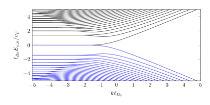
Figure 1: Particle-hole-symmetric energy spectrum for a graphene fold in a magnetic field. The bulk modes have a flat dispersion whereas the edge-modes we have $|dE/dk|\lesssim v_{F}$.

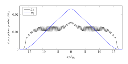
Figure 2: Absorption probability into the boundary modes for photons with polarization perpendicular and parallel to the fold. The values do not exceed the absorption of free graphene, $g_{\mathrm{free}}=\pi\alpha$. The absorption probability vanishes when the distance between the absorbed photon and the edge exceeds the classical cyclotron radius of the charge carriers.

In terms of the eigenfunctions, one can evaluate the Green functions and subsequently the optical conductivities (10). Employing the particle-hole-symmetry and the pseudo-parity, we obtain at zero temperature for each spin degree of freedom

$$\sigma_{\perp,\parallel}(x,\Omega)=\frac{(qv_{F})^{2}}{4\Omega}\int dk\sum_{m,l=1}^{\infty}\delta(\Omega-E_{m,k}-E_{l,k})$$

$$\times\left[1+\lambda_{\perp,\parallel}(-1)^{l+m}\right]\int dx^{\prime}\psi^{K}_{A,k,m}(-x^{\prime})\psi^{K}_{A,k,l}(x^{\prime})$$

$$\times\psi^{K}_{A,k,m}(-x)\psi^{K}_{A,k,l}(x)+(K\rightarrow K^{\prime})\,.$$ (20)

Here we have $\lambda_{\perp}=1$ ($\lambda_{\parallel}=-1$) for the conductance perpendicular (parallel) to the fold. We infer from (III.1) that the conductivity perpendicular to the fold involves only transitions between states of equal pseudo-parity and the states with opposite pseudo-parity define the conductivity parallel to the edge.

The absorption probability $g$ is the ratio of absorbed energy flux, $W_{\mathrm{abs}}=\sum_{i}J_{i}E_{i}$ and incident energy flux $W_{\mathrm{inc}}=\sum_{i}E_{i}E_{i}/(4\pi)$. Summing over the spin degrees of freedom gives then the relation between conductivity and absorption probability, $g_{\perp,\parallel}(x,\Omega)=8\pi\sigma_{\perp,\parallel}(x,\Omega)$.

The polarization- and distance dependent absorption probability into the dispersive edge channels is depicted in Fig. 2. We choose the photon energy to be $\Omega=17v_{F}/\ell_{B_{0}}$ at a magnetic field strength of $B=5T$ which corresponds to a photon energy of $\Omega=1$eV. In a semiclassical picture, a generated electron-hole pair would then propagate on circular trajectories with radius $r_{\mathrm{cyc}}=(\Omega/2)\ell^{2}_{B_{0}}/v_{F}=8.5\ell_{B_{0}}$ Keeping this in mind, we can interpret the qualitative behavior of the $g_{\perp}$ and $g_{\parallel}$. For a photon which is polarized perpendicular to the fold, the transition matrix elements are proportional to the momentum component $k_{\parallel}$, i.e. $\bar{\Psi}_{E}\gamma^{1}\Psi_{-E}\propto k_{\parallel}/\sqrt{k_{\parallel}^{2}+k_{\perp}^{2}}$. Thus, as shown in the left panel of Fig. 3, the charge carriers tend to propagate parallel to the fold before the magnetic field forces them on circular trajectories. As consequence, many of the trajectories will intersect with the graphene fold if the particle-hole pair is generated at a distance $x\lesssim 2r_{\mathrm{cyc}}$. This explains the rather sudden increase of $g_{\perp}(x)$ in Fig. 2. In contrast, an absorbed photon being polarized parallel to the fold is likely to generate particle-hole pairs propagating perpendicular to the fold before their trajectories are bend by the magnetic field, $\bar{\Psi}_{E}\gamma^{2}\Psi_{-E}\propto k_{\perp}/\sqrt{k_{\parallel}^{2}+k_{\perp}^{2}}$. From the right panel in Fig. 3 we infer that it is rather unlikely that charge carriers are reflected from the fold if they are generated at a distance $x\lesssim 2r_{\mathrm{cyc}}$. This in turn explains the gradual increase of $g_{\parallel}(x)$ towards the fold in Fig. 2.

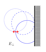
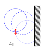
Figure 3: Left side: Perpendicular polarized photons generate particle-hole pairs which are propagating on circular trajectories. Most likely is the propagation on the solid circle whereas the trajectories of the dashed and dotted circles are less probable. We conclude that for this polarization most of the generated particle-hole pairs will be reflected at the graphene edge for distances $\lesssim 2r_{\mathrm{cyc}}$, cf. $g_{\perp}$ in Fig. 2. Right side: The same argument shows that for parallel polarized photons which are absorbed at a distance $\sim 2r_{\mathrm{cyc}}$ from the edge, the reflection of the generated charge-carriers at the edge is unlikely. A significant absorption can only be expected when the photon is absorbed at a distance $\sim r_{\mathrm{cyc}}$ to the edge which explains the gradual increase of $g_{\parallel}$ in Fig. 2.

III.2 Zigzag boundary

As noted before, the coordinate system for the tight-binding equations (1) and (2) was selected such that a zigzag boundary is parallel to the $x$-axis. Therefore we take the non-vanishing component of the vector potential to be in $x$-direction, $A_{x}(y)=-B_{0}y$. As in the fold-geometry, the two Dirac points can be treated separately. After decoupling the Dirac equations (5) and (6) one obtains the effective Schrödinger equations

$$[-\partial_{y}^{2}+(k-q\,B_{0}y)^{2}+qB_{0}]\psi^{K}_{A,k,m}=\frac{E_{m,k}^{2}}{v_{F}^{2}}\psi^{K}_{A,k,m}$$ (21)

and

$$[-\partial_{y}^{2}+(k-q\,B_{0}y)^{2}-qB_{0}]\psi^{K^{\prime}}_{A,k,m}=\frac{{E^{{}^{\prime}2}_{m,k}}}{v_{F}^{2}}\psi^{K^{\prime}}_{A,k,m}\,.$$ (22)

As the graphene sheet possesses a zigzag boundary, we can choose $A$-sublattice. Therefore the boundary condition translates to $\psi^{K}_{A,k,m}(y=0)=\psi^{K^{\prime}}_{A,k,m}(y=0)$=0. The energy bands are shown in Fig. 4 and the corresponding eigenfunctions can be expressed in terms of parabolic cylinder functions [30, 31]. Around the $K$-point there exists a zero-energy mode with one vanishing spinor component, $\psi^{K}_{A,k,0}(y)=0$ and $\psi^{K}_{B,k,0}(y)\sim\exp[-(qB_{0}y-k)^{2}/(2qB_{0})]$. Decomposing the Dirac spinor into eigenmodes which are labelled by the parallel momentum, the Landau band and the Dirac point, we obtain

$$\hat{\Psi}(\mathbf{r},t)=\frac{1}{2\pi\sqrt{2}}\int d{k}\sum_{m=0}e^{ikx}$$

$$\Bigg{[}\begin{pmatrix}0\\ \Psi^{\mathfrak{p},K^{\prime}}_{k,m}(y)\end{pmatrix}\hat{a}^{K^{\prime}}_{m,k}e^{-iE^{K^{\prime}}_{m,k}t}+\begin{pmatrix}0\\ \Psi^{\mathfrak{h},K^{\prime}}_{k,m}(y)\end{pmatrix}\hat{b}^{\dagger K^{\prime}}_{m,k}e^{+iE^{K^{\prime}}_{m,k}t}\Bigg{]}$$

$$+\frac{1}{2\pi\sqrt{2}}\int d{k}\sum_{m>0}e^{ikx}$$

$$\Bigg{[}\begin{pmatrix}\Psi^{\mathfrak{p},K}_{k,m}(y)\\ 0\end{pmatrix}\hat{a}^{K}_{m,k}e^{-iE^{K}_{m,k}t}+\begin{pmatrix}\Psi^{\mathfrak{h},K}_{k,m}(y)\\ 0\end{pmatrix}\hat{b}^{\dagger K}_{m,k}e^{+iE^{K}_{m,k}t}\Bigg{]}$$

$$+\frac{1}{2\pi}\int d{k}\,e^{ikx}\begin{pmatrix}\Psi^{K}_{k,0}(y)\\ 0\end{pmatrix}\hat{a}^{K}_{0,k}$$ (23)

The components of $\Psi^{\mathfrak{h},K,K^{\prime}}_{k,m}(y)$ and $\Psi^{\mathfrak{p},K,K^{\prime}}_{k,m}(y)$ can taken to be real (cf. Eqs. (5). After some algebra we obtain for the conductance

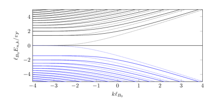
Figure 4: Energybands for a graphene sheet with zigzag edge in a magnetic field. The dotted curves correspond to the energybands for the modes in the vicinity of the $K^{\prime}$-point whereas the energybands for the second Dirac point $K$ are represented by solid lines. The boundary condition induces a zero energy mode at $K$.

$$\sigma_{\perp,\parallel}(y,\Omega)=\frac{(qv_{F})^{2}}{4\Omega}\int dk\int dy^{\prime}\sum_{l=1}^{\infty}$$

$$\times\bigg{[}\sum_{m=1}^{\infty}\delta(\Omega-E^{K}_{m,k}-E^{K}_{l,k})\psi^{K}_{A,k,l}(y^{\prime})\psi^{K}_{B,k,m}(y^{\prime})$$

$$\times[\psi^{K}_{A,k,l}(y)\psi^{K}_{B,k,m}(y)+\lambda_{\perp,\parallel}\psi^{K}_{A,k,m}(y)\psi^{K}_{B,k,l}(y)]$$

$$+\delta(\Omega-E^{K}_{l,k})\psi^{K}_{A,k,l}(y^{\prime})\psi^{K}_{B,k,0}(y^{\prime})\psi^{K}_{A,k,l}(y)\psi^{K}_{B,k,0}(y)\bigg{]}$$

$$+ \frac{(qv_{F})^{2}}{4\Omega}\int dk\int dy^{\prime}\sum_{l,m=0}^{\infty}$$

$$\times\bigg{[}\delta(\Omega-E^{K^{\prime}}_{m,k}-E^{K^{\prime}}_{l,k})\psi^{K^{\prime}}_{A,k,l}(y^{\prime})\psi^{K^{\prime}}_{B,k,m}(y^{\prime})$$

$$\times[\psi^{K^{\prime}}_{A,k,l}(y)\psi^{K^{\prime}}_{B,k,m}(y)+\lambda_{\perp,\parallel}\psi^{K^{\prime}}_{A,k,m}(y)\psi^{K^{\prime}}_{B,k,l}(y)]$$ (24)

As for the fold geometry, cf. (III.1), the conductivity is determined by the generation of particle-hole pairs at $K$ and $K^{\prime}$. However, for the zigzag boundary, the excitations around the Dirac points contribute differently to the absorption probability. In particular the presence of the zero energy mode at the Dirac point $K$ permits the absorption of the photon energy into a single particle- or hole excitation, see equation (III.2). This contribution is independent of the polarization. The qualitative behavior of the absorption probabilities $g_{\perp}$ and $g_{\parallel}$ can be justified with the same arguments as before.

From Figs. (2) and (5) we infer that the maximum absorption probability into the edge modes does not exceed the absorption of monolayer graphene, $g_{0}=\pi\alpha_{\mathrm{QED}}$. Note that we selected $\Omega$ to be off-resonant such that the absorption into the bulk modes did not contribute. Alltogether we conclude that the large current observed in [14] cannot be traced back to an enhanced absorption. As possible explanation for this effect we shall consider estimates for charge carrier multiplication rates due to impact ionization.

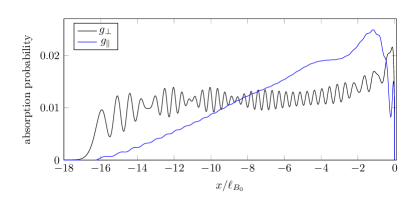
Figure 5: Absorption probability into the dispersive edge modes for the polarizations perpendicular and parallel to the zigzag edge. The curves show the same qualitative behavior as the absorption probabilities around a graphene fold. The peaks in the vicinity of $x=0$ are mainly due to the presence of the zero energy mode.

IV Secondary particle-hole pair creation

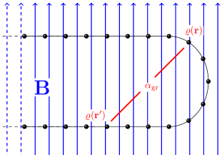
Figure 6: Sketch of the graphene fold in an external magnetic field. Secondary particle-hole pairs are generated via the Coulomb interaction.

Auger processes have been studied thoroughly for translational invariant graphene sheets [32, 33, 34, 35]. The energy-momentum conservation together with the linear dispersion relation restricts the phase space for interactions to one dimension, i.e. only collinear processes are allowed [32]. In contrast, a graphene edge breaks the translational invariance and opens up a finite phase-space volume for carrier multiplication.

Our analysis will reside on the bare Coulomb Hamiltonian

$$\hat{H}_{\mathrm{Coulomb}}=\frac{q^{2}}{2}\int d^{2}r\int d^{2}{r^{\prime}}\frac{\hat{\varrho}(\mathbf{r})\hat{\varrho}(\mathbf{r}^{\prime})}{4\pi\epsilon_{0}|\mathbf{r}-\mathbf{r}^{\prime}|}\,,$$ (25)

where the electron densities can be written in terms of the Dirac fields as

$$\hat{\varrho}(\mathbf{r})=\sum_{\sigma}\left(\big{[}\hat{\Psi}_{\sigma}^{K}(\mathbf{r})\big{]}^{\dagger}\hat{\Psi}_{\sigma}^{K}(\mathbf{r})+\big{[}\hat{\Psi}_{\sigma}^{K^{\prime}}(\mathbf{r})\big{]}^{\dagger}\hat{\Psi}_{\sigma}^{K^{\prime}}(\mathbf{r})\right)\,.$$ (26)

Here we employed the expressions (3) and (4) and neglected rapidly oscillating terms $\sim e^{i(\mathbf{K}-\mathbf{K}^{\prime})\cdot\mathbf{r}}$. The label $\sigma$ denotes the spin degree of freedom which was suppressed in the previous sections.

We emphasize that our study is solely based on Fermi’s Golden rule. Our analysis for carrier multiplication around the graphene edge shall give only a rough order-of-magnitude estimate for the charge carrier multiplication whereas the actual scattering rates are likely to be smaller. In fact, the dielectric constant will be diminished due to the substrate material or electronic screening [36, 37]. However, as consequence of the vanishing density of states, electronic screening at the Dirac point is rather inefficient [36].

We consider Auger-type inelastic scattering of an incoming electron, $|\mathrm{in}\rangle=|k_{\mathrm{in}},n_{\mathrm{in}}\rangle$, to an outgoing electron, $|\mathrm{out}\rangle=|k_{\mathrm{out}},n_{\mathrm{out}}\rangle$, while creating an electron-hole pair $|\mathrm{part},\mathrm{hole}\rangle=|k_{\mathrm{part}},n_{\mathrm{part}},k_{\mathrm{hole}},n_{\mathrm{hole}}\rangle$. Using standard first order perturbation theory, we find for the transition matrix elements

$$M(\mathrm{in}\rightarrow\mathrm{out},\mathrm{part},\mathrm{hole})\\ =-i\int dt\langle\mathrm{out},\mathrm{part},\mathrm{hole}|\hat{H}_{\mathrm{Coulomb}}|\mathrm{in}\rangle\,.$$ (27)

Summing the absolute square of (27) over all final states gives the leading order result for the impact ionization rate. If we assume, that the momentum of the incoming particle is in the vicinity of the Dirac point $K$ and the secondary particle-hole pair is generated around $K^{\prime}$, the probability per unit time reads

$$\frac{\mathcal{P}^{K,\sigma\rightarrow K^{\prime},\lambda}}{T}=\frac{v_{F}\,\alpha_{\mathrm{graphene}}^{2}}{8\pi}\int dk_{\mathrm{out}}\mathcal{H}^{K,\sigma\rightarrow K^{\prime},\lambda}(k_{\mathrm{out}})$$ (28)

where the integrand

$$\mathcal{H}^{K,\sigma\rightarrow K^{\prime},\lambda}(k_{\mathrm{out}})=\frac{v_{F}}{|\frac{d\mathcal{F}}{dk_{\mathrm{part}}}|}\left|\mathcal{I}^{K,\sigma\rightarrow K^{\prime},\lambda}\right|^{2}\bigg{|}_{\mathcal{F}=0}$$ (29)

is determined by an overlap integral specifying the Coulomb interaction between charge densities,

$$\mathcal{I}^{K,\sigma\rightarrow K^{\prime},\lambda}=\int dx\int dx^{\prime}\left[\Psi^{\mathfrak{p},K^{\prime}}_{k_{\mathrm{part}},n_{\mathrm{part}}}(x)\right]^{\dagger}\Psi^{\mathfrak{h},K^{\prime}}_{k_{\mathrm{hole}},n_{\mathrm{hole}}}(x)$$

$$\times K_{0}\left(|k_{\mathrm{in}}-k_{\mathrm{out}}|D(x,x^{\prime})\right)\left[\Psi^{\mathfrak{p},K}_{k_{\mathrm{out}},n_{\mathrm{out}}}(x^{\prime})\right]^{\dagger}\Psi^{\mathfrak{p},K}_{k_{\mathrm{in}},n_{\mathrm{in}}}(x^{\prime})$$ (30)

and a weight factor $d\mathcal{F}/dk_{\mathrm{part}}$, see below. The modified Bessel function of second kind $K_{0}$ in (IV) arises from integrating out the direction parallel to the edge. Its argument contains the momentum difference between incoming and outgoing particle and the function $D(x,x^{\prime})$ that measures the distance of the charge densities perpendicular to the fold. Two variables can be eliminated using the momentum conservation, $k_{\mathrm{in}}-k_{\mathrm{out}}=k_{\mathrm{part}}-k_{\mathrm{hole}}$, and the energy conservation, $\mathcal{F}=E_{n_{\mathrm{in}},k_{\mathrm{in}}}-E_{n_{\mathrm{out}},k_{\mathrm{out}}}-E_{n_{\mathrm{part}},k_{\mathrm{part}}}-E_{n_{\mathrm{hole}},k_{\mathrm{hole}}}\equiv 0$. The weight factor $d\mathcal{F}/dk_{\mathrm{part}}$ in (28) ensures the local reparametrization invariance of the integral. The reparametrization invariance for the whole integration domain does not exists in general since $dk_{\mathrm{out}}/dk_{\mathrm{part}}$ can become singular due to energy-momentum conservation. Nevertheless, it is always possible to find a parametrization for $\mathcal{H}$ which governs the complete integration domain.

The matrix-elements for impact ionization in the same Dirac valley but opposite spin are analogous to (28) with $K^{\prime}\rightarrow K$ or $K\rightarrow K^{\prime}$. In contrast, when the spin and the valley index are the same, the outgoing electron is indistinguishable from the generated particle. Therefore the probability $\mathcal{P}^{K,\sigma\rightarrow K,\sigma}$ is now determined by overlap integrals which satisfy an exchange symmetry,

$$\mathcal{I}^{K,\sigma\rightarrow K,\sigma}=\int dx\int dx^{\prime}\left[\Psi^{\mathfrak{p},K}_{k_{\mathrm{part}},n_{\mathrm{part}}}(x)\right]^{\dagger}\Psi^{\mathfrak{h},K}_{k_{\mathrm{hole}},n_{\mathrm{hole}}}(x)$$

$$\times K_{0}\left(|k_{\mathrm{in}}-k_{\mathrm{out}}|D(x,x^{\prime})\right)\left[\Psi^{\mathfrak{p},K}_{k_{\mathrm{out}},n_{\mathrm{out}}}(x^{\prime})\right]^{\dagger}\Psi^{\mathfrak{p},K}_{k_{\mathrm{in}},n_{\mathrm{in}}}(x^{\prime})$$

$$-(k_{\mathrm{out}},n_{\mathrm{out}}\leftrightarrow k_{\mathrm{part}},n_{\mathrm{part}})\,.$$ (31)

Before we discuss the specific settings of a graphene fold and a zigzag boundary, two remarks are in order. First, the leading-order perturbation theory may not be very accurate since the dimensionless expansion parameter is larger than unity, $\alpha_{\mathrm{graphene}}=\alpha_{\mathrm{QED}}{c}/{v_{F}}\approx 2.2$. Second, we will not consider Auger recombination and assume that the generated charge carriers reach the bond contacts of the graphene boundary before particle-hole annihilation occurs. Particle-hole annihilation can in principal be considered within a Boltzmann-equation approach [32]. However, we expect the recombination rates to be negligible for sufficiently small electron-hole densities, see also [38].

IV.1 Graphene fold

A graphene fold breaks translational invariance without terminating the graphene sheet. As in section III.1, we assume that the magnetic length $\ell_{\mathrm{B}}$ and the fold radius $R$ to be equal. The spatial separation $D(x,x^{\prime})$ of the charge carrier densities can be deduced by simple geometric considerations from Fig. 6.

An exact selection rule occurs due to the pseudo parity which was briefly discussed in section III.1. As consequence, the integrals $\mathcal{I}^{K,\sigma\rightarrow K,\lambda}$ and $\mathcal{I}^{K,\sigma\rightarrow K^{\prime},\lambda}$ vanish identically unless the sum of the Landau level indices, $n_{\mathrm{in}}+n_{\mathrm{out}}+n_{\mathrm{part}}+n_{\mathrm{hole}}$, equals an odd integer. From the allowed transitions, only a few decay channels dominate the process, whereas most of the channels will be suppressed by several orders of magnitude. If the number of nodes of the wavefunctions $\Psi^{\mathfrak{p},K}_{k_{\mathrm{in}},n_{\mathrm{in}}}$ and $\Psi^{\mathfrak{p},K}_{k_{\mathrm{out}},n_{\mathrm{out}}}$ are very different from each other, the wave functions are nearly orthogonal which renders the overlap integral (IV) exponentially small. The same is true for $\Psi^{\mathfrak{p},K^{\prime}}_{k_{\mathrm{part}},n_{\mathrm{part}}}$ and $\Psi^{\mathfrak{p},K^{\prime}}_{k_{\mathrm{hole}},n_{\mathrm{hole}}}$. Therefore, the decay channels between the Dirac points $K$ and $K^{\prime}$ can usually be neglected unless $n_{\mathrm{part}}\sim n_{\mathrm{hole}}$ and $n_{\mathrm{in}}\sim n_{\mathrm{out}}$.

Furthermore, a strong oscillation of the integrands will render the overlap integrals exponentially small. In order to keep the total number of nodes of the integrand in equation (IV) as small as possible, we can conclude that for an incoming particle at Landau level $n_{\mathrm{in}}$ the following approximate selection rule applies:

$$n_{\mathrm{out}}\in\{n_{\mathrm{in}},n_{\mathrm{in}}\pm 1\}\text{ and }n_{\mathrm{part}}\sim n_{\mathrm{hole}}\sim 1\,.$$ (32)

For transitions within the same Dirac point, we obtain also relevant contributions for $n_{\mathrm{out}}\sim n_{\mathrm{hole}}\gg n_{\mathrm{in}}\sim n_{\mathrm{part}}$, a direct consequence of the exchange symmetry, see equation (IV).

We illustrate our findings and consider the decay process of an incoming particle with $n_{\mathrm{in}}=5$ and $k_{\mathrm{in}}=10/\ell_{B_{0}}$. Assuming a magnetic field $B_{0}=5T$, this would correspond to an initial energy of $E_{n_{\mathrm{in}},k_{\mathrm{in}}}=0.7$ eV. For transitions involving states of both Dirac points, we listed the rates for various decay channels in Table 1. Although the applicability of first order perturbation theory should be doubted and not every generated charge carrier will contribute to the overall current, see below, we see from Table 1 that each of the largest decay channels generates between 80 and 90 particle-hole pairs within one picosecond which is about 10 particle-hole pairs within the distance of a classical cyclotron radius.

Fig. 7 shows the magnitude of the integrals which determine the decay channels $\mathcal{P}^{K,\sigma\rightarrow K^{\prime},\lambda}(n_{\mathrm{in}}\rightarrow n_{\mathrm{out}},n_{\mathrm{part}},n_{\mathrm{hole}})$. Transitions which do not fulfill the relation (32) are strongly suppressed in comparison with the dominating decay channels.

$n_{\mathrm{out}}$	$n_{\mathrm{part}}$	$n_{\mathrm{hole}}$	$\mathcal{P}/T$ in s-1
4	1	1	$9.4\cdot 10^{13}$
6	1	1	$8.1\cdot 10^{13}$
1	4	1	$1.5\cdot 10^{12}$
1	6	1	$4.5\cdot 10^{11}$

Table 1: The first two rows specify the largest decay rates for transitions $K\rightarrow K^{\prime}$ for an incoming particle with $n_{\mathrm{in}}=5$ and $k_{\mathrm{in}}~{}=~{}10/\ell_{B_{0}}$. The decay rates in the third and fourth line are at least one magnitude smaller since they do not fulfill (32).

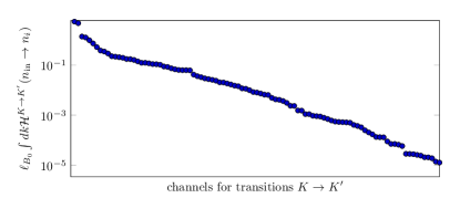
Figure 7: Overlap integrals which determine the decay probabilities per unit time. Here we only consider the channels for which the incoming particle is in the vicinity of the $K$-point and the outgoing particle-hole pair in generated around the $K^{\prime}$-point. The corresponding rates for the two largest integrals are listed in Table 1. As can be seen here, the remaining channels are strongly suppressed.

For transitions in the vicinity of one Dirac point, we listed the dominating integrals in Table 2. Here, all rates come in pairs which is a direct consequence of the exchange symmetry of (IV), from which follows that $\mathcal{P}^{K,\sigma\rightarrow K,\sigma}(n_{\mathrm{out}},n_{\mathrm{part}})=\mathcal{P}^{K,\sigma\rightarrow K,\sigma}(n_{\mathrm{part}},n_{\mathrm{out}})$. Comparing the corresponding rates of Table 1 and 2 we find $\mathcal{P}^{K,\sigma\rightarrow K,\sigma}\lesssim\mathcal{P}^{K,\sigma\rightarrow K^{\prime},\sigma}$. This small suppression in comparison to the $K\rightarrow K^{\prime}$-rates originates from destructive interference which are rather small unless $n_{\mathrm{out}}\sim n_{\mathrm{part}}$, cf. equations (32) and (IV). In Fig. 8, we show the matrix elements determing the $K\rightarrow K$-transitions sorted by size.

$n_{\mathrm{out}}$	$n_{\mathrm{part}}$	$n_{\mathrm{hole}}$	$\mathcal{P}/T$ in $s^{-1}$
4	1	1	$8.3\cdot 10^{13}$
1	4	1	$8.3\cdot 10^{13}$
6	1	1	$7.5\cdot 10^{13}$
1	6	1	$7.5\cdot 10^{13}$

Table 2: Decay rates of the dominating channels for an incoming particle with $n_{\mathrm{in}}=5$ and $k_{\mathrm{in}}=10/\ell_{B_{0}}$. The rates are symmetric w.r.t the interchange of $n_{\mathrm{out}}$ and $n_{\mathrm{part}}$.

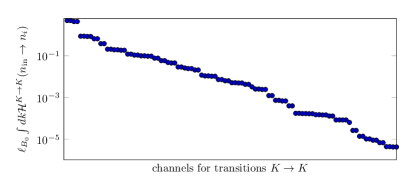
Figure 8: Overlap integrals determining the decay probabilities per unit time in the vicinity of one Dirac point time sorted by size on a logarithmic scale. As consequence of the exchange symmetry, all matrix elements occur in pairs.

Summing over the spin configurations, both Dirac points and all final configurations for the outgoing particle and the generated particle-hole pair, we find for our example the total impact ionization rate

$$\frac{\mathcal{P}_{\mathrm{total}}}{T} =\frac{1}{T}\sum_{\lambda}\sum_{n_{\mathrm{I}}}\left(3\mathcal{P}_{\mathrm{n_{I}}}^{K,\sigma\rightarrow K^{\prime},\lambda}+\mathcal{P}_{\mathrm{n_{I}}}^{K,\sigma\rightarrow K,\lambda}\right)$$

$$\approx 1.4\cdot 10^{15}\mathrm{s}^{-1}$$ (33)

which corresponds to about 180 generated particle-hole pairs within a distance of one cyclotron radius. Although some of the secondary particles and holes are generated in the bulk and do not contribute to the total current, see below, our estimate shows the efficiency of the charge carrier multiplication.

In our example, one of the dominating channels in the pair production process with transitions $K\rightarrow K$ is specified by the quantum numbers $n_{\mathrm{in}}=5$, $n_{\mathrm{out}}=1$, $n_{\mathrm{part}}=4$ and $n_{\mathrm{hole}}=1$. The corresponding integrand $\mathcal{H}^{K,\sigma\rightarrow K,\sigma}$ for this decay channel is shown in the upper panel of Fig. 9. In the lower panel in Fig. 9 we see the currents $J=dE/dk$ for the outgoing particle and the generated particle hole-pair. For $k_{\mathrm{out}}\lesssim-1.5/l_{B_{0}}$, the whole energy of the incoming particle is transferred to the generated particle whereas the generated hole and the outgoing particle are bulk modes with zero energy. In contrast, for $k_{\mathrm{out}}\gtrsim-1.5/l_{B_{0}}$, the outgoing particle and the generated hole are located in the vicinity of the boundary and additional current is generated.

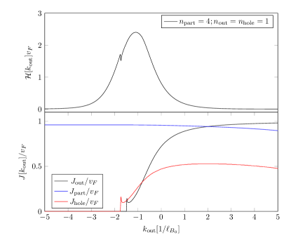
Figure 9: Upper panel: Value of $\mathcal{H}^{K,\sigma\rightarrow K,\sigma}$ as function of $k_{\mathrm{out}}$. Lower panel: Currents related to the outgoing particle and the generated particle-hole pair. The cusps in the plots around $k_{\mathrm{out}}=-1.5/l_{B_{0}}$ originate from the slope of the lowest energy band in our model, cf. Fig. 1.

In our example, the function $\mathcal{H}^{K,\sigma\rightarrow K,\sigma}$ has its maximum around $k_{\mathrm{out}}\ell_{B_{0}}\sim-1$. In general, the position of this maximum determines the contribution of the generated charge carriers to the overall current. To clarify this statement and its consequence, we consider a general transition with $n_{\mathrm{part}}=n_{\mathrm{in}}-1$ and $\ell_{B_{0}}k_{\mathrm{in}}\gg 1$ and $n_{\mathrm{out}}=n_{\mathrm{hole}}=1$. The Coulomb integral (IV) is exponentially suppressed unless $\ell_{B_{0}}(k_{\mathrm{in}}-k_{\mathrm{part}})\ll 1$. Together with (14) and the energy conservation we infer that the energies of the outgoing particle and the generated hole are small,

$$\left(E_{n_{\mathrm{out}},k_{\mathrm{out}}}+E_{n_{\mathrm{hole}},k_{\mathrm{hole}}}\right)\\ =\frac{v_{F}}{\ell_{B_{0}}}\mathcal{O}\left\{\ell_{B_{0}}(k_{\mathrm{in}}-k_{\mathrm{part}}),1/\sqrt{\ell_{B_{0}}k_{\mathrm{in}}}\right\}\,.$$ (34)

Thus, the outgoing particle and the generated hole will be either zero energy modes of the form (15) or low energy modes at the boundary, see equation (19).

If $n_{\mathrm{in}}\sim 1$ and $\ell_{B_{0}}k_{\mathrm{in}}\gg 1$ we know from (14) that $\Psi_{{k_{\mathrm{in}}},{n_{\mathrm{in}}}}^{\mathfrak{p},K}$ and $\Psi_{{k_{\mathrm{part}}},{n_{\mathrm{part}}}}^{\mathfrak{p},K}$ are located around the edge and therefore $\mathcal{H}^{K,\sigma\rightarrow K,\sigma}$ will adopt its maximum value at $|k_{\mathrm{out}}|\ell_{B_{0}}\lesssim 1$ if the wavefunctions $\Psi_{{k_{\mathrm{out}}},{n_{\mathrm{out}}}}^{\mathfrak{p},K}$ and $\Psi_{{k_{\mathrm{hole}}},{n_{\mathrm{hole}}}}^{\mathfrak{h},K}$ are both dispersive edge modes of the form (19). In contrast, for $n_{\mathrm{in}}\gg 1$ the greatest weight of the wave functions $\Psi_{{k_{\mathrm{in}}},{n_{\mathrm{in}}}}^{\mathfrak{p},K}$ and $\Psi_{{k_{\mathrm{part}}},{n_{\mathrm{part}}}}^{\mathfrak{p},K}$ are close to the classical turning points inside the bulk,

$$\frac{|x_{\mathrm{turn}}|}{\ell_{B_{0}}}\approx\frac{\sqrt{2n_{\mathrm{in}}}}{\left(\ell_{B_{0}}k_{\mathrm{in}}\right)^{1/4}}\,.$$ (35)

Here $\mathcal{H}^{K,\sigma\rightarrow K,\sigma}$ adopts its maximum value if the outgoing particle and the generated hole are bulk modes. The position of the maximum of $\mathcal{H}^{K,\sigma\rightarrow K,\sigma}$ can be estimated from (15) and (35) to be at $\ell_{B_{0}}k_{\mathrm{out}}\approx-\sqrt{2n_{\mathrm{in}}}/\left(\ell_{B_{0}}k_{\mathrm{in}}\right)^{1/4}$.

In total, we conclude that initial states with small $n_{\mathrm{in}}$ are beneficial for the current enhancement. For these dispersive edge modes we have $n_{\mathrm{in}}/k_{\mathrm{in}}\ell_{B_{0}}\ll 1$ which corresponds to charge excitations traveling nearly parallel to the fold. In contrast, for large $n_{\mathrm{in}}$ only the final states which are inside the tail of $\mathcal{H}^{K\rightarrow K}$ at $|\ell_{B_{0}}k_{\mathrm{out}}|\lesssim 1$ are relevant for the generated current.

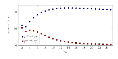
Figure 10: We consider the decay channels from an incoming electron at Landau band $n_{\mathrm{in}}$ with an initial energy $E_{n_{\mathrm{in}},k_{\mathrm{in}}}=0.7$ eV to the outgoing states which are specified by $n_{\mathrm{in}}\rightarrow n_{\mathrm{out}}=n_{\mathrm{in}}-1$ and $n_{\mathrm{part}}=n_{\mathrm{hole}}=1$. The blue dots denote the generation rates for particle-hole pairs whereas the red squares are the corresponding rates for additionally generated charge carriers which contribute to the edge current.

In order to quantify our statement, we calculated the expectation value of the sum of all currents $J_{k}=dE/dk$ i.e

$$\frac{\mathcal{C}^{K,\sigma\rightarrow K,\sigma}}{T}=\frac{\alpha^{2}_{\mathrm{graphene}}}{8\pi}\\ \times\int dk_{\mathrm{out}}\left(J_{k_{\mathrm{out}}}+J_{k_{\mathrm{part}}}+J_{k_{\mathrm{hole}}}-J_{k_{\mathrm{in}}}\right)\mathcal{H}^{K,\sigma\rightarrow K,\sigma}$$ (36)

This quantity can be interpreted as generated particles per unit time which contribute to the edge current. From Fig. 10 we conclude that, although the number of generated charge carriers grows with increasing $n_{\mathrm{in}}$, the generation of edge modes adopts its maximum value at small values of $n_{\mathrm{in}}$. Going back to our initial example we find after summing over all final states $\mathcal{C}_{\mathrm{total}}/T\approx 7.8\cdot 10^{14}$s^-1. Comparing with (IV.1) we conclude that only every fourth generated charge carrier will contribute to the edge current.

IV.2 Zigzag boundary

The carrier multiplication process is a rather robust effect and we expect that the main characteristics of the decay process also holds for a graphene sheet with zigzag boundary.

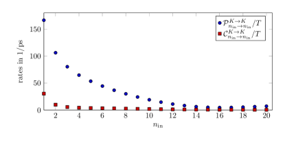
Figure 11: Transitions within the Dirac point $K$ are dominated by channels that contain the zero energy mode.

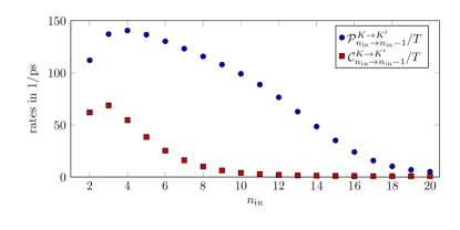
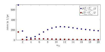
Figure 12: Upper panel: Rates for the transitions between the two Dirac points. The quantum numbers for the incoming and outgoing electron are $n_{\mathrm{in}}$ and $n_{\mathrm{out}}=n_{\mathrm{in}}-1$ and the particle-hole pair is generated in the state with $n_{\mathrm{part}}=n_{\mathrm{hole}}=0$. The magnitude of these rates are comparable with the results we found in the graphene fold, see Fig. 10. Lower panel: Rates for channels which are specified by $n_{\mathrm{in}}=n_{\mathrm{out}}$ and $n_{\mathrm{part}}=n_{\mathrm{hole}}=0$ are dominating the Auger process for small values of $n_{\mathrm{in}}$.

As for the fold geometry, we find that the overlap integrals $\mathcal{I}^{K,\sigma\rightarrow K,\lambda}$ and $\mathcal{I}^{K,\sigma\rightarrow K^{\prime},\lambda}$ are strongly suppressed unless the approximate selection rule (32) applies. Therefore, as for the fold geometry, the charge carrier multiplication is dominated by a few channels.

We assumed for the incoming electron the same energy as before, i.e. $E_{n_{\mathrm{in}},k_{\mathrm{in}}}=0.7$ eV. The dominant transitions $K\rightarrow K$ contain a zero energy mode $\psi^{K}_{0,k}$ with one vanishing spinor component, see equation (III.2). The presence of this non-dispersive enlarges the phase-space for these channels since momentum-conservation can always be satisfied. In Fig. 11 we show the probabilities per unit time $\mathcal{P}^{K,\sigma\rightarrow K,\sigma^{\prime}}/T$ for the processes involving the zero energy mode and $n_{\mathrm{in}}=n_{\mathrm{out}}$ as well as $n_{\mathrm{hole}}=1$. For increasing $n_{\mathrm{in}}$, the weight of the corresponding wavefunction is moving inside the bulk which diminishes the overlap with the particle-hole modes at the boundary. As before, this implies that small values of $n_{\mathrm{in}}$ are beneficial for the current enhancement.

We found also rather large rates for transitions between both graphene valleys, $K\rightarrow K^{\prime}$. Transitions with $n_{\mathrm{out}}=n_{\mathrm{in}}-1$ and $n_{\mathrm{part}}=n_{\mathrm{hole}}=0$ are presented in upper panel of Fig. 12 and are of similar magnitude as the rates in the graphene fold, cf. Fig. 10. The largest contribution to the impact ionization originates from transitions with the quantum numbers $n_{\mathrm{in}}=n_{\mathrm{out}}=1$ and $n_{\mathrm{part}}=n_{\mathrm{hole}}=0$, see the lower panel of Fig. 12. Note that these transitions are absent in the graphene fold due to the pseudo-parity selection rule.

V Conclusions and Outlook

We analyzed the primary magneto-optical absorption of graphene and the subsequent particle-hole generation due to impact ionization. The bare magneto-photoelectric, in particular the absorption into the dispersive edge modes, does not exceed the well-known value for graphene monolayers. However, subsequent impact ionization leads to charge carrier multiplication and therefore to a strong enhancement of the photo-current. We found that charge carrier multiplication depends on the incident angle between incoming electron and graphene edge, particularly small impact angles are advantageous for current amplification. The presence of a finite phase space volume due to absence of translational invariance makes this effect rather robust. However, the specific enhancement will depend on the particular boundary condition of the graphene edge.

Our findings are consistent with previous investigation on the magneto-photoelectric effect [14] and should be of relevance for possible future applications such as graphene-based photodetectors.

The derived exact and approximate selection rules show that only a small subset of the decay channels will significantly contribute to the dynamics. Using this results could permit the efficient implementation of the relaxation dynamics using a Boltzmann equation approach. Although we expect that the qualitative behavior of the charge multiplication can already be captured within leading order perturbation theory, a quantitative prediction should include higher order corrections of the scattering processes.

References

• [1] A. A. Balandin, S. Ghosh, W. Bao, I. Calizo, D. Teweldebrhan, F. Miao and C. N. Lau, Superior thermal conductivity of single-layer graphene, Nano Lett. 8, 902 (2008).
• [2] A. S. Mayorov, R. V. Gorbachev, S. V. Morozov, L. Britnell, R. Jalil, L. A. Ponomarenko, P. Blake, K. S. Novoselov, K. Watanabe, T. Taniguchi and A. K. Geim, Micrometer-Scale Ballistic Transport in Encapsulated Graphene at Room Temperature, Nano Lett. 11, 2396 (2011).
• [3] A. H. Castro Neto, F. Guinea, N. M. R. Peres, K. S. Novoselov and A. K. Geim, The electronic properties of graphene, Rev. Mod. Phys. 81, 109 (2009).
• [4] R. Nair, P. Blake, A. N. Grigorenko, K. S. Novoselov, T. J. Booth, T. Stauber, N. M. R. Peres and A. K. Geim, Fine Structure Constant Defines Visual Transparency of Graphene, Science, 320, 1308 (2008).
• [5] P. Ma, Y. Salamin, B. Baeuerle, A. Josten, W. Heni, A. Emboras and J. Leuthold, Plasmonically Enhanced Graphene Photodetector Featuring 100 Gbit/s Data Reception, High Responsivity, and Compact Size, ACS Photonics, 6, 154 (2019).
• [6] F. Bonaccorso, Z. Sun, T. Hasan and A. C. Ferrari, Graphene photonics and optoelectronics, Nature Photonics 4, 611 (2010).
• [7] F. H. L. Koppens, T. Mueller, Ph. Avouris, A. C. Ferrari, M. S. Vitiello and M. Polini, Photodetectors based on graphene, other two-dimensional materials and hybrid systems, Nature Nanotechnology 9, 780 (2014).
• [8] J. C. W. Song, M. S. Rudner, C. M. Marcus and L. S. Levitov, Hot Carrier Transport and Photocurrent Response in Graphene, Nano Lett. 11, 4688 (2011).
• [9] S. Candussio, M. V. Durnev, S. A. Tarasenko, J. Yin, J. Keil, Y. Yang, S.-K. Son, A. Mishchenko, H. Plank, V. V. Bel’kov, S. Slizovskiy, V. Fal’ko and S. D. Ganichev, Edge photocurrent driven by terahertz electric field in bilayer graphene, Phys. Rev. B 102, 045406 (2020).
• [10] Q. Ma, C. H. Lui, J. C. W. Song, Y. Lin, J. F. Kong, Y. Cao, T. H. Dinh, N. L. Nair, W. Fang, K. Watanabe, T. Taniguchi, S.-Y. Xu, J. Kong, T. Palacios, N. Gedik, N. M. Gabor and P. Jarillo-Herrero, Giant intrinsic photoresponse in pristine graphene, Nature Nanotechnology 14, 145 (2019).
• [11] M. Shimatani, S. Ogawa, D. Fujisawa, S. Okuda, Y. Kanai, T. Ono and K. Matsumoto, Photocurrent enhancement of graphene phototransistors using p–n junction formed by conventional photolithography process, Japanese Journal of Applied Physics, 55, 110307 (2016).
• [12] D. Sun, G. Aivazian, A. M. Jones, J. S. Ross, W. Yao, D. Cobden and X. Xu, Ultrafast hot-carrier-dominated photocurrent in graphene, Nature Nanotechnology 7, 114 (2012).
• [13] F. Queisser and R. Schützhold, Strong magnetophotoelectric effect in folded graphene, Phys. Rev. Lett. 111, 046601 (2013).
• [14] J. Sonntag, A. Kurzmann, M. Geller, F. Queisser, A. Lorke and R. Schützhold, Giant magneto-photoelectric effect in suspended graphene, New J. Phys., 19, 063028 (2017).
• [15] M. O. Goerbig, Electronic properties of graphene in a strong magnetic field, Rev. Mod. Phys. 83, 1193 (2011).
• [16] N. M. R. Peres and T. Stauber, Transport in a Clean Graphene Sheet at Finite Temperature and Frequency, Int. J. Mod. Phys. 22, 2536 (2008).
• [17] G. L. Klimchitskaya and V. M. Mostepanenko, Conductivity of pure graphene: Theoretical approach using the polarization tensor, Phys. Rev. B 93, 245419 (2019).
• [18] K. F. Mak, M. Y. Sfeir, Y. Wu, C. H. Lui, J. A. Misewich, and T. F. Heinz, Measurement of the Optical Conductivity of Graphene, Phys. Rev. Lett. 101, 196405 (2008).
• [19] K. J. Tielrooij, J. C. W. Song, S. A. Jensen, A. Centeno, A. Pesquera, A. Zurutuza Elorza, M. Bonn, L. S.Levitov and F. H. L. Koppens, Photoexcitation cascade and multiple hot-carrier generation in graphene, Nat. Phys. 9, 248 (2013).
• [20] T. Plötzing, T. Winzer, E. Malic, D. Neumaier, A. Knorr and H. Kurz, Experimental verification of carrier multiplication in graphene, Nano Lett. 14, 5371 (2014).
• [21] M. Mittendorff, F. Wendler, E. Malic, A. Knorr, M. Orlita, M. Potemski, C. Berger, W. A. de Herr, H. Schneider, M. Helm and S. Winnerl, Carrier dynamics in Landau-quantized graphene featuring strong Auger scattering Nat. Phys. 11, 75 (2015).
• [22] D. Brida, A. Tomadin, C. Manzoni, Y. J. Kim, A. Lombardo, S. Milana, R. R. Nair, K. S. Novoselov, A. C. Ferrari, G. Cerullo and M. Polini, Ultrafast collinear scattering and carrier multiplication in graphene, Nature Communications 4, 1987 (2013).
• [23] T. Ando, Theory of Electronic States and Transport in Carbon Nanotubes, J. Phys. Soc. Jpn. 74, 777 (2005).
• [24] L. Brey and H. A. Fertig, Edge states and the quantized Hall effect in graphene, Phys. Rev. B 73, 195408 (2006).
• [25] V. P. Gusynin and S. G. Sharapov, Transport of Dirac quasiparticles in graphene: Hall and optical conductivities, Phys. Rev. B 73, 245411 (2006).
• [26] V. P. Gusynin, S. G. Sharapov and J. P. Carbotte, Magneto-optical conductivity in graphene, J. Phys.: Condens. Matter 19, 026222 (2006).
• [27] K. Nakada, M. Fujita, G. Dresselhaus and M. S. Dresselhaus, Edge state in graphene ribbons: Nanometer size effect and edge shape dependence, Phys. Rev. B 54, 17954 (1996).
• [28] R. Kubo, Statistical-Mechanical Theory of Irreversible Processes. I. General Theory and Simple Applications to Magnetic and Conduction Problems, J. Phys. Soc. Jpn. 12, 570 (1957).
• [29] G. D. Mahan, Many particle physics, Springer (1990).
• [30] S. Park and H.-S. Sim, Magnetic edge states in graphene in nonuniform magnetic fields, Phys. Rev. B 77, 075433 (2008).
• [31] D. A. Abanin, P. A. Lee, L. S. Levitov, Charge and spin transport at the quantum Hall edge of graphene Solid State Communications 143, 77 (2007).
• [32] A. Tomadin, D. Brida, G. Cerullo, A. C. Ferrari and M. Polini, Nonequilibrium dynamics of photoexcited electrons in graphene: Collinear scattering, Auger processes, and the impact of screening, Phys. Rev. B 88, 035430 (2013).
• [33] T. Winzer, A. Knorr and E. Malic, Carrier Multiplication in Graphene, Nano Lett. 10, 4839 (2010).
• [34] F. Wendler, A. Knorr and E. Malic, Carrier multiplication in graphene under Landau quantization, Nat. Commun. 5, 3703 (2014).
• [35] E. Malic, T. Winzer, E. Bobkin and A. Knorr, Microscopic theory of absorption and ultrafast many-particle kinetics in graphene, Phys. Rev. B 84, 205406 (2011).
• [36] T. Ando, Screening Effect and Impurity Scattering in Monolayer Graphene, J. Phys. Soc. Jpn. 75, 074716 (2006).
• [37] E. H. Hwang and S. Das Sarma, Dielectric function, screening, and plasmons in two-dimensional graphene, Phys. Rev. B 75, 205418 (2007).
• [38] F. Rana, Electron-hole generation and recombination rates for Coulomb scattering in graphene, Phys. Rev. B 76, 155431 (2007)