Optical Crystals and Light-Bullets in Kerr Resonators

Abstract

Stable light bullets and clusters of them are presented in the monostable regime using the mean-field Lugiato-Lefever equation [Gopalakrishnan, Panajotov, Taki, and Tlidi, Phys. Rev. Lett. 126, 153902 (2021)]. It is shown that three-dimensional (3D) dissipative structures occur in a strongly nonlinear regime where modulational instability is subcritical. We provide a detailed analysis on the formation of optical 3D crystals in both the super- and sub-critical modulational instability regimes, and we highlight their link to the formation of light bullets in diffractive and dispersive Kerr resonators. We construct bifurcation diagrams associated with the formation of optical crystals in both monostable and bistable regimes. An analytical study has predicted the predominance of body-centered-cubic (bcc) crystals in the intracavity field over a large variety of other 3D solutions with less symmetry. These results have been obtained using a weakly nonlinear analysis but have never been checked numerically. We show numerically that indeed the most robust structures over other self-organized crystals are the bcc crystals. Finally, we show that light-bullets and clusters of them can occur also in a bistable regime.

I Introduction

The formation of macroscopic structures, whether ordered or localized, involve nonequilibrium exchanges of energy and/or matter, and has been widely observed in many natural systems including fluid mechanics, optics, biology, ecology, and medicine Cross and Hohenberg (1993); Arecchi et al. (1999); Staliunas and Sánchez-Morcillo (2003); Murray (2007); Akhmediev and (eds); Tlidi et al. (2014); Tlidi and Clerc (2016). Driven nonlinear optical resonators, in particular, belong to this field of research and constitutes an excellent platform for researchers, to perform experimental investigations of very rich dynamics, self-organization, and symmetry-breaking instabilities. In one-dimensional (1D) dispersive systems such as macro- or microresonators, temporal localized structures (LSs) have been experimentally evidenced (see recent overview Lugiato et al. (2018) in the theme issue Tlidi et al. (2018)). In the frequency domain, LSs display combs. Optical frequency combs generated by microresonators have revolutionized many fields of science and technology, such as high-precision spectroscopy, metrology, and photonic analog-to-digital conversion Fortier and Baumann (2019). In broad area devices where diffraction cannot be ignored, two-dimensional (2D) confinement of light leading to the formation of localized structures has been theoretically predicted in Scorggie et al. (1994), and experimentally realized with a possibility for applications in all-optical control of light, optical storage, and information processing Taranenko et al. (2000, 2001); Barland et al. (2002).

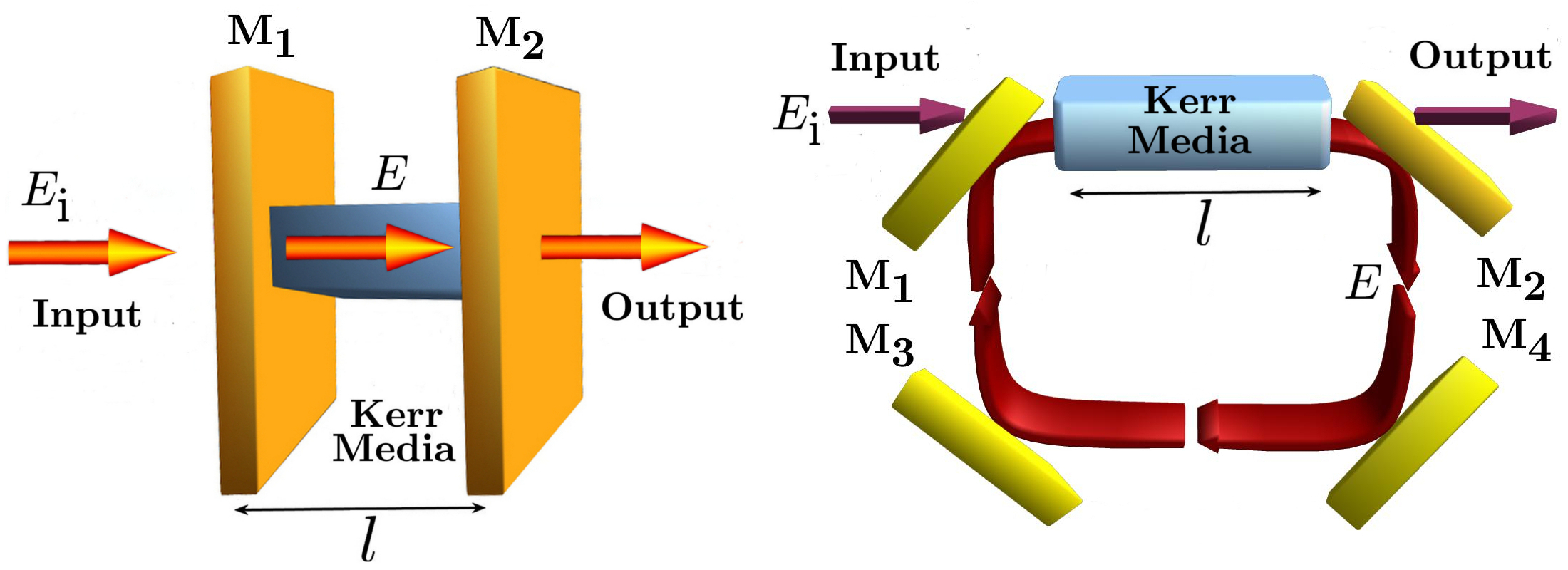
Figure 1: Schematic setups of optical cavities filled in with Kerr media. (a) Plane parallel cavity with length $l$ between the two mirrors $\textrm{M}_{1}$ and $\textrm{M}_{2}$. (b) Ring cavity between four mirrors. The input mirros $\textrm{M}_{1}$ and the output mirrors $\textrm{M}_{2}$ have high reflectivity and are partially transmitting, while $\textrm{M}_{3}$ and $\textrm{M}_{4}$ are fully reflecting.

When both 2D diffraction and 1D dispersion have a comparable influence during light propagation in a Kerr resonator, light bullet suffers collapse beam phenomena in the case of the 3D nonlinear Schrödinger equation Silberberg (1990); Edmundson (1997). By introducing additional physical effects, it is possible to avoid the collapse and to stabilise the LB formation. Several physical effect have been proposed in the literature such as Kerr cavities Tlidi et al. (1998a, b); Brambilla et al. (2004). The existence of stable LBs have been reported in other systems such as in wide-aperture lasers with a saturable absorber Kaliteevskiĭ and Rozanov (2000); Veretenov et al. (2000); Marconi et al. (2014); Javaloyes (2016); Dohmen et al. (2020), optical parametric oscillators Staliunas (1998); Veretenov and Tlidi (2009); Panoiu et al. (2005), second harmonic generation Tlidi and Mandel (1999); Tlidi (2000), passively mode-locked semiconductor lasers Grelu and Akhmediev (2012), left-handed materials Kockaert et al. (2006), twisted waveguide arrays Milián et al. (2019), in Swif-Hohenberg equation Staliunas (1998); Tlidi and Mandel (1999); Bordeu and Clerc (2015), and in the complex cubic-quintic Ginzburg–Landau equation Mihalache et al. (2006). (see recent reviews Malomed et al. (2005); Mihalache (2014); Malomed and Mihalache (2019)).

In broad area Kerr resonators light bullets are generated. They consist of self-organized structures that travel with the group velocity of the light within the cavity. Their stabilization is attributed to not only a balance between nonlinearity and diffraction/dispersion, but also the second balance that involves pumping or injection and dissipation or losses. This combined action of 1D dispersion and 2D diffraction in a Kerr resonator has revealed the existence of three-dimensional (3D) dissipative structures that can be spontaneously generated Tlidi et al. (1998a, b). Weakly nonlinear analysis and the relative stability analysis in the neighbourhood of 3D modulational instability has shown the predominance of the body-centered-cubic (bcc) lattice structure over other periodic structures such as lamellae, face-centered-cubic, or hexagonally packed cylinders. These analytical results however have never been checked numerically. The purpose of this paper is two fold: Firstly, to clarify the formation of optical crystals that emerge from the modulational instability, and secondly, to study the implication of the subcritical modulational instability on the formation of light bullets and clusters of them.

For this purpose, we consider optical resonators filled with a Kerr medium and coherently driven by an external injected field $E_{\textrm{i}}$. The schematic setup of a Fabry-Perot or a ring cavity setups are shown in Fig. 1. The transmitted part of this field interacts with the nonlinear media and suffers from nonlinearity, diffraction, chromatic dispersion, and losses. The physics of the Kerr optical resonator is best described by the paradigmatic Lugiato-Lefever equation (LLE) Lugiato and Lefever (1987). This model consists of a damped, and driven nonlinear Schrödinger equation, with detuning which was originally derived to describe diffractive spatial Kerr resonators. In this case, 2D diffraction ensures a coupling between different points in the transverse plane. When diffraction is neglected by using wave-guided structures such as fibers, the inclusion of the chromatic dispersion in the dispersive resonators leads also to the temporal LLE Haelterman et al. (1992). When 1D dispersion and 2D diffraction have a comparable influence, the formulation of this problem leads to the generalized Lugiato-Lefever equation Tlidi et al. (1998b, a)

$$\frac{\partial E}{\partial t}=E_{\textrm{i}}-(1+i\delta)E+\Big{(}\nabla_{\perp}^{2}+\frac{\partial^{2}}{\partial\tau^{2}}\Big{)}E+i|E|^{2}E,$$ (1)

where $E=E(x,y,t,\tau)\rightarrow(\kappa/\gamma l)^{1/2}E(x,y,t,\tau)$ is the normalized slowly-varying envelope of the electric field, with $\kappa$ being the total losses, $\gamma$ is the nonlinear coefficient, and $l$ is the cavity length. The detuning parameter $\delta=\phi/\kappa$ is the cavity detuning parameter where $\phi$ is the linear phase shift accumulated by the intracavity field over the cavity length $l$. The injected field $E_{\textrm{i}}\rightarrow\kappa(\kappa/\gamma\delta l)^{1/2}E_{\textrm{i}}$ is real, positive and constant assuming a continuous wave (CW) operation. The transverse Laplacian acting on the transverse plane $(x,y)$ is denoted by $\nabla_{\perp}^{2}$, and the second-order derivative term has a positive coefficient so that the cavity operates in the anomalous dispersion regime. In this case, the operator $\nabla_{\perp}^{2}+\partial^{2}_{\tau}=\partial^{2}_{x}+\partial^{2}_{y}+\partial^{2}_{\tau}$ is the 3D Laplacian acting in the Euclidian $(x,y,\tau)$ space. Time $t$ is the slow time describing the evolution over successive round trips, and $\tau$ is the fast time in the reference frame moving with the group velocity of the light within the cavity. In terms of physical parameters, the transverse coordinate, slow, and fast times are

$$(x,y)\rightarrow\sqrt{\frac{l}{2q\kappa}}(x,y),{\mbox{ }}(t,\tau)\rightarrow\Big{(}\frac{t_{r}}{\kappa}t,\sqrt{\frac{\beta_{2}l}{2\kappa}}\tau\Big{)},\\$$

where $t_{r}$ is the round trip time and $\beta_{2}$ denotes the second-order chromatic dispersion coefficient of the Kerr material. The LLE has been derived for other systems such as liquid crystals, left-handed materials Kockaert et al. (2006), and photonics coupled waveguides Peschel et al. (2004), whispering-gallery-mode microresonators Chembo and Menyuk (2013). In early reports, the LLE has been derived for a plasma driven by an external radiofrequency field Morales and Lee (1974) and for the condensate in the presence of an applied ac field Kaup and Newell (1978). Due to the richness of its broad spectrum of space-time dynamical behaviors, this simple model has attracted considerable theoretical and experimental investigations during these last decades, as witnessed by recent overviews Chembo et al. (2017); Lugiato et al. (2018).

The paper is organized as follows. In section 2II, we present numerical simulations of the LLE Eq. 1 showing indeed that the only stable optical crystals in the neighbourhood of the 2D modulational instability are indeed the bcc structures. This result has been established theoretically in previous reports in the weakly nonlinear regime Tlidi et al. (1998b, a) but never checked numerically. We construct the bifurcation diagram and we compare the results obtained by numerical simulation with these obtained through a normal form analysis. In section 3III, we consider a bistable regime where the 3D modulational instability appears subcritical. In this case, a pinning range of parameters exists where stable light-bullets and clusters of them can be generated. We construct their bifurcation diagram and we show that their domain of stability is wider than the monostable case studied recently. In addition, we obtain the stationary single light-bullet solution of the LLE Eq. 1 by using a spherical approximation, and we compare it with a direct numerical simulation of the governing equation in section 3III. We conclude in section 4IV.

II 3D modulational instablity and optical crystals

In 2D settings, numerical simulations indicate that only hexagonal structures are stable close to the modulational instability Firth et al. (1992); Tlidi et al. (1996). The weakly nonlinear analysis has allowed an investigation on the existence and stability of different periodic solutions, such as hexagons and stripes. The pattern selection analysis consists of studying the stability of one pattern to perturbations favoring another pattern Firth et al. (1992). This analysis is referred to as the relative stability analysis, and has shown analytically that stripes are not stable Tlidi et al. (1998b), which we confirm numerically in this study. The same analysis has been extended to 3D settings and has revealed the predominance of the body-centered-cubic (bcc) lattice structure over a variety of 3D structures in the cavity field intensity Tlidi et al. (1996). However, numerical simulations of 3D optical crystals are missing. The purpose of this paper is to bridge this gap and to present numerical simulations that confirm the analytical predictions obtained by the weakly nonlinear analysis.

Previous studies that have attempted to solve the 3D LLE (1) have used low-order finite-difference schemes coupled with low order Euler time stepping, which is indeed prone to numerical instabilities. This is mainly due to the fact that the LLE couples a stiff diffusion term with a strongly nonlinear term, which when discretised leads to large systems of strongly nonlinear stiff ordinary differential equations (ODEs) Jones and O’Brian (1996); Kassam (2004). In addition finite-difference methods can sometimes lead to spurious solutions which are non-physical Jones and O’Brian (1996), which is where higher-order spectral methods come to the fore. In the present work, the temporal discretisation is carried out with a fourth order exponential time differencing Runge–-Kutta method Trefethen (2000); Cox and Matthews (2002), and the spatial discretisation of the LLE is done using a Fourier spectral method with periodic boundary conditions Trefethen (2000); Kassam (2004); Saad (2011). In the resulting discretised set of ODEs the linear term is diagonal, which is one of the main advantages of using a Fourier spectral method. The nonlinear term is evaluated in physical space and then transformed to Fourier space. A detailed analysis on these methods can be found in these excellent books Trefethen (2000); Kassam (2004); Saad (2011) . In this study, we use a periodic domain of size $[0,80]^{3}$ units, which is found to be sufficient for the present study, discretised using $128$ grid points in each direction, with a time-step of $0.01$.

In the absence of diffraction and dispersion, the homogeneous steady state solutions of LLE, satisfying $\nabla_{\perp}^{2}E_{s}=0$, $\partial^{2}_{\tau}E_{s}=0$, and $\partial_{t}E_{s}=0$, are given by $E_{\textrm{i}}^{2}=|E_{s}|^{2}[1+(\delta-|E_{s}|^{2})^{2}]$. For $\delta<\sqrt{3}$, the transmitted intensity as a function of the input intensity $E_{\textrm{i}}^{2}$ is single-valued, whereas bistability occurs for $\delta>\sqrt{3}$. We consider small perturbations that depend on the coordinates $(x,y,t,\tau)$ in the form of plane waves $\exp{[i{\bf k_{\perp}}\cdot{\bf r}+ik_{\tau}\tau+\sigma t]}$. This formulation leads to the following characteristic equation

$$\sigma+2\sigma+\frac{\partial I_{s}}{\partial I_{i}}+(k^{2}_{\perp}+k^{2}_{\tau})[k^{2}_{\perp}+k^{2}_{\tau}-2(2I_{s}-\delta)]=0$$ (2)

where $\partial I_{s}/\partial I_{i}=1+(I_{s}-\delta)(I_{s}-2\delta)$ is the slope of the homogeneous steady states. These states undergo a modulational instability when $\sigma=0$, and $\partial\sigma/\partial k^{2}=0$ with $k^{2}=k^{2}_{\perp}+k^{2}_{\tau}$. The threshold associated with the MI is $E_{\textrm{ic}}^{2}=1+(\delta-1)^{2}$ for the injected field intensity. The corresponding intracavity intensity is $|E_{\textrm{c}}|^{2}=1$. At this bifurcation point, the wavelength of 3D patterns is $\Lambda=2\pi/\sqrt{2-\delta}$. When increasing the injected field above its value at the MI, there exists a finite band of Fourier modes $k$, $k^{2}_{\perp-}+k^{2}_{\tau-}<k^{2}_{\perp}+k^{2}_{\tau}<k^{2}_{\perp+}+k^{2}_{\tau+}$ with

$$k^{2}_{\perp\pm}+k^{2}_{\tau\pm}=2I_{s}-\delta\pm\sqrt{I_{s}^{2}-1},$$ (3)

which are linearly unstable and trigger the spontaneous evolution of the intracavity field towards a self-organized optical crystal. These structures consist of regular 3D lattices of bright spots traveling at the group velocity of light within the cavity.

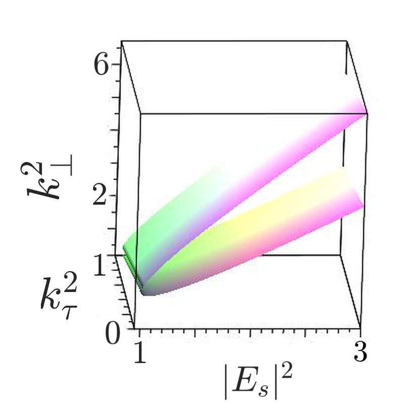
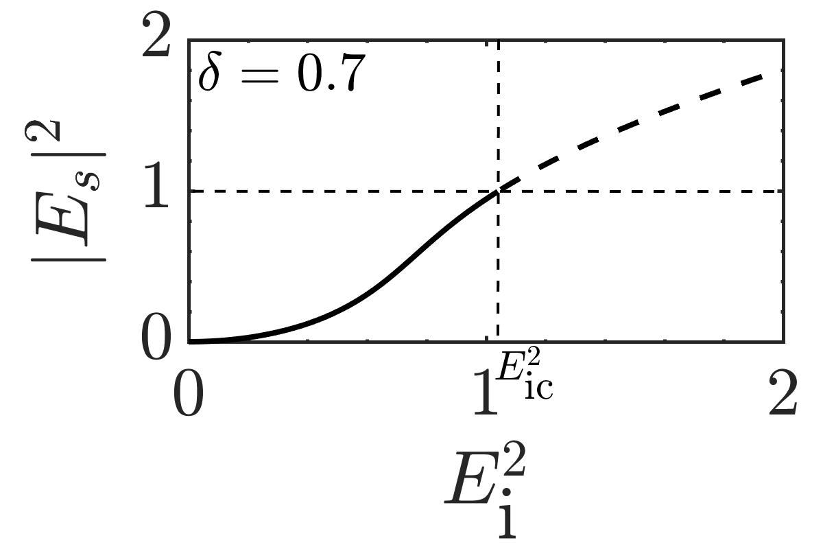
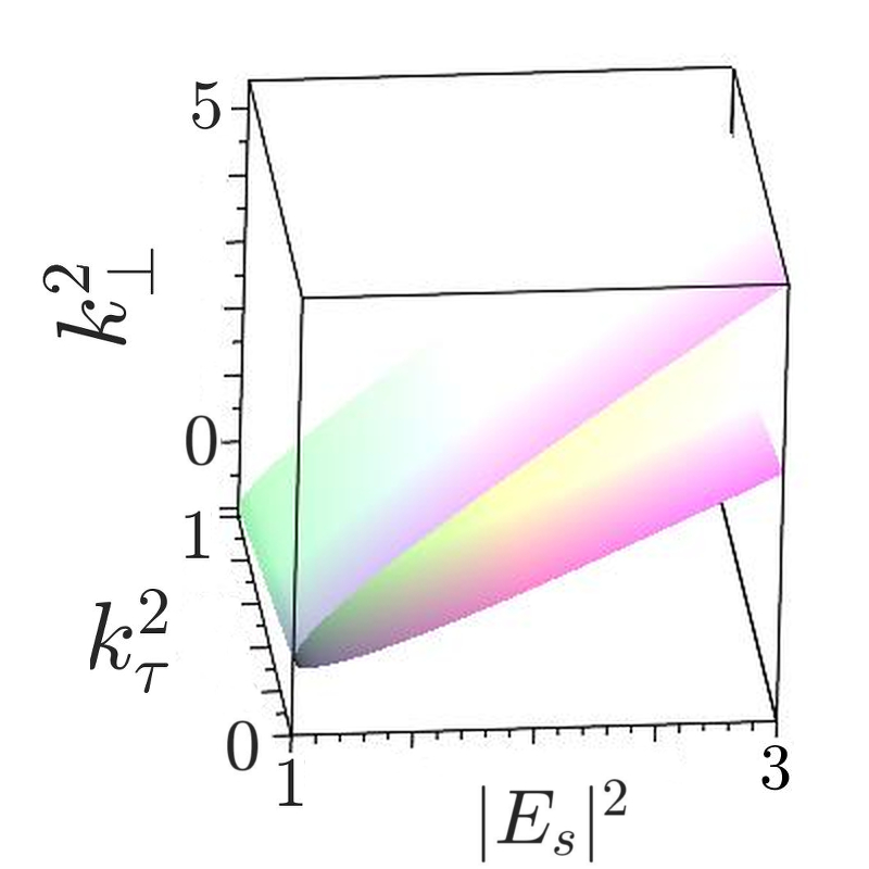
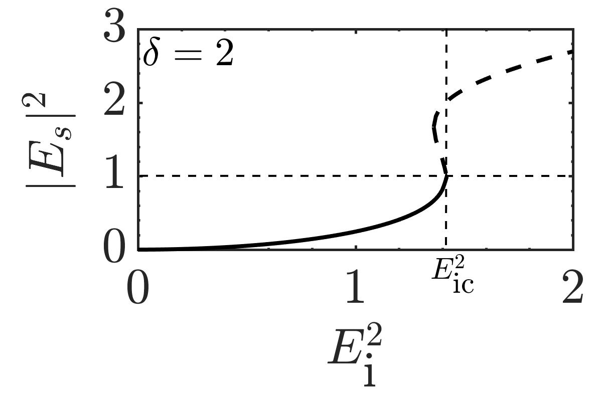
Figure 2: Homogeneous solution for $\delta=0.7$ and $\delta=2$. (a, c) Stable and unstable 3D modes in the plane $(|E_{s}|^{2},k^{2})$. The 3D wavenumbers corresponding to 2D diffraction and 1D dispersion given by $k^{2}=k^{2}_{\perp}+k^{2}_{\tau}$, with $k^{2}_{\perp}=k^{2}_{x}+k^{2}_{y}$. (b, d) Homogeneous steady states $|E_{s}|^{2}$ as a function of the input intensity $E^{2}_{\textrm{i}}$. This suffers a 3D modulational instability at $E_{\textrm{i}}=E_{\textrm{ic}}$. Broken lines correspond to unstable solutions.

The marginal stability curves together with the characteristic input-output are shown in Fig. 2 for two different values of the detuning parameter $\delta$. The number of unstable Fourier modes is much larger than in the 2D setting. These modes are arbitrarily directed in the Fourier space $(k_{x},k_{y},k_{\tau})$ since the system is isotropic in the Euclidean $(x,y,t,\tau)$ space. The maximum gain or the most unstable wave number is $k_{c}^{2}=k^{2}_{x}+k^{2}_{y}+k^{2}_{\tau}=2-\delta$. These modes form a sphere of radius $\sqrt{2-\delta}$ in Fourier space $(k_{x},k_{y},k_{\tau})$. There exists an indefinite number of modes generated with arbitrary directions. However, the nonlinear interaction allows for the generation and selection of regular crystals. Close to the MI threshold, three-dimensional periodic crystals, are approximated by a linear superposition of $n$ pairs of opposite wave vectors $k_{j}$ lying on the critical sphere of radius $\sqrt{2-\delta}$ as

$$E(\bf{r},t)=E_{s}+\bf{e}\sum_{j=1}^{n}A_{j}\exp{(\dot{\imath}\bf{r}\cdot\bf{k_{j}})}+c.c.$$ (4)

where c.c denotes the complex conjugate, and ${\bf{e}}=(2-\delta)/\delta$ is the eigenvector of the corresponding Jacobian matrix associated with the zero eigenvalue. The lamellae and rhombic structures are characterized by $n=1$ and $n=2$ respectively, and the 3D hexagons or hexagonally packed cylinders correspond to $n=3$ with $\sum_{j=1}^{3}\bf{k_{j}}=0$. The face-centered-cubic (fcc) lattice and the quasiperiodic crystals are obtained for $n=4$ and $n=5$, respectively. The body-centered-cubic (bcc) lattice corresponds to $n=6$ with the resonance conditions.

     

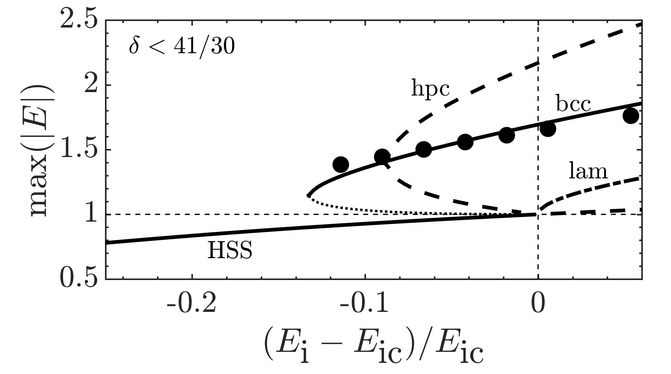
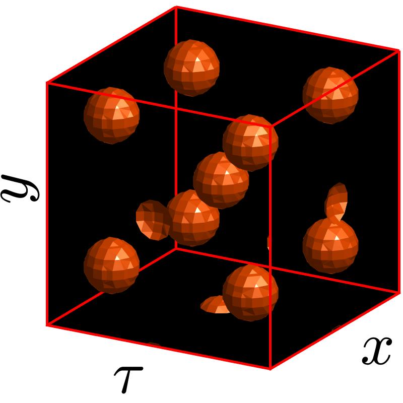
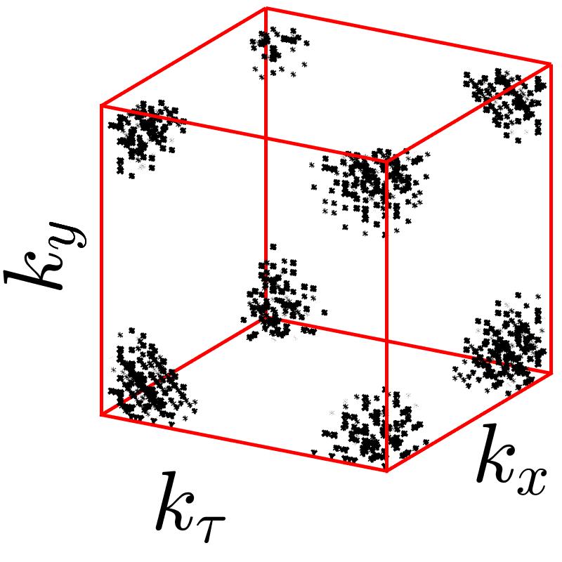
Figure 3: (a) Bifurcation diagram of the three-dimensional periodic patterns obtained from the weakly nonlinear analysis for $\delta=0.7$. Broken lines correspond to unstable solutions. The black dots along the bcc branch are the maximum values of the bcc solutions obtained by numerical simulations of the 3D LLE Eq. 1. (b) and (c) Isosurface of the intracavity field intensity corresponding to the 3D bcc solutions of Eq. 1 obtained from numerical simulations and its Fourier spectrum, respectively. Parameters are $E_{\textrm{i}}=1.05$ and $\delta=0.7$.

Applying a weakly nonlinear analysis that consists of seeking nonlinear solutions by using an expansion in terms of a small parameter which measures the distance from the Turing bifurcation, it has been shown in 2D settings that only triangular or hexagonal structures are stable, and transition from hexagons to stripes is not possible for the LLE Tlidi et al. (1998a). In 3D, an analytical calculation based on a weakly nonlinear analysis allows one to determine the variety and the stability properties of the three-dimensional dissipative crystals which are solutions of the generalized LLE Tlidi et al. (1998a, b). In these papers, the solvability condition allows for the derivation of amplitude equations for the critical modes associated with a set of finite modes. The most simple nonlinear solutions are lamellae, hexagonally packed cylinders (hpc), and body-centered-cubic (bcc) crystals. Their stationary solutions are $A_{lam}=(g/\alpha)^{1/2}$, $A_{hpc}^{\pm}=\left[-h_{2}\pm[h_{2}^{2}-4\alpha(2h_{1}-g)]^{1/2}]\right/2(2h_{1}-g)$,
$A_{bcc}^{\pm}=\left[-h_{2}\pm[h_{2}^{2}-\alpha(2h_{3}+5h_{1}-g)]^{1/2}]\right/(2h_{3}+5h_{1}-g)$, with $\alpha=(E_{\textrm{i}}-E_{ic})/E_{ic}(2-\theta)^{2}$, $g=[2(41-30\delta)]/9(1-(1-\delta)^{2})^{2},h_{1}=(4\delta-3)/[1-(1-\delta)^{2})2]$,$h_{2}=[1+F(E_{\textrm{i}}-E_{\textrm{ic}})]/[E_{\textrm{ic}}\theta]$, $F=[19(\delta^{3}-8)-4(23\delta^{3}-44\delta^{2}-14)]/2(2-\delta)^{4}[1+(2-\delta)^{2}]$, $h_{3}=-2[1+(1-\delta)^{2}]/[1-(1-\theta)^{2}]^{2}$. The relative linear stability analysis has been performed analytically and leads to the conclusion that only the most stable crystals are the bcc over others 3D nonlinear solutions Tlidi et al. (1998a). It has been remarked in the concluding remarks of this paper that these results are obtained in a perturbative way and therefore need further support from either numerical simulations or experimental evidence’ Tlidi et al. (1998a). We fill this gap by confirming the above pattern selection scenario by numerically integrating the LLE equation with periodic boundary conditions.

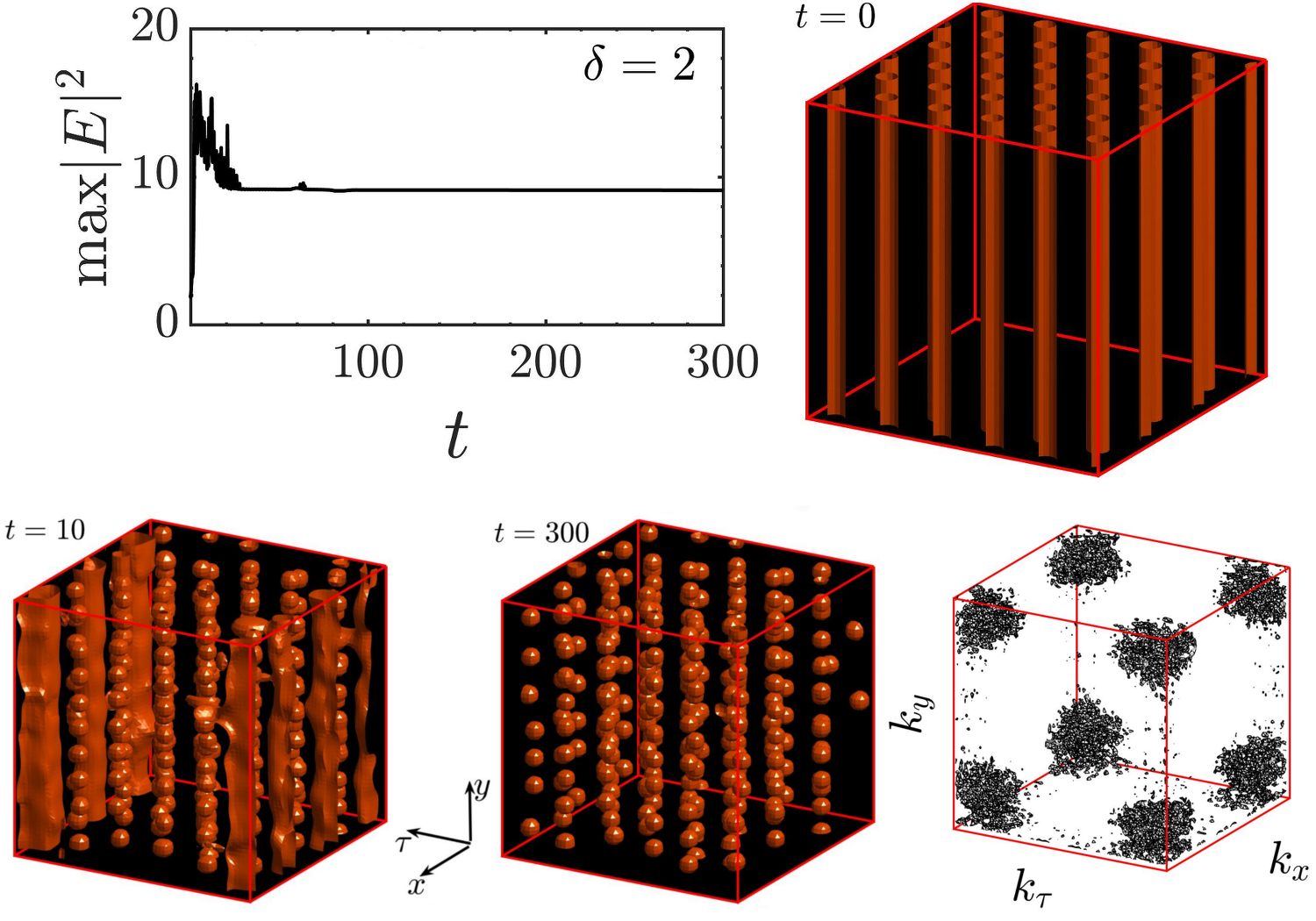
Figure 4: Destabilization of the hexagonally packed cylinder 3D structures towards the formation bcc crystals. Parameter settings: $E_{\textrm{i}}=1.42$ and $\delta=2.0$.

The results of the weakly nonlinear analysis are summarized in the bifurcation diagram displayed in Fig. 3(a). The stable bcc structure in Fig. 3(b) is obtained by time-marching the LLE using the coordinates of the associated stable wavevectors and their complex conjugates in wavenumber space, which are given by $k_{c}(\pm 1,\pm 1,0)/\sqrt{2},k_{c}(\pm 1,0,\pm 1)/\sqrt{2}$ and $k_{c}(0,\pm 1,\pm 1)/\sqrt{2}$, as the initial condition. The Fourier transform of the bcc structures is the fcc in Fourier space as shown in Fig. 3(c). We can see that lamella appears supercritically. This is because the above weakly nonlinear analysis has restricted the values of the detuning parameter to the range $\delta<\delta_{sub}$ with $\delta_{sub}<41/33$. The hpc and the bcc appear subcritically. However, lamellae and hpc are unstable, and only a branch of the bcc crystals emerges subcritically from the homogeneous solution at the bifurcation point. The bcc structures are unstable until a turning point given by $h_{2}^{2}=\alpha(2h_{3}+5h_{1}-g)$ is reached from which the branch $A_{bcc}$ emerges and is stable as shown in Fig. 3(a). To make explicit comparisons with analytical results, the numerical solutions are obtained for the parameter range where the system exhibits a monostable homogeneous steady-state solution and a supercritical modulational instability. The results of numerical simulations are shown by the black dots along the bcc branch of solutions (cf. Fig. 3(a)). From this comparison, we can see a good agreement. To show that the bcc crystals are the most stable solutions of the 3D LLE, we choose an initial condition consisting of a hexagonally packed cylinder as shown in Fig. 4. Time evolution of the system starting with this initial condition in which a small amplitude noise is added is shown in Fig. 4. In an earlier stage of time evolution, the cylinders break into spheres that interact and the system reaches a stable bcc crystal.

III Sub-critical modulational instability and localised light bullets

In the previous section, we have checked numerically that close to the 3D modulational instability the dynamics of the 3D Kerr cavity is predominated by the body-centered-cubic crystals over a variety of 3D structures in the cavity field intensity Tlidi et al. (1998b). The validity of this analysis is restricted to the values of the detuning parameter within the range $\delta<\delta_{sub}$ with $\delta_{sub}<41/33$. In what follows we focus on the strongly nonlinear regime where 3D modulational instability is subcritical, i.e., $\delta>\delta_{sub}$. Remarkably, besides the emergence of bcc structures, the same mechanism predicts the possible existence of stable of aperiodic distribution of dissipative light bullets. Recently, we have reported on the formation of LB in the monostable regime $\delta_{sub}<\delta<\sqrt{3}$ where the transmitted intensity, as a function of the input intensity is single-valued Gopalakrishnan et al. (2021). The results reported below describe the behavior predicted based on the 3D LLE Eq. 1, in a strongly nonlinear regime where the HSS exhibits a bistable regime $\delta>\sqrt{3}$. For this purpose, we fix the detuning parameter to $\delta=2$, and we let the injected field amplitude be the control parameter.

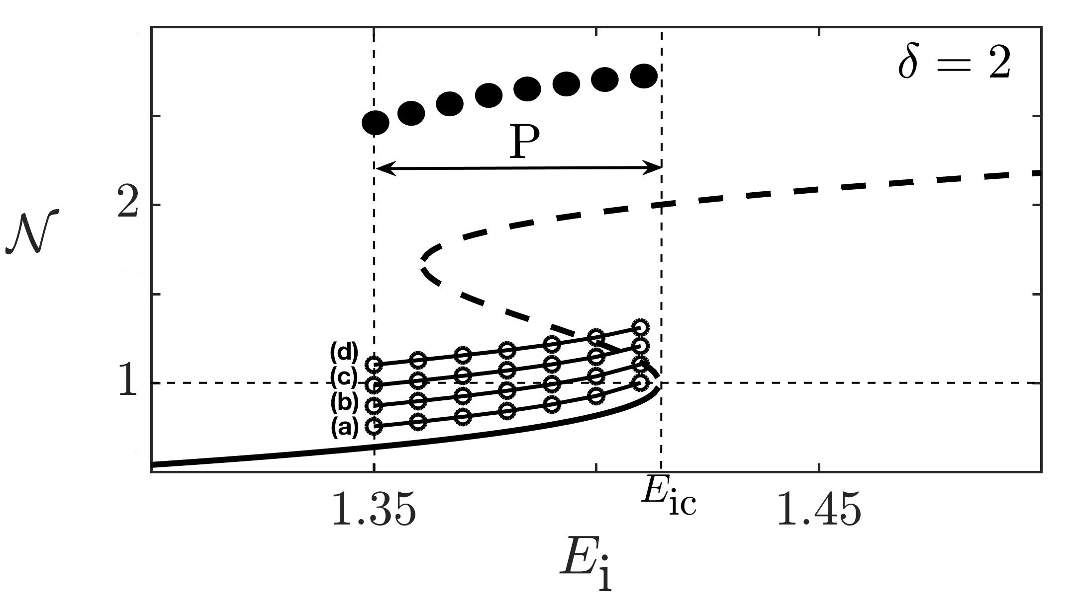
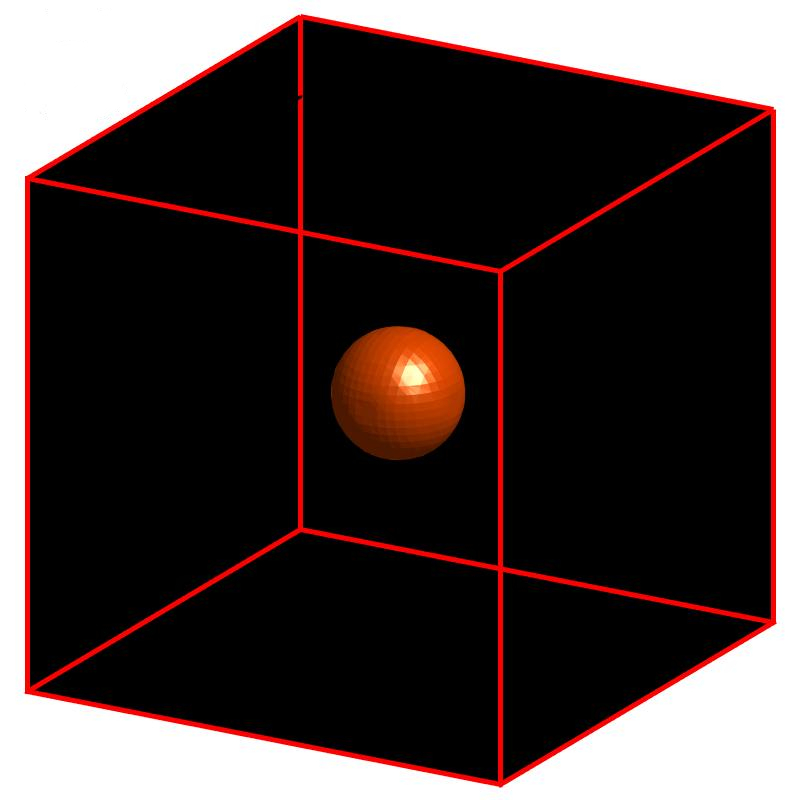
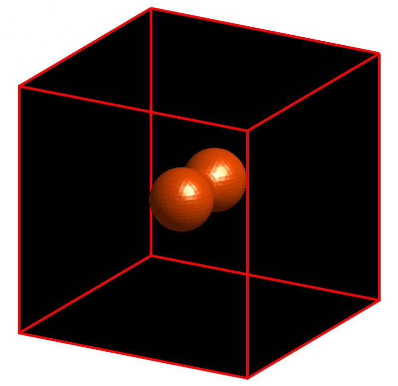
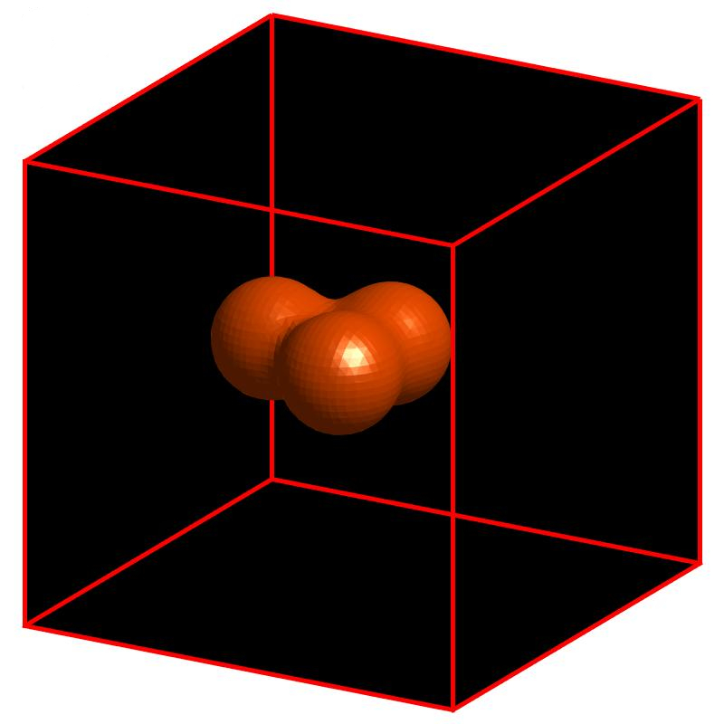
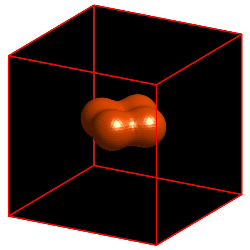
Figure 5: Bifurcation diagram associated with the LBs. The continuous black line denotes the stationary steady state. P indicates the pinning range. The black dots represent the corresponding values for the bcc solution. (a) A single elemental LB and (b,c,d) clusters of $2$, $3$, and $4$ LBs bounded together represented using the isosurfaces of the intracavity field intensity. Parameter settings: $E_{\textrm{i}}=1.40$ and $\delta=2$.

Figure 5 shows the homogeneous steady states together with the extended and periodic 3D dissipative structures. Numerical simulations showed that in the strongly nonlinear regime the bcc structures are the most stable crystals. The $L_{2}$ norm, defined below by Eq. 5, is plotted as a function of the injected field amplitude in Fig. 5. In this bifurcation diagram, the homogeneous steady states are plotted together with the bcc crystals. The upper branch of the bistable HSS curve is entirely unstable for the 3D modulation instability denoted by the dashed black line in Fig. 5. The $L_{2}$ norm associated with the bcc crystals is indicated by the black dot in Fig. 5. From this figure, we see a domain indicated by $P$ where the system exhibits multistability. The lower homogeneous steady states are represented by a continuous black line, and along with the bcc crystal, additional variety of aperiodic 3D structures can be obtained. Figure 5(a) shows a single stationary LB obtained numerically by using an initial condition consisting of a Gaussian shell centered in the computational domain. By placing multiple Gaussian shells and by varying the distances between them, one can obtain multiple robust stationary LBs within the optical cavity. Figure 5 shows two, three and four light bullets bounded together along different perspectives for $E_{\textrm{i}}=1.40$, and $\delta=2$. Indeed, once robust LBs have been obtained for a specific parameter setting, numerically they are used as the initial condition for further simulations, for instance, to obtain the bifurcation diagram for varying values of the amplitude of the injected field $E_{\textrm{i}}$. Since the amplitudes of LBs having different numbers of 3D peaks are more or less the same, it is convenient to plot the dimensionless “$L_{2}$ norm”,

$${\cal{N}}=\int|E-E_{s}|^{2}dx\,dy\,d\tau$$ (5)

as a function of the injected field amplitude $E_{\textrm{i}}$. Curves a,b,c,d in Fig. 5(a) shows the $L_{2}$ norm associated with LBs with $1$, $2$, $3$, and $4$ peaks. The single LB obtained by a direct numerical simulation of Eq. (1), can be solved under a spherical approximation. This approximation appears plausible since the LB is a stationary object with a spherical symmetry, and has the form $E(r)=E_{s}(1+A(r))$ with $r=(x^{2}+y^{2}+\tau^{2})^{1/2}$ and $E_{s}$ denotes the lower homogeneous steady state. By replacing this ansatz in the 3D LLE Eq. 1, and decomposing the intracavity field into real and imaginary parts as $E_{S}(r,z)=A_{r}+\dot{\imath}A_{i}(r)$, and by replacing the Laplace operator in polar coordinates $\nabla_{\perp}^{2}+\partial^{2}/\tau^{2}=\partial^{2}/\partial r^{2}+(2/r)\partial/\partial r$, we obtain four first order ODEs as

$$\frac{dy_{1}}{dr} = y_{2},$$

$$\frac{dy_{2}}{dr} = \delta y_{1}+y_{3}-\Big{(}y^{2}_{1}+y^{2}_{3}\Big{)}y_{1}-\frac{2y_{2}}{r},$$

$$\frac{dy_{3}}{dr} = y_{4},$$

$$\frac{dy_{4}}{dr} = E_{\textrm{i}}-y_{1}+\delta y_{3}-\Big{(}y^{2}_{1}+y^{2}_{3}\Big{)}y_{3}-\frac{2y_{4}}{r}.$$ (6)

where $y_{1}=A_{r},y_{2}=\frac{dA_{r}}{dr},y_{3}=A_{i},y_{4}=\frac{dA_{i}}{dr}$. We solve these set of equations as a boundary value problem for a finite value of $A_{r}$ at $r=0$, and $A_{r},A_{i}$ $\rightarrow 0$ as $r\rightarrow\infty$.

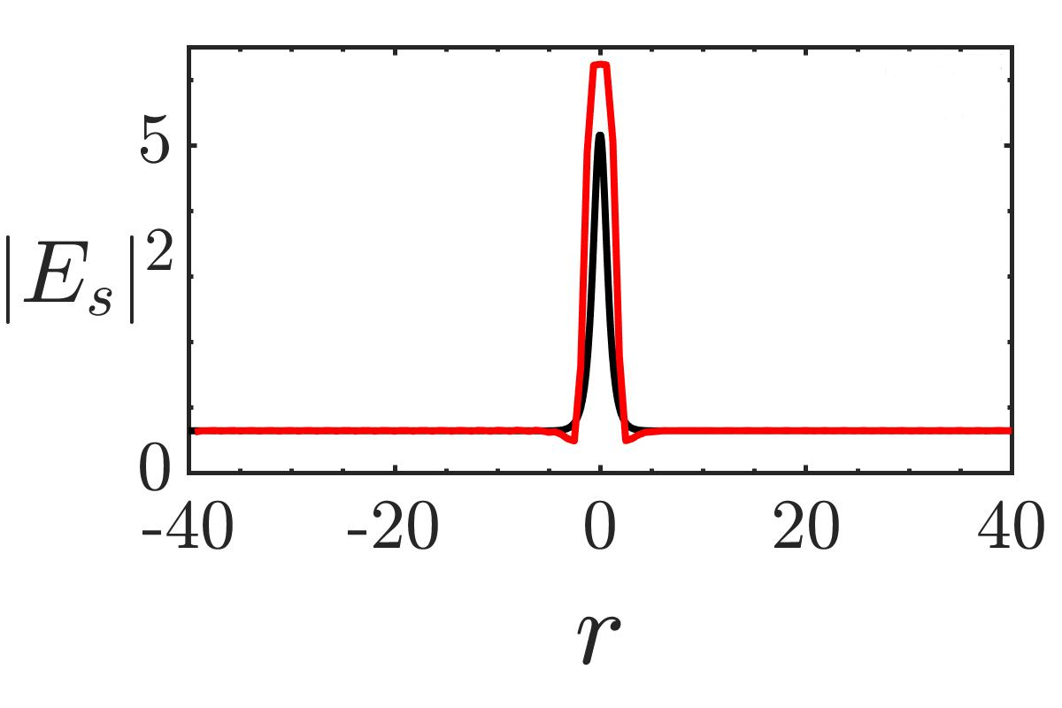
Figure 6: The real part of the steady-state solutions obtained using spherical symmetry considerations is shown in panels (a) and (c), with the total intensity shown using a black line in panels (b) and (d). The steady-state solution obtained by time-marching the LLE as discussed in the Letter is shown using a red line in panels (b) and (d) for comparison. Parameter settings are $\delta=2$ (a) $E_{\textrm{i}}=1.35$ (b) $E_{\textrm{i}}=1.40$.

Figure 6 shows the steady-state solution obtained by solving the above set of equations with the real part $A_{r}$ shown in panels (a, b), and $|E_{S}|^{2}$ in (b, d) in black respectively for $\delta=2.0$, and for two values of $E_{\textrm{i}}$. The solution obtained via integrating the LLE, is shown in red in panels (b, d) for comparison. The steady-state solutions obtained as a boundary value problem involves a careful choice in the initial amplitude for $A_{r}$ at $r=0$, and by imposing smooth conditions at $r=0$ as $dA_{r}/dr=dA_{i}/dr=0$. The present method has been used in earlier studies, for instance in Edmundson (1997) where the study focussed on the nonlinear Schrödinger equation. It can be noted in panels (b, d) that the oscillatory tail is more evident in the solutions obtained numerically by time-marching the LLE. although they are evident in both the solutions. Though the solutions are in good qualitative agreement, the absolute values of the intensity obtained using the two methods are slightly different. The steady-state solution obtained using spherical symmetry considerations by solving equations 6 as a boundary value problem has been carried out to qualitatively validate the results from the nonlinear simulations, rather than for precise quantitative comparisons.

Figure 7: Clusters of LBs coexisting along with an isolated LB. Parameter settings: $E_{\textrm{i}}=1.40$, $\delta=2$.

It should be noted that the LBs can bind themselves to each other via their oscillatory tails. We focus now on the situation where 3D peaks are close-packed so that their overlapping oscillatory tails interact strongly. All these LBs coexist as stable solutions with the bcc crystals in the range P shown in Fig. 5(a). The LBs are localized dissipative structures along the $x$, $y$, and $\tau$ directions. They can be seen as a cluster of the elemental structure (a single LB) with a well-defined size. Their position depends on the initial conditions, and the maximum of the coexisting LBs is essentially constant for fixed values of the system parameters.

As a final example of what 3D LLE Eq. 1 is able to generate, is clusters of LBs can coexist with a single isolated LB as shown in Fig. 7. Depending on the initial condition, we have also been able to find stable LBs with a few 3D peaks packed together forming a cluster of six LBs bounded together coexisting with a single LB. [see Fig. 7]. These two 3D localized objects are far away from each other. The distance between them is determined solely by the initial conditions used.

IV Discussion and concluding remarks

In conclusion, we have shown that the 3D lugiato-Lefever equation Eq. 1, captures quite a large variety of three-dimensional dissipative structures and clusters of light-bullets. In the first part, we have discussed the 3D pattern selection through the weakly nonlinear analysis and the relative stability analysis. We have checked numerically that the only possible periodic structures are the body-centered-cubic crystals. This n-analysis is restricted to the weakly nonlinear regime where close to the 3D modulational instability appears super-criticaly. The second part has been centered rather on the formation of light-bullet and clusters of them. We have shown that there exists a range of parameters called pinning zone where the system exhibits a multistability behavior. Besides the body-centered cubic crystals and the homogeneous steady states, another type of localized and aperiodic 3D structures have been generated for a fixed value of the system’s parameters.

The multiplicity of these 3D solutions of the LLE is strongly reminiscent of homoclinic snaking. The full diagram can be complex, and we displayed only four branches of LBs. Indeed, in one-dimensional settings, localized structures exhibit a homoclinic snaking bifurcation which has been established by continuation algorithms Gomila et al. (2007); Tlidi and Gelens (2010). The snaking bifurcation diagram consists of two snaking curves: one describes localized structures with $2n$ peaks, while the other corresponds to $2n+1$ peaks where $n$ is a positive integer. As one moves further along the snaking curve, the LB becomes better localized and acquires stability at the turning point where the slope becomes infinite. Outside of the pinning range, the LB begins to grow by adding extra peaks symmetrically at either side. This growth is associated with back and forth oscillations across the pinning range of the control parameter. This homoclinic snaking has been established first in Woods and Champneys (1999). An extension to two-dimensional settings of the homoclinic bifurcation has been discussed in recent overviews Lloyd et al. (2008); Knobloch (2015). However, continuation algorithms in 3D are still largely unexplored, and most of the results are obtained by direct numerical simulations of the governing equation.

Funding

K.P. acknowledges the support by the Fonds Wetenschappelijk Onderzoek-Vlaanderen FWO (G0E5819N) and the Methusalem Foundation. We also acknowledge the support from the French National Research Agency (LABEX CEMPI, Grant No. ANR-11- LABX-0007) as well as the French Ministry of Higher Education and Research, Hauts de France council and European Regional Development Fund (ERDF) through the Contrat de Projets Etat-Region (CPER Photonics for Society P4S). M.T acknowledges financial support from the Fonds de la Recherche Scientifique FNRS under Grant CDR no. 35333527 ”Semiconductor optical comb generator”. A part of this work was supported by the ”Laboratoire Associé International” University of Lille - ULB on ”Self-organisation of light and extreme events” (LAI-ALLURE).”

References

- Cross and Hohenberg (1993) Mark C Cross and Pierre C Hohenberg, “Pattern formation outside of equilibrium,” Reviews of modern physics 65, 851 (1993).
- Arecchi et al. (1999) F Tito Arecchi, Stefano Boccaletti, and PierLuigi Ramazza, “Pattern formation and competition in nonlinear optics,” Physics Reports 318, 1–83 (1999).
- Staliunas and Sánchez-Morcillo (2003) K. Staliunas and V. Sánchez-Morcillo, Transverse patterns in nonlinear optical resonators. Springer Tracts in Modern Physics (Berlin, Germany: Springer., 2003).
- Murray (2007) James D Murray, Mathematical biology: I. An introduction, Vol. 17 (Springer Science & Business Media, 2007).
- Akhmediev and (eds) N. Akhmediev and A. Ankiewicz (eds)., Dissipative solitons: from optics to biology and medicine. (Lecture Notes in Physics, vol. 751. Heidelberg, Germany: Springer., 2008).
- Tlidi et al. (2014) M. Tlidi, K. Staliunas, K. Panajotov, A. G. Vladimirov, and M. G. Clerc, “Localized structures in dissipative media: from optics to plant ecology,” Phil. trans. R. Soc. A 372, 20140101 (2014).
- Tlidi and Clerc (2016) Mustapha Tlidi and Marcel G Clerc, “Nonlinear dynamics: Materials, theory and experiments,” Springer Proceedings in Physics 173 (2016).
- Lugiato et al. (2018) LA Lugiato, F Prati, ML Gorodetsky, and TJ Kippenberg, “From the Lugiato–Lefever equation to microresonator-based soliton kerr frequency combs,” Philosophical Transactions of the Royal Society A: Mathematical, Physical and Engineering Sciences 376, 20180113 (2018).
- Tlidi et al. (2018) Mustapha Tlidi, MG Clerc, and Krassimir Panajotov, “Dissipative structures in matter out of equilibrium: from chemistry, photonics and biology, the legacy of ilya prigogine (part 1),” (2018).
- Fortier and Baumann (2019) Tara Fortier and Esther Baumann, “20 years of developments in optical frequency comb technology and applications,” Communications Physics 2, 1–16 (2019).
- Scorggie et al. (1994) A. J. Scorggie, W. J. Firth, G. S. McDonald, M. Tlidi, R. Lefever, and L. A. Lugiato, “Pattern formation in a passive Kerr cavity,” Chaos Solitons Fract. 4, 1323 (1994).
- Taranenko et al. (2000) V. B. Taranenko, I. Ganne, R. J. Kuszelewicz, and C. O. Weiss, “Patterns and localized structures in bistable semiconductor resonators,” Phys. Rev. A 61, 063818 (2000).
- Taranenko et al. (2001) VB Taranenko, I Ganne, R Kuszelewicz, and CO Weiss, “Spatial solitons in a semiconductor microresonator,” Applied Physics B 72, 377–380 (2001).
- Barland et al. (2002) S. Barland, J. R. Tredicce, M. Brambilla, L. A. Lugiato, S. Balle, M. Giudici, T. Maggipinto, L. Spinelli, G. Tissoni, T. Knoedl, M. Miller, and R. Jaeger, “Cavity solitons as pixels in semiconductor microcavities,” Nature 419, 699–702 (2002).
- Silberberg (1990) Y. Silberberg, “Collapse of optical pulses,” Opt. Lett. 15, 1282 (1990).
- Edmundson (1997) D. E. Edmundson, “Unstable higher modes of three-dimensional nonlinear Schrödinger equation,” Phys. Rev. E 55, 7636 (1997).
- Tlidi et al. (1998a) M. Tlidi, M. Haelterman, and P. Mandel, “3D patterns and pattern selection in optical bistability,” Europhys. Lett. 42, 505–509 (1998a).
- Tlidi et al. (1998b) M. Tlidi, M. Haelterman, and P. Mandel, “Three-dimensional structures in diffractive and dispersive nonlinear ring cavities,” Quantum Semiclass. Opt. 10, 869–878 (1998b).
- Brambilla et al. (2004) M. Brambilla, T. Maggipinto, G. Patera, and L. Columbo, “Cavity light bullets: Three-dimensional localized structures in a nonlinear optical resonator,” Phys. Rev. Lett. 93, 203901 (2004).
- Kaliteevskiĭ and Rozanov (2000) N. A. Kaliteevskiĭ and N. N. Rozanov, “On three-dimensional dissipative optical solitons: Collisions of laser bullets and topological solitons,” Opt. Spect. 89, 569–573 (2000).
- Veretenov et al. (2000) N. A. Veretenov, A. G. Vladimirov, N. A. Kaliteevskiǐ, N. N. Rozanov, S. V. Fedorov, and A. N. Shatsev, “Conditions for the existence of laser bullets,” Opt. Spectrosc. 89, 380 (2000).
- Marconi et al. (2014) M. Marconi, J. Javaloyes, S. Balle, and M. Giudici, “How lasing localized structures evolve out of passive mode locking,” Phys. Rev. Lett. 112, 223901 (2014).
- Javaloyes (2016) J. Javaloyes, “Cavity light bullets in passively mode-locked semiconductor lasers,” Phys. Rev. Lett. 116, 043901 (2016).
- Dohmen et al. (2020) F. Dohmen, J. Javaloyes, and S. V. Gurevich, “Bound states of light bullets in passively mode-locked semiconductor lasers,” Chaos 30, 063120 (2020).
- Staliunas (1998) K. Staliunas, “Three-dimensional Turing structures and spatial solitons in optical parametric oscillators,” Phys. Rev. Lett. 81, 81–84 (1998).
- Veretenov and Tlidi (2009) N. A. Veretenov and M. Tlidi, “Dissipative light bullets in an optical parametric oscillator,” Phys. Rev. A 80, 023822 (2009).
- Panoiu et al. (2005) N. -C. Panoiu, R. M. Osgood, Jr., B. A. Malomed, F. Lederer, D. Mazilu, and D. Mihalache, “Parametric light bullets supported by quasi-phase-matched quadratically nonlinear crystals,” Phys. Rev. E 71, 036615 (2005).
- Tlidi and Mandel (1999) M. Tlidi and P. Mandel, “Three-dimensional optical crystals and localized structures in cavity second harmonic generation,” Phys. Rev. Lett. 83, 4995 (1999).
- Tlidi (2000) Mustapha Tlidi, “Three-dimensional crystals and localized structures in diffractive and dispersive nonlinear ring cavities,” Journal of Optics B: Quantum and Semiclassical Optics 2, 438 (2000).
- Grelu and Akhmediev (2012) P. Grelu and N. Akhmediev, “Dissipative solitons for mode-locked lasers.” Nat. Photonics 6, 84 (2012).
- Kockaert et al. (2006) Pascal Kockaert, Philippe Tassin, Guy Van der Sande, Irina Veretennicoff, and Mustapha Tlidi, “Negative diffraction pattern dynamics in nonlinear cavities with left-handed materials,” Physical Review A 74, 033822 (2006).
- Milián et al. (2019) C. Milián, Y. V. Kartashov, and L. Torner, “Robust ultrashort light bullets in strongly twisted waveguide arrays,” Phys. Rev. Lett. 123, 133902 (2019).
- Bordeu and Clerc (2015) Ignacio Bordeu and Marcel G. Clerc, “Rodlike localized structure in isotropic pattern-forming systems,” Phys. Rev. E 92, 042915 (2015).
- Mihalache et al. (2006) Dumitru Mihalache, D Mazilu, F Lederer, Yaroslav V Kartashov, L-C Crasovan, L Torner, and BA Malomed, “Stable vortex tori in the three-dimensional cubic-quintic ginzburg-landau equation,” Physical Review Letters 97, 073904 (2006).
- Malomed et al. (2005) B. A. Malomed, D. Mihalache, F. Wise, and L. Torner, “Spatiotemporal optical solitons,” J. Opt. B: Quantum Semiclass. Opt. 7, R53–R72 (2005).
- Mihalache (2014) D. Mihalache, “Multidimensional localized stuctures in optics and Bose–Einstein condensates: a selection of recent studies.” Rom. J. Phys. 59, 295 (2014).
- Malomed and Mihalache (2019) B. A. Malomed and D. Mihalache, “Nonlinear waves in optical and matter-wave media: a topical survey of recent theoretical and experimental results.” Rom. J. Phys. 64, 106 (2019).
- Lugiato and Lefever (1987) L. A. Lugiato and R. Lefever, “Spatial dissipative structures in passive optical systems,” Phys. Rev. Lett. 58, 2209 (1987).
- Haelterman et al. (1992) Marc Haelterman, Stefano Trillo, and Stefan Wabnitz, “Dissipative modulation instability in a nonlinear dispersive ring cavity,” Optics communications 91, 401–407 (1992).
- Peschel et al. (2004) U Peschel, O Egorov, and F Lederer, “Discrete cavity solitons,” in Nonlinear Guided Waves and Their Applications (Optical Society of America, 2004) p. WB6.
- Chembo and Menyuk (2013) Y. K. Chembo and C. R. Menyuk, “Spatiotemporal Lugiato–Lefever formalism for Kerr-comb generation in whispering-gallery-mode resonators,” Phys. Rev. A 87, 053852 (2013).
- Morales and Lee (1974) GJ Morales and YC Lee, “Ponderomotive-force effects in a nonuniform plasma,” Physical Review Letters 33, 1016 (1974).
- Kaup and Newell (1978) David James Kaup and Alan C Newell, “Theory of nonlinear oscillating dipolar excitations in one-dimensional condensates,” Physical Review B 18, 5162 (1978).
- Chembo et al. (2017) Yanne K Chembo, Damià Gomila, Mustapha Tlidi, and Curtis R Menyuk, “Theory and applications of the Lugiato–Lefever equation,” (2017).
- Firth et al. (1992) W. J. Firth, A. J. Scroggie, G. S. McDonald, and L. A. Lugiato, “Hexagonal patterns in optical bistability,” Phys. Rev. A 46, R3609–R3612 (1992).
- Tlidi et al. (1996) M. Tlidi, R. Lefever, and P. Mandel, “Pattern selection in optical bistability,” Quantum Semicalss. Opt. 8, 931–938 (1996).
- Jones and O’Brian (1996) W. B. Jones and J. O’Brian, “Pseudo-spectral methods and linear instabilities in reaction-diffusion fronts,” Chaos 6, 219–228 (1996).
- Kassam (2004) A.-K. Kassam, High order timestepping for stiff semilinear partial differential equations (University of Oxford, 2004).
- Trefethen (2000) L. N. Trefethen, Spectral Methods in MATLAB (SIAM, Philadelphia, 2000).
- Cox and Matthews (2002) S. M. Cox and P. C. Matthews, “Exponential time differencing for stiff systems,” J. Comput. Phys. 176, 430–455 (2002).
- Saad (2011) Y. Saad, Numerical methods for large eigenvalue problems (SIAM, 2011).
- Gopalakrishnan et al. (2021) Shyam Sunder Gopalakrishnan, Krassimir Panajotov, Majid Taki, and Mustapha Tlidi, “Dissipative light bullets in kerr cavities: Multistability, clustering, and rogue waves,” Physical review letters 126, 153902 (2021).
- Gomila et al. (2007) Damia Gomila, Andrew J Scroggie, and William J Firth, “Bifurcation structure of dissipative solitons,” Physica D: Nonlinear Phenomena 227, 70–77 (2007).
- Tlidi and Gelens (2010) Mustapha Tlidi and Lendert Gelens, “High-order dispersion stabilizes dark dissipative solitons in all-fiber cavities,” Optics letters 35, 306–308 (2010).
- Woods and Champneys (1999) P. D Woods and A. R Champneys, “Heteroclinic tangles and homoclinic snaking in the unfolding of a degenerate reversible Hamiltonian–Hopf bifurcation,” Physica D: Nonlinear Phenomena 129, 147–170 (1999).
- Lloyd et al. (2008) David JB Lloyd, Björn Sandstede, Daniele Avitabile, and Alan R Champneys, “Localized hexagon patterns of the planar swift–hohenberg equation,” SIAM Journal on Applied Dynamical Systems 7, 1049–1100 (2008).
- Knobloch (2015) E Knobloch, “Spatial localization in dissipative systems,” conmatphys 6, 325–359 (2015).