Horizontal muon track identification with neural networks in HAWC

Abstract

Nowadays the implementation of artificial neural networks in high-energy physics has obtained excellent results on improving signal detection. In this work we propose to use neural networks (NNs) for event discrimination in HAWC. This observatory is a water Cherenkov gamma-ray detector that in recent years has implemented algorithms to identify horizontal muon tracks. However, these algorithms are not very efficient. In this work we describe the implementation of three NNs: two based on image classification and one based on object detection. Using these algorithms we obtain an increase in the number of identified tracks. The results of this study could be used in the future to improve the performance of the Earth-skimming technique for the indirect measurement of neutrinos with HAWC.

1 Earth-skimming neutrino detection with HAWC

The HAWC observatory consists of a large 22,000 $m^{2}$ area densely covered with 300 water Cherenkov detectors (WCDs) [1]. This laboratory is an instrument sensitive to hadron and gamma ray air showers in the TeV energy regime, and it has been in operation since 2015. HAWC has a 2$sr$ instantaneous field of view between declinations $\delta$ $\in$ [-26°,+64°], covering $2/3$ of the sky every 24 hours [2]. Nowadays there is an alternative line of research that proposes to use this observatory as an indirect neutrino detector [3, 4]. This idea is based on the Earth-skimming technique, here we want to get an interaction between a neutrino and a nucleon in a high mass target by exchanging a $W^{\pm}$ boson, the result of this interaction produces a charged lepton with the same flavor of the incoming neutrino. HAWC is located at an altitude of 4100 m a.s.l. in the vicinity of the mountain Pico de Orizaba in Mexico, this mountain is used as target to produce the neutrino-nucleon reaction. The tau leptons produced by a neutrino in this type of interaction are the most likely to be detected in any of the HAWC detectors. It should be noted that the muons generated in an air shower in the same direction of the Pico de Orizaba represent the main source of noise for this neutrino signals. One of the characteristics of these noise signals and neutrino signals is that they must activate a line of detectors from the HAWC observatory; furthermore, their trajectory must be quasi horizontal because they passed through of the Mountain. For this reason, we are going to refer to this type of signals as "horizontal tracks". In [4] is described one of the method to detect horizontal tracks in HAWC. The phases of this method is:

1. Triggering of candidate signals using the HAWC shower data.

2. Tracking algorithm.

3. Filtering of candidate tracks.

In the first two steps, most of the air shower events are eliminated; but the sample is still contaminated with very inclined small showers. For this reason, a series of filters are applied in the last step. In this work we propose to train a convolutional neural network (CNN) to replace these filters, with this change we analyze the possibility of increasing the number of identified tracks.

1.1 CNN: Image classification

Image classification is one of the most common applications for a CNN. In high energy physics there is a great variety of uses for this application. For example, the NEXT [5] experiment used a CNN for the identification of electron-positron pair production events, which exhibit a topology similar to that of a neutrinoless double-beta decay event. Also in [6] present CNN for signal/background discrimination for classification based on simulated data from the Ice Cube neutrino observatory and an ATLAS-like detector. So in this work we use a CNN to classify horizontal tracks events and air shower events. Figure 1 shows a visual comparison between these two events. The small circles represent the photomultipliers (PMTs) in each tank. The color in the PMTs represent the activation time in the event and the size symbolize the charge detected. The events are more easy to recognize using an image (figure 1) because their shape is different. Thus, we analyze the possibility of applying a CNN for track discrimination.

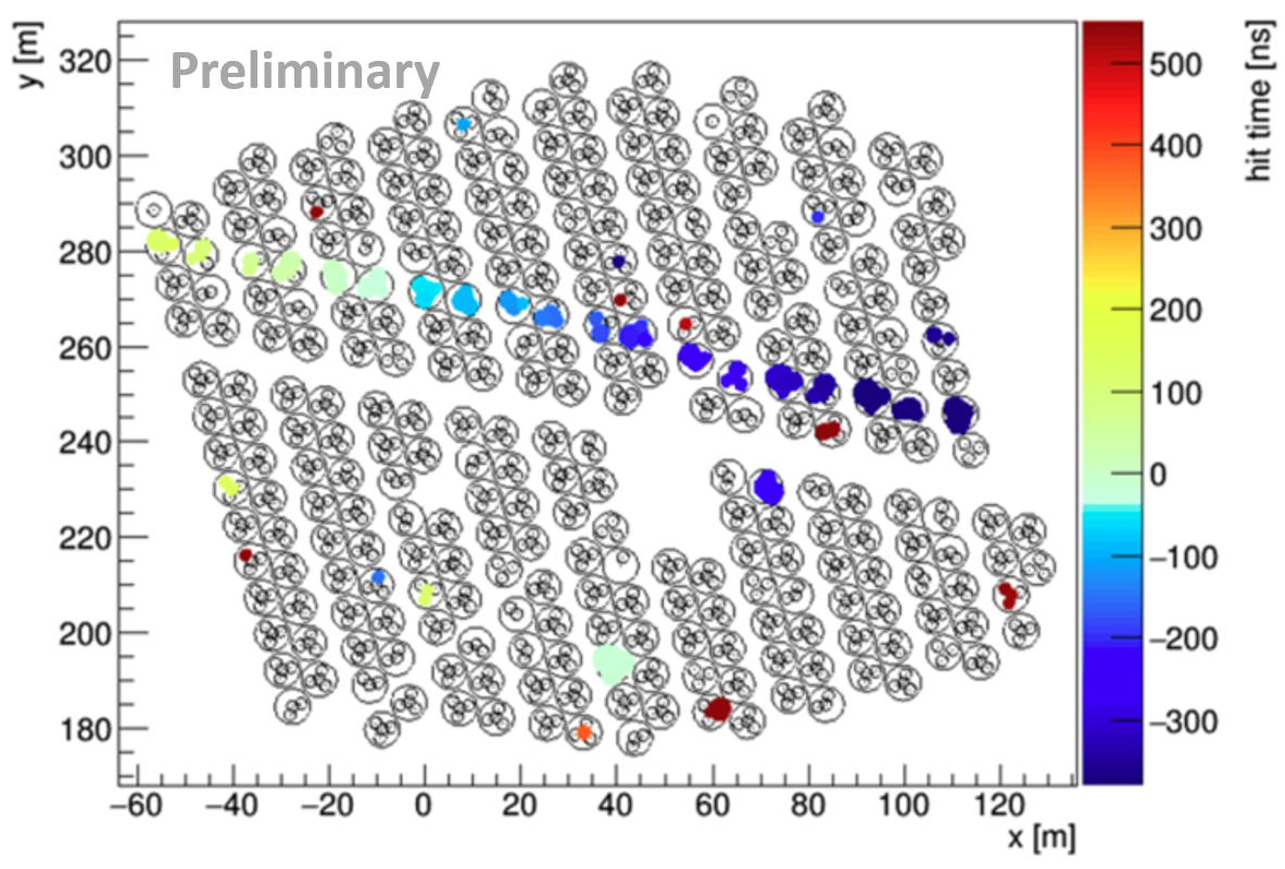
(a) Horizontal track.

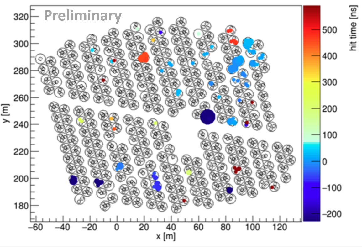
(b) Air Shower.

Figure 1: Visual comparison between a horizontal track and an air shower.

1.1.1 Network architecture

We use the convolutional network model VGG16, which is a pre-trained network with 13 convolutional layers and 3 fully connected layers. VGG16 is a convolutional neural network model proposed by K. Simonyan and A. Zisserman in the paper [7]. The model achieves 92.7 % top-5 test accuracy in ImageNet, which is a dataset of over 14 million images belonging to 1000 classes. For this work, the network output is a real number between zero and one. If the value is closer to zero, then it is more likely to be a track.

1.1.2 Dataset

The selection of the data used in training and testing stage is described following:

1. We use the candidates given by the Tracking algorithm described in [4].

2. We apply a selection cut to the possible tracks given by the previous step. With this cut, we take the candidates with beta values ($\beta=v\textfractionsolidus c$) between 0.5 and 1.5. We choose this range because we are looking for signals with a speeds close to the light that spread in a straight line. To calculate the speed, we use the average length and the central PMT time between the first and the last tank that was activated in the event.

3. Finally, we generate the images of the events that we obtained in the previous step.

We tested 2 different models of CNN focused on image classification. Both models used the same network architecture, but different training images. We named model A to the network in which we use the normal image given by the official HAWC display (an example is shown in figure 1 a). On the other hand for model B we remove from the image the PMTs that were not activated, an example for this event is shown in the figure 2. As this model used a clearer imagen, we analyze the improvement of this model with respect to model A.

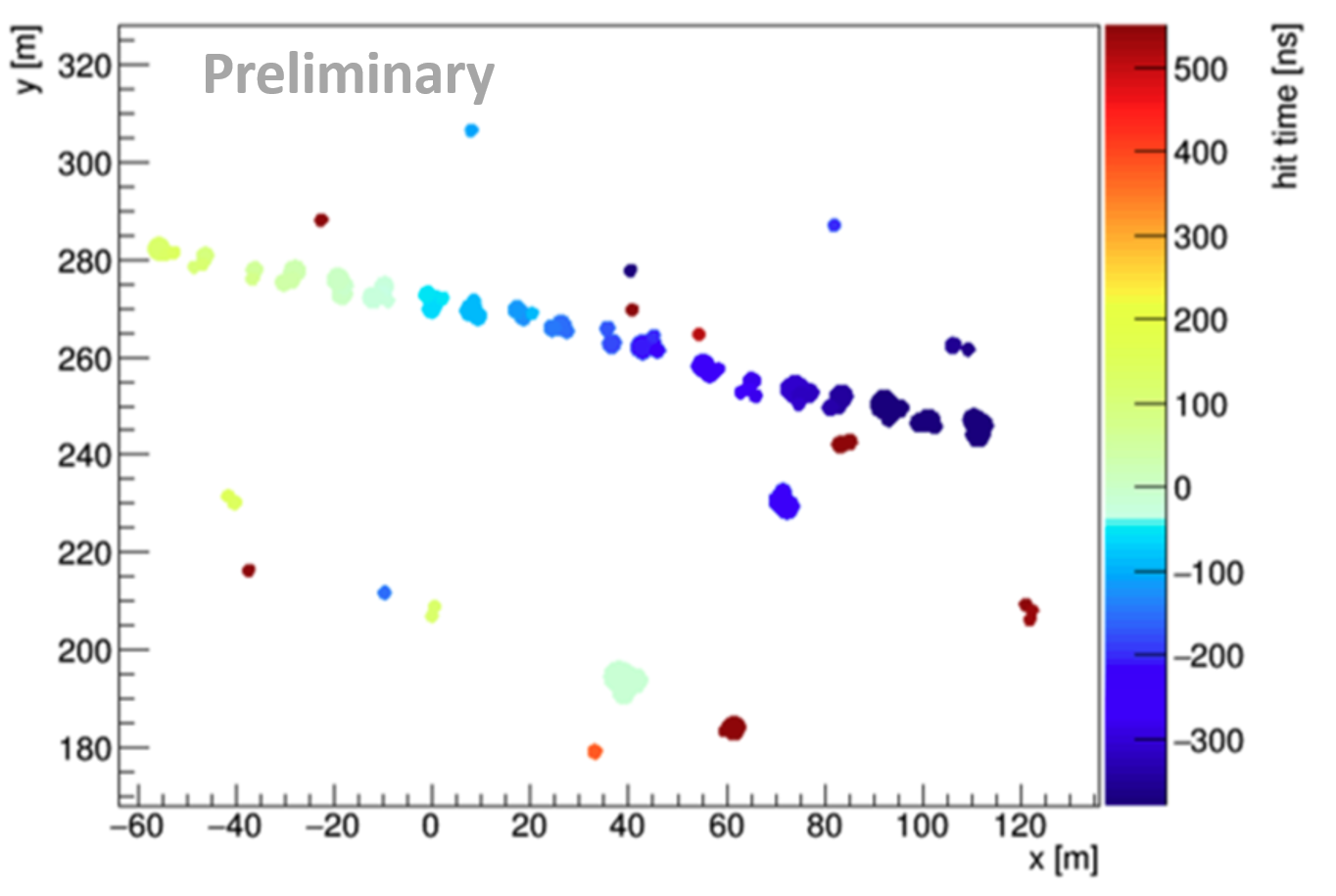
Figure 2: Event display without tanks. This type of image was use in model B.

Finally, we hand-sort images of tracks and air showers that passed the $\beta$ filter to make the following training and test sets.

• Training dataset: We used 1050 tracks images and 5627 air shower images. Then, with this dataset we made the training for the network. After that, we passed 8426 air shower images to the trained model and all the false positives were added to the training data.

• Validation dataset: We used 116 tracks images and 116 air shower images. This set is used to calculate the loss function and the success rate in each of the training steps.

• Test dataset: We used 100 tracks images and 1000 air shower images that passed the $\beta$ filter. The proportion of this set is like the number of tracks and air showers in the real data and we use it to see the behavior of our networks when we will analyze real events.

Model A and B used the same number of horizontal tracks and air showers described in the training and test data.

1.1.3 Results

To evaluate the model, we use the loss function and success rate. Loss function quantifies the error between predicted and output values, and the success rate tells us the proportion of correctly classified events. For both models, we calculate these variables in 50 training steps or epochs, the results are shown in figure 3. In these plots, the blue line is for training data and the yellow line is for test data; also the dotted line is for model A and the solid line is for model B. The loss for the training data is decreasing in each training step, however for test data the loss begins to increase from the 22th epoch. This is a clear sign that the network is specializing in training data (we have overfitting). For this reason, we use the both trained model until the step 20. On the other hand, the success rate for the test images was around 70% for both models. We have a relatively low percentage of this variable because the network just identifies correctly one fifth of the horizontal tracks images. However, both models correctly classify almost all the air showers images.

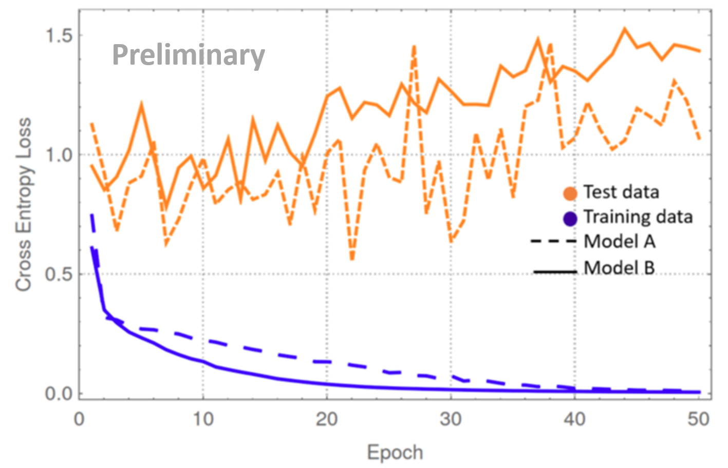
(a) Loss function.

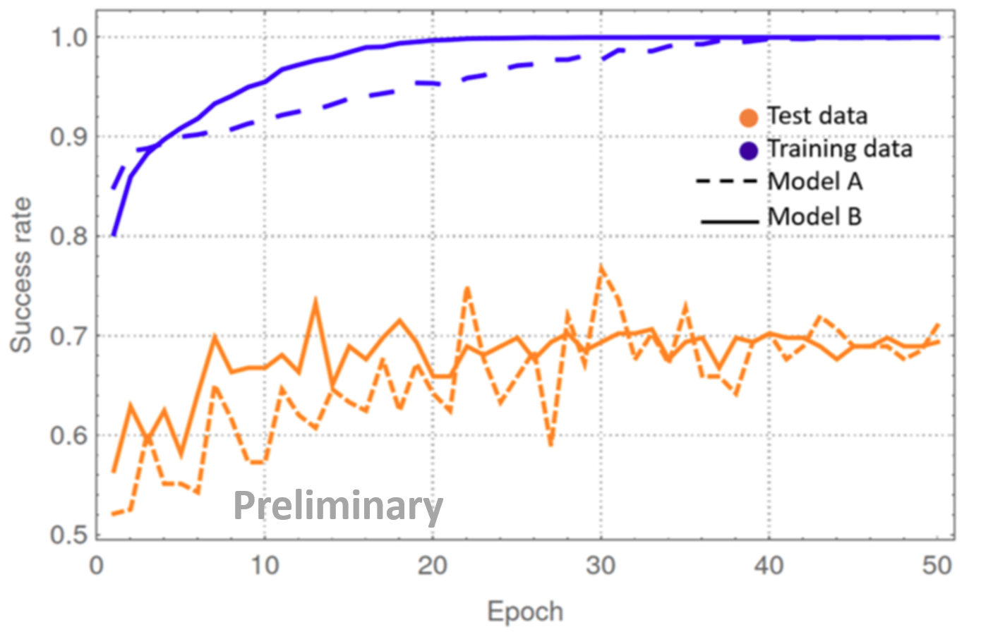
(b) Success rate

Figure 3: Loss and success rate for both models A and B.

For this work an event classified as a track was taken as positive and an event classified as an air shower was negative, so taking this into account, we also use the following variables to test the models:

• Precision Proportion of positive identifications that was correct. In our case, it indicates the proportion of tracks classified correctly.

• Recall: Proportion of all positive identifications that was correct.

In figure 4 we show a precision vs recall plot for model A and model B to analyze the percentage of tracks identified by the network that were correct. This plot was made for different threshold values and using the second test dataset. Remember that the output of the network is a real number between zero and one. So, threshold value is the number from which we consider that an event is positive or negative. We want to avoid the highest rate of false positives, for this reason we chose the threshold value that obtained the highest percentage of precision. Here the best value was obtained at threshold 0.1 for both models. In this case, any value given by the network less or equal to 0.1 was considered as a track.

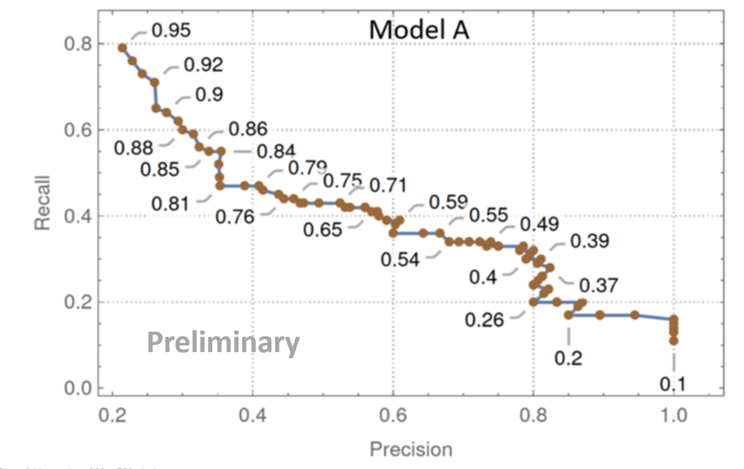
(a) Model A.

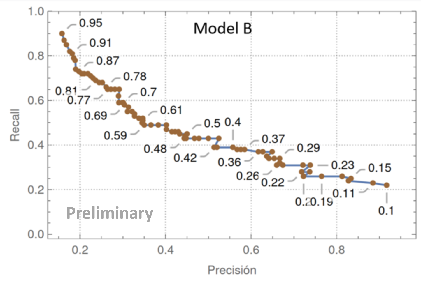
(b) Model B.

Figure 4: Precision vs recall for both models.

1.2 CNN: Object Detection

Object detection is a task based on image classification. Systems not only need to identify which category the input image belongs to, but also need to mark it with a bounding box. In the following sections we describe our implementation of object detection network for track finding.

1.2.1 Network architecture

The API (Application Programming Interface) is a framework open-source code built on TensorFlow that facilitates the construction, training and implementation of object detection models. In this interface there are a collection of detection models pre-trained on the COCO 2017 dataset, which are referred as a model zoo [8]. In this work, we use one of these models, the faster_rcnn_resnet101_coco. This network has a speed of 106 ms and a mean average precision (mAP) of 32 [9].

1.2.2 Dataset

For training data, we used 2866 tracks images and 2860 air shower images. The tracks images were obtained from simulations of horizontal muons with an energy of 100 GeV, and the air showers images were selected from the training data of model A. Also, we added one file for each image that containing the position of the vertices of the rectangle that enclosed the object that we wanted to detect. For test data, we use the same images as in the previous network (model A).

1.2.3 Results

The output for this type of network is an image with a region containing the detected object. An example is shown in figure 5. In this figure, the blue box indicates an air shower detection, and the green box indicates a track detection. In addition, each of these rectangles contains a reliability percentage. If we have a high percentage, then the detection and classification of the object is more likely to be correct. We use a 99% of this percentage to avoid false positives.

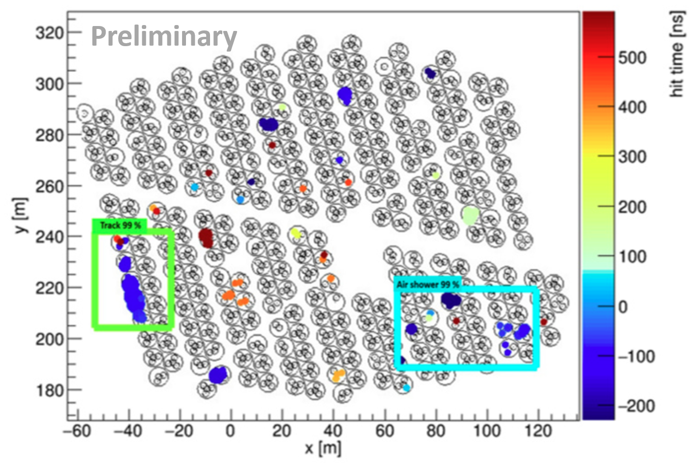
Figure 5: Output image for the CNN focused on object detection.

On the other hand, the loss function for this network is shown in the figure 6. The value of this function decreases with increasing training steps. The clearest line is the cost value, and we get the highlighted line after applying a smoothing function to these values. This function is called an exponential moving average and we use it to get a better visualization of the loss.

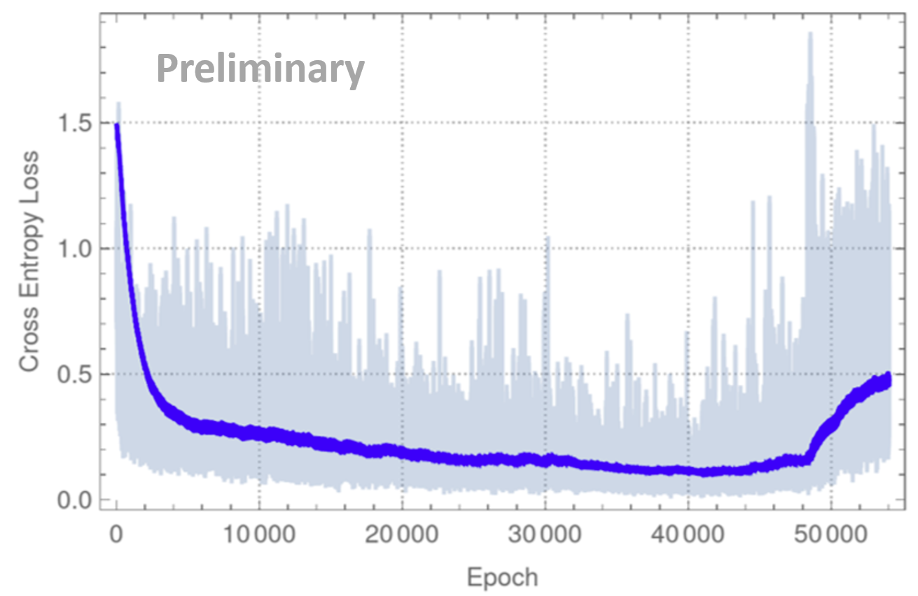
Figure 6: Loss function for the CNN focused on object detection.

2 Model Comparison

After analyzing the test dataset, in table 1, we show the threshold value or reliability percentage for which we obtained the highest value for precision variable. In this case, the network focused on object detection and model A obtained the highest value for precision, and these did not have any false positives. On the other hand, model B identified a greater number of tracks, since it obtained the highest value for recall.

Model	Threshold	%
		Precision	Recall	False positives
A	0.1	100	11	0
B	0.1	91	22	0.2
Object detection	99 %	100	11	0

Table 1: Threshold value with greater precision for the three models.

Using these threshold values, we analyze a real data set. This set consists of 118476 candidates given by the tracking algorithm. First, we apply the $\beta$ selection cut to these candidates and we had a total of 10668 events as a result. Then, we identify horizontal tracks in these events using our neural networks, the results are shown in table 2.

Model	Tracks identified	False positives
A	103	3
B	125	5
Object detection	92	0
Filtering of candidate tracks	9	0

Table 2: Comparison of tracks identified by all models for the same set of real data.

This table also shows the number of tracks identified by the third step of the algorithm mentioned in [4]. All our neural networks had an increase of an order of magnitude in the number of tracks identified compared to the previous algorithm. Also model B had the highest number of tracks identified, so in this case using a cleaner image improves the detection process, but it had the highest number of false positives. However, the object detection network did not have false positives.

3 Summary

We proposed a modification to the algorithm mentioned in [4]. This modification consisted on using convolutional neural networks. We obtained preliminary results that indicate an increase in the number of tracks identified. Here, we could see that a model with a clearer image obtains the highest number of detections, however, the network specialized in object detection does not have false positives. This is a great advantage because no other algorithm would be necessary to eliminate this contamination of events caused by false positives.

Full Authors List:  Collaboration

A.U. Abeysekara⁴⁸, A. Albert²¹, R. Alfaro¹⁴, C. Alvarez⁴¹, J.D. Álvarez⁴⁰, J.R. Angeles Camacho¹⁴, J.C. Arteaga-Velázquez⁴⁰, K. P. Arunbabu¹⁷, D. Avila Rojas¹⁴, H.A. Ayala Solares²⁸, R. Babu²⁵, V. Baghmanyan¹⁵, A.S. Barber⁴⁸, J. Becerra Gonzalez¹¹, E. Belmont-Moreno¹⁴, S.Y. BenZvi²⁹, D. Berley³⁹, C. Brisbois³⁹, K.S. Caballero-Mora⁴¹, T. Capistrán¹², A. Carramiñana¹⁸, S. Casanova¹⁵, O. Chaparro-Amaro³, U. Cotti⁴⁰, J. Cotzomi⁸, S. Coutiño de León¹⁸, E. De la Fuente⁴⁶, C. de León⁴⁰, L. Diaz-Cruz⁸, R. Diaz Hernandez¹⁸, J.C. Díaz-Vélez⁴⁶, B.L. Dingus²¹, M. Durocher²¹, M.A. DuVernois⁴⁵, R.W. Ellsworth³⁹, K. Engel³⁹, C. Espinoza¹⁴, K.L. Fan³⁹, K. Fang⁴⁵, M. Fernández Alonso²⁸, B. Fick²⁵, H. Fleischhack^51,11,52, J.L. Flores⁴⁶, N.I. Fraija¹², D. Garcia¹⁴, J.A. García-González²⁰, J. L. García-Luna⁴⁶, G. García-Torales⁴⁶, F. Garfias¹², G. Giacinti²², H. Goksu²², M.M. González¹², J.A. Goodman³⁹, J.P. Harding²¹, S. Hernandez¹⁴, I. Herzog²⁵, J. Hinton²², B. Hona⁴⁸, D. Huang²⁵, F. Hueyotl-Zahuantitla⁴¹, C.M. Hui²³, B. Humensky³⁹, P. Hüntemeyer²⁵, A. Iriarte¹², A. Jardin-Blicq^22,49,50, H. Jhee⁴³, V. Joshi⁷, D. Kieda⁴⁸, G J. Kunde²¹, S. Kunwar²², A. Lara¹⁷, J. Lee⁴³, W.H. Lee¹², D. Lennarz⁹, H. León Vargas¹⁴, J. Linnemann²⁴, A.L. Longinotti¹², R. López-Coto¹⁹, G. Luis-Raya⁴⁴, J. Lundeen²⁴, K. Malone²¹, V. Marandon²², O. Martinez⁸, I. Martinez-Castellanos³⁹, H. Martínez-Huerta³⁸, J. Martínez-Castro³, J.A.J. Matthews⁴², J. McEnery¹¹, P. Miranda-Romagnoli³⁴, J.A. Morales-Soto⁴⁰, E. Moreno⁸, M. Mostafá²⁸, A. Nayerhoda¹⁵, L. Nellen¹³, M. Newbold⁴⁸, M.U. Nisa²⁴, R. Noriega-Papaqui³⁴, L. Olivera-Nieto²², N. Omodei³², A. Peisker²⁴, Y. Pérez Araujo¹², E.G. Pérez-Pérez⁴⁴, C.D. Rho⁴³, C. Rivière³⁹, D. Rosa-Gonzalez¹⁸, E. Ruiz-Velasco²², J. Ryan²⁶, H. Salazar⁸, F. Salesa Greus^15,53, A. Sandoval¹⁴, M. Schneider³⁹, H. Schoorlemmer²², J. Serna-Franco¹⁴, G. Sinnis²¹, A.J. Smith³⁹, R.W. Springer⁴⁸, P. Surajbali²², I. Taboada⁹, M. Tanner²⁸, K. Tollefson²⁴, I. Torres¹⁸, R. Torres-Escobedo³⁰, R. Turner²⁵, F. Ureña-Mena¹⁸, L. Villaseñor⁸, X. Wang²⁵, I.J. Watson⁴³, T. Weisgarber⁴⁵, F. Werner²², E. Willox³⁹, J. Wood²³, G.B. Yodh³⁵, A. Zepeda⁴, H. Zhou³⁰

¹Barnard College, New York, NY, USA, ²Department of Chemistry and Physics, California University of Pennsylvania, California, PA, USA, ³Centro de Investigación en Computación, Instituto Politécnico Nacional, Ciudad de México, México, ⁴Physics Department, Centro de Investigación y de Estudios Avanzados del IPN, Ciudad de México, México, ⁵Colorado State University, Physics Dept., Fort Collins, CO, USA, ⁶DCI-UDG, Leon, Gto, México, ⁷Erlangen Centre for Astroparticle Physics, Friedrich Alexander Universität, Erlangen, BY, Germany, ⁸Facultad de Ciencias Físico Matemáticas, Benemérita Universidad Autónoma de Puebla, Puebla, México, ⁹School of Physics and Center for Relativistic Astrophysics, Georgia Institute of Technology, Atlanta, GA, USA, ¹⁰School of Physics Astronomy and Computational Sciences, George Mason University, Fairfax, VA, USA, ¹¹NASA Goddard Space Flight Center, Greenbelt, MD, USA, ¹²Instituto de Astronomía, Universidad Nacional Autónoma de México, Ciudad de México, México, ¹³Instituto de Ciencias Nucleares, Universidad Nacional Autónoma de México, Ciudad de México, México, ¹⁴Instituto de Física, Universidad Nacional Autónoma de México, Ciudad de México, México, ¹⁵Institute of Nuclear Physics, Polish Academy of Sciences, Krakow, Poland, ¹⁶Instituto de Física de São Carlos, Universidade de São Paulo, São Carlos, SP, Brasil, ¹⁷Instituto de Geofísica, Universidad Nacional Autónoma de México, Ciudad de México, México, ¹⁸Instituto Nacional de Astrofísica, Óptica y Electrónica, Tonantzintla, Puebla, México, ¹⁹INFN Padova, Padova, Italy, ²⁰Tecnologico de Monterrey, Escuela de Ingeniería y Ciencias, Ave. Eugenio Garza Sada 2501, Monterrey, N.L., 64849, México, ²¹Physics Division, Los Alamos National Laboratory, Los Alamos, NM, USA, ²²Max-Planck Institute for Nuclear Physics, Heidelberg, Germany, ²³NASA Marshall Space Flight Center, Astrophysics Office, Huntsville, AL, USA, ²⁴Department of Physics and Astronomy, Michigan State University, East Lansing, MI, USA, ²⁵Department of Physics, Michigan Technological University, Houghton, MI, USA, ²⁶Space Science Center, University of New Hampshire, Durham, NH, USA, ²⁷The Ohio State University at Lima, Lima, OH, USA, ²⁸Department of Physics, Pennsylvania State University, University Park, PA, USA, ²⁹Department of Physics and Astronomy, University of Rochester, Rochester, NY, USA, ³⁰Tsung-Dao Lee Institute and School of Physics and Astronomy, Shanghai Jiao Tong University, Shanghai, China, ³¹Sungkyunkwan University, Gyeonggi, Rep. of Korea, ³²Stanford University, Stanford, CA, USA, ³³Department of Physics and Astronomy, University of Alabama, Tuscaloosa, AL, USA, ³⁴Universidad Autónoma del Estado de Hidalgo, Pachuca, Hgo., México, ³⁵Department of Physics and Astronomy, University of California, Irvine, Irvine, CA, USA, ³⁶Santa Cruz Institute for Particle Physics, University of California, Santa Cruz, Santa Cruz, CA, USA, ³⁷Universidad de Costa Rica, San José , Costa Rica, ³⁸Department of Physics and Mathematics, Universidad de Monterrey, San Pedro Garza García, N.L., México, ³⁹Department of Physics, University of Maryland, College Park, MD, USA, ⁴⁰Instituto de Física y Matemáticas, Universidad Michoacana de San Nicolás de Hidalgo, Morelia, Michoacán, México, ⁴¹FCFM-MCTP, Universidad Autónoma de Chiapas, Tuxtla Gutiérrez, Chiapas, México, ⁴²Department of Physics and Astronomy, University of New Mexico, Albuquerque, NM, USA, ⁴³University of Seoul, Seoul, Rep. of Korea, ⁴⁴Universidad Politécnica de Pachuca, Pachuca, Hgo, México, ⁴⁵Department of Physics, University of Wisconsin-Madison, Madison, WI, USA, ⁴⁶CUCEI, CUCEA, Universidad de Guadalajara, Guadalajara, Jalisco, México, ⁴⁷Universität Würzburg, Institute for Theoretical Physics and Astrophysics, Würzburg, Germany, ⁴⁸Department of Physics and Astronomy, University of Utah, Salt Lake City, UT, USA, ⁴⁹Department of Physics, Faculty of Science, Chulalongkorn University, Pathumwan, Bangkok 10330, Thailand, ⁵⁰National Astronomical Research Institute of Thailand (Public Organization), Don Kaeo, MaeRim, Chiang Mai 50180, Thailand, ⁵¹Department of Physics, Catholic University of America, Washington, DC, USA, ⁵²Center for Research and Exploration in Space Science and Technology, NASA/GSFC, Greenbelt, MD, USA, ⁵³Instituto de Física Corpuscular, CSIC, Universitat de València, Paterna, Valencia, Spain

References

- [1] A. U. Abeysekara et al. (HAWC Collaboration), Observation of the Crab Nebula with the HAWC Gamma-Ray Observatory, The Astrophysical Journal 843:39, (2017) [arXiv:1701.01778].
- [2] Arun Babu K. P. et al. (HAWC Collaboration), 3HWC: The Third HAWC Catalog of Very-High-Energy Gamma-ray Sources, The Astrophysical Journal 905 (2020) 1, 76 [arXiv:2007.08582v2].
- [3] H. León Vargas, A. Sandoval, E. Belmont and R. Alfaro, Capability of the HAWC Gamma-Ray Observatory for the Indirect Detection of Ultrahigh-Energy Neutrinos, Advances in Astronomy (2017) 1932413 [arXiv:1610.04820].
- [4] H. León Vargas. Prospects of Earth-skimming neutrino detection with HAWC, in proceedings of 36th International Cosmic Ray Conference. (2019). [arXiv:1908.07622v1].
- [5] The NEXT collaboration., Kekic, M., Adams, C. et al. Demonstration of background rejection using deep convolutional neural networks in the NEXT experiment, Journal of High Energy Physics 2021, 189 (2021). https://doi.org/10.1007/JHEP01(2021)189
- [6] Ayyar, Venkitesh et al. The use of Convolutional Neural Networks for signal-background classification in Particle Physics experiments, 24th International Conference on Computing in High Energy and Nuclear Physics (CHEP2019). [arXiv:2002.05761]
- [7] Karen Simonyan and Andrew Zisserman Very Deep Convolutional Networks for Large-Scale Image Recognition, The 3rd International Conference on Learning Representations (ICLR2015). [arXiv:1409.1556]
-
[8]
“Tensorflow detection model zoo,” Last viewed: 2021-06-10. [Online]. Available: https://github.com/tensorflow/models/blob/master/research/object_detection/g3doc/tf2_detec
tion_ zoo.md - [9] J. J. Yebes, D. Montero and I. Arriola, "Learning to Automatically Catch Potholes in Worldwide Road Scene Images," in IEEE Intelligent Transportation Systems Magazine, doi: 10.1109/MITS.2019.2926370.