Further study of $f_{0}(1710)$ with coupled-channel approach and hadron molecular picture

Abstract

The $f_{0}(1710)$ was previously proposed to be dynamically generated state by interactions between vector mesons. We extend the study of $f_{0}(1710)$ by including its coupling to channels of pseudoscalar mesons within coupled-channel approach. The channels involved are $K^{*}\bar{K}^{*},\rho\rho,\omega\omega,\phi\phi,\omega\phi,\pi\pi,K\bar{K},\eta\eta$. We show that the pole assigned to $f_{0}(1710)$ does not change much. Then we calculate the partial decay widths of $f_{0}(1710)\to K^{*}\bar{K}^{*}\to\pi\pi,K\bar{K},\eta\eta$ as the coupled channel dynamically generated state as well as assuming it to be pure $K^{*}\bar{K}^{*}$ molecule. In both cases the ratios of partial decay widths agree fairly with that in PDG.

1 Introduction

More and more hadron resonances have been proposed to be hadron molecules [1] with much more predicted ones to be searched for [2]. Among various approaches for studying hadron molecules, a quite popular one is the unitary extension of chiral perturbation theory, which has been successfully to study the meson-baryon and meson-meson interactions at low energy [3, 4, 5, 6, 7, 8, 9, 10]. A well-known example is the $\Lambda(1405)$ [11], which can be dynamically generated in the vicinity of the $\pi\Sigma$ and $K^{-}p$ thresholds. The another example is $f_{0}(980)$ [8, 12], which is considered to arise due to $\pi\pi$ and $K\bar{K}$ coupled channel interaction. Some recent works [13, 14] studied the interaction of the nonet of vector mesons themselves and found a pole with quantum number $J^{PC}=0^{++}$ mainly coupling to $\bar{K}^{*}K^{*}$ channel, possibly corresponding to $f_{0}(1710)$.

In this paper, we extend the previous study [14] of $f_{0}(1710)$ by including its coupling to channels of pseudoscalar mesons in addition to vector mesons to see how these more coupled channels influence the result on the $f_{0}(1710)$ pole and meanwhile whether its corresponding partial decay widths to these channels of pseudoscalar mesons compatible with experimental data. Our work is organized as follows. In Sect. 2, we outline the formalism to the coupled-channel interaction [15]. In Sect. 3, we give our numerical results and discussion with a brief summary at the end.

2 Formalism

The interaction Lagrangian among vector mesons and pseudoscalar mesons is given by  [16, 17]

$$\mathcal{L}_{VPP}=-ig\langle V^{\mu}[P,\partial_{\mu}P]\rangle.$$ (1)

where the symbol $\langle\ldots\rangle$ stands for the trace in the $SU(3)$ space and the coupling constant $g=M_{V}/2f_{\pi}$ with $f_{\pi}=92MeV$ the pion decay constant. The vector field $V^{\mu}$ is

$$V^{\mu}=\left(\begin{array}[]{ccc}\frac{1}{\sqrt{2}}\rho^{0}+\frac{1}{\sqrt{2}}\omega&\rho^{+}&K^{*+}\\ \rho^{-}&-\frac{1}{\sqrt{2}}\rho^{0}+\frac{1}{\sqrt{2}}\omega&K^{*0}\\ K^{*-}&\bar{K}^{*0}&\phi\\ \end{array}\right)^{\mu},$$ (2)

and the pseudoscalar field $P$ is

$$P=\left(\begin{array}[]{ccc}\frac{1}{\sqrt{2}}\pi^{0}+\frac{1}{\sqrt{6}}\eta&\pi^{+}&K^{+}\\ \pi^{-}&-\frac{1}{\sqrt{2}}\pi^{0}+\frac{1}{\sqrt{6}}\eta&K^{0}\\ K^{-}&\bar{K}^{0}&-\frac{2}{\sqrt{6}}\eta\\ \end{array}\right).$$ (3)

With the Lagrangian given in Eq. (1), we are able to calculate the vector-vector to pseudoscalar-pseudoscalar scattering amplitudes. The Feynman diagrams needed are shown in Fig. 1.

Figure 1: The $t$- and $u$-channel Feynman diagrams

The amplitudes with isospin-$0$ for the processes $V(p_{1})V(p_{2})\to P(p_{3})P(p_{4})$ are listed in Table 1.

$$\begin{array}[]{cc}\hline\cr\text{Channel}&T^{(0)}\\ \hline\cr\rho\rho\xrightarrow{\pi}\pi\pi&-16(V^{\pi}_{t}+V^{\pi}_{u})\\ \rho\rho\xrightarrow{K}K\bar{K}&-2\sqrt{6}(V^{K}_{t}+V^{K}_{u})\\ \omega\omega\xrightarrow{K}K\bar{K}&2\sqrt{2}(V^{K}_{t}+V^{K}_{u})\\ \phi\phi\xrightarrow{K}K\bar{K}&4\sqrt{2}(V^{K}_{t}+V^{K}_{u})\\ \omega\phi\xrightarrow{K}K\bar{K}&-4(V^{K}_{t}+V^{K}_{u})\\ K^{*}\bar{K}^{*}\xrightarrow{K}\pi\pi&-2\sqrt{6}(V^{K}_{t}+V^{K}_{u})\\ K^{*}\bar{K}^{*}\xrightarrow{K}\eta\eta&6\sqrt{2}(V^{K}_{t}+V^{K}_{u})\\ K^{*}\bar{K}^{*}\xrightarrow{\pi,\eta}K\bar{K}&-6(V^{\pi}_{t}+V^{\eta}_{t})\\ \hline\cr\end{array}$$

Table 1: The potential of each channel with isospin-$0$

The convention used to relate the particle basis to the isospin basis is

$$\begin{split}|\pi^{+}\rangle&=-|1,1\rangle\qquad|K^{+}\rangle=-|\frac{1}{2},\frac{1}{2}\rangle,\\ |\rho^{+}\rangle&=-|1,1\rangle\qquad|K^{*+}\rangle=-|\frac{1}{2},\frac{1}{2}\rangle.\end{split}$$ (4)

The $V_{t}$ and $V_{u}$ correspond to the $t$- and $u$-channel diagrams, respectively. The superscript is the particle exchanged. Here, $t=(p_{1}-p_{3})^{2}$ and $u=(p_{1}-p_{4})^{2}$ are the usual Mandelstam variables. The potential has the form

$$V_{t(u)}^{ex}=\frac{g^{2}}{t(u)-m^{2}_{ex}}\epsilon_{1}\cdot p_{3}\epsilon_{2}\cdot p_{4}.$$ (5)

where the $\epsilon_{i}$ is the $i$-th polarization vector of the incoming vector meson. The polarization vector can be characterized by its three-momentum $\mathbf{p}_{i}$ and the third component of the spin in its rest frame, and the explicit expression of the polarization vectors can be found in Appendix A of Ref. [18].

In term of these amplitudes with isospin-$0$, we can get the $S$-wave potential via [18]

$$\begin{split}T^{(JI)}_{\ell S;\bar{\ell}\bar{S}}(s)&=\frac{Y^{0}_{\bar{\ell}}(\hat{\mathbf{z}})}{\sqrt{2}^{N}(2J+1)}\sum_{\begin{subarray}{c}\sigma_{1},\sigma_{2},\bar{\sigma}_{1}\\ \bar{\sigma}_{2},m\end{subarray}}\int\mathrm{d}\hat{\mathbf{p}}^{\prime\prime}Y^{m}_{\ell}(\mathbf{p}^{\prime\prime})^{*}(\sigma_{1}\sigma_{2}M|s_{1}s_{2}S)\\ &\times(mM\bar{M}|\ell SJ)(\bar{\sigma}_{1}\bar{\sigma}_{2}\bar{M}|\bar{s}_{1}\bar{s}_{2}\bar{S})(0\bar{M}\bar{M}|\bar{\ell}\bar{S}J)\\ &\times T^{(I)}(p_{1},p_{2},p_{3},p_{4};\epsilon_{1},\epsilon_{2},\epsilon_{3},\epsilon_{4}).\end{split}$$ (6)

with $s=(p_{1}+p_{2})^{2}$ the usual Mandelstam variable, $M=\sigma_{1}+\sigma_{2}$ and $\bar{M}=\bar{\sigma}_{1}+\bar{\sigma}_{2}$. And $N$ accounts for the identical particles, for example

$$N =2\text{ for }\rho\rho\to\pi\pi,$$ (7)

$$N =1\text{ for }\rho\rho\to K\bar{K},$$ (8)

$$N =0\text{ for }\omega\phi\to K\bar{K}.$$ (9)

Like vector scattering $VV\to VV$, the partial wave projection Eq. (6) for a $t$-channel exchange amplitude of $VV\to PP$ would also develop a left-hand cut via [14]

$$\begin{split}\frac{1}{2}&\int_{-1}^{+1}\mathrm{d}\cos\theta\frac{1}{t-m^{2}_{ex}+i\epsilon}=-\frac{s}{\sqrt{\lambda(s,m_{1}^{2},m_{2}^{2})\lambda(s,m_{3}^{2},m_{4}^{2})}}\\ &\times\log\frac{m_{1}^{2}+m_{2}^{2}-\frac{(s+m_{1}^{2}-m_{2}^{2})(s+m_{3}^{2}-m_{4}^{2})}{2s}-\frac{\sqrt{\lambda(s,m_{1}^{2},m_{2}^{2})\lambda(s,m_{3}^{2},m_{4}^{2})}}{2s}-m_{ex}^{2}+i\epsilon}{m_{1}^{2}+m_{2}^{2}-\frac{(s+m_{1}^{2}-m_{2}^{2})(s+m_{3}^{2}-m_{4}^{2})}{2s}+\frac{\sqrt{\lambda(s,m_{1}^{2},m_{2}^{2})\lambda(s,m_{3}^{2},m_{4}^{2})}}{2s}-m_{ex}^{2}+i\epsilon}.\end{split}$$ (10)

with $\lambda(a,b,c)=a^{2}+b^{2}+c^{2}-2ab-2bc-2ac$ the Källén function. In vector scattering $VV\to VV$, left-hand cuts are smoothed by the $N/D$ method [19, 20]. As for the scattering $VV\to PP$, all left-hand cuts are located below the $PP$ threshold, which are far away from the energy region we are interested in, so we do not deal with these cuts.

The basic equation to obtain the unitarized $T$-matrix is

$$T^{(JI)}(s)=\left[1-V^{(JI)}(s)\cdot G(s)\right]^{-1}\cdot V^{(JI)}(s).$$ (11)

Here $V^{(JI)}$ denotes the partial-wave amplitudes and $G(s)$ is a diagonal matrix made up by the two-point loop function $g_{i}(s)$,

$$g_{i}(s)\to i\int\frac{\mathrm{d}^{4}q}{(2\pi)^{4}}\frac{1}{(q^{2}-m^{2}_{i1}+i\epsilon)((P-q)^{2}-m^{2}_{i2}+i\epsilon)}.$$ (12)

with $P^{2}=s$ and $m_{i1,2}$ the masses of the particles in the $i$-th channel. The pole position is at the zeros of determinant

$$\text{Det}\equiv\text{det}\left[1-V^{(JI)}(s)\cdot G(s)\right].$$ (13)

The above loop function is logarithmically divergent and can be calculated with a once-subtracted dispersion relation or using a regularization $f_{\Lambda}(q)$

$$g_{i}(s)=i\int\frac{\mathrm{d}^{4}q}{(2\pi)^{4}}\frac{f^{2}_{\Lambda}(q)}{(q^{2}-m^{2}_{i1}+i\epsilon)((P-q)^{2}-m^{2}_{i2}+i\epsilon)}.$$ (14)

after the $q^{0}$ integration is performed by choosing the contour in the lower half of the complex plane, we get

$$g_{i}(s)=\int_{0}^{\infty}\frac{|\mathbf{q}|^{2}\mathrm{d}|\mathbf{q}|}{(2\pi)^{2}}\frac{\omega_{i1}+\omega_{i2}}{\omega_{i1}\omega_{i2}(s-(\omega_{i1}+\omega_{i2})^{2}+\mathrm{i}\epsilon)}f_{\Lambda}^{2}(|\mathbf{q}|).$$ (15)

where $\mathbf{q}$ is the three-momentum and $\omega_{i1,2}=\sqrt{\mathbf{q}^{2}+m^{2}_{i1,2}}$. In order to proceed we need to determine $f_{\Lambda}(\mathbf{q})$. There are two kinds of choices, sharp cutoff and smooth cutoff, typically:

$$f_{\Lambda}(\mathbf{q})=\left\{\begin{array}[]{l}\Theta(\Lambda^{2}-\mathbf{q}^{2})\\ \exp\left[-\frac{\mathbf{q}^{2}}{\Lambda^{2}}\right]\\ \end{array}\right.$$ (16)

In order to compare with the previous results of coupled channel approach [14], the same sharp cutoff is used in this paper when channels with pseudoscalar mesons are included in addition. To explore the position of the poles we need to take into account the analytical structure of these amplitudes in the different Riemann sheets. By denoting $q_{on}$ for the CM tri-momentum of the particles $1$ and $2$ in the $i$-th channel

$$q_{i}^{\text{on}}=\frac{\sqrt{(s-(m_{i1}-m_{i2})^{2})(s-(m_{i1}+m_{i2})^{2})}}{2\sqrt{s}}.$$ (17)

As the quantity is two-valued itself [21], we need to distinguish the two Riemann sheets of $q_{i}^{\text{on}}$ uniquely according to

$$q_{i}^{\text{on}>}=\left\{\begin{array}[]{cl}-q_{i}^{\text{on}}&\text{if }\text{Im}q_{i}^{\text{on}}<0\\ q_{i}^{\text{on}}&\text{else}\\ \end{array}\right.$$ (18)

And the analytic continuation to the second Riemann sheet is given by

$$g^{(2)}_{i}(s)=g_{i}(s)+\frac{i}{4\pi}\frac{q_{i}^{\text{on}>}}{\sqrt{s}}.$$ (19)

3 Numerical results and discussion

First we assume that $f_{0}(1710)$ is $K^{*}\bar{K}^{*}$ hadron molecule state and calculate the partial decay widths of $f_{0}(1710)\to K^{*}\bar{K}^{*}\to\pi\pi,K\bar{K},\eta\eta$ with the hadronic triangle loop approach [22, 23, 24, 25].

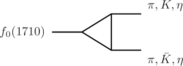
Figure 2: Decay of $f_{0}(1710)$

The loop function corresponding to this process as shown in Fig. 2 is

$$D=-i\int\frac{\mathrm{d}^{4}q}{(2\pi)^{4}}\frac{1}{(p_{3}+q)^{2}-m^{2}_{K^{*}}+i\epsilon}\frac{1}{(p_{4}-q)^{2}-m^{2}_{\bar{K}^{*}}+i\epsilon}\frac{1}{q^{2}-m^{2}_{3}+i\epsilon}.$$ (20)

where for different final state $m_{3}$ can be the mass of $\pi,K,\eta$. Since the mass of $f_{0}(1710)$ is close to the threshold of $K^{*}\bar{K}^{*}$, the internal lines with $K^{*}$ and $\bar{K}^{*}$ exchange can be approximated non-relativistically. And the the loop function can be simplified as

$$\begin{split}D&=-i\int\frac{\mathrm{d}^{4}q}{(2\pi)^{4}}\frac{1}{4m^{2}_{K^{*}}}\frac{1}{(p^{0}-\omega_{1})^{2}-(q^{0})^{2}-i\epsilon}\frac{1}{(q^{0})^{2}-\omega^{2}_{3}+i\epsilon}\\ &\times\left(\frac{\Lambda^{2}-m^{2}_{ex}}{\Lambda^{2}-q^{2}}\right)^{2}\exp\left[-\frac{(\mathbf{p}+\mathbf{q})^{2}}{\Lambda^{2}_{G}}\right].\end{split}$$ (21)

with $p_{3}=(p^{0},\mathbf{p}),q=(q^{0},\mathbf{q})$ and $\omega_{1}=\sqrt{(\mathbf{p}+\mathbf{q})^{2}+m^{2}_{K^{*}}}$, $\omega_{3}=\sqrt{\mathbf{q}^{2}+m^{2}_{3}}$. Here for the vertex $f_{0}(1710)K^{*}\bar{K}^{*}$ the Gaussian form factor is added. For the t-channel meson exchange, coupling constants with off-shell meson are dressed by monopole form factors [26, 27]. For simplicity, we take $\Lambda_{G}$ and $\Lambda$ to be equal to be in the range of $0.8\sim 1.0GeV$. And the results are

$$\frac{\Gamma(f_{0}(1710)\to\pi\pi)}{\Gamma(f_{0}(1710\to K\bar{K}))} =0.394\pm 0.134\;(0.23\pm 0.05),$$ (22)

$$\frac{\Gamma(f_{0}(1710)\to\eta\eta)}{\Gamma(f_{0}(1710\to K\bar{K}))} =0.239\pm 0.057\;(0.48\pm 0.15).$$ (23)

where the values of the PDG [28] are given between brackets. It seems that the calculated partial decay width of $f_{0}(1710)\to\pi\pi$ is larger than the central value in PDG, but it is still within the range of large error bar.

To check how the $f_{0}(1710)$ is influenced by various coupled channels in the unitary coupled channel approach, we start with the single $K^{*}\bar{K}^{*}$ channel case by dropping its couplings to all other channels. The Fig. 3 gives the $|T|^{2}$ matrix of scattering $K^{*}\bar{K}^{*}\to K^{*}\bar{K}^{*}$. We label the $K^{*}\bar{K}^{*}$ as channel $1$, and the remain channel indices are listed in Table 2. A bound state is found locating at $\sqrt{s}=1.66GeV$ for cutoff $q_{max}=0.9GeV$ and $\sqrt{s}=1.60GeV$ for $q_{max}=1.0GeV$. The bound state moves down when the cutoff $q_{max}$ increases.

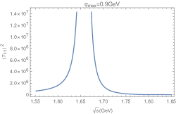
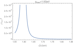
Figure 3: $|T_{11}|^{2}$ for different $q_{max}=0.9,1.0GeV$

$$\begin{array}[]{ccc}\hline\cr\text{Channel index}&\text{Channel}&\text{Threshold}~{}(GeV)\\ \hline\cr 1&K^{*}\bar{K}^{*}&1.784\\ 2&\rho\rho&1.54\\ 3&\omega\omega&1.564\\ 4&\phi\phi&2.04\\ 5&\omega\phi&1.802\\ 6&K\bar{K}&0.99\\ 7&\pi\pi&0.276\\ 8&\eta\eta&1.096\\ \hline\cr\end{array}$$

Table 2: Channel indices and threshold energies

Then we turn on additional channels to study their influence on the mass and width of the resonance. The $T$-matrix for a single channel $a$ is given by

$$T_{aa}=\frac{V_{aa}}{1-V_{aa}g_{a}}.$$ (24)

If we turn on another channel $b$, then the $T$-matrix for $a\to a$ becomes to be

$$T_{aa}=\frac{V_{aa}+\frac{V_{ab}^{2}g_{b}}{1-V_{bb}g_{b}}}{1-(V_{aa}+\frac{V_{ab}^{2}g_{b}}{1-V_{bb}g_{b}})g_{a}}.$$ (25)

Compared to the single channel, $V_{aa}$ is replaced by

$$V_{eff}=V_{aa}+\frac{V_{ab}^{2}g_{b}}{1-V_{bb}g_{b}}.$$ (26)

Denoting the second term as

$$V^{\prime}=\frac{V_{ab}^{2}g_{b}}{1-V_{bb}g_{b}},$$ (27)

then $T_{aa}$ can be written as

$$T_{aa}=\frac{V_{aa}+V^{\prime}}{1-(V_{aa}+V^{\prime})g_{a}}=\frac{(1+\alpha)V_{aa}}{1-(1+\alpha)V_{aa}g_{a}}.$$ (28)

with $\alpha=V^{\prime}/V_{aa}$. For calculating the loop integral $g_{a}$ for channels of vector mesons, we use the same sharp cutoff as in the previous study [14]. However, if we turn on the channels of pseudo-scalar mesons, such as $\eta\eta$ channel, the imaginary part of $V^{\prime}$ is too large compared with the result of triangle loop approach. In order to get consistent results with two approaches, the same kind of monopole form factor of the form

$$F=\frac{\Lambda^{2}-m^{2}_{ex}}{\Lambda^{2}-q^{2}}.$$ (29)

is needed at each $VPP$ vertex for the exchanged pseudo-scalar meson with momentum $q$. When the form factor is implemented, the $T$ matrix for $K^{*}\bar{K}^{*}\to\eta\eta$ is showed in Fig. 4.

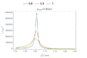
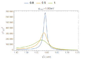
Figure 4: $|T_{18}|^{2}$ for different $\Lambda=0.8,0.9,1.0GeV$ and $q_{max}=0.9,1.0GeV$

For cutoff $q_{max}=0.9GeV$, the real part of the resonance is around $1.66GeV$, which is the same as the single channel. The imaginary part is about $6,14,26MeV$ for different $\Lambda=0.8,0.9,1.0GeV$. And for cutoff $q_{max}=1.0GeV$, the situation is similar.

For the $K^{*}\bar{K}^{*}-K\bar{K}$ system, the $|T|^{2}$ is showed in Fig. 5. The resonance is $\sqrt{s}=1.76-0.015iGeV$ for $q_{max}=0.9GeV$ and $\sqrt{s}=1.75-0.022iGeV$ for $q_{max}=1.0GeV$. Compared to the single channel, turning on the $K\bar{K}$ channel make the resonance move up along the real axis.

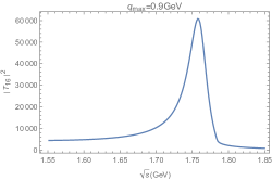
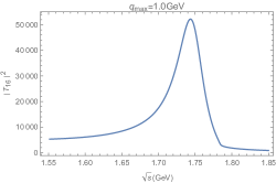
Figure 5: $|T_{16}|^{2}$ for $\Lambda=0.9GeV$ and different $q_{max}=0.9,1.0GeV$

And the situation is similar for $K^{*}\bar{K}^{*}-\pi\pi$ system, see Fig. 6.

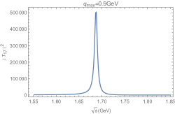
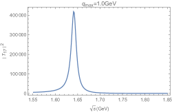
Figure 6: $|T_{17}|^{2}$ for $\Lambda=0.9GeV$ and different $q_{max}=0.9,1.0GeV$

The resonance is at $\sqrt{s}=1.69-0.004iGeV$ for $q_{max}=0.9GeV$ and $\sqrt{s}=1.64-0.007iGeV$ and $q_{max}=1.0GeV$. We find the width of the resonance in $K^{*}\bar{K}^{*}-\eta\eta$ system is about equivalence to that in $K^{*}\bar{K}^{*}-\pi\pi$ system, and about $2$~$3$ times smaller than that in $K^{*}\bar{K}^{*}-K\bar{K}$ system. For comparison, we also show the $|T|^{2}$ for $K^{*}\bar{K}^{*}-\rho\rho$ and $K^{*}\bar{K}^{*}-\omega\omega$ system, see Fig. 7.

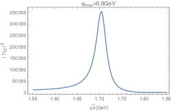
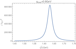
Figure 7: $|T_{12}|^{2}$ and $|T_{13}|^{2}$ for $\Lambda=0.9GeV$ and $q_{max}=0.9GeV$

The resonance is about $\sqrt{s}=1.70-0.014iGeV$ for $K^{*}\bar{K}^{*}-\rho\rho$ and $\sqrt{s}=1.63-0.013iGeV$ for $K^{*}\bar{K}^{*}-\omega\omega$ with the cutoff $q_{max}=0.9GeV$. It is interesting that turning on the $\omega\omega$ channel makes the pole to move down, recall that the pole is at $1.66GeV$ for $K^{*}\bar{K}^{*}$ single channel. Finally, we turn on all channels

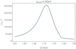
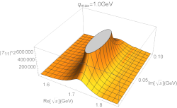
Figure 8: $|T_{11}|^{2}$ for $\Lambda=0.9GeV$ and $q_{max}=1.0GeV$ in 2-dim and 3-dim

and show the $|T_{11}|^{2}$ in 2-dim and 3-dim with $q_{max}=1.0GeV$ in Fig. 8. The position of the resonance is listed in Table 3 for different cutoffs.

$$\begin{array}[]{cccccc}\hline\cr q_{max}(GeV)&0.7&0.8&0.9&1.0&1.1\\ \hline\cr Pole(GeV)&1.77-0.015i&1.75-0.028i&1.73-0.035i&1.72-0.045i&1.70-0.053i\\ \hline\cr\end{array}$$

Table 3: The resonance pole for different cutoffs

We find that the real part of resonance is about $1710MeV$ and the width is about $100MeV$, in fairly agreement with $f_{0}(1710)$, whose mass is $1704\pm 12MeV$ and width is $123\pm 18MeV$ [28]. This means that the $f_{0}(1710)$ can be dynamically generated by mesons scattering. And we also find the lower resonance at $1.46-0.012iGeV$ for $q_{max}=1.0GeV$ and $1.48-0.008iGeV$ for $q_{max}=0.875GeV$. Compared to our previous work [29], the resonance move down a little alone the real axis, which is $1.52-0.009iGeV$ for $q_{max}=1.0GeV$ and $1.53-0.005iGeV$ for $q_{max}=0.875GeV$ in [29].

For the unitary coupled channel approach, we can calculate the ratio of decay width via [28]

$$\Gamma_{R\to a}=\frac{|\tilde{g}_{a}|^{2}}{M_{R}}\rho_{a}(M^{2}_{R}).$$ (30)

with $\tilde{g}_{a}=\mathcal{R}_{ba}/\sqrt{\mathcal{R}_{bb}}$ and $\rho_{a}$ the two-body phase space. The residues may be calculated via

$$\mathcal{R}_{ba}=-\frac{1}{2\pi i}\oint ds\mathcal{M}_{ba}.$$ (31)

The branching ratios obtained this way are

$$\frac{\Gamma(f_{0}(1710)\to\pi\pi)}{\Gamma(f_{0}(1710\to K\bar{K}))} =0.289\pm 0.092\;(0.23\pm 0.05),$$ (32)

$$\frac{\Gamma(f_{0}(1710)\to\eta\eta)}{\Gamma(f_{0}(1710\to K\bar{K}))} =0.294\pm 0.048\;(0.48\pm 0.15).$$ (33)

where the values of the PDG [28] are given in the brackets at the end of each equation for comparison. In fact the deviation from various collaborations is much larger than the PDG range: the value of $\Gamma(f_{0}(1710)\to\pi\pi)/\Gamma(f_{0}(1710\to K\bar{K}))$ is $0.64\pm 0.27\pm 0.18$ in [30], $0.41_{-0.17}^{+0.11}$ in [31], $0.2\pm 0.024\pm 0.036$ in [32], $0.39\pm 0.14$ in [33] and $0.32\pm 0.14$ in [34]. The value of $\Gamma(f_{0}(1710)\to\eta\eta)/\Gamma(f_{0}(1710\to K\bar{K}))$ is $0.48\pm 0.15$ in [35] and $0.46_{-0.38}^{+0.70}$ in [36]. And for the radiative decays of $J/\psi$ in Table 4 from PDG [28],

$$\begin{array}[]{|c|c|}\hline\cr\text{Mode}&\text{Fraction}(\Gamma_{i}/\Gamma)\\ \hline\cr\gamma f_{0}(1710)\to\gamma K\bar{K}&9.5^{+1.0}_{-0.5}\times 10^{-4}\\ \hline\cr\gamma f_{0}(1710)\to\gamma\pi\pi&3.8^{+0.5}_{-0.5}\times 10^{-4}\\ \hline\cr\gamma f_{0}(1710)\to\gamma\eta\eta&2.4^{+1.2}_{-0.7}\times 10^{-4}\\ \hline\cr\end{array}$$

Table 4: Some modes of radiative decays of $J/\psi$

all we can say is that the partial decay widths of $f_{0}(1710)\to\pi\pi$ and $f_{0}(1710)\to\eta\eta$ are similar to be around $1/3$ of $f_{0}(1710)\to K\bar{K}$, which are compatible with our results.

In summary, we extend the coupled channel interaction of nonet of vectors by including channels of the octet of pseudo-scalars in addition using the unitary coupled-channel approach. The pole near the $K^{*}\bar{K}^{*}$ threshold remains to be there with mass and width consistent with PDG values of $f_{0}(1710)$. Meanwhile we deduce the partial decay widths of $f_{0}(1710)\to K^{*}\bar{K}^{*}\to\pi\pi,K\bar{K},\eta\eta$ in the approach as well as hadronic triangle loop approach for hadronic molecule. In both cases, the results agree with that of $f_{0}(1710)$ in PDG. We can conclude that the properties of $f_{0}(1710)$ are consistent with the $K^{*}\bar{K}^{*}$ molecule state.

References

[1]
F. K. Guo, C. Hanhart, U. G. Meißner, Q. Wang, Q. Zhao and B. S. Zou,
Rev. Mod. Phys. 90, no.1, 015004 (2018)
doi:10.1103/RevModPhys.90.015004
[arXiv:1705.00141 [hep-ph]].
[2]
X. K. Dong, F. K. Guo and B. S. Zou,
Progr. Phys. 41, 65-93 (2021)
doi:10.13725/j.cnki.pip.2021.02.001
[arXiv:2101.01021 [hep-ph]].
[3]
J. Oller, E. Oset and J. Pelaez,
Phys. Rev. D 62, 114017 (2000)
doi:10.1103/PhysRevD.62.114017
[arXiv:hep-ph/9911297 [hep-ph]].
[4]
J. Oller and U. G. Meißner,
Phys. Lett. B 500, 263-272 (2001)
doi:10.1016/S0370-2693(01)00078-8
[arXiv:hep-ph/0011146 [hep-ph]].
[5]
A. Dobado and J. Pelaez,
Phys. Rev. D 56, 3057-3073 (1997)
doi:10.1103/PhysRevD.56.3057
[arXiv:hep-ph/9604416 [hep-ph]].
[6]
J. Oller and E. Oset,
Phys. Rev. D 60, 074023 (1999)
doi:10.1103/PhysRevD.60.074023
[arXiv:hep-ph/9809337 [hep-ph]].
[7]
J. Oller, E. Oset and J. Pelaez,
Phys. Rev. D 59, 074001 (1999)
doi:10.1103/PhysRevD.59.074001
[arXiv:hep-ph/9804209 [hep-ph]].
[8]
J. Oller and E. Oset,
Nucl. Phys. A 620, 438-456 (1997)
doi:10.1016/S0375-9474(97)00160-7
[arXiv:hep-ph/9702314 [hep-ph]].
[9]
J. Oller, E. Oset and A. Ramos,
Prog. Part. Nucl. Phys. 45, 157-242 (2000)
doi:10.1016/S0146-6410(00)00104-6
[arXiv:hep-ph/0002193 [hep-ph]].
[10]
R. Molina and E. Oset,
Phys. Lett. B 811, 135870 (2020)
doi:10.1016/j.physletb.2020.135870
[arXiv:2008.11171 [hep-ph]].
[11]
D. Jido, J. Oller, E. Oset, A. Ramos and U. Meissner,
Nucl. Phys. A 725, 181-200 (2003)
doi:10.1016/S0375-9474(03)01598-7
[arXiv:nucl-th/0303062 [nucl-th]].
[12]
G. Janssen, B. Pearce, K. Holinde and J. Speth,
Phys. Rev. D 52, 2690-2700 (1995)
doi:10.1103/PhysRevD.52.2690
[arXiv:nucl-th/9411021 [nucl-th]].
[13]
L. S. Geng and E. Oset,
Phys. Rev. D 79, 074009 (2009)
doi:10.1103/PhysRevD.79.074009
[arXiv:0812.1199 [hep-ph]].
[14]
M. L. Du, D. Gülmez, F. K. Guo, U. G. Meißner and Q. Wang,
Eur. Phys. J. C 78, no.12, 988 (2018)
doi:10.1140/epjc/s10052-018-6475-8
[arXiv:1808.09664 [hep-ph]].
[15]
J. A. Oller,
Prog. Part. Nucl. Phys. 110, 103728 (2020)
doi:10.1016/j.ppnp.2019.103728
[arXiv:1909.00370 [hep-ph]].
[16]
M. Bando, T. Kugo, S. Uehara, K. Yamawaki and T. Yanagida,
Phys. Rev. Lett. 54, 1215 (1985)
doi:10.1103/PhysRevLett.54.1215
[17]
M. Bando, T. Kugo and K. Yamawaki,
Phys. Rept. 164, 217-314 (1988)
doi:10.1016/0370-1573(88)90019-1
[18]
D. Gülmez, U. G. Meißner and J. Oller,
Eur. Phys. J. C 77, no.7, 460 (2017)
doi:10.1140/epjc/s10052-017-5018-z
[arXiv:1611.00168 [hep-ph]].
[19]
G. F. Chew and S. Mandelstam,
Phys. Rev. 119, 467-477 (1960)
doi:10.1103/PhysRev.119.467
[20]
J. Bjorken,
Phys. Rev. Lett. 4, 473-474 (1960)
doi:10.1103/PhysRevLett.4.473
[21]
M. Doring, C. Hanhart, F. Huang, S. Krewald and U. G. Meißner,
Nucl. Phys. A 829, 170-209 (2009)
doi:10.1016/j.nuclphysa.2009.08.010
[arXiv:0903.4337 [nucl-th]].
[22]
M. L. Du, V. Baru, F. K. Guo, C. Hanhart, U. G. Meißner, J. A. Oller and Q. Wang,
Phys. Rev. Lett. 124, no.7, 072001 (2020)
doi:10.1103/PhysRevLett.124.072001
[arXiv:1910.11846 [hep-ph]].
[23]
Y. H. Lin and B. S. Zou,
Phys. Rev. D 100, no.5, 056005 (2019)
doi:10.1103/PhysRevD.100.056005
[arXiv:1908.05309 [hep-ph]].
[24]
F. K. Guo, H. J. Jing, U. G. Meißner and S. Sakai,
Phys. Rev. D 99, no.9, 091501 (2019)
doi:10.1103/PhysRevD.99.091501
[arXiv:1903.11503 [hep-ph]].
[25]
Y. H. Lin, C. W. Shen, F. K. Guo and B. S. Zou,
Phys. Rev. D 95, no.11, 114017 (2017)
doi:10.1103/PhysRevD.95.114017
[arXiv:1703.01045 [hep-ph]].
[26]
R. Machleidt,
Adv. Nucl. Phys. 19, 189-376 (1989)
[27]
A. I. Titov, B. Kampfer and B. L. Reznik,
Eur. Phys. J. A 7, 543-557 (2000)
doi:10.1007/s100500050427
[arXiv:nucl-th/0001027 [nucl-th]].
[28]
P.A. Zyla et al. (Particle Data Group),
Prog. Theor. Exp. Phys. 2020, 083C01 (2020)
doi:10.1093/ptep/ptaa104
[29]
Z. L. Wang and B. S. Zou,
Phys. Rev. D 99, no.9, 096014 (2019)
doi:10.1103/PhysRevD.99.096014
[arXiv:1901.10169 [hep-ph]].
[30]
J. P. Lees et al. [BaBar],
Phys. Rev. D 97, no.11, 112006 (2018)
doi:10.1103/PhysRevD.97.112006
[arXiv:1804.04044 [hep-ex]].
[31]
M. Ablikim, J. Z. Bai, Y. Ban, J. G. Bian, X. Cai, H. F. Chen, H. S. Chen, H. X. Chen, J. C. Chen and J. Chen, et al.
Phys. Lett. B 642, 441-448 (2006)
doi:10.1016/j.physletb.2006.10.004
[arXiv:hep-ex/0603048 [hep-ex]].
[32]
D. Barberis et al. [WA102],
Phys. Lett. B 462, 462-470 (1999)
doi:10.1016/S0370-2693(99)00909-0
[arXiv:hep-ex/9907055 [hep-ex]].
[33]
T. A. Armstrong et al. [WA76],
Z. Phys. C 51, 351-364 (1991)
doi:10.1007/BF01548557
[34]
M. Albaladejo and J. A. Oller,
Phys. Rev. Lett. 101, 252002 (2008)
doi:10.1103/PhysRevLett.101.252002
[arXiv:0801.4929 [hep-ph]].
[35]
D. Barberis et al. [WA102],
Phys. Lett. B 479, 59-66 (2000)
doi:10.1016/S0370-2693(00)00374-9
[arXiv:hep-ex/0003033 [hep-ex]].
[36]
V. V. Anisovich, V. A. Nikonov and A. V. Sarantsev,
Phys. Atom. Nucl. 65, 1545-1552 (2002)
doi:10.1134/1.1501667
[arXiv:hep-ph/0102338 [hep-ph]].