Quotients of Probabilistic Boolean Networks

Abstract

A probabilistic Boolean network (PBN) is a discrete-time system composed of a collection of Boolean networks between which the PBN switches in a stochastic manner. This paper focuses on the study of quotients of PBNs. Given a PBN and an equivalence relation on its state set, we consider a probabilistic transition system that is generated by the PBN; the resulting quotient transition system then automatically captures the quotient behavior of this PBN. We therefore describe a method for obtaining a probabilistic Boolean system that generates the transitions of the quotient transition system. Applications of this quotient description are discussed, and it is shown that for PBNs, controller synthesis can be performed easily by first controlling a quotient system and then lifting the control law back to the original network. A biological example is given to show the usefulness of the developed results.

Probabilistic Boolean networks, probabilistic transition systems, quotienting, stabilization, optimal control.

1 Introduction

Mathematical modeling of biological systems is a valuable avenue for understanding complex biological systems and their behaviors. One powerful approach to modeling biological systems is through a Boolean model, where each system component is characterized with a binary variable. Boolean network (BN) modeling can capture the system’s behavior without the need for much kinetic detail, making it a practical choice for systems where enough kinetic information may not be at disposal [1]. A BN is typically placed in the form of a (deterministic) nonlinear system (with a finite state space); while interestingly, based on an algebraic state representation approach, the Boolean dynamics can be exactly mapped into the standard discrete-time linear dynamics [2]. This formal simplicity makes it relatively easy to formulate and solve classical control-theoretic problems for BNs, and thereby has stimulated a great many interesting subsequent developments in this area [3, 4, 5, 6, 7, 8, 9, 10, 11, 12, 13, 14, 15, 16, 17, 18, 19, 20]. For some recent work on the analysis and control of BNs based on other approaches, see, e.g., [21, 22, 23].

A probabilistic Boolean network (PBN) is a stochastic extension of the classical BN. It can be considered as a collection of BNs endowed with a probability structure describing the likelihood with which a constituent network is active. PBNs possess not only the appealing properties of BNs such as requiring few kinetic parameters, but also are able to cope with uncertainties, both in the experimental data and in the model selection [24]. The algebraic state representation has also proved a powerful framework for studying control-related problems in PBNs. Examples of recent studies based on the algebraic representation approach include investigations of network robustness and synchronization [25, 26, 27], controllability and stabilizability [28, 29, 30, 31, 32], observability and detectability [33, 34, 35], optimal control [36], just to quote a few.

It is a well-known fact that the analysis of control systems and synthesis of controllers become increasingly difficult as the dimension of the system gets larger. It is then desirable to have a methodology that reduces the size of control systems while preserving the properties relevant for analysis or synthesis. Quotient systems can be seen as lower dimensional models that may still contain enough information about the original system. A stability analysis of BNs based on a quotient map was presented in [37] and [38], where it was shown that the stability of the original BN can be inferred from the analysis of a specific quotient dynamics. Our recent work described a process for obtaining quotients of BNs [39]. A relation-based transformation strategy was introduced, which is able to transform a BN expressed in algebraic form into a quotient Boolean system suited for use. The present paper focuses on the study of quotients of PBNs. Given a PBN, together with an equivalence relation on the state set, we consider a probabilistic transition system $\mathcal{T}$ that is generated by the PBN. The equivalence relation then naturally induces a partition of the state space of $\mathcal{T}$, and the corresponding quotient system fully captures the quotient dynamics of the PBN concerned. We therefore develop a probabilistic Boolean system that produces the transitions of the quotient transition system. As an application of this quotient description, we apply the proposed technique to solve two typical control problems, namely the stabilization and optimal control problems. The results show us that through the use of an appropriately defined relation, the proposed quotient system can indeed preserve the system property relevant to control design. Consequently, synthesizing controllers for a PBN can be done easily by first designing control polices on the quotient and then inducing the control polices back to the original network.

The remainder of this paper is organized as follows. Section 2 contains the basic notation and briefly reviews PBNs and probabilistic transition systems. Section 3 details a process for generating quotients of PBNs given that the networks are represented in algebraic form. Section 4 discusses the use of the proposed quotient systems for control design and presents applications to stabilization and optimal control problems. Section 5 gives a biological example illustrating the developed results. A summary of the paper is given in the last section.

2 Notation and Preliminaries

2.1 Notation

The following notation is used throughout the paper. The symbol $\delta_{k}^{i}$ denotes the $i$th $k\times 1$ canonical basis vector (all entries of $\delta_{k}^{i}$ are $0$ except for the $i$th one, which is $1$), $\Delta_{k}$ denotes the set consisting of the canonical vectors $\delta_{k}^{1},\ldots,\delta_{k}^{k}$, and $\mathcal{L}^{k\times r}$ denotes the set of all $k\times r$ matrices whose columns are canonical basis vectors of length $k$. Elements of $\mathcal{L}^{k\times r}$ are called logical matrices (of size $k\times r$). A $(0,1)$-matrix is a matrix with all entries either $0$ or $1$. The $(i,j)$-entry of a matrix $A$ is denoted by $(A)_{ij}$. Given two $(0,1)$-matrices $A$ and $B$ of the same size, by $A\leq B$ we mean that if $(A)_{ij}=1$ then $(B)_{ij}=1$ for every $i$ and $j$. The meet of $A$ and $B$, denoted by $A\wedge B$, is the $(0,1)$-matrix whose $(i,j)$-entry is $(A)_{ij}\wedge(B)_{ij}$. The (left) semitensor product [2] of two matrices $C$ and $D$ of sizes $k_{1}\times r_{1}$ and $k_{2}\times r_{2}$, respectively, denoted by $C\ltimes D$, is defined by $C\ltimes D=(C\otimes I_{l/r_{1}})(D\otimes I_{l/k_{2}})$, where $\otimes$ is the Kronecker product of matrices, and $I_{l/r_{1}}$ and $I_{l/k_{2}}$ are the identity matrices of orders $l/r_{1}$ and $l/k_{2}$, respectively, with $l$ being the least common multiple of $r_{1}$ and $k_{2}$.

2.2 Probabilistic Boolean Networks

A PBN is described by the following stochastic equation

$$X(t+1)=f_{\theta(t)}(X(t),U(t)),$$ (1)

where $X(t)=[X_{1}(t),\ldots,X_{n}(t)]^{\top}\in\{1,0\}^{n}$ is the state, $U(t)=[U_{1}(t),\ldots,U_{m}(t)]^{\top}\in\{1,0\}^{m}$ is the control, $\{\theta(t)\colon t=0,1,\ldots\}$ is a stochastic process consisting of independent and identically distributed (i.i.d.) random variables taking values in a finite set $\mathbb{S}=\{1,\ldots,S\}$, and $f_{i}$ ($i=1,\ldots,S$) are Boolean functions from $\{1,0\}^{n+m}$ to $\{1,0\}^{n}$. By performing a matrix expression of Boolean logic and using the semitensor product, model (1) can be cast in a form similar to a random jump linear system with i.i.d. jumps. To be more precise, we let $x(t)=x_{1}(t)\ltimes\cdots\ltimes x_{n}(t)$ and $u(t)=u_{1}(t)\ltimes\cdots\ltimes u_{m}(t)$, where $x_{i}(t)=[X_{i}(t),\neg X_{i}(t)]^{\top}$ and $u_{j}(t)=[U_{j}(t),\neg U_{j}(t)]^{\top}$. Then it is shown that the PBN (1) satisfies the following algebraic description

$$x(t+1)=F_{\theta(t)}\ltimes u(t)\ltimes x(t),$$

where $x(t)\in\Delta_{N}$, $u(t)\in\Delta_{M}$, and $F_{i}\in\mathcal{L}^{N\times NM}$ for $i=1,\ldots,S$, with $N\coloneqq 2^{n}$ and $M\coloneqq 2^{m}$. For more information about obtaining the algebraic description, as well as the properties of the semitensor product, the reader is referred to, e.g., the monograph of Cheng et al. [2].

2.3 Probabilistic Transition Systems

Our discussion of quotients of PBNs will draw on the notion of probabilistic transition systems. Recall that a probability distribution over a finite set $Q$ is a function $\mu\colon Q\rightarrow[0,1]$ such that $\sum_{q\in Q}\mu(q)=1$. The set of all probability distributions over $Q$ is denoted by $\text{Dist}(Q)$. We state the following definition.

Definition 1 (see, e.g., [40, 41])

A probabilistic transition system (or probabilistic automaton) is a tuple $\mathcal{T}=(Q,Act,\rightarrow)$, where $Q$ is a finite set of states, $Act$ is a finite set of actions, and $\rightarrow\,\subseteq Q\times Act\times\text{Dist}(Q)$ is a probabilistic transition relation.

Intuitively, a transition $(q,\alpha,\mu)\in\rightarrow$ means that in the state $q$ an action $\alpha$ can be executed after which the probability to move to a state $q^{\prime}\in Q$ is $\mu(q^{\prime})$. Following standard conventions we denote $q\xrightarrow{\alpha}\mu$ if $(q,\alpha,\mu)\in\rightarrow$. A probabilistic transition system is reactive if for any state $q\in Q$ and any action $\alpha\in Act$ there exists a unique $\mu\in\text{Dist}(Q)$ such that $q\xrightarrow{\alpha}\mu$ [42]. As we will explain in the following section, every PBN corresponds naturally to a probabilistic transition system which is always reactive.

Recall that an equivalence relation $\mathcal{R}$ on $Q$ is a reflexive, symmetric, and transitive binary relation on $Q$. Let $Q/\mathcal{R}$ be the quotient set of $Q$ by $\mathcal{R}$ (i.e., the set of all equivalence classes $[q]=\{p\in Q\colon(q,p)\in\mathcal{R}\}$ for $q\in Q$). Then every $\mu\in\text{Dist}(Q)$ induces a probability distribution $\bar{\mu}$ over $Q/\mathcal{R}$ given by $\bar{\mu}([q])=\sum_{p\in[q]}\mu(p)$. The following definition of a quotient transition system is taken from [43, Definition 12], but slightly adjusted to our notation.

Definition 2

Let $\mathcal{T}=(Q,Act,\rightarrow)$ be a probabilistic transition system and let $\mathcal{R}$ be an equivalence relation on $Q$. The quotient transition system $\mathcal{T}/\mathcal{R}$ is defined by $\mathcal{T}/\mathcal{R}=(Q/\mathcal{R},Act,\rightarrow_{\mathcal{R}})$, where the probabilistic transition relation $\rightarrow_{\mathcal{R}}$ is defined as follows: for any $[q]\in Q/\mathcal{R}$ and $\pi\in\text{Dist}(Q/\mathcal{R})$, $[q]\xrightarrow{\alpha}_{\mathcal{R}}\pi$ if and only if for every $p\in[q]$ there exists a $\mu\in\text{Dist}(Q)$ inducing $\pi$ such that $p\xrightarrow{\alpha}\mu$.

It follows from the above definition that an action $\alpha$ can be executed in $[q]$ just in case: (i) $\alpha$ can be executed in every state in $[q]$, and (ii) all states in $[q]$ have identical transition probabilities to each of the equivalence classes after the action $\alpha$. Furthermore, the transition probability in $\mathcal{T}/{\mathcal{R}}$ from $[q]$ to $[q^{\prime}]$ is simply the probability with which $\mathcal{T}$ transitions from $q$ (or any other state belonging to $[q]$) to the equivalence class $[q^{\prime}]$. Note that $\mathcal{T}/\mathcal{R}$ may not be reactive even if $\mathcal{T}$ is. Indeed, it is possible that there are two states in a class, say $[q]$, which have different probabilities of transitioning to some equivalence class under a given action, say $\alpha$, thus violating the above condition (ii). Then the action $\alpha$ is not executable in $[q]$ and, consequently, the quotient transition system $\mathcal{T}/\mathcal{R}$ is not reactive.

In the next section, we will use a similar framework to study quotients of a PBN.

3 Construction of Quotients

Let us consider a PBN described by

$$\Sigma\colon\;\,x(t+1)=F_{\theta(t)}\ltimes u(t)\ltimes x(t),\;\;x\in\Delta_{N},\;\;u\in\Delta_{M}.$$ (2)

As assumed above, $\{\theta(t)\}$ is an i.i.d. process taking finitely many values $1,\ldots,S$ with associated probabilities $p_{1},\ldots,p_{S}$; and $F_{i}\in\mathcal{L}^{N\times NM}$ for each $1\leq i\leq S$. We define a column-stochastic matrix $P=p_{1}F_{1}+p_{2}F_{2}+\cdots+p_{S}F_{S}$, and for each $u\in\Delta_{M}$ let

$$P(u)=P\ltimes u.$$ (3)

The $(i,j)$-entry of $P(u)$ then gives the transition probability of $\Sigma$ from its state $\delta_{N}^{j}$ to state $\delta_{N}^{i}$ when input $u$ is applied (see, e.g., [2]). The above matrix $P$ is called the transition probability matrix of $\Sigma$ [31]. Note that any column-stochastic matrix $P$ of size $N\times NM$ can be interpreted as the transition probability matrix of a PBN of the form (2). Indeed, since every column-stochastic matrix is a convex combination of logical matrices (cf. the algorithms in [44] and [45]), there exist logical matrices $F_{1},\ldots,F_{S}$ and positive reals $\lambda_{1},\ldots,\lambda_{S}$ such that $P=\sum_{i=1}^{S}\lambda_{i}F_{i}$ and $\sum_{i=1}^{S}\lambda_{i}=1$. Let $\{\theta(t)\}$ be the i.i.d. process with the probability that $\theta(t)=i$ equal to $\lambda_{i}$ for all $t\geq 0$. Then the PBN described in (2) has as its transition probability matrix the matrix $P$.

In order to investigate quotients of (2), we first recall that every equivalence relation $\mathcal{R}\subseteq\Delta_{N}\times\Delta_{N}$ can be viewed as induced by a logical matrix $C$ with $N$ columns and full row rank, by saying

$$(x,x^{\prime})\in\mathcal{R}\Longleftrightarrow Cx=Cx^{\prime}.$$ (4)

The matrix $C$ is easily derived from the matrix representation of $\mathcal{R}$. Indeed, let $A_{\mathcal{R}}$ be the $N\times N$ matrix with entries

$$(A_{\mathcal{R}})_{ij}=\begin{cases}1&\text{if $(\delta_{N}^{i},\delta_{N}^{j})\in\mathcal{R}$},\\ 0&\text{otherwise}.\end{cases}$$

If $C$ is a matrix having the same set of distinct rows as $A_{\mathcal{R}}$, but with no rows repeated, then it must be a logical matrix of full row rank and fulfilling condition (4) (see [46, Lemma 4.6] where it is shown that such a $C$ is a logical matrix with no zero rows, hence of full row rank, and (4) holds for that $C$). Note that, for an equivalence relation $\mathcal{R}\subseteq\Delta_{N}\times\Delta_{N}$ induced by a matrix $C\in\mathcal{L}^{\widetilde{N}\times N}$ of full row rank, the quotient set $\Delta_{N}/\mathcal{R}$ has cardinality $\widetilde{N}$, and the correspondence $[x]\mapsto Cx$ gives a bijection between $\Delta_{N}/\mathcal{R}$ and $\Delta_{\widetilde{N}}$.

We now consider quotients of (2). The PBN (2) naturally generates a probabilistic transition system $\mathcal{T}(\Sigma)=(\Delta_{N},\Delta_{M},\rightarrow)$, where the transition relation $\rightarrow$ is defined as follows: for $a\in\Delta_{N}$, $u\in\Delta_{M}$, and $\mu\in\text{Dist}(\Delta_{N})$,

$$a\xrightarrow{u}\mu\Longleftrightarrow\text{$\mu(x)=x^{\top}P(u)a$ for all $x\in\Delta_{N}$}.$$

Here, $x^{\top}P(u)a$ is just the transition probability of $\Sigma$ moving from $a$ to $x$ under input $u$, since it coincides with the $(i,j)$-entry of $P(u)$ when $x=\delta_{N}^{i}$ and $a=\delta_{N}^{j}$. The above definition of $\rightarrow$ then says that, for each state $a\in\Delta_{N}$ and any $u\in\Delta_{M}$, the probability of $\mathcal{T}(\Sigma)$ transitioning to the next state $x$ is exactly the same as the probability of $\Sigma$ transitioning from $a$ to $x$. Clearly, the transition system $\mathcal{T}(\Sigma)$ generated in this way is reactive. In view of the following discussion, we mention that the converse of this fact is also true. Indeed, given a reactive transition system $\mathcal{T}^{\prime}=(\Delta_{N},\Delta_{M},\rightarrow^{\prime})$, for each $u\in\Delta_{M}$ define $P^{\prime}(u)$ to be the $N\times N$ matrix with $(i,j)$-entry $(P^{\prime}(u))_{ij}=\mu(\delta_{N}^{i})$, where $\mu$ is the unique probability distribution on $\Delta_{N}$ such that $\delta_{N}^{j}\mathrel{{\xrightarrow{u}}{}^{\prime}}\mu$. Set $P^{\prime}=$ $\left[P^{\prime}(\delta_{M}^{1})\;\cdots\;P^{\prime}(\delta_{M}^{M})\right]$. Then $P^{\prime}$ is column-stochastic (since each $P^{\prime}(u)$ is), and the system $\mathcal{T}^{\prime}$ can be considered as generated by a PBN whose transition probability matrix is $P^{\prime}$.

Let $\mathcal{R}$ be an equivalence relation on $\Delta_{N}$ and consider the quotient transition system $\mathcal{T}(\Sigma)/\mathcal{R}=(\Delta_{N}/\mathcal{R},\Delta_{M},\rightarrow_{\mathcal{R}})$. For the analysis to remain in the Boolean context, we expect that the transitions of $\mathcal{T}(\Sigma)/\mathcal{R}$ are also generated by a Boolean system of the form (2). By the above argument, this is the case exactly when $\mathcal{T}(\Sigma)/\mathcal{R}$ is reactive, or equivalently, when

$$\sum_{x\in[b]}x^{\top}P(u)a=\sum_{x\in[b]}x^{\top}P(u)a^{\prime},\;\;\forall u\in\Delta_{M},\;\forall[b]\in\Delta_{N}/\mathcal{R},\\ \text{$\forall a,a^{\prime}\in\Delta_{N}$ with $(a,a^{\prime})\in\mathcal{R}$}$$ (5)

(that is, for any control action, states in the same class have the same transition probabilities to any equivalence class). We therefore restrict our attention to those $\mathcal{R}$ satisfying (5). The following theorem gives a method for constructing a probabilistic Boolean system that generates the transitions of $\mathcal{T}(\Sigma)/\mathcal{R}$.

Theorem 1

Consider a PBN $\Sigma$ as in (2) and let $P(u)$ be as in (3). Suppose that $\mathcal{R}$ is an equivalence relation on $\Delta_{N}$ induced by a matrix $C\in\mathcal{L}^{\widetilde{N}\times N}$ of full row rank, and that property (5) holds. Let $\widetilde{C}\in\mathcal{L}^{N\times\widetilde{N}}$ be such that $\widetilde{C}\leq C^{\top}$, and for each $u\in\Delta_{M}$ define $\widetilde{P}(u)$ to be the $\widetilde{N}\times\widetilde{N}$ matrix given by $\widetilde{P}(u)=CP(u)\widetilde{C}$. Then:

1. Each $\widetilde{P}(u)$ is column-stochastic.

2. Let

   $$\Sigma_{\mathcal{R}}\colon\;x_{\mathcal{R}}(t+1)=\widetilde{F}_{\tilde{\theta}(t)}\ltimes u(t)\ltimes x_{\mathcal{R}}(t),\;\,x_{\mathcal{R}}\in\Delta_{\widetilde{N}},\;\,u\in\Delta_{M}$$

   be a probabilistic Boolean system that has $\widetilde{P}=\big{[}\widetilde{P}(\delta_{M}^{1})\;\;\widetilde{P}(\delta_{M}^{2})$ $\cdots\;\,\widetilde{P}(\delta_{M}^{M})\big{]}$ as its transition probability matrix. For any $a,a^{\prime}\in\Delta_{N}$ and any $u\in\Delta_{M}$, the transition probability of $\Sigma_{\mathcal{R}}$ from $Ca$ to $Ca^{\prime}$ under the input $u$ is equal to the transition probability of $\Sigma$ moving from $a$ to the equivalence class $[a^{\prime}]=\{x\in\Delta_{N}\colon Cx=Ca^{\prime}\}$ when $u$ is applied.

Proof 3.2.

We first claim that for all $u\in\Delta_{M}$ and $a,a^{\prime}\in\Delta_{N}$ we have

$$\sum_{x\in[a^{\prime}]}x^{\top}P(u)a=(q^{\prime})^{\top}\widetilde{P}(u)q,$$ (6)

where $q=Ca$ and $q^{\prime}=Ca^{\prime}$. To see this, suppose that $q=\delta_{\widetilde{N}}^{j}$, $q^{\prime}=\delta_{\widetilde{N}}^{i}$, and $\widetilde{C}\delta_{\widetilde{N}}^{j}=\delta_{N}^{s}$. Then

$$(q^{\prime})^{\top}\widetilde{P}(u)q =(\widetilde{P}(u))_{ij}=\sum_{l=1}^{N}\bigg{(}\sum_{k=1}^{N}(C)_{ik}(P(u))_{kl}\bigg{)}(\widetilde{C})_{lj}$$

$$=\sum_{k=1}^{N}(C)_{ik}(P(u))_{ks}.$$ (7)

The last equality follows since $(\widetilde{C})_{lj}=1$ exactly when $l=s$. Noting the equivalence

$$(C)_{ik}=1 \Longleftrightarrow C\delta_{N}^{k}=\delta_{\widetilde{N}}^{i}=q^{\prime}=Ca^{\prime}\Longleftrightarrow(\delta_{N}^{k},a^{\prime})\in\mathcal{R}$$

$$\Longleftrightarrow\delta_{N}^{k}\in[a^{\prime}],$$

we get the above (3.2) equal to

$$\sum_{\left\{k\colon\delta_{N}^{k}\in[a^{\prime}]\right\}}(P(u))_{ks}=\sum_{\delta_{N}^{k}\in[a^{\prime}]}(\delta_{N}^{k})^{\top}P(u)\delta_{N}^{s}.$$ (8)

Since $\widetilde{C}\leq C^{\top}$ and $(\widetilde{C})_{sj}=1$, we have $(C)_{js}=1$. Thus, $C\delta_{N}^{s}=\delta_{\widetilde{N}}^{j}=q=Ca$ and, hence, $(\delta_{N}^{s},a)\in\mathcal{R}$. By (5), the right-hand side of (8) is then equal to $\sum_{x\in[a^{\prime}]}x^{\top}P(u)a$, and the claim is proved.

We can now prove (a) and (b). Let $u\in\Delta_{M}$ and $1\leq j\leq\widetilde{N}$ be fixed. It follows from (6) that

$$\sum_{i=1}^{\widetilde{N}}(\widetilde{P}(u))_{ij} =\sum_{i=1}^{\widetilde{N}}(\delta_{\widetilde{N}}^{i})^{\top}\widetilde{P}(u)\delta_{\widetilde{N}}^{j}$$

$$=\sum_{i=1}^{\widetilde{N}}\sum_{\big{\{}x\colon Cx=\delta_{\widetilde{N}}^{i}\big{\}}}x^{\top}P(u)\delta_{N}^{r},$$ (9)

where $1\leq r\leq N$ is such that $C\delta_{N}^{r}=\delta_{\widetilde{N}}^{j}$ (such an $r$ exists since $C\in\mathcal{L}^{\widetilde{N}\times N}$ is of full row rank). Since $\Delta_{N}$ is the disjoint union of the sets $\big{\{}x\colon Cx=\delta_{\widetilde{N}}^{i}\big{\}}$, $i=1,\ldots,\widetilde{N}$, the above (3.2) is equal to $\sum_{k=1}^{N}(\delta_{N}^{k})^{\top}P(u)\delta_{N}^{r}=\sum_{k=1}^{N}(P(u))_{kr}=1$, where the final equality follows from the column-stochasticity of $P(u)$. This shows that $\widetilde{P}(u)$ is column-stochastic, proving (a).

In order to prove part (b), we note that the right-hand side of (6) is exactly the transition probability of $\Sigma_{\mathcal{R}}$ from $q=Ca$ to $q^{\prime}=Ca^{\prime}$ under input $u$. On the other hand, the left-hand side of (6) is the transition probability with which $\Sigma$ moves from $a$ to equivalence class $[a^{\prime}]$ when control action $u$ is applied. The assertion of part (b) then follows from (6).

Since, by the above theorem, $\Sigma_{\mathcal{R}}$ generates the transitions of $\mathcal{T}(\Sigma)/\mathcal{R}$ (recall that the assignment $[x]\mapsto Cx$ is a bijection between $\Delta_{N}/\mathcal{R}$ and $\Delta_{\widetilde{N}}$), it can be interpreted as a quotient of the PBN $\Sigma$.

Remark 3.3.

Note that for a given $u\in\Delta_{M}$, the matrix $\widetilde{P}(u)$ introduced in Theorem 1 is a constant for all $\widetilde{C}\in\mathcal{L}^{N\times\widetilde{N}}$ such that $\widetilde{C}\leq C^{\top}$. Indeed, it follows from (3.2) and (8) that the $(i,j)$-entry of $\widetilde{P}(u)$ is equal to the probability of $\Sigma$ moving from the state $\widetilde{C}\delta_{\widetilde{N}}^{j}\in\Delta_{N}$ to the equivalence class $\big{\{}x\in\Delta_{N}\colon Cx=\delta_{\widetilde{N}}^{i}\big{\}}$ when input $u$ is applied. It is easy to see that for any $\widetilde{C}\in\mathcal{L}^{N\times\widetilde{N}}$ satisfying $\widetilde{C}\leq C^{\top}$, $\widetilde{C}\delta_{\widetilde{N}}^{j}$ belongs to the equivalence class $\big{\{}x\in\Delta_{N}\colon Cx=\delta_{\widetilde{N}}^{j}\big{\}}$. Since all states in $\big{\{}x\colon Cx=\delta_{\widetilde{N}}^{j}\big{\}}$ have the same probability of transitioning into $\big{\{}x\colon Cx=\delta_{\widetilde{N}}^{i}\big{\}}$ given input $u$ (cf. (5)), the $(i,j)$-entry of $\widetilde{P}(u)$ is constant for all logical matrices $\widetilde{C}$ such that $\widetilde{C}\leq C^{\top}$, from which we conclude that $\widetilde{P}(u)$ is a constant matrix whenever $\widetilde{C}\leq C^{\top}$.

Example 3.4.

As a simple illustration of Theorem 1, consider a PBN as in (2), with $N=8$, $M=2$, and the transition probability matrix given by

$$P =\big{[}\delta_{8}^{2}\;\;0.5\delta_{8}^{1}+0.5\delta_{8}^{3}\;\;0.5\delta_{8}^{1}+0.5\delta_{8}^{3}\;\;\delta_{8}^{5}\;\;\delta_{8}^{6}\;\;\delta_{8}^{7}\;\;\delta_{8}^{8}\;\;\delta_{8}^{5}\,|$$

$$\quad\;\;\;\delta_{8}^{1}\;\;\delta_{8}^{1}\;\;\delta_{8}^{1}\;\;0.3\delta_{8}^{4}+0.7\delta_{8}^{8}\;\;\delta_{8}^{6}\;\;\delta_{8}^{7}\;\;0.5\delta_{8}^{6}+0.5\delta_{8}^{8}\;\;\delta_{8}^{7}\big{]}$$

$$=\big{[}P(\delta_{2}^{1})\;\;P(\delta_{2}^{2})\big{]}.$$

The state transition diagram of the PBN is shown in Fig. 1.

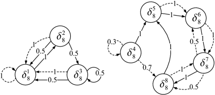
Figure 1: State transition diagram of the PBN in Example 3.4. A solid arrow represents the transition by the input $\delta_{2}^{1}$ and a dashed arrow represents the transition by the input $\delta_{2}^{2}$. The number associated with each arrow denotes the probability of the state transition given the input.

Let $\mathcal{R}$ be the equivalence relation on $\Delta_{8}$ produced by the partition $\{\{\delta_{8}^{1}\},\,\{\delta_{8}^{2},\delta_{8}^{3}\},\,\{\delta_{8}^{4}\},\,\{\delta_{8}^{5},\delta_{8}^{6},\delta_{8}^{7},\delta_{8}^{8}\}\}$ (that is, the pair $(x,x^{\prime})\in\mathcal{R}$ exactly when $x$ and $x^{\prime}$ belong to the same subset of the partition). It is easily checked that (5) is satisfied. The matrix representing $\mathcal{R}$ is

$$A_{\mathcal{R}}=\begin{bmatrix}1&0&0&0\\ 0&J_{2}&0&0\\ 0&0&1&0\\ 0&0&0&J_{4}\end{bmatrix},$$

where $J_{k}$ denotes the all-one matrix of size $k\times k$. Collapsing the identical rows of $A_{\mathcal{R}}$ yields a full row rank matrix

$$C=\big{[}\delta_{4}^{1}\;\;\delta_{4}^{2}\;\;\delta_{4}^{2}\;\;\delta_{4}^{3}\;\;\delta_{4}^{4}\;\;\delta_{4}^{4}\;\;\delta_{4}^{4}\;\;\delta_{4}^{4}\big{]}$$

which fulfills (4); and we take $\widetilde{C}=\big{[}\delta_{8}^{1}\;\;\delta_{8}^{2}\;\;\delta_{8}^{4}\;\;\delta_{8}^{5}\big{]}$, which satisfies $\widetilde{C}\leq C^{\top}$. A calculation then yields

$$\widetilde{P}(\delta_{2}^{1}) =CP(\delta_{2}^{1})\widetilde{C}=\big{[}\delta_{4}^{2}\;\;0.5\delta_{4}^{1}+0.5\delta_{4}^{2}\;\;\delta_{4}^{4}\;\;\delta_{4}^{4}\big{]},$$

$$\widetilde{P}(\delta_{2}^{2}) =CP(\delta_{2}^{2})\widetilde{C}=\big{[}\delta_{4}^{1}\;\;\delta_{4}^{1}\;\;0.3\delta_{4}^{3}+0.7\delta_{4}^{4}\;\;\delta_{4}^{4}\big{]}.$$

The state transition diagram of $\Sigma_{\mathcal{R}}$ whose transition probability matrix is given by $\widetilde{P}=\big{[}\widetilde{P}(\delta_{2}^{1})\;\;\widetilde{P}(\delta_{2}^{2})\big{]}$ is shown in Fig. 2.

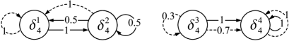
Figure 2: State transition diagram of $\Sigma_{\mathcal{R}}$ defined in Example 3.4.

It is clear from the figure that $\Sigma_{\mathcal{R}}$ is indeed a quotient of the original network which does not distinguish between states related by $\mathcal{R}$.

Theorem 1 enables us to obtain a quotient Boolean system once an equivalence relation satisfying (5) is found. For the remainder of this section, we will discuss the issue of computing equivalence relations which allow the construction of quotient Boolean systems. More precisely we consider the following problem: given a PBN $\Sigma$ and an equivalence relation $\mathcal{S}$ on $\Delta_{N}$, determine the maximal (with respect to set inclusion) equivalence relation $\mathcal{R}\subseteq\Delta_{N}\times\Delta_{N}$ such that $\mathcal{R}\subseteq\mathcal{S}$ and condition (5) holds. Here, the relation $\mathcal{S}$ may be interpreted as a preliminary classification of the states of $\Sigma$; and we focus on finding the maximal equivalence relation since in many cases we want the size of a quotient system to be as small as possible. The following theorem suggests a way of deriving such an equivalence relation.

Theorem 3.5.

Let $\Sigma$ be a PBN described by (2) and let $\mathcal{S}$ be an equivalence relation on $\Delta_{N}$. Define a sequence of relations $\mathcal{R}_{k}$ by

$$\mathcal{R}_{1}=\mathcal{S}\;\;\text{and}\;\;\mathcal{R}_{k+1}=\bigg{(}\bigcap_{u\in\Delta_{M}}\mathcal{S}_{u,k}\bigg{)}\cap\mathcal{R}_{k},$$

where $\mathcal{S}_{u,k}$ is the relation on $\Delta_{N}$ defined by: $(a,a^{\prime})\in\mathcal{S}_{u,k}$ if and only if $\sum_{x\in[b]}x^{\top}P(u)a=\sum_{x\in[b]}x^{\top}P(u)a^{\prime}$ for all $[b]\in\Delta_{N}/\mathcal{R}_{k}$, with the matrix $P(u)$ given by (3). Then:

1. The sequence of relations $\mathcal{R}_{1},\mathcal{R}_{2},\ldots,\mathcal{R}_{k},\ldots$ satisfies $\mathcal{R}_{1}\supseteq\mathcal{R}_{2}\supseteq\cdots\supseteq\mathcal{R}_{k}\supseteq\cdots$.

2. There is an integer $k^{\ast}$ such that $\mathcal{R}_{k^{\ast}+1}=\mathcal{R}_{k^{\ast}}$.

3. $\mathcal{R}_{k^{\ast}}$ is nonempty and is the maximal equivalence relation on $\Delta_{N}$ such that $\mathcal{R}_{k^{\ast}}\subseteq\mathcal{S}$ and property (5) holds.

Proof 3.6.

We first note that, since $\mathcal{R}_{1}=\mathcal{S}$ is an equivalence relation, a simple inductive argument shows that for each $k\geq 1$, $\mathcal{R}_{k}$ is also an equivalence relation and the quotient $\Delta_{N}/\mathcal{R}_{k}$ in the definition of $\mathcal{S}_{u,k}$ makes sense.

Part (a) is trivial. Part (b) follows from (a) and the finiteness of each $\mathcal{R}_{k}$. We proceed to the proof of (c). The relation $\mathcal{R}_{k^{\ast}}$ is clearly nonempty (since it contains the identity relation on $\Delta_{N}$) and is a subset of $\mathcal{S}$. To show that (5) holds true, suppose $(a,a^{\prime})\in\mathcal{R}_{k^{\ast}}$, $[b]\in\Delta_{N}/\mathcal{R}_{k^{\ast}}$ and $u\in\Delta_{M}$. Since $\mathcal{R}_{k^{\ast}}=\mathcal{R}_{k^{\ast}+1}\subseteq\mathcal{S}_{u,k^{\ast}}$, it follows, from the definition of $\mathcal{S}_{u,k^{\ast}}$, that $\sum_{x\in[b]}x^{\top}P(u)a=\sum_{x\in[b]}x^{\top}P(u)a^{\prime}$, showing that (5) holds for $\mathcal{R}_{k^{\ast}}$.

To prove the maximality of $\mathcal{R}_{k^{\ast}}$, let $\mathcal{R}\subseteq\Delta_{N}\times\Delta_{N}$ be another equivalence relation which is contained in $\mathcal{S}$ and satisfies (5). We show by induction that $\mathcal{R}\subseteq\mathcal{R}_{k}$ for all $k$. This, in particular, means that $\mathcal{R}\subseteq\mathcal{R}_{k^{\ast}}$, thus proving the maximality of $\mathcal{R}_{k^{\ast}}$. The case $k=1$ is trivial, so we take $k>1$ and assume that $\mathcal{R}\subseteq\mathcal{R}_{k-1}$. Let $(a,a^{\prime})\in\mathcal{R}$ and fix $u\in\Delta_{M}$. Then we have $\sum_{x\in E}x^{\top}P(u)a=\sum_{x\in E}x^{\top}P(u)a^{\prime}$ for any equivalence class $E$ of $\mathcal{R}$. Since $\mathcal{R}\subseteq\mathcal{R}_{k-1}$, each equivalence class in $\mathcal{R}_{k-1}$ is a disjoint union of equivalence classes of $\mathcal{R}$. It follows that $\sum_{x\in[b]}x^{\top}P(u)a=\sum_{x\in[b]}x^{\top}P(u)a^{\prime}$ for all $[b]\in\Delta_{N}/\mathcal{R}_{k-1}$, and consequently $(a,a^{\prime})\in\mathcal{S}_{u,k-1}$ by the definition of $\mathcal{S}_{u,k-1}$. Since $u\in\Delta_{M}$ is arbitrary, we have $(a,a^{\prime})\in\bigcap_{u\in\Delta_{M}}\mathcal{S}_{u,k-1}$, and noting that $(a,a^{\prime})\in\mathcal{R}\subseteq\mathcal{R}_{k-1}$ we conclude $(a,a^{\prime})\in\mathcal{R}_{k}$. This shows $\mathcal{R}\subseteq\mathcal{R}_{k}$, and the theorem is proved.

Recall that a relation $\mathcal{R}\subseteq\Delta_{N}\times\Delta_{N}$ can be represented by a $(0,1)$-matrix of size $N\times N$, whose $(i,j)$-entry is $1$ if and only if $(\delta_{N}^{i},\delta_{N}^{j})\in\mathcal{R}$. For the sake of applications, it is convenient to reformulate the above theorem in terms of $(0,1)$-matrices.

Corollary 3.7.

Suppose that $\mathcal{S}$ is an equivalence relation on $\Delta_{N}$ represented by a matrix $A_{\mathcal{S}}$. For each $u\in\Delta_{M}$ let $P(u)$ be as in (3). Define a sequence of $(0,1)$-matrices by

$$A_{1}=A_{\mathcal{S}}\;\;\text{and}\;\;A_{k+1}=A_{k}\wedge B_{k,1}\wedge\cdots\wedge B_{k,M},$$

where $B_{k,l}$ ($l=1,2,\ldots,M$) are $N\times N$ $(0,1)$-matrices whose $(i,j)$-entry is $1$ if and only if the $i$th and $j$th columns of $A_{k}P(\delta_{M}^{l})$ are identical. Then there is an integer $k^{\ast}$ such that $A_{k^{\ast}+1}=A_{k^{\ast}}$, and $A_{k^{\ast}}$ is the matrix representing the maximal equivalence relation on $\Delta_{N}$ that is contained in $\mathcal{S}$ and satisfies property (5).

Proof 3.8.

We show that, for each $k\geq 1$, the matrix $A_{k}$ represents the equivalence relation $\mathcal{R}_{k}$ defined in Theorem 3.5; the result then follows by Theorem 3.5. We proceed by induction on $k$, with the case $k=1$ being trivial. Suppose that $\mathcal{R}_{k-1}$ has the matrix representation $A_{k-1}$. For $u\in\Delta_{M}$ and $1\leq r,s\leq N$, the $(r,s)$-entry of the matrix $A_{k-1}P(u)$ is

$$\sum_{r^{\prime}=1}^{N}(A_{k-1})_{rr^{\prime}}(P(u))_{r^{\prime}s} =\sum_{r^{\prime}=1}^{N}(A_{k-1})_{rr^{\prime}}(\delta_{N}^{r^{\prime}})^{\top}P(u)\delta_{N}^{s}$$

$$=\sum_{\{r^{\prime}\colon(A_{k-1})_{rr^{\prime}}=1\}}(\delta_{N}^{r^{\prime}})^{\top}P(u)\delta_{N}^{s},$$

and since $\mathcal{R}_{k-1}$ is represented by $A_{k-1}$, this equals

$$\sum_{\{r^{\prime}:(\delta_{N}^{r},\delta_{N}^{r^{\prime}})\in\mathcal{R}_{k-1}\}}\negthickspace(\delta_{N}^{r^{\prime}})^{\top}P(u)\delta_{N}^{s}=\negthickspace\sum_{\{x:(\delta_{N}^{r},x)\in\mathcal{R}_{k-1}\}}\negthickspace x^{\top}P(u)\delta_{N}^{s}.$$

Consequently, the $i$th and $j$th columns of $A_{k-1}P(u)$ are the same exactly when

$$\sum_{\{x\colon(\delta_{N}^{r},x)\in\mathcal{R}_{k-1}\}}x^{\top}P(u)\delta_{N}^{i}=\sum_{\{x\colon(\delta_{N}^{r},x)\in\mathcal{R}_{k-1}\}}x^{\top}P(u)\delta_{N}^{j}$$

for all $1\leq r\leq N$, and the latter is clearly equivalent to saying that $\sum_{x\in[b]}x^{\top}P(u)\delta_{N}^{i}=\sum_{x\in[b]}x^{\top}P(u)\delta_{N}^{j}$ for each $[b]\in\Delta_{N}/\mathcal{R}_{k-1}$. Hence, if $\mathcal{S}_{u,k-1}$ is the relation described in Theorem 3.5 and if $u=\delta_{M}^{l}$, then

$$(\delta_{N}^{i},\delta_{N}^{j})\in\mathcal{S}_{u,k-1}\Longleftrightarrow\text{the $(i,j)$-entry of $B_{k-1,l}$ is $1$},$$

and thus $B_{k-1,l}$ is the matrix representing $\mathcal{S}_{u,k-1}$. Observe that the matrix representation of the intersection of relations is equal to the meet of the matrices representing these relations (see, e.g., [47, Section 9.3]). We conclude that the relation $\mathcal{R}_{k}$ is represented by $A_{k}$, and this completes the proof.

Example 3.9.

Consider again the PBN in Example 3.4. If we let $\mathcal{S}$ be the equivalence relation determined by the partition $\mathcal{P}=\{\{\delta_{8}^{1}\},\,\{\delta_{8}^{2},\delta_{8}^{3},\delta_{8}^{4}\},\,\{\delta_{8}^{5},\delta_{8}^{6},\delta_{8}^{7},\delta_{8}^{8}\}\}$, then

$$A_{1}=\begin{bmatrix}1&0&0\\ 0&J_{3}&0\\ 0&0&J_{4}\end{bmatrix},$$

and a direct computation from Corollary 3.7 yields

$$A_{2}=A_{3}=\begin{bmatrix}1&0&0&0\\ 0&J_{2}&0&0\\ 0&0&1&0\\ 0&0&0&J_{4}\end{bmatrix},$$

which is precisely the matrix representing the relation given in Example 3.4. Hence the relation $\mathcal{R}$ presented in Example 3.4 is the maximal equivalence relation contained in $\mathcal{S}$ which satisfies condition (5). We mention that here it is easy to check directly that the obtained $\mathcal{R}$ is indeed maximal. Specifically, note that any equivalence relation contained in $\mathcal{S}$ corresponds to a refinement of the partition $\mathcal{P}=\{\{\delta_{8}^{1}\},\,\{\delta_{8}^{2},\delta_{8}^{3},\delta_{8}^{4}\},\,\{\delta_{8}^{5},\delta_{8}^{6},\delta_{8}^{7},\delta_{8}^{8}\}\}$. Since, for $u\in\Delta_{2}$, $(\delta_{8}^{1})^{\top}P(u)\delta_{8}^{2}=(\delta_{8}^{1})^{\top}P(u)\delta_{8}^{3}\neq 0$ while $(\delta_{8}^{1})^{\top}P(u)\delta_{8}^{4}=0$, condition (5) does not hold for any equivalence relation corresponding to a refinement of $\mathcal{P}$ in which $\delta_{8}^{2}$ and $\delta_{8}^{4}$, or $\delta_{8}^{3}$ and $\delta_{8}^{4}$, belong to the same block. On the other hand, we observed in Example 3.4 that the relation $\mathcal{R}$ produced by the partition $\{\{\delta_{8}^{1}\},\,\{\delta_{8}^{2},\delta_{8}^{3}\},\,\{\delta_{8}^{4}\},\,\{\delta_{8}^{5},\delta_{8}^{6},\delta_{8}^{7},\delta_{8}^{8}\}\}$ fulfills (5); thus it is the maximal equivalence relation which is contained in $\mathcal{S}$ and satisfies (5).

To conclude, we would like to point out that the proposed method for generating a quotient of a PBN is a natural extension of the approach presented in [39] for constructing a quotient of a deterministic BN. Recall that a deterministic BN described by

$$\Sigma^{\prime}\colon\;\,x(t+1)=F\ltimes u(t)\ltimes x(t),\;x\in\Delta_{N},\;u\in\Delta_{M},\;F\in\mathcal{L}^{N\times NM}$$

can be seen as a special case of (2), with $\theta(t)$ having a constant value with probability one for all $t\geq 0$. So the results of this section apply at once. For $u\in\Delta_{M}$, let $\widetilde{F}(u)$ be defined as $\widetilde{P}(u)$ is in Theorem 1 with $P(u)$ in place of $F(u)\coloneqq F\ltimes u$. We note that $\widetilde{F}(u)$ has all nonnegative integer entries, and since it is column-stochastic by Theorem 1(a), every column contains exactly one nonzero entry and the nonzero entry equals $1$, i.e., $\widetilde{F}(u)$ is a logical matrix. Also, recall that the $(i,j)$-entry of $\widetilde{P}(u)$ defined in Theorem 1 is equal to the probability with which the original network reaches the equivalence class $\big{\{}x\in\Delta_{N}\colon Cx=\delta_{\widetilde{N}}^{i}\big{\}}$ from an arbitrary but fixed state in $\big{\{}x\colon Cx=\delta_{\widetilde{N}}^{j}\big{\}}$ when $u$ is applied (cf. Remark 3.3). Translated to the deterministic setting, this means that $(\widetilde{F}(u))_{ij}=1$ if and only if there is a one-step transition of $\Sigma^{\prime}$ from a state in $\big{\{}x\colon Cx=\delta_{\widetilde{N}}^{j}\big{\}}$ to a state in $\big{\{}x\colon Cx=\delta_{\widetilde{N}}^{i}\big{\}}$ under input $u$. The quotient system

$$x_{\mathcal{R}}(t+1)=\widetilde{F}\ltimes u(t)\ltimes x_{\mathcal{R}}(t)$$

given by Theorem 1, where $\widetilde{F}=\big{[}\widetilde{F}(\delta_{M}^{1})\;\cdots\;\widetilde{F}(\delta_{M}^{M})\big{]}$, then coincides precisely with the one presented in [39, Theorem 1], in which a state $\delta_{\widetilde{N}}^{j}$ can make a transition to another state $\delta_{\widetilde{N}}^{i}$ by applying an input exactly when that input drives $\Sigma^{\prime}$ from some state in $\big{\{}x\colon Cx=\delta_{\widetilde{N}}^{j}\big{\}}$ to some state in $\big{\{}x\colon Cx=\delta_{\widetilde{N}}^{i}\big{\}}$.

4 Control Design Via Quotients

This section illustrates the application of quotient systems for control design. We consider two typical control problems in PBNs and show how the problems can be solved through the use of a quotient Boolean system.

4.1 Stabilization

Consider a PBN $\Sigma$ as in (2) and let $P(u)$ be as in (3), which gives the (one-step) transition probabilities of $\Sigma$ under input $u\in\Delta_{M}$. A (time-invariant) feedback controller is given by a map $\mathcal{U}\colon\Delta_{N}\rightarrow\Delta_{M}$ so that if the present state is $x\in\Delta_{N}$, then the controller selects the control input $\mathcal{U}(x)\in\Delta_{M}$, resulting in the matrix $P(\mathcal{U}(x))$ that determines the one-step transition probabilities. Observe that when the present state is, say, $\delta_{N}^{i}$, only the transition probabilities of leaving $\delta_{N}^{i}$ are relevant and are given by the $i$th column of the matrix $P(\mathcal{U}(\delta_{N}^{i}))$. We use $P_{\mathcal{U}}$ to denote the matrix obtained by stacking such columns, i.e., the $i$th column of $P_{\mathcal{U}}$ is the $i$th column of $P(\mathcal{U}(\delta_{N}^{i}))$. It is easy to see that the evolution of $\Sigma$ under the control of the state feedback controller $\mathcal{U}\colon\Delta_{N}\rightarrow\Delta_{M}$ is governed by the matrix $P_{\mathcal{U}}$, i.e., the transition probability from $a\in\Delta_{N}$ to $b\in\Delta_{N}$ after $k$ steps is given by $b^{\top}P_{\mathcal{U}}^{k}a$. Let $\mathcal{M}\subseteq\Delta_{N}$ be a target set of states. The Boolean system $\Sigma$ is stabilized to $\mathcal{M}$ with probability one by $\mathcal{U}\colon\Delta_{N}\rightarrow\Delta_{M}$, if for every initial state $x_{0}\in\Delta_{N}$, there exists an integer $\tau$ such that $k\geq\tau$ implies $\sum_{x\in\mathcal{M}}x^{\top}P_{\mathcal{U}}^{k}x_{0}=1$ (see, e.g., [48, 31]). The following result shows that we can easily derive a stabilizing controller for $\Sigma$ on the basis of a stabilizing controller for its quotient system.

Proposition 4.10.

Consider a PBN $\Sigma$ as given in (2). Let $\mathcal{M}\subseteq\Delta_{N}$ and let $\mathcal{S}$ be the equivalence relation on $\Delta_{N}$ determined by the partition $\left\{\mathcal{M},\Delta_{N}-\mathcal{M}\right\}$. Suppose that $\mathcal{R}$ is an equivalence relation on $\Delta_{N}$ induced by a full row rank matrix $C\in\mathcal{L}^{\widetilde{N}\times N}$, $\mathcal{R}\subseteq\mathcal{S}$, and (5) holds. Suppose $\Sigma_{\mathcal{R}}$ is defined as in Theorem 1 and let $\mathcal{M}_{\mathcal{R}}=\{Cx\colon x\in\mathcal{M}\}$. Then:

1. There exists a control law $\mathcal{U}\colon\Delta_{N}\rightarrow\Delta_{M}$ that stabilizes $\Sigma$ to $\mathcal{M}$ with probability one if and only if there exists a control law $\mathcal{U}_{\mathcal{R}}\colon\Delta_{\widetilde{N}}\rightarrow\Delta_{M}$ that stabilizes $\Sigma_{\mathcal{R}}$ to $\mathcal{M}_{\mathcal{R}}$ with probability one.

2. If the controller $x_{\mathcal{R}}\mapsto\mathcal{U}_{\mathcal{R}}(x_{\mathcal{R}})$ stabilizes $\Sigma_{\mathcal{R}}$ to $\mathcal{M}_{\mathcal{R}}$ with probability one, then the controller given by $x\mapsto\mathcal{U}(x)=\mathcal{U}_{\mathcal{R}}(Cx)$ stabilizes $\Sigma$ to $\mathcal{M}$ with probability one.

For the proof of Proposition 4.10 we need the following lemma adapted from [49]. To make the paper self-contained, the proof of this lemma is given in the Appendix.

Lemma 4.11.

Consider a PBN as in (2). Let $\mathcal{M}\subseteq\Delta_{N}$, and let $\mathcal{M}^{\ast}$ be the last term of the sequence

$$\mathcal{M}_{0} =\mathcal{M},$$

$$\mathcal{M}_{i} =\mathcal{M}_{i-1}\cap\mathcal{A}(\mathcal{M}_{i-1}),\quad i=1,\ldots,\iota,$$

where $\mathcal{A}(\mathcal{M}_{i-1})=\{a\in\Delta_{N}\colon\sum_{x\in\mathcal{M}_{i-1}}x^{\top}P(u)a=1\>\text{for some}$ $u\in\Delta_{M}\}$, and the value of $\iota$ is determined by the condition $\mathcal{M}_{\iota+1}=\mathcal{M}_{\iota}$. Define the sequence $\mathcal{Z}_{j}$ according to

$$\mathcal{Z}_{0} =\mathcal{M}^{\ast},$$

$$\mathcal{Z}_{j} =\Big{\{}a\in\Delta_{N}:\negthickspace\sum_{x\in\mathcal{Z}_{j-1}}\negthickspace x^{\top}P(u)a=1\,\text{for}\,\text{some}\,u\in\Delta_{M}\Big{\}},\,j\geq 1.$$

Then $\mathcal{Z}_{j}\supseteq\mathcal{Z}_{j-1}$, and the PBN can be stabilized to $\mathcal{M}$ with probability one by a feedback $\mathcal{U}\colon\Delta_{N}\rightarrow\Delta_{M}$ if, and only if, $\mathcal{Z}_{\lambda}=\Delta_{N}$ for some $\lambda\geq 1$.

Proof 4.12 (Proof of Proposition 4.10).

(a) Let $\mathcal{M}_{i}$ and $\mathcal{Z}_{j}$ be as in Lemma 4.11. Let $\mathcal{M}_{\mathcal{R}}^{\ast}$ be the last term of the sequence

$$\widetilde{\mathcal{M}}_{0} =\mathcal{M}_{\mathcal{R}},$$

$$\widetilde{\mathcal{M}}_{i} =\widetilde{\mathcal{M}}_{i-1}\cap\mathcal{A}^{\prime}(\widetilde{\mathcal{M}}_{i-1}),\quad i=1,\ldots,\iota^{\prime},$$

where $\mathcal{A}^{\prime}(\widetilde{\mathcal{M}}_{i-1})=\{q\in\Delta_{\widetilde{N}}\colon\sum_{z\in\widetilde{\mathcal{M}}_{i-1}}z^{\top}\widetilde{P}(u)q=1\>\text{for some}$ $u\in\Delta_{M}\}$, and the value of $\iota^{\prime}$ is determined by the condition $\widetilde{\mathcal{M}}_{\iota^{\prime}+1}=\widetilde{\mathcal{M}}_{\iota^{\prime}}$. Define the sequence $\widetilde{\mathcal{Z}}_{j}$ according to

$$\widetilde{\mathcal{Z}}_{0} =\mathcal{M}_{\mathcal{R}}^{\ast},$$

$$\widetilde{\mathcal{Z}}_{j} =\bigg{\{}q\in\Delta_{\widetilde{N}}:\negthickspace\sum_{z\in\widetilde{\mathcal{Z}}_{j-1}}\negthickspace z^{\top}\widetilde{P}(u)q=1\,\text{for}\,\text{some}\,u\in\Delta_{M}\bigg{\}},\,j\geq 1.$$

We show that for $j\geq 0$,

$$x\in\mathcal{Z}_{j}\Longleftrightarrow Cx\in\widetilde{\mathcal{Z}}_{j}.$$ (10)

First, we claim that

$$x\in\mathcal{M}_{i}\Longleftrightarrow Cx\in\widetilde{\mathcal{M}}_{i}.$$ (11)

Indeed, if $Cx\in\widetilde{\mathcal{M}}_{0}$, then there exists $x^{\prime}\in\mathcal{M}$ such that $Cx=Cx^{\prime}$, and hence $(x,x^{\prime})\in\mathcal{R}\subseteq\mathcal{S}$, forcing $x\in\mathcal{M}$ since $\mathcal{S}$ is the equivalence relation yielded by the partition $\left\{\mathcal{M},\Delta_{N}-\mathcal{M}\right\}$. This shows that $Cx\in\widetilde{\mathcal{M}}_{0}\Rightarrow x\in\mathcal{M}_{0}$. The converse implication is trivial. Assume by induction that $x\in\mathcal{M}_{i-1}\Longleftrightarrow Cx\in\widetilde{\mathcal{M}}_{i-1}$. Denoting $I(z)=\{x\in\Delta_{N}\colon Cx=z\}$ for $z\in\Delta_{\widetilde{N}}$, which is nonempty since $C$ is supposed to have full row rank, then $\mathcal{M}_{i-1}$ can be partitioned as the disjoint union $\mathcal{M}_{i-1}=\bigcup_{z\in\widetilde{\mathcal{M}}_{i-1}}I(z)$. Indeed, the sets $I(z)$, $z\in\widetilde{\mathcal{M}}_{i-1}$, are clearly mutually disjoint, and for any $x\in\Delta_{N}$, $x\in\mathcal{M}_{i-1}$ if and only if $Cx\in\widetilde{\mathcal{M}}_{i-1}$, if and only if $x\in I(z)$ for some $z\in\widetilde{\mathcal{M}}_{i-1}$. Suppose $x\in\Delta_{N}$, $u\in\Delta_{M}$, and let $q=Cx$. Then

$$\sum_{b\in\mathcal{M}_{i-1}}b^{\top}P(u)x=\negthickspace\sum_{z\in\widetilde{\mathcal{M}}_{i-1}}\sum_{b\in I(z)}b^{\top}P(u)x=\negthickspace\sum_{z\in\widetilde{\mathcal{M}}_{i-1}}\negthickspace z^{\top}\widetilde{P}(u)q,$$

where the second equality follows from (6) in the proof of Theorem 1. This immediately implies that $x\in\mathcal{A}(\mathcal{M}_{i-1})$ if and only if $Cx\in\mathcal{A}^{\prime}(\widetilde{\mathcal{M}}_{i-1})$, and hence $x\in\mathcal{M}_{i}$ if and only if $Cx\in\widetilde{\mathcal{M}}_{i}$.

The proof of (10) is easily obtained by induction on $j$. It follows from (11) that $x\in\mathcal{Z}_{0}$ if and only if $Cx\in\widetilde{\mathcal{Z}}_{0}$, establishing the base step. The induction step is similar to that done in the proof of (11).

Since $C$ is of full row rank, we conclude from (10) that $\mathcal{Z}_{j}=\Delta_{N}$ if and only if $\widetilde{\mathcal{Z}}_{j}=\Delta_{\widetilde{N}}$, and the proof of (a) follows by Lemma 4.11.

(b) Define the matrix $\widetilde{P}_{\mathcal{U}_{\mathcal{R}}}$ for $\Sigma_{\mathcal{R}}$ in the same way as $P_{\mathcal{U}}$ is defined for $\Sigma$. We first prove that, for any $a\in\Delta_{N}$, $z\in\Delta_{\widetilde{N}}$, and integer $k\geq 1$, we have

$$\sum_{x\in I(z)}x^{\top}P_{\mathcal{U}}^{k}a=z^{\top}\widetilde{P}_{\mathcal{U}_{\mathcal{R}}}^{k}q,$$ (12)

where $I(z)=\{x\in\Delta_{N}\colon Cx=z\}$ and $q=Ca$. The proof is by induction on $k$. Since $P_{\mathcal{U}}a=P(\mathcal{U}(a))a$ by the construction of $P_{\mathcal{U}}$, it follows from (6) in the proof of Theorem 1 that

$$\sum_{x\in I(z)}x^{\top}P_{\mathcal{U}}a=\sum_{x\in I(z)}x^{\top}P(\mathcal{U}(a))a=z^{\top}\widetilde{P}(\mathcal{U}(a))q,$$

and since $\mathcal{U}(a)=\mathcal{U}_{\mathcal{R}}(Ca)=\mathcal{U}_{\mathcal{R}}(q)$, the above is equal to $z^{\top}\widetilde{P}(\mathcal{U}_{\mathcal{R}}(q))q=z^{\top}\widetilde{P}_{\mathcal{U}_{\mathcal{R}}}q$. This gives (12) for $k=1$. Assume as induction hypothesis that the statement holds for $k-1$. Decomposing the $N\times N$ identity matrix as $\sum_{b\in\Delta_{N}}bb^{\top}$, we have

$$\sum_{x\in I(z)}x^{\top}P_{\mathcal{U}}^{k}a=\sum_{x\in I(z)}x^{\top}P_{\mathcal{U}}\bigg{(}\sum_{b\in\Delta_{N}}bb^{\top}\bigg{)}P_{\mathcal{U}}^{k-1}a$$

$$\qquad=\sum_{x\in I(z)}\sum_{b\in\Delta_{N}}x^{\top}P_{\mathcal{U}}bb^{\top}P_{\mathcal{U}}^{k-1}a$$

$$\qquad=\sum_{i=1}^{\widetilde{N}}\sum_{b\in I(\delta_{\widetilde{N}}^{i})}\bigg{(}\sum_{x\in I(z)}x^{\top}P_{\mathcal{U}}b\bigg{)}b^{\top}P_{\mathcal{U}}^{k-1}a.$$ (13)

The last equality holds true since $\Delta_{N}$ is the disjoint union of the sets $I(\delta_{\widetilde{N}}^{i})=\{x\colon Cx=\delta_{\widetilde{N}}^{i}\}$, $i=1,\ldots,\widetilde{N}$. It follows from the case $k=1$ that $\sum_{x\in I(z)}x^{\top}P_{\mathcal{U}}b=z^{\top}\widetilde{P}_{\mathcal{U}_{\mathcal{R}}}\delta_{\widetilde{N}}^{i}$ for all $b\in I(\delta_{\widetilde{N}}^{i})$, and the right-hand side of (4.12) is equal to the following expression:

$$\sum_{i=1}^{\widetilde{N}}z^{\top}\widetilde{P}_{\mathcal{U}_{\mathcal{R}}}\delta_{\widetilde{N}}^{i}\bigg{(}\sum_{b\in I(\delta_{\widetilde{N}}^{i})}b^{\top}P_{\mathcal{U}}^{k-1}a\bigg{)}.$$ (14)

According to the induction hypothesis, we have for each $1\leq i\leq\widetilde{N}$,

$$\sum_{b\in I(\delta_{\widetilde{N}}^{i})}b^{\top}P_{\mathcal{U}}^{k-1}a=(\delta_{\widetilde{N}}^{i})^{\top}\widetilde{P}_{\mathcal{U}_{\mathcal{R}}}^{k-1}q,$$

and substituting this into (14) we get

$$\sum_{x\in I(z)}x^{\top}P_{\mathcal{U}}^{k}a=\sum_{i=1}^{\widetilde{N}}z^{\top}\widetilde{P}_{\mathcal{U}_{\mathcal{R}}}\delta_{\widetilde{N}}^{i}\Big{[}(\delta_{\widetilde{N}}^{i})^{\top}\widetilde{P}_{\mathcal{U}_{\mathcal{R}}}^{k-1}q\Big{]}$$

$$\qquad=z^{\top}\widetilde{P}_{\mathcal{U}_{\mathcal{R}}}\bigg{[}\sum_{i=1}^{\widetilde{N}}\delta_{\widetilde{N}}^{i}(\delta_{\widetilde{N}}^{i})^{\top}\bigg{]}\widetilde{P}_{\mathcal{U}_{\mathcal{R}}}^{k-1}q=z^{\top}\widetilde{P}_{\mathcal{U}_{\mathcal{R}}}^{k}q,$$

which is (12).

From the proof of (a), we know that $x\in\mathcal{M}$ if and only if $Cx\in\mathcal{M}_{\mathcal{R}}$, and consequently, we can write $\mathcal{M}$ as the disjoint union $\mathcal{M}=\bigcup_{z\in\mathcal{M}_{\mathcal{R}}}I(z)$. The proof of part (b) is now obvious. Suppose $x_{0}\in\Delta_{N}$. Let $x_{\mathcal{R}}^{0}=Cx_{0}$. Then for each integer $k\geq 1$ we have

$$\sum_{x\in\mathcal{M}}x^{\top}P_{\mathcal{U}}^{k}x_{0}=\sum_{z\in\mathcal{M}_{\mathcal{R}}}\sum_{x\in I(z)}x^{\top}P_{\mathcal{U}}^{k}x_{0}=\sum_{z\in\mathcal{M}_{\mathcal{R}}}z^{\top}\widetilde{P}_{\mathcal{U}_{\mathcal{R}}}^{k}x_{\mathcal{R}}^{0},$$

from which part (b) follows immediately.

4.2 Optimal Control

Let us consider the following optimal control problem, introduced in [50].

Problem 4.13.

Consider a PBN as in (2). Given an initial state $x_{0}\in\Delta_{N}$ and a finite time horizon $T\in\mathbb{Z}^{+}$, find a control policy, $u(t)=\mathcal{U}^{\ast}(t,x(t))$ for $0\leq t\leq T-1$, that minimizes the cost functional

$$J=\mathbb{E}\bigg{[}g(x(T))+\sum_{t=0}^{T-1}l(u(t),x(t))\bigg{]},$$

where $l(u,x)$ and $g(x)$ are real-valued functions defined on $\Delta_{M}\times\Delta_{N}$ and $\Delta_{N}$, respectively.

We show that the solution to Problem 4.13 can be found by considering the problem for a suitably chosen quotient system. To this end, let $\mathcal{S}$ be the equivalence relation on $\Delta_{N}$ given by

$$(x,x^{\prime})\in\mathcal{S} \Longleftrightarrow\text{$g(x)=g(x^{\prime})$ and}$$

$$\qquad\;\,\text{$l(u,x)=l(u,x^{\prime})$ for all $u\in\Delta_{M}$}.$$ (15)

We note that, if $C\in\mathcal{L}^{\widetilde{N}\times N}$ has full row rank, and if the equivalence relation $\mathcal{R}$ induced by $C$ satisfies $\mathcal{R}\subseteq\mathcal{S}$, then every $z\in\Delta_{\widetilde{N}}$ can be written as $z=Cx$ for some $x\in\Delta_{N}$ and the function $g$ is constant on the set $I(z)=\{x\in\Delta_{N}\colon Cx=z\}$. Hence, the map $g_{\mathcal{R}}\colon\Delta_{\widetilde{N}}\rightarrow\mathbb{R}$, given by

$$g_{\mathcal{R}}(z)=g_{\mathcal{R}}(Cx)=g(x),$$ (16)

is well defined. For the same reason, the map $l_{\mathcal{R}}\colon\Delta_{M}\times\Delta_{\widetilde{N}}\rightarrow\mathbb{R}$ defined by

$$l_{\mathcal{R}}(u,z)=l_{\mathcal{R}}(u,Cx)=l(u,x)$$ (17)

is also well defined. We can state the following proposition.

Proposition 4.14.

Let $\Sigma$ be a PBN described by (2) and consider Problem 4.13 with given $x_{0}$ and $T$. Suppose that $\mathcal{S}$ is the equivalence relation given by (4.2), $\mathcal{R}\subseteq\Delta_{N}\times\Delta_{N}$ is an equivalence relation induced by a full row rank matrix $C\in\mathcal{L}^{\widetilde{N}\times N}$, $\mathcal{R}\subseteq\mathcal{S}$, and (5) holds. Let $\Sigma_{\mathcal{R}}$ be the probabilistic Boolean system constructed in Theorem 1, and define $J_{\mathcal{R}}=\mathbb{E}\,\big{[}g_{\mathcal{R}}(x_{\mathcal{R}}(T))+\sum_{t=0}^{T-1}l_{\mathcal{R}}(u(t),x_{\mathcal{R}}(t))\big{]}$, where $g_{\mathcal{R}}$ and $l_{\mathcal{R}}$ are given by (16) and (17). Suppose that $(t,x_{\mathcal{R}})\mapsto\mathcal{U}_{\mathcal{R}}^{\ast}(t,x_{\mathcal{R}})$ is an optimal control policy solving Problem 4.13 with $\Sigma$, $x_{0}$, and $J$ replaced by $\Sigma_{\mathcal{R}}$, $x_{\mathcal{R}}^{0}=Cx_{0}$, and $J_{\mathcal{R}}$, respectively. Then the control policy given by $(t,x)\mapsto\mathcal{U}^{\ast}(t,x)=\mathcal{U}_{\mathcal{R}}^{\ast}(t,Cx)$ is an optimal control policy for $\Sigma$. Moreover, let $J^{\ast}$ be the optimal value of $J$ given the initial state $x_{0}$ and let $J_{\mathcal{R}}^{\ast}$ be the optimal value of $J_{\mathcal{R}}$ associated with $x_{\mathcal{R}}^{0}=Cx_{0}$. Then $J^{\ast}=J_{\mathcal{R}}^{\ast}$.

The proof of the proposition follows from the following two lemmas.

Lemma 4.15.

Consider Problem 4.13 with given $x_{0}$ and $T$. Let $\mathcal{S}$, $\mathcal{R}$, and $C$ be as in Proposition 4.14. Then there exists an optimal control policy $(t,x)\mapsto\overline{\mathcal{U}}(t,x)$ with the property that $\overline{\mathcal{U}}(t,x)=\overline{\mathcal{U}}(t,x^{\prime})$ for all $0\leq t\leq T-1$ and all $x,x^{\prime}\in\Delta_{N}$ such that $Cx=Cx^{\prime}$.

Proof 4.16.

Consider the following dynamic programming algorithm (adapted from [51, Proposition 1.3.1]; see also [50]):

$$H(T,x)=g(x),\quad x\in\Delta_{N},$$

$$H(t,x)=\min_{u\in\Delta_{M}}\bigg{\{}l(u,x)+\sum_{\xi\in\Delta_{N}}H(t+1,\xi)\xi^{\top}P(u)x\bigg{\}},$$

$$\qquad\qquad\qquad x\in\Delta_{N},\quad t=T-1,\ldots,1,0,$$

where $P(u)$ is as in (3). If we let

$$G(t,x,u)=l(u,x)+\sum_{\xi\in\Delta_{N}}H(t+1,\xi)\xi^{\top}P(u)x,$$

and define

$$\overline{\mathcal{U}}(t,x)\in\arg\min_{u\in\Delta_{M}}G(t,x,u),\;\;0\leq t\leq T-1,\;\;x\in\Delta_{N},$$

then the control law given by $(t,x)\mapsto\overline{\mathcal{U}}(t,x)$ is optimal [51, 50]. We will show that for $0\leq t\leq T-1$,

$$G(t,x,u)=G(t,x^{\prime},u),\quad\forall u\in\Delta_{M},\;\;\forall x,x^{\prime}\in\Delta_{N}\\ \text{with}\;Cx=Cx^{\prime}.$$ (18)

Then we can find $\overline{\mathcal{U}}(t,x)\in\arg\min_{u}G(t,x,u)$ with the desired property. This will prove the lemma.

Fix $u\in\Delta_{M}$ and let $x,x^{\prime}\in\Delta_{N}$ be such that $Cx=Cx^{\prime}$. Since $(x,x^{\prime})\in\mathcal{R}\subseteq\mathcal{S}$, it follows from (4.2) that

$$l(u,x)=l(u,x^{\prime}).$$ (19)

For each $z\in\Delta_{\widetilde{N}}$, since $H(T,\cdot)=g(\cdot)$ is constant on the set $I(z)=\{\xi\in\Delta_{N}\colon C\xi=z\}$ (cf. the statement following (4.2)) and since

$$\sum_{\xi\in I(z)}\xi^{\top}P(u)x=\sum_{\xi\in I(z)}\xi^{\top}P(u)x^{\prime}$$

by (5), we have

$$\sum_{\xi\in I(z)}H(T,\xi)\xi^{\top}P(u)x=\sum_{\xi\in I(z)}H(T,\xi)\xi^{\top}P(u)x^{\prime}.$$

Hence,

$$\sum_{\xi\in\Delta_{N}}H(T,\xi)\xi^{\top}P(u)x=\sum_{\xi\in\Delta_{N}}H(T,\xi)\xi^{\top}P(u)x^{\prime},$$

since $\Delta_{N}$ is the disjoint union of $I(z)$, $z\in\Delta_{\widetilde{N}}$. This together with (19) gives $G(T-1,x,u)=G(T-1,x^{\prime},u)$. Thus (18) is true if $t=T-1$.

Note that if $t\leq T-1$ and if (18) is true for $t$, then for any $\xi,\xi^{\prime}\in\Delta_{N}$ with $C\xi=C\xi^{\prime}$, we have

$$H(t,\xi)=\min_{u\in\Delta_{M}}G(t,\xi,u)=\min_{u\in\Delta_{M}}G(t,\xi^{\prime},u)=H(t,\xi^{\prime}).$$

Thus with this $t$ fixed, the function $H(t,\cdot)$ is constant on each of the sets $I(z)=\{\xi\colon C\xi=z\}$. Then by an argument similar to that in the previous paragraph, we can show that (18) is true for $t-1$ also, and so working by downward induction on $t$, we conclude that (18) holds true for all $0\leq t\leq T-1$, as required. The proof is complete.

Lemma 4.17.

Let the notation be as in the statement of Proposition 4.14. If the initial states of $\Sigma$ and $\Sigma_{\mathcal{R}}$ satisfy $Cx_{0}=x_{\mathcal{R}}^{0}$, and if the two control policies $(t,x)\mapsto\mathcal{U}(t,x)$ and $(t,x_{\mathcal{R}})\mapsto\widetilde{\mathcal{U}}(t,x_{\mathcal{R}})$ satisfy $\mathcal{U}(t,x)=\widetilde{\mathcal{U}}(t,Cx)$ for all $0\leq t\leq T-1$ and $x\in\Delta_{N}$, then the cost functionals $J$ and $J_{\mathcal{R}}$ have the same value.

Proof 4.18.

For each $0\leq t\leq T-1$, let $P_{t}$ be the matrix whose $i$th column is the $i$th column of the matrix $P(\mathcal{U}(t,\delta_{N}^{i}))$, and let $\widetilde{P}_{t}$ be the matrix in which the $j$th column is the $j$th column of $\widetilde{P}(\widetilde{\mathcal{U}}(t,\delta_{\widetilde{N}}^{j}))$. With a similar argument to that in proving (12), it is easy to see that for any $a\in\Delta_{N}$, $z\in\Delta_{\widetilde{N}}$, and $1\leq t\leq T$, we have $\sum_{x\in I(z)}x^{\top}P_{t-1}P_{t-2}\cdots P_{0}a=z^{\top}\widetilde{P}_{t-1}\widetilde{P}_{t-2}\cdots\widetilde{P}_{0}q$, where $I(z)=\{x\in\Delta_{N}\colon Cx=z\}$ and $q=Ca$. Fix $1\leq t\leq T-1$, and fix $s\in\{l(u,x)\colon(u,x)\in\Delta_{M}\times\Delta_{N}\}$. Define

$$\mathcal{M}(t,s) =\{x\in\Delta_{N}\colon l(\mathcal{U}(t,x),x)=s\},$$

$$\widetilde{\mathcal{M}}(t,s) =\{x_{\mathcal{R}}\in\Delta_{\widetilde{N}}\colon l_{\mathcal{R}}(\widetilde{\mathcal{U}}(t,x_{\mathcal{R}}),x_{\mathcal{R}})=s\}.$$

Since $l(\mathcal{U}(t,x),x)=l(\widetilde{\mathcal{U}}(t,Cx),x)=l_{\mathcal{R}}(\widetilde{\mathcal{U}}(t,Cx),Cx)$, it follows that $x\in\mathcal{M}(t,s)$ if and only if $Cx\in\widetilde{\mathcal{M}}(t,s)$, and hence $\mathcal{M}(t,s)$ can be written as the disjoint union $\mathcal{M}(t,s)=\bigcup_{z\in\widetilde{\mathcal{M}}(t,s)}I(z)$. Consequently,

$$\mathbb{P}\big{\{}l(\mathcal{U}(t,x(t)),x(t))=s\big{\}}=\mathbb{P}\big{\{}x(t)\in\mathcal{M}(t,s)\big{\}}$$

$$=\negthickspace\sum_{z\in\widetilde{\mathcal{M}}(t,s)}\sum_{x\in I(z)}\negthickspace x^{\top}P_{t-1}\cdots P_{0}x_{0}=\sum_{z\in\widetilde{\mathcal{M}}(t,s)}\negthickspace z^{\top}\widetilde{P}_{t-1}\cdots\widetilde{P}_{0}x_{\mathcal{R}}^{0}$$

$$=\mathbb{P}\big{\{}x_{\mathcal{R}}(t)\in\widetilde{\mathcal{M}}(t,s)\big{\}}=\mathbb{P}\big{\{}l_{\mathcal{R}}(\widetilde{\mathcal{U}}(t,x_{\mathcal{R}}(t)),x_{\mathcal{R}}(t))=s\big{\}}.$$

Furthermore,

$$l(\mathcal{U}(0,x_{0}),x_{0})=l_{\mathcal{R}}(\widetilde{\mathcal{U}}(0,Cx_{0}),Cx_{0})=l_{\mathcal{R}}(\widetilde{\mathcal{U}}(0,x_{\mathcal{R}}^{0}),x_{\mathcal{R}}^{0}).$$

Thus, we get

$$\mathbb{E}\big{[}l(\mathcal{U}(t,x(t)),x(t))\big{]}=\mathbb{E}\big{[}l_{\mathcal{R}}(\widetilde{\mathcal{U}}(t,x_{\mathcal{R}}(t)),x_{\mathcal{R}}(t))\big{]}$$

for all $0\leq t\leq T-1$. A similar argument shows that $\mathbb{E}\,[g(x(T))]=\mathbb{E}\,[g_{\mathcal{R}}(x_{\mathcal{R}}(T))]$. The assertion of the lemma follows from the linearity of expectations.

Proof 4.19 (Proof of Proposition 4.14).

Let $J(x_{0},\mathcal{U}^{\ast})$ be the value of $J$ for the initial state $x_{0}$ and the control policy $(t,x)\mapsto\mathcal{U}^{\ast}(t,x)=\mathcal{U}_{\mathcal{R}}^{\ast}(t,Cx)$, and let $J_{\mathcal{R}}(x_{\mathcal{R}}^{0},\mathcal{U}_{\mathcal{R}}^{\ast})$ be the value of $J_{\mathcal{R}}$ when the initial state is $x_{\mathcal{R}}^{0}=Cx_{0}$ and the control policy $(t,x_{\mathcal{R}})\mapsto\mathcal{U}_{\mathcal{R}}^{\ast}(t,x_{\mathcal{R}})$ is applied. By Lemma 4.17, we have $J(x_{0},\mathcal{U}^{\ast})=J_{\mathcal{R}}(x_{\mathcal{R}}^{0},\mathcal{U}_{\mathcal{R}}^{\ast})=J_{\mathcal{R}}^{\ast}$. Let $(t,x)\mapsto\overline{\mathcal{U}}(t,x)$ be the optimal control policy for $\Sigma$ given by Lemma 4.15. Define a control policy for $\Sigma_{\mathcal{R}}$ by $(t,x_{\mathcal{R}})\mapsto\overline{\mathcal{U}}_{\mathcal{R}}(t,x_{\mathcal{R}})=\overline{\mathcal{U}}(t,x)$, where $x_{\mathcal{R}}=Cx$. Then $\overline{\mathcal{U}}_{\mathcal{R}}$ is well defined since $Cx=Cx^{\prime}$ implies that $\overline{\mathcal{U}}(t,x)=\overline{\mathcal{U}}(t,x^{\prime})$. Let $J(x_{0},\overline{\mathcal{U}})$ and $J_{\mathcal{R}}(x_{\mathcal{R}}^{0},\overline{\mathcal{U}}_{\mathcal{R}})$ be the corresponding values of $J$ and $J_{\mathcal{R}}$ respectively. We have $J_{\mathcal{R}}(x_{\mathcal{R}}^{0},\overline{\mathcal{U}}_{\mathcal{R}})=J(x_{0},\overline{\mathcal{U}})=J^{\ast}$, by Lemma 4.17. Since $\overline{\mathcal{U}}$ minimizes $J$ given the initial state $x_{0}$, it follows that $J(x_{0},\overline{\mathcal{U}})\leq J(x_{0},\mathcal{U}^{\ast})$, and thus $J^{\ast}\leq J_{\mathcal{R}}^{\ast}$. On the other hand, $J_{\mathcal{R}}(x_{\mathcal{R}}^{0},\mathcal{U}_{\mathcal{R}}^{\ast})\leq J_{\mathcal{R}}(x_{\mathcal{R}}^{0},\overline{\mathcal{U}}_{\mathcal{R}})$ since $\mathcal{U}_{\mathcal{R}}^{\ast}$ minimizes $J_{\mathcal{R}}$ for given $x_{\mathcal{R}}^{0}$. Thus, $J_{\mathcal{R}}^{\ast}\leq J^{\ast}$ and, hence, they are equal. It is also clear that $\mathcal{U}^{\ast}$ is an optimal control law since $J(x_{0},\mathcal{U}^{\ast})=J_{\mathcal{R}}^{\ast}=J^{\ast}$.

Example 4.20.

To give an intuitive example of the proposed equivalence relation for solving the optimal control problem, consider again the PBN in Example 3.4. Suppose that the functions $l(u,x)$ and $g(x)$ are given by

$$l(\delta_{2}^{1},\delta_{8}^{1})=\cdots=l(\delta_{2}^{1},\delta_{8}^{4})=1,\;l(\delta_{2}^{1},\delta_{8}^{5})=\cdots=l(\delta_{2}^{1},\delta_{8}^{8})=2,$$

$$l(\delta_{2}^{2},x)=3,\quad x\in\Delta_{8},$$

$$g(\delta_{8}^{1})=1,\quad g(\delta_{8}^{2})=\cdots=g(\delta_{8}^{8})=2.$$

Then condition (4.2) defines an equivalence relation $\mathcal{S}$ corresponding to the partition $\{\{\delta_{8}^{1}\},\,\{\delta_{8}^{2},\delta_{8}^{3},\delta_{8}^{4}\},\,\{\delta_{8}^{5},\delta_{8}^{6},\delta_{8}^{7},\delta_{8}^{8}\}\}$. Let $\mathcal{R}$ be an equivalence relation which is contained in $\mathcal{S}$ and satisfies (5); for example, let $\mathcal{R}$ be the relation given in Example 3.4. It is easily checked that, for any $x,x^{\prime}$ in the same equivalence class of $\mathcal{R}$ and for either $u\in\Delta_{2}$, we have $g(x)=g(x^{\prime})$, $l(u,x)=l(u,x^{\prime})$, and under the same input the (one-step) transition probability from $x$ to any of the four equivalence classes of $\mathcal{R}$ is equal to that from $x^{\prime}$ to that class. For instance, if $x=\delta_{8}^{2}$, $x^{\prime}=\delta_{8}^{3}$, and the input $u=\delta_{2}^{1}$, then $g(x)=g(x^{\prime})=2$, $l(u,x)=l(u,x^{\prime})=1$, and the transition probability from $x$ to the equivalence class $\{\delta_{8}^{2},\delta_{8}^{3}\}$ or from $x$ to $\{\delta_{8}^{1}\}$ is $0.5$, which is also the transition probability from $x^{\prime}$ to $\{\delta_{8}^{2},\delta_{8}^{3}\}$ or to $\{\delta_{8}^{1}\}$ (cf. Fig. 1). This means that the states belonging to the same equivalence class of $\mathcal{R}$ have similar properties in terms of costs and transitions, and then can be amalgamated to form a quotient.

To conclude the section, we mention that the controller synthesized via Proposition 4.10 or 4.14 has a specific structure in which all states in the same equivalence class are assigned the same control action. There is therefore an underlying assumption when applying the quotient-based method, namely that such a controller exists for the original network. We do not explicitly mention this assumption in the statement of Propositions 4.10 and 4.14, since it is automatically implied by the conditions already stated in the propositions. Indeed, it follows from Proposition 4.10 that if a PBN $\Sigma$ is stabilizable, then so is the quotient system $\Sigma_{\mathcal{R}}$, and by inducing a stabilizing controller for $\Sigma_{\mathcal{R}}$ back to the original network, one can derive a feedback law that stabilizes $\Sigma$, showing for $\Sigma$ the existence of a stabilizing controller with that specific structure. Similarly, we see from Lemma 4.15 that under the conditions of Proposition 4.14, there always exists for $\Sigma$ an optimal controller having that structure. We should note, however, that these existence results do not ensure that we are always able to find a stabilizing (or optimal) controller for a PBN on the basis of another controller designed from a smaller network, since there may be situations in which there is no equivalence relation satisfying the hypotheses of Proposition 4.10 (or 4.14) except for the identity relation, yielding a quotient system the same as the original. Also, note that in the above discussion we do not require the equivalence relation to be maximal, although that will be the case in most applications. In practice, for a given PBN, we may apply Theorem 3.5 to find the maximal equivalence relation $\mathcal{R}$ that satisfies the hypotheses of Proposition 4.10 (or 4.14). Such a maximal $\mathcal{R}$ always exists: in the extreme case, one has $\mathcal{R}$ equal to the identity relation, which means that no other equivalence relations exist that satisfy the proposition’s hypotheses. According to the preceding argument, if the PBN is stabilizable, then it can be stabilized by a feedback that assigns the same control to any two states related by $\mathcal{R}$. Also, there exists an optimal controller where the control actions corresponding to different states related by $\mathcal{R}$ are the same.

5 A Biological Example

The lac operon in Escherichia coli is the system responsible for the transport and metabolism of lactose. Although glucose is the preferred carbon source for E. coli, the lac operon allows for the effective digestion of lactose when glucose is not readily available. A Boolean model for the lac operon in E. coli was identified in [52]. The model consists of $13$ variables ($1$ mRNA, $5$ proteins, and $7$ sugars) denoted by $M_{lac}$, $P_{lac}$, $B$, $C_{ap}$, $R$, $R_{m}$, $A$, $A_{m}$, $L$, $L_{m}$, $L_{e}$, $L_{em}$ and $G_{e}$. The Boolean functions of the model are given in Table 1.

Table 1: Boolean Functions for the lac Operon Network [52]

Variable	Boolean Function
$M_{lac}$	$C_{ap}\wedge\neg R\wedge\neg R_{m}$
$P_{lac}$	$M_{lac}$
$B$	$M_{lac}$
$C_{ap}$	$\neg G_{e}$
$R$	$\neg A\wedge\neg A_{m}$
$R_{m}$	$(\neg A\wedge\neg A_{m})\vee R$
$A$	$B\wedge L$
$A_{m}$	$L\vee L_{m}$
$L$	$P_{lac}\wedge L_{e}\wedge\neg G_{e}$
$L_{m}$	$((L_{em}\wedge P_{lac})\vee L_{e})\wedge\neg G_{e}$

We assume that the concentration of extracellular lactose (indicated by $L_{e}$ and $L_{em}$) can be either low or medium, causing the model to appear random. We then arrive at a PBN consisting of two BNs. The first constituent BN is determined from Table 1 when $L_{e}=L_{em}=0$, and the second constituent BN is determined by setting $L_{e}=0$ and $L_{em}=1$. The two constituent BNs are assumed to be equally likely. The concentration level of extracellular glucose ($G_{e}$) acts as the control input. The algebraic representation of the PBN is as in (2), with $N=1024$, $M=2$, and the selection probabilities given by $p_{1}=p_{2}=0.5$. The matrices $F_{1},F_{2}\in\mathcal{L}^{1024\times 2048}$ are not presented explicitly due to their sizes.

1) Stabilization. When extracellular lactose is low, the lac operon model is known to exhibit two steady states [52], expressed in the canonical vector form as $\delta_{1024}^{912}$ and $\delta_{1024}^{976}$. Let $\mathcal{M}=\{\delta_{1024}^{912}\}$ and let $\mathcal{S}$ be the equivalence relation produced by the partition $\{\mathcal{M},\Delta_{1024}-\mathcal{M}\}$. Then by following the procedure described in Section 3, we obtain a quotient system $\Sigma_{\mathcal{R}}$ with the transition probability matrix given by

$$\widetilde{P}=\big{[}\delta_{33}^{4}\;\;\delta_{33}^{23}\;\;\delta_{33}^{20}\;\;\delta_{33}^{4}\;\;\delta_{33}^{6}\;\;\delta_{33}^{4}\;\;\delta_{33}^{23}\;\;\delta_{33}^{23}\;\;\delta_{33}^{23}\;\;\delta_{33}^{20}\;\;\delta_{33}^{4}\;\;\delta_{33}^{11}\;\;\delta_{33}^{4}$$

$$\delta_{33}^{6}\;\;\delta_{33}^{4}\;\;\delta_{33}^{11}\;\;\delta_{33}^{32}\;\;\delta_{33}^{32}\;\;\delta_{33}^{29}\;\;\delta_{33}^{13}\;\;\delta_{33}^{11}\;\;\delta_{33}^{15}\;\;\delta_{33}^{13}\;\;\delta_{33}^{11}\;\;\delta_{33}^{32}\;\;\delta_{33}^{32}\;\;\delta_{33}^{32}$$

$$\delta_{33}^{29}\;\;\delta_{33}^{13}\;\;\delta_{33}^{11}\;\;\delta_{33}^{15}\;\;\delta_{33}^{13}\;\;\delta_{33}^{11}\;\;\delta_{33}^{1}\;\;\delta_{33}^{23}\;\;\delta_{33}^{18}\;\;\delta_{33}^{1}\;\;\delta_{33}^{6}\;\;\delta_{33}^{4}\;\;0.5\delta_{33}^{22}+$$

$$0.5\delta_{33}^{23}\;\,0.5\delta_{33}^{23}+0.5\delta_{33}^{24}\;\,\delta_{33}^{17}\;\,0.5\delta_{33}^{18}+0.5\delta_{33}^{19}\;\,\delta_{33}^{2}\;\,0.5\delta_{33}^{3}+0.5\delta_{33}^{9}$$

$$0.5\delta_{33}^{1}+0.5\delta_{33}^{5}\>\,0.5\delta_{33}^{6}+0.5\delta_{33}^{24}\>\,0.5\delta_{33}^{4}+0.5\delta_{33}^{5}\>\,0.5\delta_{33}^{11}+0.5\delta_{33}^{21}$$

$$\delta_{33}^{32}\;\;\delta_{33}^{25}\;\;\delta_{33}^{27}\;\;\delta_{33}^{7}\;\;\delta_{33}^{9}\;\;\delta_{33}^{15}\;\;\delta_{33}^{13}\;\;\delta_{33}^{11}\;\;0.5\delta_{33}^{31}+0.5\delta_{33}^{32}\;\;0.5\delta_{33}^{32}+$$

$$0.5\delta_{33}^{33}\;\>0.5\delta_{33}^{25}+0.5\delta_{33}^{26}\;\>0.5\delta_{33}^{27}+0.5\delta_{33}^{28}\;\>0.5\delta_{33}^{7}+0.5\delta_{33}^{8}\;\>0.5\delta_{33}^{9}$$

$$+0.5\delta_{33}^{10}\;\;0.5\delta_{33}^{15}+0.5\delta_{33}^{16}\;\;0.5\delta_{33}^{13}+0.5\delta_{33}^{14}\;\;0.5\delta_{33}^{11}+0.5\delta_{33}^{12}\big{]}.$$

Note that the quotient system $\Sigma_{\mathcal{R}}$ has $33$ states which is about $3\%$ of the number of states of the original PBN. The matrix $C$ obtained during the procedure (which is of size $33\times 1024$ and not shown explicitly) satisfies $C\delta_{1024}^{912}=\delta_{33}^{1}$. It is easy to see (by the method of [48]) that the quotient system $\Sigma_{\mathcal{R}}$ can be stabilized to $\delta_{33}^{1}$ with probability one via the feedback law $x_{\mathcal{R}}\mapsto Kx_{\mathcal{R}}$, where $K\in\mathcal{L}^{2\times 33}$ has $\delta_{2}^{2}$ as the first and fourth columns and $\delta_{2}^{1}$ as its other columns. Proposition 4.10 then ensures that the feedback law $x\mapsto\mathcal{U}(x)=KCx$ stabilizes the original PBN to the state $\delta_{1024}^{912}$, with probability one. Specifically, this controller is given as: $\mathcal{U}(x)=\delta_{2}^{2}$ if $x\in\{\delta_{1024}^{784},\delta_{1024}^{800},\delta_{1024}^{816},\delta_{1024}^{848},\delta_{1024}^{864},\delta_{1024}^{880},\delta_{1024}^{896},\delta_{1024}^{912},\delta_{1024}^{928},\delta_{1024}^{944},$ $\delta_{1024}^{976},\delta_{1024}^{992},\delta_{1024}^{1008},\delta_{1024}^{1024}\}$ and $\mathcal{U}(x)=\delta_{2}^{1}$ otherwise. A similar argument can be made for finding a feedback controller that stabilizes the PBN to the state $\delta_{1024}^{976}$; the details are not repeated here.

2) Optimal control. Assume that $T=10$, $x_{0}=\delta_{1024}^{1}$, and the functions $l(u,x)$ and $g(x)$ are given by

$$l(\delta_{2}^{1},x) =1,\quad l(\delta_{2}^{2},x)=0,\quad x\in\Delta_{1024},$$

$$g(\delta_{1024}^{1}) =\cdots=g(\delta_{1024}^{128})=3,\quad g(\delta_{1024}^{129})=\cdots=g(\delta_{1024}^{1024})=6.$$

Here we mention that $\delta_{1024}^{1},\ldots,\delta_{1024}^{128}$ are exactly the states corresponding to the lac operon being ON (cf. [52]). The above choice of $g(x)$ then indicates that ON states are more desirable. By proceeding as in Section 4.2, one can obtain a quotient system $\Sigma_{\mathcal{R}}$ with the transition probability matrix given by

$$\widetilde{P}=\big{[}\delta_{25}^{16}\;\>\delta_{25}^{16}\;\>\delta_{25}^{16}\;\>\delta_{25}^{16}\;\>\delta_{25}^{16}\;\>\delta_{25}^{24}\;\>\delta_{25}^{24}\;\>\delta_{25}^{24}\;\>\delta_{25}^{16}\;\>\delta_{25}^{24}\;\>\delta_{25}^{24}\;\>\delta_{25}^{24}\;\>\delta_{25}^{24}$$

$$\delta_{25}^{16}\;\;\delta_{25}^{16}\;\;\delta_{25}^{16}\;\;\delta_{25}^{16}\;\;\delta_{25}^{24}\;\;\delta_{25}^{24}\;\;\delta_{25}^{24}\;\;\delta_{25}^{24}\;\;\delta_{25}^{16}\;\;\delta_{25}^{16}\;\;\delta_{25}^{16}\;\;\delta_{25}^{16}\;\;\delta_{25}^{7}\;\;\delta_{25}^{6}$$

$$0.5\delta_{25}^{7}+0.5\delta_{25}^{8}\;\;0.5\delta_{25}^{1}+0.5\delta_{25}^{2}\;\;0.5\delta_{25}^{9}+0.5\delta_{25}^{16}\;\;\delta_{25}^{24}\;\;\delta_{25}^{18}\;\;\delta_{25}^{20}$$

$$\delta_{25}^{2}\;\;0.5\delta_{25}^{23}+0.5\delta_{25}^{24}\;\;0.5\delta_{25}^{24}+0.5\delta_{25}^{25}\;\;0.5\delta_{25}^{18}+0.5\delta_{25}^{19}\;\;0.5\delta_{25}^{20}+$$

$$0.5\delta_{25}^{21}\;\;0.5\delta_{25}^{2}+0.5\delta_{25}^{3}\;\;0.5\delta_{25}^{5}+0.5\delta_{25}^{16}\;\;\delta_{25}^{16}\;\;0.5\delta_{25}^{4}+0.5\delta_{25}^{16}$$

$$0.5\delta_{25}^{23}+0.5\delta_{25}^{24}\;\;0.5\delta_{25}^{24}+0.5\delta_{25}^{25}\;\;0.5\delta_{25}^{18}+0.5\delta_{25}^{19}\;\;0.5\delta_{25}^{20}+$$

$$0.5\delta_{25}^{21}\;\;0.5\delta_{25}^{2}+0.5\delta_{25}^{3}\;\;0.5\delta_{25}^{5}+0.5\delta_{25}^{16}\;\;\delta_{25}^{16}\;\;0.5\delta_{25}^{4}+0.5\delta_{25}^{16}\big{]}.$$

Note that the size of $\Sigma_{\mathcal{R}}$ is less than $2.5\%$ when compared to the original model. The matrix $C$ satisfies $Cx_{0}=\delta_{25}^{25}$, and the induced functions $l_{\mathcal{R}}$ and $g_{\mathcal{R}}$ are defined by

$$l_{\mathcal{R}}(\delta_{2}^{1},x_{\mathcal{R}})=1,\quad l_{\mathcal{R}}(\delta_{2}^{2},x_{\mathcal{R}})=0,\quad x_{\mathcal{R}}\in\Delta_{25},$$

$$g_{\mathcal{R}}(\delta_{25}^{1})=\cdots=g_{\mathcal{R}}(\delta_{25}^{17})=6,\quad g_{\mathcal{R}}(\delta_{25}^{18})=\cdots=g_{\mathcal{R}}(\delta_{25}^{25})=3.$$

It is not hard to see that the constant control $u=\delta_{2}^{2}$ is optimal for $\Sigma_{\mathcal{R}}$, with the optimal cost $J_{\mathcal{R}}^{\ast}=5.9063$ (to which corresponds $x_{\mathcal{R}}^{0}=\delta_{25}^{25}$). Thus, by virtue of Proposition 4.14, this constant input also solves the optimal control problem for the original PBN, and the optimal cost corresponding to the initial state $x_{0}=\delta_{1024}^{1}$ is $J^{\ast}=J_{\mathcal{R}}^{\ast}=5.9063$.

6 Summary

We considered quotients for PBNs in the exact sense that the notion is used in the control community. Specifically, we considered a probabilistic transition system generated by the PBN. The corresponding quotient transition system then captures the quotient dynamics of the PBN. We thus proposed a method of constructing a probabilistic Boolean system that generates the transitions of the quotient transition system. It is not surprising that the equivalence relation should satisfy certain constraints so that the quotient dynamics can indeed be generated from a Boolean system. We then developed a procedure converging in a finite number of iterations to a satisfactory equivalence relation. Finally, a discussion on the use of quotient systems for control design was given, and an application of the proposed results to stabilization and optimal control was presented. As a result, it is concluded that the control problems of the original PBN can be boiled down to those of the quotient systems. That is, instead of deriving control polices directly on the original network, which could be computationally expensive, one can design control polices on the quotient and subsequently induce the control polices back to the original PBN.

Appendix

Proof 6.21 (Proof of Lemma 4.11).

First, note that $\mathcal{Z}_{j}\supseteq\mathcal{Z}_{j-1}$. In fact, since $\mathcal{M}^{\ast}=\mathcal{M}_{\iota}=\mathcal{M}_{\iota}\cap\mathcal{A}(\mathcal{M}_{\iota})$, we have $\mathcal{Z}_{0}\subseteq\mathcal{Z}_{1}$, and if $\mathcal{Z}_{j-1}\subseteq\mathcal{Z}_{j}$, then for any $a\in\Delta_{N}$ such that $\sum_{x\in\mathcal{Z}_{j-1}}x^{\top}P(u)a=1$ for some $u\in\Delta_{M}$, we have $\sum_{x\in\mathcal{Z}_{j}}x^{\top}P(u)a=1$, and thus $\mathcal{Z}_{j}\subseteq\mathcal{Z}_{j+1}$.

Now, suppose that there exists a control law $\mathcal{U}\colon\Delta_{N}\rightarrow\Delta_{M}$ that stabilizes the PBN to $\mathcal{M}$ with probability one. We first show that for every $k\geq 1$,

$$x_{0}\in\Delta_{N}\;\;\text{and}\;\;\sum_{x\in\mathcal{M}^{\ast}}x^{\top}P_{\mathcal{U}}^{k}x_{0}=1\Rightarrow x_{0}\in\mathcal{Z}_{k}.$$ (20)

We use induction on $k$. The case $k=1$ is trivial, so we proceed to the induction step. If $\sum_{x\in\mathcal{M}^{\ast}}x^{\top}P_{\mathcal{U}}^{k}x_{0}=1$, then since

$$\sum_{x\in\mathcal{M}^{\ast}}x^{\top}P_{\mathcal{U}}^{k}x_{0}=\sum_{b\in\Delta_{N}}\bigg{(}\sum_{x\in\mathcal{M}^{\ast}}x^{\top}P_{\mathcal{U}}^{k-1}b\bigg{)}b^{\top}P_{\mathcal{U}}x_{0}$$

and since $\sum_{b\in\Delta_{N}}b^{\top}P_{\mathcal{U}}x_{0}=1$, we have

$$b\in\Delta_{N}\;\;\text{and}\;\;b^{\top}P_{\mathcal{U}}x_{0}>0\Rightarrow\sum_{x\in\mathcal{M}^{\ast}}x^{\top}P_{\mathcal{U}}^{k-1}b=1,$$

and so by the induction hypothesis,

$$b\in\Delta_{N}\;\;\text{and}\;\;b^{\top}P_{\mathcal{U}}x_{0}>0\Rightarrow b\in\mathcal{Z}_{k-1}.$$

Consequently,

$$\sum_{x\in\mathcal{Z}_{k-1}}x^{\top}P(\mathcal{U}(x_{0}))x_{0}=\sum_{x\in\mathcal{Z}_{k-1}}x^{\top}P_{\mathcal{U}}x_{0}$$

$$\qquad\geq\sum_{\{x\colon x^{\top}P_{\mathcal{U}}x_{0}>0\}}x^{\top}P_{\mathcal{U}}x_{0}=\sum_{x\in\Delta_{N}}x^{\top}P_{\mathcal{U}}x_{0}=1.$$

This shows that $x_{0}\in\mathcal{Z}_{k}$.

Let $x_{0}\in\Delta_{N}$. Since the feedback $\mathcal{U}\colon\Delta_{N}\rightarrow\Delta_{M}$ stabilizes the PBN to $\mathcal{M}$ with probability one, there is $\tau\geq 0$ such that $\sum_{x\in\mathcal{M}}x^{\top}P_{\mathcal{U}}^{k}x_{0}=1$ for all $k\geq\tau$. Fix $k\geq\tau$. Since

$$\sum_{b\in\Delta_{N}}\bigg{(}\sum_{x\in\mathcal{M}}x^{\top}P_{\mathcal{U}}b\bigg{)}b^{\top}P_{\mathcal{U}}^{k}x_{0}=\sum_{x\in\mathcal{M}}x^{\top}P_{\mathcal{U}}^{k+1}x_{0}=1$$

and since $\sum_{b\in\Delta_{N}}b^{\top}P_{\mathcal{U}}^{k}x_{0}=1$, we see that

$$b\in\Delta_{N}\;\;\text{and}\;\;b^{\top}P_{\mathcal{U}}^{k}x_{0}>0\Rightarrow\sum_{x\in\mathcal{M}}x^{\top}P_{\mathcal{U}}b=1\Rightarrow b\in\mathcal{A}(\mathcal{M}_{0}).$$

Hence,

$$\sum_{x\in\mathcal{A}(\mathcal{M}_{0})}x^{\top}P_{\mathcal{U}}^{k}x_{0}\geq\sum_{\{x\colon x^{\top}P_{\mathcal{U}}^{k}x_{0}>0\}}x^{\top}P_{\mathcal{U}}^{k}x_{0} =\sum_{x\in\Delta_{N}}x^{\top}P_{\mathcal{U}}^{k}x_{0}$$

$$=1,$$

so that

$$\sum_{x\in\mathcal{M}_{1}}x^{\top}P_{\mathcal{U}}^{k}x_{0}=\sum_{x\in\mathcal{M}_{0}}x^{\top}P_{\mathcal{U}}^{k}x_{0}+\sum_{x\in\mathcal{A}(\mathcal{M}_{0})}x^{\top}P_{\mathcal{U}}^{k}x_{0}\\ -\sum_{x\in\mathcal{M}_{0}\cup\mathcal{A}(\mathcal{M}_{0})}x^{\top}P_{\mathcal{U}}^{k}x_{0}\geq 1.$$

This implies that $\sum_{x\in\mathcal{M}_{1}}x^{\top}P_{\mathcal{U}}^{k}x_{0}=1$, for any $k\geq\tau$. In the same way and by a simple induction argument, we obtain $\sum_{x\in\mathcal{M}^{\ast}}x^{\top}P_{\mathcal{U}}^{k}x_{0}=1$ for $k\geq\tau$, and therefore, by (20) $x_{0}\in\mathcal{Z}_{k}$ for all $k\geq\tau$. This implies that $\mathcal{Z}_{\lambda}=\Delta_{N}$ for sufficiently large $\lambda$.

Conversely, suppose that $\mathcal{Z}_{\lambda}=\Delta_{N}$ for some $\lambda\geq 1$. Let $\mathcal{Z}_{1}^{\prime}=\mathcal{Z}_{1}$ and $\mathcal{Z}_{j}^{\prime}=\mathcal{Z}_{j}-\mathcal{Z}_{j-1}$ for $j=2,3,\ldots,\lambda$. For every $x\in\Delta_{N}$, we find a unique $\mathcal{Z}_{j}^{\prime}$ containing $x$ and then pick $u_{x}\in\Delta_{M}$ such that $\sum_{b\in\mathcal{Z}_{j-1}}b^{\top}P(u_{x})x=1$. We show that the feedback given by $\mathcal{U}\colon x\mapsto u_{x}$ stabilizes the PBN to $\mathcal{M}$ with probability one. Since $\mathcal{Z}_{\lambda}=\Delta_{N}$ and $\mathcal{M}^{\ast}\subseteq\mathcal{M}$, it suffices to show that for $1\leq j\leq\lambda$,

$$x_{0}\in\mathcal{Z}_{j}\;\;\text{and}\;\;k\geq j\Rightarrow\sum_{x\in\mathcal{M}^{\ast}}x^{\top}P_{\mathcal{U}}^{k}x_{0}=1.$$ (21)

We use induction on $j$. By the definition of $\mathcal{U}$, we have $\sum_{x\in\mathcal{M}^{\ast}}x^{\top}P_{\mathcal{U}}x_{0}=1$ for all $x_{0}\in\mathcal{Z}_{1}$. If $k\geq 2$ and if $\sum_{x\in\mathcal{M}^{\ast}}x^{\top}P_{\mathcal{U}}^{k-1}x_{0}=1$ for all $x_{0}\in\mathcal{Z}_{1}$, then for fixed $x_{0}$ we have

$$\sum_{x\in\mathcal{M}^{\ast}}x^{\top}P_{\mathcal{U}}^{k}x_{0} \geq\sum_{b\in{\mathcal{M}^{\ast}}}\bigg{(}\sum_{x\in\mathcal{M}^{\ast}}x^{\top}P_{\mathcal{U}}b\bigg{)}b^{\top}P_{\mathcal{U}}^{k-1}x_{0}$$

$$=\sum_{b\in{\mathcal{M}^{\ast}}}b^{\top}P_{\mathcal{U}}^{k-1}x_{0}=1.$$

Thus (21) holds for $j=1$. To prove the induction step, assume that $j\geq 2$ and (21) is true for $j-1$. Let $x_{0}\in\mathcal{Z}_{j}$, $k\geq j$, and we show that $\sum_{x\in\mathcal{M}^{\ast}}x^{\top}P_{\mathcal{U}}^{k}x_{0}=1$. This is clear if $x_{0}\in\mathcal{Z}_{j-1}$, by the induction hypothesis; so suppose $x_{0}\in\mathcal{Z}_{j}^{\prime}$. Then, by the definition of $\mathcal{U}$, we obtain $\sum_{b\in\mathcal{Z}_{j-1}}b^{\top}P_{\mathcal{U}}x_{0}=1$. Note that

$$\sum_{x\in\mathcal{M}^{\ast}}x^{\top}P_{\mathcal{U}}^{k}x_{0}\geq\sum_{b\in{\mathcal{Z}_{j-1}}}\bigg{(}\sum_{x\in\mathcal{M}^{\ast}}x^{\top}P_{\mathcal{U}}^{k-1}b\bigg{)}b^{\top}P_{\mathcal{U}}x_{0}.$$ (22)

Since by the induction assumption $\sum_{x\in\mathcal{M}^{\ast}}x^{\top}P_{\mathcal{U}}^{k-1}b=1$ for all $b\in\mathcal{Z}_{j-1}$, the right-hand side of (22) is equal to $\sum_{b\in{\mathcal{Z}_{j-1}}}b^{\top}P_{\mathcal{U}}x_{0}=1$. This completes the induction step and hence the proof.

References

- [1] R. Albert and J. Thakar, “Boolean modeling: a logic-based dynamic approach for understanding signaling and regulatory networks and for making useful predictions,” WIREs Syst. Biol. Med., vol. 6, no. 5, pp. 353–369, 2014.
- [2] D. Cheng, H. Qi, and Z. Li, Analysis and Control of Boolean Networks: A Semi-Tensor Product Approach. London, UK: Springer-Verlag, 2011.
- [3] D. Laschov and M. Margaliot, “On Boolean control networks with maximal topological entropy,” Automatica, vol. 50, no. 11, pp. 2924–2928, 2014.
- [4] N. Bof, E. Fornasini, and M. E. Valcher, “Output feedback stabilization of Boolean control networks,” Automatica, vol. 57, pp. 21–28, 2015.
- [5] E. Fornasini and M. E. Valcher, “Fault detection analysis of Boolean control networks,” IEEE Trans. Autom. Control, vol. 60, no. 10, pp. 2734–2739, 2015.
- [6] J. Lu, J. Zhong, C. Huang, and J. Cao, “On pinning controllability of Boolean control networks,” IEEE Trans. Autom. Control, vol. 61, no. 6, pp. 1658–1663, 2016.
- [7] K. Zhang and L. Zhang, “Observability of Boolean control networks: a unified approach based on finite automata,” IEEE Trans. Autom. Control, vol. 61, no. 9, pp. 2733–2738, 2016.
- [8] Y. Guo, Y. Ding, and D. Xie, “Invariant subset and set stability of Boolean networks under arbitrary switching signals,” IEEE Trans. Autom. Control, vol. 62, no. 8, pp. 4209–4214, 2017.
- [9] F. Li and Y. Tang, “Set stabilization for switched Boolean control networks,” Automatica, vol. 78, pp. 223–230, 2017.
- [10] J. Liang, H. Chen, and Y. Liu, “On algorithms for state feedback stabilization of Boolean control networks,” Automatica, vol. 84, pp. 10–16, 2017.
- [11] Y. Liu, B. Li, J. Lu, and J. Cao, “Pinning control for the disturbance decoupling problem of Boolean networks,” IEEE Trans. Autom. Control, vol. 62, no. 12, pp. 6595–6601, 2017.
- [12] D. Cheng, C. Li, and F. He, “Observability of Boolean networks via set controllability approach,” Syst. Control Lett., vol. 115, pp. 22–25, 2018.
- [13] M. R. Rafimanzelat and F. Bahrami, “Attractor stabilizability of Boolean networks with application to biomolecular regulatory networks,” IEEE Trans. Control Netw. Syst., vol. 6, no. 1, pp. 72–81, 2019.
- [14] S. Wang, J. Feng, Y. Yu, and J. Zhao, “Further results on dynamic-algebraic Boolean control networks,” Sci. China-Inf. Sci., vol. 62, no. 1, p. 12208, 2019.
- [15] Y. Yu, J. Feng, J. Pan, and D. Cheng, “Block decoupling of Boolean control networks,” IEEE Trans. Autom. Control, vol. 64, no. 8, pp. 3129–3140, 2019.
- [16] Z. Zhang, T. Leifeld, and P. Zhang, “Reduced-order observer design for Boolean control networks,” IEEE Trans. Autom. Control, vol. 65, no. 1, pp. 434–441, 2020.
- [17] X. Zhang, Y. Wang, and D. Cheng, “Output tracking of Boolean control networks,” IEEE Trans. Autom. Control, vol. 65, no. 6, pp. 2730–2735, 2020.
- [18] H. Li and W. Dou, “On reducible state variables of logical control networks,” Syst. Control Lett., vol. 145, p. 104798, 2020.
- [19] Y. Li, J. Zhu, B. Li, Y. Liu, and J. Lu, “A necessary and sufficient graphic condition for the original disturbance decoupling of Boolean networks,” IEEE Trans. Autom. Control, 2020, doi: 10.1109/TAC.2020.3025507.
- [20] J. Zhong, B. Li, Y. Liu, J. Lu, and W. Gui, “Steady-state design of large-dimensional Boolean networks,” IEEE Trans. Neural Netw. Learn. Syst., vol. 32, no. 3, pp. 1149–1161, 2021.
- [21] E. Weiss and M. Margaliot, “A polynomial-time algorithm for solving the minimal observability problem in conjunctive Boolean networks,” IEEE Trans. Autom. Control, vol. 64, no. 7, pp. 2727–2736, 2019.
- [22] X. Chen, Z. Gao, and T. Başar, “Asymptotic behavior of conjunctive Boolean networks over weakly connected digraphs,” IEEE Trans. Autom. Control, vol. 65, no. 6, pp. 2536–2549, 2020.
- [23] K. Zhang and K. H. Johansson, “Efficient verification of observability and reconstructibility for large Boolean control networks with special structures,” IEEE Trans. Autom. Control, vol. 65, no. 12, pp. 5144–5158, 2020.
- [24] I. Shmulevich, E. R. Dougherty, S. Kim, and W. Zhang, “Probabilistic Boolean networks: a rule-based uncertainty model for gene regulatory networks,” Bioinformatics, vol. 18, no. 2, pp. 261–274, 2002.
- [25] H. Li, X. Yang, and S. Wang, “Robustness for stability and stabilization of Boolean networks with stochastic function perturbations,” IEEE Trans. Autom. Control, vol. 66, no. 3, pp. 1231–1237, 2021.
- [26] S. Zhu, J. Lu, T. Huang, and Y. Liu, “Output robustness of probabilistic Boolean control networks with respect to one-bit perturbation,” IEEE Trans. Control Netw. Syst., vol. 7, no. 4, pp. 1769–1777, 2020.
- [27] H. Chen, J. Liang, J. Lu, and J. Qiu, “Synchronization for the realization-dependent probabilistic Boolean networks,” IEEE Trans. Neural Netw. Learn. Syst., vol. 29, no. 4, pp. 819–831, 2018.
- [28] M. Meng, G. Xiao, C. Zhai, and G. Li, “Controllability of Markovian jump Boolean control networks,” Automatica, vol. 106, pp. 70–76, 2019.
- [29] Y. Guo, R. Zhou, Y. Wu, W. Gui, and C. Yang, “Stability and set stability in distribution of probabilistic Boolean networks,” IEEE Trans. Autom. Control, vol. 64, no. 2, pp. 736–742, 2019.
- [30] Y. Liu, L. Wang, J. Lu, and J. Cao, “Sampled-data stabilization of probabilistic Boolean control networks,” Syst. Control Lett., vol. 124, pp. 106–111, 2019.
- [31] R. Zhou, Y. Guo, Y. Wu, and W. Gui, “Asymptotical feedback set stabilization of probabilistic Boolean control networks,” IEEE Trans. Neural Netw. Learn. Syst., vol. 31, no. 11, pp. 4524–4537, 2020.
- [32] C. Huang, J. Lu, G. Zhai, J. Cao, G. Lu, and M. Perc, “Stability and stabilization in probability of probabilistic Boolean networks,” IEEE Trans. Neural Netw. Learn. Syst., vol. 32, no. 1, pp. 241–251, 2021.
- [33] R. Zhou, Y. Guo, and W. Gui, “Set reachability and observability of probabilistic Boolean networks,” Automatica, vol. 106, pp. 230–241, 2019.
- [34] E. Fornasini and M. E. Valcher, “Observability and reconstructibility of probabilistic Boolean networks,” IEEE Control Syst. Lett., vol. 4, no. 2, pp. 319–324, 2020.
- [35] B. Wang and J. Feng, “On detectability of probabilistic Boolean networks,” Inf. Sci., vol. 483, pp. 383–395, 2019.
- [36] Y. Wu, Y. Guo, and M. Toyoda, “Policy iteration approach to the infinite horizon average optimal control of probabilistic Boolean networks,” IEEE Trans. Neural Netw. Learn. Syst., vol. 32, no. 7, pp. 2910–2924, 2021.
- [37] P. Wang and Y. Guo, “Set stability of Boolean networks via quotient mappings,” in Proc. 26th Chinese Control and Decision Conf., 2014, pp. 912–917.
- [38] Y. Guo, “Stability of Boolean networks with state-triggered impulses based on a 2-D index model,” in Proc. 37th Chinese Control Conf., 2018, pp. 1982–1987.
- [39] R. Li, Q. Zhang, and T. Chu, “On quotients of Boolean control networks,” Automatica, vol. 125, p. 109401, 2021.
- [40] C. Baier and M. Kwiatkowska, “Domain equations for probabilistic processes,” Math. Struct. Comput. Sci., vol. 10, no. 6, pp. 665–717, 2000.
- [41] H. Hermanns, A. Parma, R. Segala, B. Wachter, and L. Zhang, “Probabilistic logical characterization,” Inf. Comput., vol. 209, no. 2, pp. 154–172, 2011.
- [42] Y. Feng and L. Zhang, “When equivalence and bisimulation join forces in probabilistic automata,” in Proc. 19th International Symposium on Formal Methods, 2014, pp. 247–262.
- [43] L. Zhang and D. N. Jansen, “A space-efficient simulation algorithm on probabilistic automata,” Inf. Comput., vol. 249, pp. 138–159, 2016.
- [44] W.-K. Ching, X. Chen, and N.-K. Tsing, “Generating probabilistic Boolean networks from a prescribed transition probability matrix,” IET Syst. Biol., vol. 3, no. 6, pp. 453–464, 2009.
- [45] K. Kobayashi and K. Hiraishi, “Design of probabilistic Boolean networks based on network structure and steady-state probabilities,” IEEE Trans. Neural Netw. Learn. Syst., vol. 28, no. 8, pp. 1966–1971, 2017.
- [46] R. Li, Q. Zhang, and T. Chu, “Reduction and analysis of Boolean control networks by bisimulation,” SIAM J. Control Optim., vol. 59, no. 2, pp. 1033–1056, 2021.
- [47] K. H. Rosen, Discrete Mathematics and Its Applications, 7th ed. New York, NY, USA: McGraw-Hill, 2012.
- [48] R. Li, M. Yang, and T. Chu, “State feedback stabilization for probabilistic Boolean networks,” Automatica, vol. 50, no. 4, pp. 1272–1278, 2014.
- [49] R. Li, M. Yang, and T. Chu, “Feedback stabilization of a probabilistic Boolean network to a given set of states,” (in Chinese), J. Syst. Sci. Math. Sci., vol. 36, no. 3, pp. 371–380, 2016.
- [50] A. Datta, A. Choudhary, M. L. Bittner, and E. R. Dougherty, “External control in Markovian genetic regulatory networks,” Mach. Learn., vol. 52, no. 1-2, pp. 169–191, 2003.
- [51] D. P. Bertsekas, Dynamic Programming and Optimal Control, 3rd ed. Belmont, MA, USA: Athena Scientific, 2005, vol. 1.
- [52] A. Veliz-Cuba and B. Stigler, “Boolean models can explain bistability in the lac operon,” J. Comput. Biol., vol. 18, no. 6, pp. 783–794, 2011.