Microwave-engineering of programmable XXZ Hamiltonians in arrays of Rydberg atoms

Abstract

We use the resonant dipole-dipole interaction between Rydberg atoms and a periodic external microwave field to engineer XXZ spin Hamiltonians with tunable anisotropies. The atoms are placed in 1D and 2D arrays of optical tweezers. As illustrations, we apply this engineering to two iconic situations in spin physics: the Heisenberg model in square arrays and spin transport in 1D. We first benchmark the Hamiltonian engineering for two atoms, and then demonstrate the freezing of the magnetization on an initially magnetized 2D array. Finally, we explore the dynamics of 1D domain wall systems with both periodic and open boundary conditions. We systematically compare our data with numerical simulations and assess the residual limitations of the technique as well as routes for improvements. The geometrical versatility of the platform, combined with the flexibility of the simulated Hamiltonians, opens exciting prospects in the field of quantum simulation, quantum information processing and quantum sensing.

I Introduction

Quantum simulation using synthetic quantum systems is now becoming a fruitful approach to explore open questions in many-body physics [1]. Experimental platforms that have been used for quantum simulation so far include ions [2, 3], molecules [4, 5], atoms [6, 7] or quantum circuits [8, 9]. These systems naturally implement particular instances of many-body Hamiltonians, such as the ones describing the interactions between spins or the Bose- and Fermi-Hubbard Hamiltonians [7]. Each platform already features a high degree of programmability, with the possibility to tune many of the parameters of the simulated Hamiltonians. In the quest for fully programmable quantum simulators, one would like to extend the capabilities to simulate Hamiltonians beyond the ones naturally implemented. In this spirit, applying a periodic drive to a system allows for the engineering of a broader class of Hamiltonians, where additional parameters can be modified at will. This Floquet engineering technique [10], initially introduced in the context of NMR [11, 12], has been used for digital quantum simulation [13] and to explore new physical phenomena such as dynamical phase transitions [14], Floquet- prethermalization [15, 16], novel phases of matter [17] and topological configurations [18, 19, 20, 21, 22, 23].

Among the platforms being developed, the one based on Rydberg atoms held in arrays of optical tweezers is a promising candidate for quantum simulation [24] and computation [25, 26]. Recent works have demonstrated its potential through the implementation of different spin models. Firstly, an ensemble of Rydberg atoms coupled by the van der Waals interaction naturally realizes the quantum transverse field Ising model. Using this fact, arrays containing up to hundreds of atoms have been used to prepare antiferromagnetic order in 2D [27, 28, 29] or 3D [30], study exotic phases and quantum phase transitions [31, 32], and observe the first evidence of a spin liquid [33]. Secondly, the resonant dipole-dipole interaction between Rydberg atoms in states with opposite parity implements an XX spin Hamiltonian, which has been used to realize a density-dependent Peierls phase [34] and to prepare a symmetry-protected topological phase in 1D [35]. Finally, the dipolar interaction for two Rydberg atoms in states with the same parity leads to a XXZ spin Hamiltonian with anisotropy fixed by the choice of the principal quantum number [36], as demonstrated in a gas of cold atoms [37]. Circular Rydberg atoms also offer the promise of realizing the XXZ model with anisotropy tunable by external electric and magnetic fields [38].

Besides these naturally implemented models, more general spin models, such as XYZ models, which can feature either $\rm{SU}(2)$, $\rm{U}(1)$ or even absence of unitary symmetries, are also of general interest to study ground-state [39] and out-of-equilibrium many-body physics [40]. In this context, transport properties of spin excitations are actively studied, both experimentally and theoretically (e.g. [41, 42, 43, 44, 45]). For 1D systems, the behavior is known to be highly dependent on the parameters of the Hamiltonians [46]. Several experimental methods, involving the relaxation of spin-spiral states [47, 48] or the melting of initially prepared domain walls [49, 50], enable the extraction of global transport behaviors ranging from ballistic to localized ones as a function of the Hamiltonian parameters. Furthermore, the experimental development of single-atom resolution techniques gives access to the exploration of transport properties through correlation functions, as demonstrated with trapped ions  [51, 52, 53], or ultra-cold atoms in optical lattices [54].

Programmable XXZ Hamiltonians have been recently demonstrated on a periodically driven Rydberg gas where the atoms are coupled by the resonant dipole-dipole interaction [55]. This technique offers the opportunity to arbitrarily and dynamically tune the anisotropy of the applied Hamiltonian. However, the use of a gas in [55] prevented the direct observation of the underlying coherent dynamics. Here, we extend this demonstration to the case of ordered arrays of Rydberg atoms with individual addressing and measurement capabilities. The versatility and control of the platform allows us to implement the XXZ Hamiltonian in several situations, ranging from 1D with open or periodic boundary conditions to 2D geometries. This enables us to explore coherent spin transport in a few-body system through the investigation of domain wall melting experiments.

II Microwave engineering of XXZ Hamiltonians

In this first section, we apply the average Hamiltonian theory to the specific case of Rydberg atoms and briefly show how to engineer the XXZ spin model with tunable parameters. We closely follow the approach developed in Ref. [12, 55].

We consider an array of Rydberg atoms, each described as a two-level system with states of opposite parity mapped onto pseudo-spin states: $\ket{nS}=\ket{\downarrow}$ and $\ket{nP}=\ket{\uparrow}$. The resonant dipole-dipole interaction couples the atoms, leading to the XX Hamiltonian:

$$H_{\rm XX}={1\over 2}\sum_{i\neq j}J_{ij}(\sigma^{x}_{i}\sigma^{x}_{j}+\sigma^{y}_{i}\sigma^{y}_{j}).$$ (1)

Here, $J_{ij}=C_{3}(1-3\cos^{2}\theta_{ij})/(2r_{ij}^{3})$, where $r_{ij}$ is the distance between atoms $i$ and $j$, $\theta_{ij}$ gives their angle compared to the quantization axis, and $\sigma^{x}_{i}=\ket{\uparrow}\bra{\downarrow}_{i}+\ket{\downarrow}\bra{\uparrow}_{i}$ and $\sigma^{y}_{i}=i(\ket{\uparrow}\bra{\downarrow}_{i}-\ket{\downarrow}\bra{\uparrow}_{i})$ are the Pauli matrices for atom $i$. Adding a resonant microwave field to couple the $\ket{\downarrow}$ and $\ket{\uparrow}$ states, the Hamiltonian becomes, in the rotating-wave approximation:

$$H_{\text{driven}}=H_{\rm XX}+\dfrac{\hbar\Omega(t)}{2}\sum_{i}\cos\phi(t)\,\sigma^{x}_{i}+\sin\phi(t)\,\sigma^{y}_{i},$$ (2)

where $\Omega(t)$ and $\phi(t)$ are the Rabi frequency and phase of the microwave field, respectively. We use a sequence $(X,-Y,Y,-X)$ of four $\pi/2$-Gaussian pulses with constant phases $\phi=(0,-\pi/2,\pi/2,\pi)$ separated by durations $\tau_{1,2}$ and $2\tau_{3}$, shown in Fig. 1(a). The time-average of $H_{\text{driven}}$ over a sequence leads to the time-independent Hamiltonian $H_{\rm av}$:

$$H_{\rm av}={1\over 2}\sum_{i\neq j}\dfrac{2J_{ij}}{t_{c}}[(\tau_{1}+\tau_{2})\,\sigma^{x}_{i}\sigma^{x}_{j}+(\tau_{1}+\tau_{3})\,\sigma^{y}_{i}\sigma^{y}_{j}$$ (3)

$$+(\tau_{2}+\tau_{3})\,\sigma^{z}_{i}\sigma^{z}_{j}]\ ,$$

where $t_{c}=2(\tau_{1}+\tau_{2}+\tau_{3})$ is the total duration of the sequence. The dynamics of the system is governed in good approximation by $H_{\rm av}$ when the duration of each pulse is negligible with respect to $t_{c}$. Moreover, $t_{c}$ needs to be much shorter than the interaction timescales set by the averaged interaction energy $J_{m}=1/N\sum_{i\neq j}J_{ij}$, with $N$ the total number of spins. This leads to the requirement $J_{m}t_{c}\ll 2\pi$. As the number of nearest neighbours, and hence $J_{m}$, depends on the geometry of the array, $t_{c}$ must be adapted accordingly. Equation (3) has the form of an XYZ Hamiltonian, whose coefficients are tunable by simply varying the delays between the pulses. In this work we restrict ourselves to the case of the XXZ Hamiltonian, which conserves the number of spin excitations:

$$H_{\rm XXZ}={1\over 2}\sum_{i\neq j}J_{ij}^{x}(\sigma^{x}_{i}\sigma^{x}_{j}+\sigma^{y}_{i}\sigma^{y}_{j})+J_{ij}^{z}\sigma^{z}_{i}\sigma^{z}_{j}\ ,$$ (4)

where $J_{ij}^{x}=J_{ij}^{y}=2J_{ij}(\tau_{1}+\tau_{2})/t_{c}$ and $J_{ij}^{z}=4J_{ij}\tau_{2}/t_{c}$, with $\tau_{2}=\tau_{3}$. The anisotropy of the Hamiltonian $\delta=J_{ij}^{z}/J_{ij}^{x}=2\tau_{2}/(\tau_{1}+\tau_{2})$ is thus tunable in the range $0<\delta<2$. The nearest-neighbor interaction energies $J_{x},J_{z}$ in the engineered XXZ model are related to the nearest-neighbor interaction energy $J$ by: $J_{x}(\delta)=2J/(2+\delta)$ and $J_{z}(\delta)=2J\,\delta/(2+\delta)$.

III Experimental setup and procedures

Our experimental setup is based on arrays of single ${}^{87}\text{Rb}$ atoms trapped in optical tweezers [56, 57, 58]. The atoms are initialized in their ground state $\ket{g}=\ket{5S_{1/2},F=2,m_{F}=2}$ by optical pumping (efficiency $\sim 99.5\%$). We then switch off the tweezers, and transfer the atoms into the $\ket{\downarrow}=\ket{nS_{1/2},m_{J}=1/2}$ Rydberg state using a STImulated Raman Adiabatic Passage [35] involving two lasers tuned on the $5S_{1/2}-6P_{3/2}$ transition at 421 nm and $6P_{3/2}-nS_{1/2}$ transition at 1013 nm, respectively (efficiency $\sim 95\%$).

The microwave field couples the state $\ket{\downarrow}$ to a chosen Zeeman state $\ket{\uparrow}$ of the $nP_{3/2}$ manifold, in the presence of a 25-G magnetic field. This field is parallel to the interatomic axis for the two-atom situation, and perpendicular to the plane of the atomic arrays for the remaining experiments, to ensure isotropic interactions. The microwave field at a frequency $\omega_{\rm MW}/(2\pi)$ ranging from $5-10$ GHz is obtained by mixing a microwave signal generated by a synthesizer with the field produced by an Arbitrary Waveform Generator operating near 200 MHz.

To initialise the system in a chosen spin state we address specific sites within the array [60]. For this purpose, we use a Spatial Light Modulator which imprints a specific phase pattern on a 1013 nm laser beam tuned on resonance with the $6P-nS$ transition. This results in a set of focused laser beams (waist $\sim 2\,\mu$m) in the atomic plane, whose geometry corresponds to the subset of sites we wish to address, preventing the addressed atoms from interacting with the microwaves thanks to the Autler-Townes splitting of the $nS$ state. We combine this addressing technique with resonant microwave rotations to excite the targeted atoms to the state $\ket{\uparrow}$, with the others in $\ket{\downarrow}$. The fidelity of this preparation is $\sim 95\%$ per atom.

Following the implementation of a particular sequence, we read out the state of the atoms. To do so, we use the 1013 nm STIRAP laser to de-excite the atoms in the $nS_{1/2}$ state to the $6P_{3/2}$ state from which they decay back to the ground states, and are recaptured in their tweezer . An atom in the Rydberg state $nS_{1/2}$ is thus detected at the end of the sequence, while an atom in $nP_{3/2}$ state is lost. This detection technique leads to false positives with a $5\%$ probability and false negatives with $3.5\%$ probability [62]. We include the state preparation and measurement errors (SPAM) in the numerical simulations when comparing to the data.

IV Implementation of the XXZ Hamiltonian with two atoms

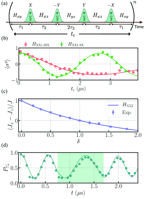
Figure 1: Implementation of XXZ Hamiltonians with two atoms. (a) Microwave sequence consisting of four $\pi/2$-Gaussian pulses driving rotations around $X,-Y,Y,-X$. (b) Evolution of the $y$-magnetization under $H_{\rm driven}$ after initialization in $\ket{\rightarrow\rightarrow}_{y}$ as a function of $t_{c}$, for two ratios $\tau_{1}/\tau_{2}$ corresponding to $\delta=1.33,1.8$. The lines are fit to the data. (c) Normalized oscillation frequency of the $y$-magnetization as a function of $\delta$. Circles: experimental results (error bars from the fits of the oscillations). Solid line: prediction from Eq. (4) with no adjustable parameters. (d) Evolution of the probability $P_{\uparrow\downarrow}$ under $H_{\rm XX}$ and $H_{\rm XXX}$ (green shaded region), following the preparation in $\ket{\uparrow\downarrow}$. Solid lines: simulation using the XXZ Hamiltonian. (b,d) Error bars represent the s.e.m., often smaller than the symbol size.

In this section, we demonstrate the implementation of the XXZ Hamiltonian of Eq. (4) in the case of two interacting atoms. We use the pseudo-spin states $\ket{\downarrow}=\ket{90S_{1/2},m_{J}=1/2}$ and $\ket{\uparrow}=\ket{90P_{3/2},m_{J}=3/2}$ separated by $\omega_{\rm MW}/2\pi=5.1\,\text{GHz}$ and coupled by the microwave field with a mean Rabi frequency averaged over the Gaussian pulses $\Omega=2\pi\times 7.2\,\text{MHz}$. The atoms are separated by $30\,\mu\text{m}$, leading to $J\simeq 2\pi\times 930\,\text{kHz}$.

The spectrum of the XXZ Hamiltonian for two atoms consists of two degenerate eigenstates $\ket{\downarrow\downarrow}$ and $\ket{\uparrow\uparrow}$ with energy $J_{z}$ and two other eigenstates $\ket{\pm}=(\ket{\uparrow\downarrow}\pm\ket{\downarrow\uparrow})/\sqrt{2}$ with energy $-J_{z}\pm 2J_{x}$. To characterize the engineering of the XXZ Hamiltonian, we first initialize the atoms in the state $\ket{\rightarrow\rightarrow}_{y}=(\ket{\uparrow\uparrow}-\ket{\downarrow\downarrow}+i\sqrt{2}\ket{+})/2$, by applying a $\pi/2$ pulse around the $x$-axis. We then apply one sequence of four microwave pulses, varying $t_{c}$ for a fixed ratio $\tau_{1}/\tau_{2}$, i.e., a given anisotropy $\delta$. This state evolves with time, and the total $y$-magnetization $\langle\sigma^{y}\rangle$ oscillates at a frequency $2|J_{x}-J_{z}|$ (see Fig. 1b). We measure this frequency as a function of $\delta$ (see Fig. 1c) and find excellent agreement with the predicted value (Eq. 4).

To demonstrate the dynamical tunability of this microwave engineering, we perform an experiment in which we change the Hamiltonian during the evolution of the system. We initialize the atoms in $\ket{\uparrow\downarrow}$ and measure the probability $P_{\uparrow\downarrow}$ as a function of time. We first let the system evolve under $H_{\rm XX}$ and observe an oscillation between $\ket{\uparrow\downarrow}$ and $\ket{\downarrow\uparrow}$ at a frequency $2J$, see Fig. 1(d). Between $t=0.8-1.7\leavevmode\nobreak\ \mu$s, we apply a single microwave sequence, varying $t_{c}$ while keeping $\tau_{1}=\tau_{2}$ to engineer $H_{\rm XXX}$. We observe a reduction of the oscillation frequency by a factor $0.65(2)$, in agreement with the expected factor of $2/3$. We then switch off the microwaves, and the exchange at frequency $2J$ resumes. This engineering does not introduce extra sizable decoherence beyond the freely evolving case. We compare the results of the experiment with the solution of the Schrödinger equation using the Hamiltonian (Eq. 4). We include the residual imperfections measured on the experiment: SPAM and shot-to-shot fluctuations of the interatomic distance. The results of the simulations are shown as solid lines in Fig. 1(d), and agree well with the data.

V Freezing of the magnetization in a 2D array

We now implement the Hamiltonian engineering technique in a two-dimensional square array consisting of 32 atoms (see Fig. 2). For this purpose, as was done in Ref. [55] for a gas of cold atoms, we engineer the XXX Heisenberg model for which the total magnetization is a conserved quantity. The ability to freeze the magnetization of a system for a controllable time provides a potential route towards dynamical decoupling and quantum sensing [63].

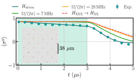
Figure 2: Freezing of the magnetization in a 2D square array. Evolution of the total magnetization along $y$, $\langle\sigma^{y}\rangle$ after initialization in $\ket{\rightarrow\rightarrow\cdots\rightarrow}_{y}$, and evolution under $H_{\rm driven}$ for the first 3 $\mu$s and $H_{\rm XX}$ afterwards. Lines: numerical simulations based on the MACE method (see text). All include SPAM errors. Blue: $H_{\rm driven}$ including the microwave imperfections. Green: without microwave imperfections. Orange: pulse Rabi frequency $\Omega=2\pi\times 28$ MHz, no microwave imperfection. Dashed red: evolution under $H_{\rm XXX}$, followed by $H_{\rm XX}$. Inset: fluorescence image of the 2D square array containing 32 atoms with an inter-site distance $a\simeq 27\,\mu\text{m}$, leading to a nearest-neighbor interaction energy without microwaves $J\simeq 2\pi\times 133\,\text{kHz}$ and a mean interaction energy $J_{m}\simeq 2\pi\times 720\leavevmode\nobreak\$kHz.

For this experiment and for those in the next section, we use the Rydberg states $\ket{\downarrow}=\ket{75S_{1/2},m_{J}=1/2}$ and $\ket{\uparrow}=\ket{75P_{3/2},m_{J}=-1/2}$, separated by $\omega_{\rm MW}/2\pi=8.5$ GHz. We initialize the system in the $\ket{\rightarrow\rightarrow\cdots\rightarrow}_{y}$ state. We apply several sequences of the driven Hamiltonian for $3\,\mu\text{s}$ and then we switch off the drive and let the system evolve under $H_{\rm XX}$. We use $t_{c}=300\,\text{ns}$ and Gaussian microwave pulses with a $1/e^{2}$ width of $16.8$ ns. We measure the total magnetization $\langle\sigma^{y}\rangle$ after the application of an increasing number of sequences. The results are shown in Fig. 2 where, as expected, we observe an approximately constant magnetization for the first $3\,\mu\text{s}$, followed by its decay towards zero under $H_{\rm XX}$. This demagnetization results from the beating of all the eigenfrequencies of $H_{\rm XX}$ for this many-atom system.

As the ab-initio calculation of the dynamics is now more challenging, we use a Moving-Average-Cluster-Expansion (MACE) method [64] to simulate the system. This method consists in diagonalizing clusters, here of 12 atoms, using the Schrödinger equation and averaging the results over all 12-atom cluster configurations possible with 32 atoms. We include in the simulation the SPAM errors and imperfections in the microwave pulses calibrated on a single atom (see Appendix A). As shown in Fig. 2, the simulation, without adjustable parameters, is in good agreement with the observed dynamics at all times. However, the comparison with the evolution under $H_{\rm XXZ}$ (red dashed line) reveals that our engineering is not perfect.

The simulation allows us to assess the contribution of various effects to explain this difference. First, not taking into account the imperfections of the microwave in the simulation (green solid line) leads to a nearly perfect freezing of the magnetization during the application of the pulses: the observed residual decay of the magnetization is thus a consequence of the microwave imperfections. Second, after switching off the microwave field, the dynamics under $H_{\rm XX}$ differs depending on whether it starts from the state produced by $H_{\rm XXX}$ or $H_{\rm driven}$ at $t=3$ $\mu$s. This difference originates from the finite duration of the microwave pulses during which the interactions play a role: an average Rabi frequency four times larger than in the experiment ($\Omega=2\pi\times 28$ MHz, orange curve), would already lead to a nearly perfect agreement between the evolution under $H_{\rm XXX}$ and $H_{\rm driven}$. The agreement finally indicates that the value $J_{m}t_{c}\approx 2\pi\times 0.2$ is already low enough for a faithful implementation of the XXX model.

VI Dynamics of domain wall states in 1D systems

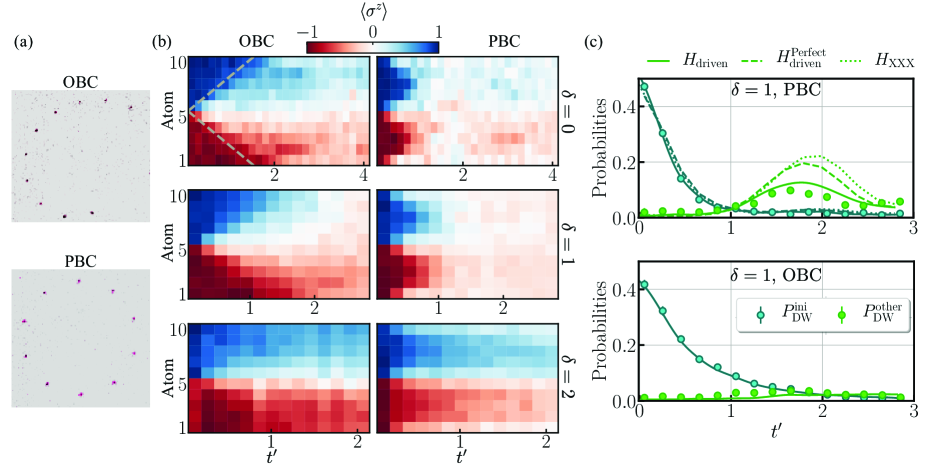
Figure 3: Dynamics of domain wall states under $H_{\rm XXZ}$ in 1D systems. (a) Fluorescence images of the trapped atoms for the two geometries used in the experiment: the spiral implements open boundary conditions (OBC), while the circle realizes periodic boundary conditions (PBC). (b) Density maps of the temporal evolution of the $z$-magnetization $\langle\sigma_{i}^{z}\rangle$ as a function of the normalized time $t^{\prime}$, following the preparation of a domain wall state, for anisotropies $\delta=0,1,2$, and OBC (left) and PBC (right) geometries. The dashed grey line shows the light-cone $\xi=\pm 2Jt^{\prime}$. (c) Evolution of the probability of occurence of domain walls for OBC and PBC. The solid lines are the simulations using $H_{\rm driven}$ accounting for all experimental imperfections (SPAM errors, shot-to-shot fluctuations in atomic positions and microwave imperfections). The dashed (dotted) line is a simulation using $H_{\rm driven}^{\rm Perfect}$ ($H_{\rm XXZ}$) without microwave imperfections.

In a last set of experiments, we illustrate the engineering of $H_{\rm XXZ}$ Hamiltonians on the dynamics of a domain wall (DW), i.e., a situation where a boundary separates spin-up atoms from spin-down ones, in a one-dimensional chain with periodic (PBC) or open (OBC) boundary conditions. Transport properties in the nearest-neighbor XXZ model and for large system sizes have been studied extensively, both analytically and numerically. The evolution of such a system depends on $\delta$ due to two competing effects: a melting of the DW caused by spin-flips with a rate $J_{x}$, and an opposing associated energy cost of $2J_{z}$, which maintains the DW. In the case of a pure initial state (the relevant situation for our experiment), for $\delta<1$, the domain-wall is predicted to melt, with a magnetization profile expanding ballistically in time [65, 66]. At the isotropic point ($\delta=1$), one expects a diffusive behavior with logarithmic corrections [67]. For $\delta>1$, the magnetization profile should be frozen at long times [42, 68, 66]. All these theoretical predictions have been explored for large system sizes.

Here, we study the emergence of these properties with a few-body system of 10 atoms with interatomic distance $a=19\,\mu\text{m}$ (see Fig. 3a). This yields a nearest-neighbor interaction $J\simeq 2\pi\times 270\,\text{kHz}$ and $J_{m}\simeq 2\pi\times 0.6\leavevmode\nobreak\$MHz, which fulfills the condition $J_{m}t_{c}\ll 2\pi$ for $t_{c}=300$ ns. Using the addressing technique described in Sec.III, we prepare five adjacent atoms in $\ket{\uparrow}$ and the remaining ones in $\ket{\downarrow}$. We then study the evolution of the system under $H_{\rm XXZ}$ for different $\delta$.

We first look at the evolution of the single-site magnetization $\langle\sigma_{i}^{z}\rangle$ as a function of the normalized time $t^{\prime}=t\,J_{x}(\delta)/(J\times 1\mu\rm{s})$. The results for OBC are shown in Fig.3(b) with $\delta=0,1,2$ . For $\delta\leq 1$, we observe the melting of the domain wall, resulting in an approximately uniform magnetization profile for $t^{\prime}\gtrsim 3$. In the case $\delta=0$, the width $2\xi$ of the magnetization profile grows ballistically in time, as predicted, and follows a light-cone dynamics, $\xi=\pm 2J\,t^{\prime}$ [65, 66], illustrated by the dashed grey lines in the top left panel of Fig. 3(b). At the isotropic point $\delta=1$, the melting of the wall happens more slowly, as the cost of breaking the spin domains becomes higher. For $\delta=2$, we observe a retention of the domain wall at all times: the magnetization profile hardly evolves between $t^{\prime}=1.1$ and $t^{\prime}=2.0$, indicating a freezing of the system dynamics. Our Hamiltonian engineering is thus able to distinguish different spin-transport behaviors for various $\delta$.

We now consider the case where the atoms are arranged in a circle (PBC). One expects comparable behavior as for the OBC case, with the two domain walls melting ballistically for $\delta=0$, and more slowly for increasing $\delta$. This is what we observe in Fig. 3(b) with the system reaching a depolarized state more quickly than for the OBC due to the presence of two edges. However, the dynamics for $t^{\prime}\gtrsim 1$ differs between PBC and OBC when considering as an observable the probability $P_{\rm DW}$ to observe a given domain wall, as we now illustrate for the case $\delta=1$. The probability $P_{\rm DW}$ is defined as the probability to find a cluster of adjacent $\ket{\uparrow}$ excitations in the chain after an evolution time. The results for the two boundary conditions are shown in Fig. 3(c) where we plot the probability $P_{\rm DW}^{\rm ini}$ to find the initial domain wall after an evolution time $t^{\prime}$ . We do observe the melting of the initial wall, and the fact that it disappears faster for PBC than for OBC. We also plot the probability $P_{\rm DW}^{\rm other}$ to find a domain wall at a location different from the initial one. Interestingly, for PBC, while the average magnetization has reached equilibrium (Fig. 3b) and the initial wall has melted, $P_{\rm DW}^{\rm other}$ still evolves: domain walls appear at different locations around the circle for $t^{\prime}\approx 1.7$ (see also simulations for longer times in App. B). The OBC case shows a much weaker transfer of the initial domain wall towards other ones, thus revealing the role of the boundary conditions (see Fig. A2).

To further understand the domain wall structure around the circle (PBC), we consider the spin correlations $\langle\sigma_{i}^{z}\sigma_{i+1}^{z}\rangle$, related to the number of spin-flips $N_{\text{flip}}$ by:

$$N_{\text{flip}}={1\over 2}\sum_{i}1-\langle\sigma_{i}^{z}\sigma_{i+1}^{z}\rangle$$ (5)

(a flip is defined as two neighboring atoms in opposite spin states). The initialized DW state would therefore consist of two spin flips, while a fully uncorrelated state contains $N/2$ on average. We show in Fig. 4 the dynamics of $N_{\text{flip}}$ for four values of the anisotropy for PBC. For $\delta<1$, $N_{\rm flip}$ approaches $N/2$ at long time, confirming the fact that the system becomes fully uncorrelated. However, for increasing $\delta$, the value of $N_{\rm flip}$ at long times decreases. This means that the $\ket{\uparrow}$ excitations tend to remain bunched for large $\delta$.

We finally compare the experimental data shown in Figs. 3(c) and 4 with numerical simulations using both $H_{\rm driven}$ and the target $H_{\rm XXZ}$ Hamiltonian. For both we include SPAM errors, which are chosen to match the initial state, the residual shot-to-shot fluctuations of the interatomic distances, and the microwave imperfections for $H_{\rm driven}$. The results for the simulation of the probability of domain wall are shown in Fig. 3(c): the data are well approximated by the $H_{\rm driven}$ simulation, indicating that we understand the sources of experimental errors. However, not including the microwave pulses imperfections in the simulation ($H_{\rm driven}^{\rm Perfect}$ in Fig. 3c) reveals a difference with the dynamics driven by $H_{\rm XXZ}$. We show in the Appendix B that this originates from the finite duration of the pulses during which the interaction play a role, as observed in Sec.V. We also plot in Fig. 4 the simulation of $N_{\rm flip}$ using $H_{\rm driven}$, including all the imperfections and find good agreement with the data.

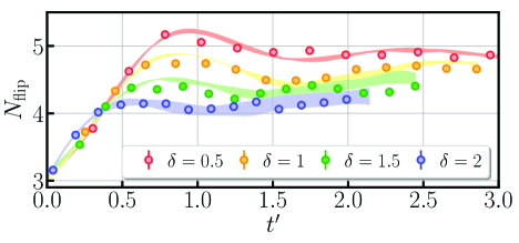
Figure 4: Dynamics of the number of spin flips (PBC). Evolution of $N_{\rm flip}$ for $\delta=0.5,1,1.5,2$ as a function of the normalized time $t^{\prime}$. Shaded regions: results of the simulation using $H_{\rm driven}$, including the $6\pm 1\%$ fluctuations on the microwave rotation axis (see Appendix A).

VII Conclusion

In this work, we have engineered XXZ Hamiltonians with anisotropies $0\leq\delta\leq 2$ using the resonant dipole-dipole interaction between Rydberg atoms in arrays coupled to a resonant microwave field. We have illustrated the method on two iconic situations: the Heisenberg model in 2D square arrays, where we demonstrate the ability to dynamically freeze the evolution of a state with a given magnetization, and the dynamics of a domain wall in a 1D chain with open and periodic boundary conditions. By comparing our results to numerical simulations we infer the two current limitations on our setup: (i) the imperfections in the 8.5 GHz microwave pulses, and (ii) the lack of microwave power that prevents us from reaching pulses short enough to be able to neglect the residual influence of the interactions during their application. Despite these limitations, which can be solved by improving the microwave hardware, we were able to observe all the qualitative features of the situations we explored. This highlights the versatility of a Rydberg-based quantum simulator, beyond the implementation of the natural Ising-like or XX Hamiltonians. Future work could include the study of frustration in various arrays governed by the Heisenberg model [71], or the study of domain wall dynamics for larger system size to confirm the various delocalization scalings beyond the emergent behaviors studied here. We also anticipate that combining microwave drive with the ability to locally address the resonance frequency of the atoms using light-shifts would lead to the engineering of a broader class of Hamiltonians.

Appendix A Calibration of the microwave pulse sequence on a single atom

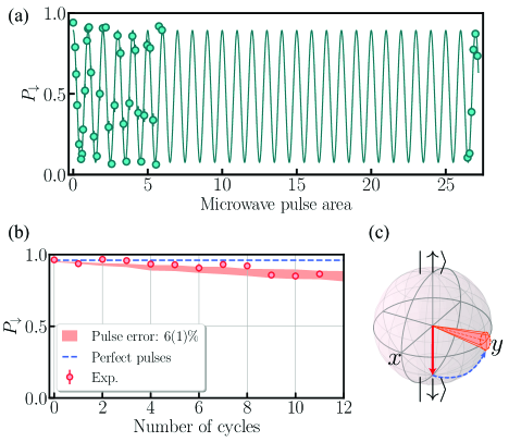
Figure A1: Calibration of microwave pulse error. (a) Microwave Rabi oscillations between states $\ket{\uparrow}$ and $\ket{\downarrow}$. The Rabi frequency is $\Omega=2\pi\times 13.2$ MHz. (b) Probability $P_{\downarrow}$ of measuring a single atom in $\ket{\downarrow}$ following $H_{\rm XXX}$ versus the number of cycles. The data is shown as red circles, with the simulated pulse sequence results for perfect pulses shown in blue and with a pulse error $\Delta\theta=0.06\pm 0.01$ as the shaded pink region. (c) Illustration of how the error is included in the simulation: the final Bloch vector after a rotation around any axis (here the $x$-axis) lies inside the orange cone.

The microwave field is sent onto the atoms using a microwave antenna, with poor control over the polarization due to the presence of metallic parts surrounding the atoms. An example of Rabi oscillation on the $\ket{\downarrow}-\ket{\uparrow}$ transition using a long microwave pulse is shown in Fig. A1(a). We observe no appreciable damping after 25 oscillations.

To implement $H_{\rm driven}$, we have empirically found that applying pulses with Gaussian, rather than square envelopes minimises pulse errors arising from the fast switch on/off. In order to assess the influence of further imperfections in the microwave pulses on the dynamics of the systems used in this work, we compare single atom data with a numerical simulation. We prepare an atom in $\ket{\downarrow}=\ket{75S_{1/2},m_{J}=1/2}$ and then implement sequences of four $\pi/2$- Gaussian pulses, in the same way as for the many-body system. Following a single, four-pulse cycle one would expect the atom to have returned to $\ket{\downarrow}$. Figure A1(b) shows the probability of measuring the atom in $\ket{\downarrow}$ after each cycle, where we see a slow decrease in $P_{\downarrow}$.

In the main text, we concluded that part of the discrepancy between the experimental results and the prediction of the XXZ Hamiltonian simulation came from errors in the microwave pulses. The source of these errors could be fluctuations in the amplitude and/or the phase of the microwave pulses, difficult to measure at frequencies in the 5-10 GHz range. To encompass these effects, we phenomenologically include in our simulations an uncertainty in the angle of rotation of the microwave pulse: for each pulse, we assign two values $n_{1}$ and $n_{2}$ from a normal distribution centered around zero with a standard deviation $\Delta\theta$. We then use these values to describe the rotation operator: if the desired rotation axis is $x$, the actual rotation is performed around the axis $x^{\prime}$ such that

$$\sigma^{x^{\prime}}=(1-n_{1}^{2}-n_{2}^{2})^{1/2}\sigma^{x}+n_{1}\sigma^{y}+n_{2}\sigma^{z}.$$ (A1)

This effect is illustrated in Fig. A1(c). In Fig. A1(b) the shaded area shows an uncertainty in pulse error of $\Delta\theta=0.06\pm 0.01$, which closely matches the experimental results. We use this value of the uncertainty in all the many-body simulations using $H_{\rm driven}$ presented in this work.

Appendix B Influence of the finite duration of the microwave pulses on the simulated many-body Hamiltonian

We have seen in Sec.V that, in the case of the 2D array, increasing the Rabi frequency of the microwave pulses by a factor four, i.e., decreasing their duration by four, leads to a nearly perfect agreement between the evolution under $H_{\rm driven}$ and $H_{\rm XXX}$. We perform here the same analysis for the evolution of the domain wall for both the periodic and open boundary conditions (Sec.VI). The results of the simulation of the probability of domain wall without experimental imperfections is shown in Fig. A2 for an evolution longer than the one achieved in the experiment and for two Rabi frequencies. Similarly to the 2D case, a Rabi frequency four times larger than the one we could reach in the experiment would lead to a very good agreement with the evolution under $H_{\rm XXX}$. This simulation indicates here also that the value $J_{m}t_{c}\approx 2\pi\times 0.2$ is low enough and that the use of discrete pulses does not thwart a faithful implementation of the XXZ Hamiltonian.

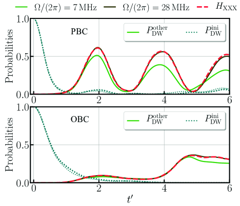
Figure A2: Influence of the finite duration of the microwave pulses. Comparison between the evolution of the probabilities of domain walls under $H_{\rm driven}$ and $H_{\rm XXX}$ in PBC (upper) and OBC (lower). The simulations do not include any experimental error to highlight the role of the finite duration of the microwave pulses, with average Rabi frequency $\Omega$. The large increase of $P_{\rm DW}$ observed for $t^{\prime}>4$ in OBC is a consequence of the reflexion of the excitations at the edges of the chain.

References

- Georgescu et al. [2014] I. M. Georgescu, S. Ashhab, and F. Nori, Quantum simulation, Rev. Mod. Phys. 86, 153 (2014).
- Blatt and Roos [2012] R. Blatt and C. F. Roos, Quantum simulations with trapped ions, Nature Physics 8, 277 (2012).
- Monroe et al. [2021] C. Monroe, W. C. Campbell, L.-M. Duan, Z.-X. Gong, A. V. Gorshkov, P. W. Hess, R. Islam, K. Kim, N. M. Linke, G. Pagano, P. Richerme, C. Senko, and N. Y. Yao, Programmable quantum simulations of spin systems with trapped ions, Rev. Mod. Phys. 93, 025001 (2021).
- Zhou et al. [2011] Y. L. Zhou, M. Ortner, and P. Rabl, Long-range and frustrated spin-spin interactions in crystals of cold polar molecules, Phys. Rev. A 84, 052332 (2011).
- Yan et al. [2013] B. Yan, S. A. Moses, B. Gadway, J. P. Covey, K. R. A. Hazzard, A. M. Rey, D. S. Jin, and J. Ye, Observation of dipolar spin-exchange interactions with lattice-confined polar molecules, Nature 501, 521 (2013).
- Bloch et al. [2012] I. Bloch, J. Dalibard, and S. Nascimbène, Quantum simulations with ultracold quantum gases, Nature Physics 8, 267 (2012).
- Gross and Bloch [2017] C. Gross and I. Bloch, Quantum simulations with ultracold atoms in optical lattices, Science 357, 995 (2017).
- Houck et al. [2012] A. A. Houck, H. E. Türeci, and J. Koch, On-chip quantum simulation with superconducting circuits, Nature Physics 8, 292 (2012).
- Kjaergaard et al. [2020] M. Kjaergaard, M. E. Schwartz, J. Braumüller, P. Krantz, J. I.-J. Wang, S. Gustavsson, and W. D. Oliver, Superconducting qubits: Current state of play, Annual Review of Condensed Matter Physics 11, 369 (2020).
- Goldman and Dalibard [2014] N. Goldman and J. Dalibard, Periodically driven quantum systems: Effective Hamiltonians and engineered gauge fields, Phys. Rev. X 4, 031027 (2014).
- Shirley [1965] J. H. Shirley, Solution of the Schrödinger equation with a Hamiltonian periodic in time, Phys. Rev. 138, B979 (1965).
- Vandersypen and Chuang [2005] L. M. K. Vandersypen and I. L. Chuang, NMR techniques for quantum control and computation, Rev. Mod. Phys. 76, 1037 (2005).
- Salathé et al. [2015] Y. Salathé, M. Mondal, M. Oppliger, J. Heinsoo, P. Kurpiers, A. Potočnik, A. Mezzacapo, U. Las Heras, L. Lamata, E. Solano, S. Filipp, and A. Wallraff, Digital quantum simulation of spin models with circuit quantum electrodynamics, Phys. Rev. X 5, 021027 (2015).
- Jurcevic et al. [2017] P. Jurcevic, H. Shen, P. Hauke, C. Maier, T. Brydges, C. Hempel, B. P. Lanyon, M. Heyl, R. Blatt, and C. F. Roos, Direct observation of dynamical quantum phase transitions in an interacting many-body system, Phys. Rev. Lett. 119, 080501 (2017).
- Peng et al. [2021] P. Peng, C. Yin, X. Huang, C. Ramanathan, and P. Cappellaro, Floquet prethermalization in dipolar spin chains, Nature Physics 17, 444 (2021).
- Rubio-Abadal et al. [2020] A. Rubio-Abadal, M. Ippoliti, S. Hollerith, D. Wei, J. Rui, S. L. Sondhi, V. Khemani, C. Gross, and I. Bloch, Floquet prethermalization in a Bose-Hubbard system, Phys. Rev. X 10, 021044 (2020).
- Kyprianidis et al. [2021] A. Kyprianidis, F. Machado, W. Morong, P. Becker, K. S. Collins, D. V. Else, L. Feng, P. W. Hess, C. Nayak, G. Pagano, N. Y. Yao, and C. Monroe, Observation of a prethermal discrete time crystal, Science 372, 1192 (2021).
- Aidelsburger et al. [2013] M. Aidelsburger, M. Atala, M. Lohse, J. T. Barreiro, B. Paredes, and I. Bloch, Realization of the Hofstadter Hamiltonian with ultracold atoms in optical lattices, Phys. Rev. Lett. 111, 185301 (2013).
- Fläschner et al. [2016] N. Fläschner, B. S. Rem, M. Tarnowski, D. Vogel, D.-S. Lühmann, K. Sengstock, and C. Weitenberg, Experimental reconstruction of the Berry curvature in a Floquet Bloch band, Science 352, 1091 (2016).
- Meinert et al. [2016] F. Meinert, M. J. Mark, K. Lauber, A. J. Daley, and H.-C. Nägerl, Floquet engineering of correlated tunneling in the Bose-Hubbard model with ultracold atoms, Phys. Rev. Lett. 116, 205301 (2016).
- Schweizer et al. [2019] C. Schweizer, F. Grusdt, M. Berngruber, L. Barbiero, E. Demler, N. Goldman, I. Bloch, and M. Aidelsburger, Floquet approach to lattice gauge theories with ultracold atoms in optical lattices, Nature Physics 15, 1168 (2019).
- Eckardt [2017] A. Eckardt, Colloquium: Atomic quantum gases in periodically driven optical lattices, Rev. Mod. Phys. 89, 011004 (2017).
- Wintersperger et al. [2020] K. Wintersperger, C. Braun, F. N. Ünal, A. Eckardt, M. D. Liberto, N. Goldman, I. Bloch, and M. Aidelsburger, Realization of an anomalous Floquet topological system with ultracold atoms, Nature Physics 16, 1058 (2020).
- Browaeys and Lahaye [2020] A. Browaeys and T. Lahaye, Many-body physics with individually controlled Rydberg atoms, Nature Physics 16, 132 (2020).
- Henriet et al. [2020] L. Henriet, L. Beguin, A. Signoles, T. Lahaye, A. Browaeys, G.-O. Reymond, and C. Jurczak, Quantum computing with neutral atoms, Quantum 4, 327 (2020).
- Morgado and Whitlock [2021] M. Morgado and S. Whitlock, Quantum simulation and computing with Rydberg-interacting qubits, AVS Quantum Science 3, 023501 (2021).
- Guardado-Sanchez et al. [2018] E. Guardado-Sanchez, P. T. Brown, D. Mitra, T. Devakul, D. A. Huse, P. Schauß, and W. S. Bakr, Probing the quench dynamics of antiferromagnetic correlations in a 2D quantum Ising spin system, Phys. Rev. X 8, 021069 (2018).
- Lienhard et al. [2018] V. Lienhard, S. de Léséleuc, D. Barredo, T. Lahaye, A. Browaeys, M. Schuler, L.-P. Henry, and A. M. Läuchli, Observing the space- and time-dependent growth of correlations in dynamically tuned synthetic Ising antiferromagnets, Phys. Rev. X 8, 021070 (2018).
- Scholl et al. [2021] P. Scholl, M. Schuler, H. J. Williams, A. A. Eberharter, D. Barredo, K.-N. Schymik, V. Lienhard, L.-P. Henry, T. C. Lang, T. Lahaye, A. M. Läuchli, and A. Browaeys, Quantum simulation of 2D antiferromagnets with hundreds of Rydberg atoms, Nature 595, 233 (2021).
- Song et al. [2021] Y. Song, M. Kim, H. Hwang, W. Lee, and J. Ahn, Quantum simulation of Cayley-tree Ising Hamiltonians with three-dimensional Rydberg atoms, Phys. Rev. Research 3, 013286 (2021).
- Keesling et al. [2019] A. Keesling, A. Omran, H. Levine, H. Bernien, H. Pichler, S. Choi, R. Samajdar, S. Schwartz, P. Silvi, S. Sachdev, P. Zoller, M. Endres, M. Greiner, V. Vuletic, and M. D. Lukin, Quantum Kibble-Zurek mechanism and critical dynamics on a programmable Rydberg simulator, Nature 568, 207 (2019).
- Ebadi et al. [2021] S. Ebadi, T. T. Wang, H. Levine, A. Keesling, G. Semeghini, A. Omran, D. Bluvstein, R. Samajdar, H. Pichler, W. W. Ho, S. Choi, S. Sachdev, M. Greiner, V. Vuletić, and M. D. Lukin, Quantum phases of matter on a 256-atom programmable quantum simulator, Nature 595, 227 (2021).
- Semeghini et al. [2021] G. Semeghini, H. Levine, A. Keesling, S. Ebadi, T. T. Wang, D. Bluvstein, R. Verresen, H. Pichler, M. Kalinowski, R. Samajdar, A. Omran, S. Sachdev, A. Vishwanath, M. Greiner, V. Vuletić, and M. D. Lukin, Probing topological spin liquids on a programmable quantum simulator, Science 374, 1242 (2021), https://www.science.org/doi/pdf/10.1126/science.abi8794 .
- Lienhard et al. [2020] V. Lienhard, P. Scholl, S. Weber, D. Barredo, S. de Léséleuc, R. Bai, N. Lang, M. Fleischhauer, H. P. Büchler, T. Lahaye, and A. Browaeys, Realization of a density-dependent Peierls phase in a synthetic, spin-orbit coupled Rydberg system, Phys. Rev. X 10, 021031 (2020).
- de Léséleuc et al. [2019] S. de Léséleuc, V. Lienhard, P. Scholl, D. Barredo, S. Weber, N. Lang, H. P. Büchler, T. Lahaye, and A. Browaeys, Observation of a symmetry-protected topological phase of interacting bosons with Rydberg atoms, Science 365, 775 (2019).
- Whitlock et al. [2017] S. Whitlock, A. W. Glaetzle, and P. Hannaford, Simulating quantum spin models using Rydberg-excited atomic ensembles in magnetic microtrap arrays, Journal of Physics B: Atomic, Molecular and Optical Physics 50, 074001 (2017).
- Signoles et al. [2021] A. Signoles, T. Franz, R. Ferracini Alves, M. Gärttner, S. Whitlock, G. Zürn, and M. Weidemüller, Glassy dynamics in a disordered Heisenberg quantum spin system, Phys. Rev. X 11, 011011 (2021).
- Nguyen et al. [2018] T. L. Nguyen, J. M. Raimond, C. Sayrin, R. Cortiñas, T. Cantat-Moltrecht, F. Assemat, I. Dotsenko, S. Gleyzes, S. Haroche, G. Roux, T. Jolicoeur, and M. Brune, Towards quantum simulation with circular Rydberg atoms, Phys. Rev. X 8, 011032 (2018).
- Dmitriev et al. [2002] D. V. Dmitriev, V. Y. Krivnov, A. A. Ovchinnikov, and A. Langari, One-dimensional anisotropic Heisenberg model in the transverse magnetic field, J. Exp. Theor. Phys. 95, 538 (2002).
- Wei et al. [2018] K. X. Wei, C. Ramanathan, and P. Cappellaro, Exploring localization in nuclear spin chains, Phys. Rev. Lett. 120, 070501 (2018).
- Cheneau et al. [2012] M. Cheneau, P. Barmettler, D. Poletti, M. Endres, P. Schauß, T. Fukuhara, C. Gross, I. Bloch, C. Kollath, and S. Kuhr, Light-cone-like spreading of correlations in a quantum many-body system, Nature 481, 484 (2012).
- Gobert et al. [2005] D. Gobert, C. Kollath, U. Schollwöck, and G. Schütz, Real-time dynamics in spin- chains with adaptive time-dependent density matrix renormalization group, Phys. Rev. E 71, 036102 (2005).
- Sirker et al. [2009] J. Sirker, R. G. Pereira, and I. Affleck, Diffusion and ballistic transport in one-dimensional quantum systems, Phys. Rev. Lett. 103, 216602 (2009).
- Barmettler et al. [2009] P. Barmettler, M. Punk, V. Gritsev, E. Demler, and E. Altman, Relaxation of antiferromagnetic order in spin- chains following a quantum quench, Phys. Rev. Lett. 102, 130603 (2009).
- Bertini et al. [2021] B. Bertini, F. Heidrich-Meisner, C. Karrasch, T. Prosen, R. Steinigeweg, and M. Žnidarič, Finite-temperature transport in one-dimensional quantum lattice models, Rev. Mod. Phys. 93, 025003 (2021).
- Giamarchi [2003] T. Giamarchi, Quantum physics in one dimension (Clarendon Press, 2003).
- Jepsen et al. [2020] P. N. Jepsen, J. Amato-Grill, I. Dimitrova, W. W. Ho, E. Demler, and W. Ketterle, Spin transport in a tunable Heisenberg model realized with ultracold atoms, Nature 588, 403 (2020).
- Hild et al. [2014] S. Hild, T. Fukuhara, P. Schauß, J. Zeiher, M. Knap, E. Demler, I. Bloch, and C. Gross, Far-from-equilibrium spin transport in Heisenberg quantum magnets, Phys. Rev. Lett. 113, 147205 (2014).
- Wei et al. [2021] D. Wei, A. Rubio-Abadal, B. Ye, F. Machado, J. Kemp, K. Srakaew, S. Hollerith, J. Rui, S. Gopalakrishnan, N. Y. Yao, I. Bloch, and J. Zeiher, Quantum gas microscopy of Kardar-Parisi-Zhang superdiffusion (2021), arXiv:2107.00038 .
- Joshi et al. [2021] M. K. Joshi, F. Kranzl, A. Schuckert, I. Lovas, C. Maier, R. Blatt, M. Knap, and C. F. Roos, Observing emergent hydrodynamics in a long-range quantum magnet (2021), arXiv:2107.00033 .
- Richerme et al. [2014] P. Richerme, Z.-X. Gong, A. Lee, C. Senko, J. Smith, M. Foss-Feig, S. Michalakis, A. V. Gorshkov, and C. Monroe, Non-local propagation of correlations in quantum systems with long-range interactions, Nature 511, 198 (2014).
- Jurcevic et al. [2014] P. Jurcevic, B. P. Lanyon, P. Hauke, C. Hempel, P. Zoller, R. Blatt, and C. F. Roos, Quasiparticle engineering and entanglement propagation in a quantum many-body system, Nature 511, 202 (2014).
- Tan et al. [2021] W. L. Tan, P. Becker, F. Liu, G. Pagano, K. S. Collins, A. De, L. Feng, H. B. Kaplan, A. Kyprianidis, R. Lundgren, W. Morong, S. Whitsitt, A. V. Gorshkov, and C. Monroe, Domain-wall confinement and dynamics in a quantum simulator, Nature Physics 17, 742 (2021).
- Fukuhara et al. [2013] T. Fukuhara, P. Schauß, M. Endres, S. Hild, M. Cheneau, I. Bloch, and C. Gross, Microscopic observation of magnon bound states and their dynamics, Nature 502, 76 (2013).
- Geier et al. [2021] S. Geier, N. Thaicharoen, C. Hainaut, T. Franz, A. Salzinger, A. Tebben, D. Grimshandl, G. Zürn, and M. Weidemüller, Floquet hamiltonian engineering of an isolated many-body spin system, Science 374, 1149 (2021), https://www.science.org/doi/pdf/10.1126/science.abd9547 .
- Barredo et al. [2018] D. Barredo, V. Lienhard, S. de Léséleuc, T. Lahaye, and A. Browaeys, Synthetic three-dimensional atomic structures assembled atom by atom, Nature 561, 79 (2018).
- Nogrette et al. [2014] F. Nogrette, H. Labuhn, S. Ravets, D. Barredo, L. Béguin, A. Vernier, T. Lahaye, and A. Browaeys, Single-atom trapping in holographic 2D arrays of microtraps with arbitrary geometries, Phys. Rev. X 4, 021034 (2014).
- Schymik et al. [2020] K.-N. Schymik, V. Lienhard, D. Barredo, P. Scholl, H. Williams, A. Browaeys, and T. Lahaye, Enhanced atom-by-atom assembly of arbitrary tweezer arrays, Phys. Rev. A 102, 063107 (2020).
- Note [1] Tabor Electronics Ltd. SE5081.
- de Léséleuc et al. [2017] S. de Léséleuc, D. Barredo, V. Lienhard, A. Browaeys, and T. Lahaye, Optical control of the resonant dipole-dipole interaction between Rydberg atoms, Phys. Rev. Lett. 119, 053202 (2017).
- Note [2] For the experiments beyond two atoms, prior to sending the 1013 nm de-excitation laser, we first apply a microwave pulse of ns to transfer atoms in to , which has a much smaller coupling to . This procedure leads to a freezing of the interaction-induced dynamics.
- de Léséleuc et al. [2018] S. de Léséleuc, D. Barredo, V. Lienhard, A. Browaeys, and T. Lahaye, Analysis of imperfections in the coherent optical excitation of single atoms to Rydberg states, Phys. Rev. A 97, 053803 (2018).
- Choi et al. [2020] J. Choi, H. Zhou, H. S. Knowles, R. Landig, S. Choi, and M. D. Lukin, Robust dynamic Hamiltonian engineering of many-body spin systems, Phys. Rev. X 10, 031002 (2020).
- Hazzard et al. [2014] K. R. A. Hazzard, B. Gadway, M. Foss-Feig, B. Yan, S. A. Moses, J. P. Covey, N. Y. Yao, M. D. Lukin, J. Ye, D. S. Jin, and A. M. Rey, Many-body dynamics of dipolar molecules in an optical lattice, Phys. Rev. Lett. 113, 195302 (2014).
- Collura et al. [2018] M. Collura, A. De Luca, and J. Viti, Analytic solution of the domain-wall nonequilibrium stationary state, Phys. Rev. B 97, 081111 (2018).
- Misguich et al. [2019] G. Misguich, N. Pavloff, and V. Pasquier, Domain wall problem in the quantum XXZ chain and semiclassical behavior close to the isotropic point, SciPost Physics 7, 025 (2019).
- Misguich et al. [2017] G. Misguich, K. Mallick, and P. L. Krapivsky, Dynamics of the spin- Heisenberg chain initialized in a domain-wall state, Phys. Rev. B 96, 195151 (2017).
- Mossel and Caux [2010] J. Mossel and J.-S. Caux, Relaxation dynamics in the gapped XXZ spin- chain, New J. Phys. 12, 055028 (2010).
- Note [3] Implementing requires . We therefore remove the and pulses from the sequence, with the exception of the first and final pulses.
- Note [4] To increase the amplitude of the revival in observed in Fig. 3(c) we include in the data and in the simulations events containing domain walls with 4, 5 and 6 excitations.
- Richter et al. [2004] J. Richter, J. Schulenburg, and A. Honecker, Quantum magnetism in two dimensions: From semi-classical Néel order to magnetic disorder, in Quantum magnetism. Lecture Notes in Physics, edited by U. Schollwöck, J. Richter, D. Farnell, and R. Bishop (Springer, Berlin, 2004) pp. 85–153.