Universal cutoff for Dyson Ornstein Uhlenbeck process

Abstract.

We study the Dyson–Ornstein–Uhlenbeck diffusion process, an evolving gas of interacting particles. Its invariant law is the beta Hermite ensemble of random matrix theory, a non-product log-concave distribution. We explore the convergence to equilibrium of this process for various distances or divergences, including total variation, relative entropy, and transportation cost. When the number of particles is sent to infinity, we show that a cutoff phenomenon occurs: the distance to equilibrium vanishes abruptly at a critical time. A remarkable feature is that this critical time is independent of the parameter beta that controls the strength of the interaction, in particular the result is identical in the non-interacting case, which is nothing but the Ornstein–Uhlenbeck process. We also provide a complete analysis of the non-interacting case that reveals some new phenomena. Our work relies among other ingredients on convexity and functional inequalities, exact solvability, exact Gaussian formulas, coupling arguments, stochastic calculus, variational formulas and contraction properties. This work leads, beyond the specific process that we study, to questions on the high-dimensional analysis of heat kernels of curved diffusions.

1. Introduction and main results

Let us consider a Markov process $X={(X_{t})}_{t\geq 0}$ with state space $S$ and invariant law $\mu$ for which

$$\lim_{t\to\infty}\mathrm{dist}(\mathrm{Law}(X_{t})\mid\mu)=0$$

where $\mathrm{dist}(\cdot\mid\cdot)$ is a distance or divergence on the probability measures on $S$. Suppose now that $X=X^{n}$ depends on a dimension, size, or complexity parameter $n$, and let us set $S=S^{n}$, $\mu=\mu^{n}$, and $X_{0}=x^{n}_{0}\in S^{n}$. For example $X^{n}$ can be a random walk on the symmetric group of permutations of $\{1,\ldots,n\}$, Brownian motion on the group of $n\times n$ unitary matrices, Brownian motion on the $n$-dimensional sphere, etc. In many of such examples, it has been proved that when $n$ is large enough, the supremum over some set of initial conditions $x^{n}_{0}$ of the quantity $\mathrm{dist}(\mathrm{Law}(X_{t}^{n})\mid\mu^{n})$ collapses abruptly to $0$ when $t$ passes a critical value $c=c_{n}$ which may depend on $n$. This is often referred to as a cutoff phenomenon. More precisely, if $\mathrm{dist}$ ranges from $0$ to $\max$, then, for some subset $S^{n}_{0}\subset S^{n}$ of initial conditions, some critical value $c=c_{n}$ and for all $\varepsilon\in(0,1)$,

$$\lim_{n\to\infty}\sup_{x^{n}_{0}\in S^{n}_{0}}\mathrm{dist}(\mathrm{Law}(X^{n}_{t_{n}})\mid\mu^{n})=\begin{cases}\max&\text{if $t_{n}=(1-\varepsilon)c_{n}$}\\ 0&\text{if $t_{n}=(1+\varepsilon)c_{n}$}\end{cases}.$$

It is standard to introduce, for an arbitrary small threshold $\eta>0$, the quantity $\inf\{t\geq 0:\sup_{x_{0}\in S_{0}^{n}}\mathrm{dist}(\mathrm{Law}(X^{n}_{t})\mid\mu^{n})\leq\eta\}$ known as the mixing time in the literature. Of course such a definition fully makes sense as soon as $t\mapsto{\sup_{x_{0}\in S_{0}^{n}}}\mathrm{dist}(\mathrm{Law}(X^{n}_{t})\mid\mu^{n})$ is non-increasing.

When $S^{n}$ is finite, it is customary to take $S^{n}_{0}=S^{n}$. When $S^{n}$ is infinite, it may happen that the supremum over the whole set $S^{n}$ of the distance to equilibrium remains equal to $\max$ at all times, in which case one has to consider strict subspaces of initial conditions. For some processes, it is possible to restrict $S^{n}_{0}$ to a single state in which case one obtains a very precise description of the convergence to equilibrium starting from this initial condition. Note that the constraint over the initial condition can be made compatible with a limiting dynamics, for instance a mean-field limit when the process describes an exchangeable interacting particle system.

The cutoff phenomenon was put forward by Aldous and Diaconis at the origin for random walks on finite sets, see for instance [1, 28, 26, 52] and references therein. The analysis of the cutoff phenomenon is the subject of an important activity, still seeking for a complete theory: let us mention that, for the total variation distance, Peres proposed the so-called product condition (the mixing time must be much larger than the inverse of the spectral gap) as a necessary and sufficient condition for a cutoff phenomenon to hold, but counter-examples were exhibited [52, Sec. 18.3] and the product condition is only necessary.

The study of the cutoff phenomenon for Markov diffusion processes goes back at least to the works of Saloff-Coste [62, 64] in relation notably with Nash–Sobolev type functional inequalities, heat kernel analysis, and Diaconis–Wilson probabilistic techniques. We also refer to the more recent work [55] for the case of diffusion processes on compact groups and symmetric spaces, in relation with group invariance and representation theory, a point of view inspired by the early works of Diaconis on Markov chains and of Saloff-Coste on diffusion processes. Even if most of the available results in the literature on the cutoff phenomenon are related to compact state spaces, there are some notable works devoted to non-compact spaces such as [47, 19, 10, 8, 9, 11].

Our contribution is an exploration of the cutoff phenomenon for the Dyson–Ornstein–Uhlenbeck diffusion process, for which the state space is $\mathbb{R}^{n}$. This process is an interacting particle system. When the interaction is turned off, we recover the Ornstein–Uhlenbeck process, a special case that has been considered previously in the literature but for which we also provide new results.

1.1. Distances

As for $\mathrm{dist}$ we use several standard distances or divergences between probability measures: Wasserstein, total variation (TV), Hellinger, Entropy, $\chi^{2}$ and Fisher, surveyed in Appendix A. We take the following convention for probability measures $\mu$ and $\nu$ on the same space:

$$\mathrm{dist}(\mu\mid\nu)=\begin{cases}\mathrm{Wasserstein}(\mu,\nu)&\text{when $\mathrm{dist}=\mathrm{Wasserstein}$}\\ \left\|\mu-\nu\right\|_{\mathrm{TV}}&\text{when $\mathrm{dist}=\mathrm{TV}$}\\ \mathrm{Hellinger}(\mu,\nu)&\text{when $\mathrm{dist}=\mathrm{Hellinger}$}\\ \mathrm{Kullback}(\mu\mid\nu)&\text{when $\mathrm{dist}=\mathrm{Kullback}$}\\ \chi^{2}(\mu\mid\nu)&\text{when $\mathrm{dist}=\chi^{2}$}\\ \mathrm{Fisher}(\mu\mid\nu)&\text{when $\mathrm{dist}=\mathrm{Fisher}$}\end{cases},$$ (1.1)

see Appendix A for precise definitions. The maximal value $\max$ taken by $\mathrm{dist}$ is given by

$$\max=\begin{cases}1&\text{ if }\mathrm{dist}\in\{\mathrm{TV},\mathrm{Hellinger}\},\\ +\infty&\text{ if }\mathrm{dist}\in\{\mathrm{Wasserstein},\mathrm{Kullback},\chi^{2},\mathrm{Fisher}\}.\end{cases}$$ (1.2)

1.2. The Dyson–Ornstein–Uhlenbeck (DOU) process and preview of main results

The DOU process is the solution $X^{n}={(X^{n}_{t})}_{t\geq 0}$ on $\mathbb{R}^{n}$ of the stochastic differential equation

$$X^{n}_{0}=x^{n}_{0}\in\mathbb{R}^{n},\quad\mathrm{d}X_{t}^{n,i}=\sqrt{\frac{2}{n}}\mathrm{d}B^{i}_{t}-V^{\prime}(X_{t}^{n,i})\mathrm{d}t+\frac{\beta}{n}\sum_{j\neq i}\frac{\mathrm{d}t}{X_{t}^{n,i}-X_{t}^{n,j}},\quad 1\leq i\leq n,$$ (1.3)

where ${(B_{t})}_{t\geq 0}$ is a standard $n$-dimensional Brownian motion (BM), and where

• $V(x)=\frac{x^{2}}{2}$ is a “confinement potential” acting through the drift $-V^{\prime}(x)=-x$

• $\beta\geq 0$ is a parameter tuning the interaction strength.

The notation $X^{n,i}_{t}$ stands for the $i$-th coordinate of the vector $X^{n}_{t}$. The process $X^{n}$ can be thought of as an interacting particle system of $n$ one-dimensional Brownian particles $X^{n,1},\ldots,X^{n,n}$, subject to confinement and singular pairwise repulsion when $\beta>0$ (respectively first and second term in the drift). We take an inverse temperature of order $n$ in (1.3) in order to obtain a mean-field limit without time-changing the process, see Section 2.5. The spectral gap is $1$ for all $n\geq 1$, see Section 2.6. We refer to Section 2.9 for other parametrizations or choices of inverse temperature.

In the special cases $\beta\in\{0,1,2\}$, the cutoff phenomenon for the DOU process can be established by using Gaussian analysis and stochastic calculus, see Sections 1.4 and 1.5. For $\beta=0$, the process reduces to the Ornstein–Uhlenbeck process (OU) and its behavior serves as a benchmark for the interaction case $\beta\neq 0$, while when $\beta\in\{1,2\}$, the approach involves a lift to unitary invariant ensembles of random matrix theory. For a general $\beta\geq 1$, our main results regarding the cutoff phenomenon for the DOU process are given in Sections 1.6 and 1.7. We are able, in particular, to prove the following: for all $\mathrm{dist}\in\{\mathrm{Wasserstein},\mathrm{TV},\mathrm{Hellinger}\}$, $a>0$, $\varepsilon\in(0,1)$, we have

$$\lim_{n\to\infty}\sup_{x^{n}_{0}\in[-a,a]^{n}}\mathrm{dist}(\mathrm{Law}(X^{n}_{t_{n}})\mid P_{n}^{\beta})=\begin{cases}\max&\text{if $t_{n}=(1-\varepsilon)c_{n}$}\\ 0&\text{if $t_{n}=(1+\varepsilon)c_{n}$}\end{cases},$$

where $P_{n}^{\beta}$ is the invariant law of the process, and where

$$c_{n}:=\begin{cases}\log(\sqrt{n}a)&\text{ if $\mathrm{dist}=\mathrm{Wasserstein}$}\\ \log(na)&\text{ if $\mathrm{dist}\in\{\mathrm{TV},\mathrm{Hellinger}\}$}\end{cases}.$$

This result is stated in a slightly more general form in Corollary 1.7. Our proof relies crucially on an exceptional exact solvability of the dynamics, notably the fact that we know explicitly the optimal long time behavior in entropy and coupling distance, as well as the eigenfunction associated to the spectral gap which turns out to be linear and optimal. This comes from the special choice of $V$ as well as the special properties of the Coulomb interaction. We stress that such an exact solvability is no longer available for a general strongly convex $V$, even for instance in the simple example $V(x)=\frac{x^{2}}{2}+x^{4}$ or for general linear forces. Nevertheless, and as usual, two other special classical choices of $V$ could be explored, related to Laguerre and Jacobi weights, see Section 2.8.

1.3. Analysis of the Dyson–Ornstein–Uhlenbeck process

The process $X^{n}$ was essentially discovered by Dyson in [33], in the case $\beta\in\{1,2,4\}$, because it describes the dynamics of the eigenvalues of $n\times n$ symmetric/Hermitian/symplectic random matrices with independent Ornstein–Uhlenbeck entries, see Lemma 5.1 and Lemma 5.2 below for the cases $\beta=1$ and $\beta=2$ respectively.

• Case $\beta=0$ (interaction turned off). The particles become $n$ independent one-dimensional Ornstein–Uhlenbeck processes, and the DOU process $X^{n}$ becomes exactly the $n$-dimensional Ornstein–Uhlenbeck process $Z^{n}$ solving (1.8). The process lives in $\mathbb{R}^{n}$. The particles collide but since they do not interact, this does not raise any issue.

• Case $0<\beta<1$. Then with positive probability the particles collide producing a blow up of the drift, see for instance [22, 25] for a discussion. Nevertheless, it is possible to define the process for all times, for instance by adding a local time term to the stochastic differential equation, see [25] and references therein. It is natural to expect that the cutoff universality works as for $\beta\not\in(0,1)$, but for simplicity we do not consider this case here.

• Case $\beta\geq 1$. If we order the coordinates by defining the convex domain

  $$D_{n}=\{x\in\mathbb{R}^{n}:x_{1}<\cdots<x_{n}\},$$

  and if $x^{n}_{0}\in D_{n}$ then the equation (1.3) admits a unique strong solution that never exits $D_{n}$, in other words the particles never collide and the order of the initial particles is preserved at all times, see [60]. Moreover if

  $$\overline{D}_{n}=\{x\in\mathbb{R}^{n}:x_{1}\leq\cdots\leq x_{n}\}$$

  then it is possible to start the process from the boundary $\overline{D}_{n}\setminus D_{n}$, in particular from $x^{n}_{0}$ such that $x^{n,1}_{0}=\cdots=x^{n,n}_{0}$, and despite the singularity of the drift, it can be shown that with probability one, $X^{n}_{t}\in D_{n}$ for all $t>0$. We refer to [2, Th. 4.3.2] for a proof in the Dyson Brownian Motion case that can be adapted mutatis mutandis.

In the sequel, we will only consider the cases $\beta=0$ with $x_{0}^{n}\in\mathbb{R}^{n}$ and $\beta\geq 1$ with $x^{n}_{0}\in\overline{D}_{n}$.

The drift in (1.3) is the gradient of a function, and (1.3) rewrites

$$X_{0}^{n}=x_{0}^{n}\in D_{n},\quad\mathrm{d}X_{t}^{n}=\sqrt{\frac{2}{n}}\mathrm{d}B_{t}-\frac{1}{n}\nabla E(X_{t}^{n})\mathrm{d}t,$$ (1.4)

where

$$E(x_{1},\ldots,x_{n})=n\sum_{i=1}^{n}V(x_{i})+{\beta}\sum_{i>j}\log\frac{1}{|x_{i}-x_{j}|}$$ (1.5)

can be interpreted as the energy of the configuration of particles $x_{1},\ldots,x_{n}$.

• If $\beta=0$, then the Markov process $X^{n}$ is an Ornstein–Uhlenbeck process, irreducible with unique invariant law $P_{n}^{0}=\mathcal{N}(0,\frac{1}{n}I_{n})$ which is reversible.

• If $\beta\geq 1$, then the Markov process $X^{n}$ is not irreducible, but $D_{n}$ is a recurrent class carrying a unique invariant law $P_{n}^{\beta}$, which is reversible and given by

  $$P_{n}^{\beta}=\frac{\mathrm{e}^{-E(x_{1},\ldots,x_{n})}}{C_{n}^{\beta}}\mathbf{1}_{(x_{1},\ldots,x_{n})\in\overline{D}_{n}}\mathrm{d}x_{1}\cdots\mathrm{d}x_{n},$$ (1.6)

  where $C_{n}^{\beta}$ is the normalizing factor given by

  $$C_{n}^{\beta}=\int_{\overline{D}_{n}}\mathrm{e}^{-E(x_{1},\ldots,x_{n})}\mathrm{d}x_{1}\cdots\mathrm{d}x_{n}.$$ (1.7)

In terms of geometry, it is crucial to observe that since $-\log$ is convex on $(0,+\infty)$, the map

$$(x_{1},\ldots,x_{n})\in D_{n}\mapsto\mathrm{Interaction}(x_{1},\ldots,x_{n})={\beta}\sum_{i>j}\log\frac{1}{x_{i}-x_{j}},$$

is convex. Thus, since $V$ is convex on $\mathbb{R}$, it follows that $E$ is convex on $D_{n}$. For all $\beta\geq 0$, the law $P_{n}^{\beta}$ is log-concave with respect to the Lebesgue measure as well as with respect to $\mathcal{N}(0,\frac{1}{n}I_{n})$.

1.4. Non-interacting case and Ornstein–Uhlenbeck benchmark

When we turn off the interaction by taking $\beta=0$ in (1.3), the DOU process becomes an Ornstein–Uhlenbeck process (OU) $Z^{n}={(Z^{n}_{t})}_{t\geq 0}$ on $\mathbb{R}^{n}$ solving the stochastic differential equation

$$Z^{n}_{0}=z^{n}_{0}\in\mathbb{R}^{n},\quad\mathrm{d}Z^{n}_{t}=\sqrt{\frac{2}{n}}\mathrm{d}B^{n}_{t}-Z^{n}_{t}\mathrm{d}t,$$ (1.8)

where $B^{n}$ is a standard $n$-dimensional BM. The invariant law of $Z^{n}$ is the product Gaussian law $P_{n}^{0}=\mathcal{N}(0,\frac{1}{n}I_{n})=\mathcal{N}(0,\frac{1}{n})^{\otimes n}$. The explicit Gaussian nature of $Z_{t}^{n}\sim\mathcal{N}(z_{0}^{n}\mathrm{e}^{-t},\frac{1-\mathrm{e}^{-2t}}{n}I_{n})$, valid for all $t\geq 0$, allows for a fine analysis of convergence to equilibrium, as in the following theorem.

Theorem 1.1 (Cutoff for OU: mean-field regime).

Let $Z^{n}={(Z^{n}_{t})}_{t\geq 0}$ be the OU process (1.8) and let $P_{n}^{0}$ be its invariant law. Suppose that

$$\varliminf_{n\to\infty}\frac{|z^{n}_{0}|^{2}}{n}>0\quad\text{and}\quad\varlimsup_{n\to\infty}\frac{|z^{n}_{0}|^{2}}{n}<\infty$$

where $|z|=\sqrt{z_{1}^{2}+\cdots+z_{n}^{2}}$ is the Euclidean norm. Then for all $\varepsilon\in(0,1)$,

$$\lim_{n\to\infty}\mathrm{dist}(\mathrm{Law}(Z^{n}_{t_{n}})\mid P_{n}^{0})=\begin{cases}\max&\text{if $t_{n}=(1-\varepsilon)c_{n}$}\\ 0&\text{if $t_{n}=(1+\varepsilon)c_{n}$}\end{cases}$$

where

$$c_{n}=\begin{cases}\frac{1}{2}\log(n)&\text{if $\mathrm{dist}=\mathrm{Wasserstein}$},\\ \log(n)&\text{if $\mathrm{dist}\in\{\mathrm{TV},\mathrm{Hellinger},\mathrm{Kullback},\chi^{2}\}$},\\ \frac{3}{2}\log(n)&\text{if $\mathrm{dist}=\mathrm{Fisher}$}.\end{cases}$$

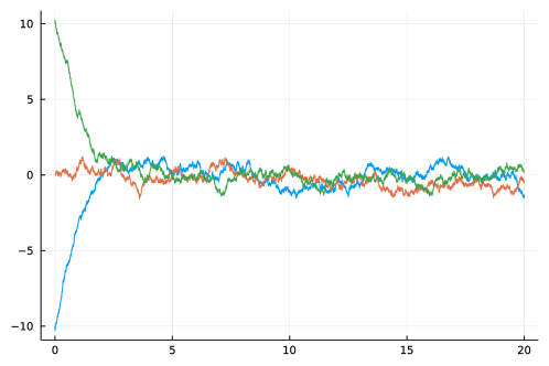
Figure 1. A trajectory of a single DOU with $n=3$ and $x^{n}_{0}=(-10,0,10)$, $\beta=0$ on top and $\beta=2$ on bottom. The driving Brownian motions are the same.

Theorem 1.1 is proved in Section 3. See Figure 1 and Figure 2 for a numerical experiment.

Theorem 1.1 constitutes a very natural benchmark for the cutoff phenomenon for the DOU process. Theorem 1.1 is not a surprise, and actually the TV and Hellinger cases are already considered in [47], see also [7]. Let us mention that in [9], a cutoff phenomenon for TV, entropy and Wasserstein is proven for the OU process of fixed dimension $d$ and vanishing noise. This is to be compared with our setting where the dimension is sent to infinity: the results (and their proofs) are essentially the same in these two situations, however we will see below that if one considers more general initial conditions, there are some substantial differences according to whether the dimension is fixed or sent to infinity.

The restriction over the initial condition in Theorem 1.1 is spelled out in terms of the second moment of the empirical distribution, a natural choice suggested by the mean-field limit discussed in Section 2.5. It yields a mixing time of order $\log(n)$, just like for Brownian motion on compact Lie groups, see [64, 55]. For the OU process and more generally for overdamped Langevin processes, the non-compactness of the space is replaced by the confinement or tightness due to the drift.

Actually, Theorem 1.1 is a particular instance of the following, much more general result that reveals that, except for the Wasserstein distance, a cutoff phenomenon always occurs.

Theorem 1.2 (General cutoff for OU).

Let $Z^{n}={(Z^{n}_{t})}_{t\geq 0}$ be the OU process (1.8) and let $P_{n}^{0}$ be its invariant law. Let $\mathrm{dist}\in\{\mathrm{TV},\mathrm{Hellinger},\mathrm{Kullback},\chi^{2},\mathrm{Fisher}\}$. Then, for all $\varepsilon\in(0,1)$,

$$\lim_{n\to\infty}\mathrm{dist}(\mathrm{Law}(Z^{n}_{t_{n}})\mid P_{n}^{0})=\begin{cases}\max&\text{if $t_{n}=(1-\varepsilon)c_{n}$,}\\ 0&\text{if $t_{n}=(1+\varepsilon)c_{n}$}\end{cases}$$

where

$$c_{n}=\begin{cases}\log(\sqrt{n}|z_{0}^{n}|)\vee\frac{1}{4}\log(n)&\text{if $\mathrm{dist}\in\{\mathrm{TV},\mathrm{Hellinger},\mathrm{Kullback},\chi^{2}\}$},\\ \log(n|z_{0}^{n}|)\vee\frac{1}{2}\log(n)&\text{if $\mathrm{dist}=\mathrm{Fisher}$}.\end{cases}$$

Regarding the Wasserstein distance, the following dichotomy occurs:

• if $\lim_{n\to\infty}|z_{0}^{n}|=+\infty$, then for all $\varepsilon\in(0,1)$, with $c_{n}=\log|z_{0}^{n}|$,

  $$\lim_{n\to\infty}\mathrm{Wasserstein}(\mathrm{Law}(Z_{t_{n}}),P_{n}^{0})=\begin{cases}+\infty&\text{if $t_{n}=(1-\varepsilon)c_{n}$,}\\ 0&\text{if $t_{n}=(1+\varepsilon)c_{n}$},\end{cases}$$

• if $\lim_{n\to\infty}|z_{0}^{n}|=\alpha\in[0,\infty)$ then there is no cutoff phenomenon namely for any $t>0$

  $$\lim_{n\to\infty}\mathrm{Wasserstein}^{2}(\mathrm{Law}(Z_{t}),P_{n}^{0})=\alpha^{2}\mathrm{e}^{-2t}+2\Bigr{(}1-\sqrt{1-\mathrm{e}^{-2t}}-\tfrac{1}{2}\mathrm{e}^{-2t}\Bigr{)}.$$

Theorem 1.2 is proved in Section 3.

The observation that for every distance or divergence, except for the Wasserstein distance, a cutoff phenomenon occurs generically seems to be new.

Let us make a few comments. First, in terms of convergence to equilibrium the relevant observable in Theorem 1.2 appears to be the Euclidean norm $|z_{0}^{n}|$ of the initial condition. This quantity differs from the eigenfunction associated to the spectral gap of the generator, which is given by $z_{1}+\cdots+z_{n}$ as we will recall later on. Note by the way that (3.4) and (2.3) are equal! Second, cutoff occurs at a time that is independent of the initial condition provided that its Euclidean norm is small enough: this cutoff time appears as the time required to regularize the initial condition (a Dirac mass) into a sufficiently spread out absolutely continuous probability measure; in particular this cutoff phenomenon would not hold generically if we allowed for spread out (non-Dirac) initial conditions. Note that, for the OU process of fixed dimension and vanishing noise, we would not observe a cutoff phenomenon when starting from initial conditions with small enough Euclidean norm: this is a high dimensional phenomenon. In this respect, the Wasserstein distance is peculiar since it is much less stringent on the local behavior of the measures at stake: for instance $\lim_{n\to\infty}\mathrm{Wasserstein}(\delta_{0},\delta_{1/n})=0$ while for all other distances or divergences considered here, the corresponding quantity would remain equal to $\max$. This explains the absence of generic cutoff phenomenon for Wasserstein. Third, the explicit expressions provided in our proof allow to extract the cutoff profile in each case, but we prefer not to provide them in our statement and refer the interested reader to the end of Section 3.

1.5. Exactly solvable intermezzo

When $\beta\neq 0$, the law of the DOU process is no longer Gaussian nor explicit. However several exactly solvable aspects are available. Let us recall that a Cox–Ingersoll–Ross process (CIR) of parameters $a,b,\sigma$ is the solution $R=(R_{t})_{t\geq 0}$ on $\mathbb{R}_{+}$ of

$$R_{0}=r_{0}\in\mathbb{R}_{+},\quad\mathrm{d}R_{t}=\sigma\sqrt{R_{t}}\mathrm{d}W_{t}+(a-bR_{t})\mathrm{d}t,$$ (1.9)

where $W$ is a standard BM. Its invariant law is $\mathrm{Gamma}(2a/\sigma^{2},2b/\sigma^{2})$ with density proportional to $r\geq 0\mapsto r^{2a/\sigma^{2}-1}\mathrm{e}^{-2br/\sigma^{2}}$, with mean $a/b$, and variance $a\sigma^{2}/(2b^{2})$. It was proved by William Feller in [38] that the density of $R_{t}$ at an arbitrary $t$ can be expressed in terms of special functions.

If ${(Z_{t})}_{t\geq 0}$ is a $d$-dimensional OU process of parameters $\theta\geq 0$ and $\rho\in\mathbb{R}$, weak solution of

$$\mathrm{d}Z_{t}=\theta\mathrm{d}W_{t}-\rho Z_{t}\mathrm{d}t$$ (1.10)

where $W$ is a $d$-dimensional BM, then $R={(R_{t})}_{t\geq 0}$, $R_{t}:=|Z_{t}|^{2}$, is a CIR process with parameters $a=\theta^{2}d$, $b=2\rho$, $\sigma=2\theta$. When $\rho=0$ then $Z$ is a BM while $R=|Z|^{2}$ is a squared Bessel process.

The following theorem gathers some exactly solvable aspects of the DOU process for general $\beta\geq 1$, which are largely already in the statistical physics folklore, see [58]. It is based on our knowledge of eigenfunctions associated to the first spectral values of the dynamics, see (2.6), and their remarkable properties. As in (2.6), we set $\pi(x):=x_{1}+\cdots+x_{n}$ when $x\in\mathbb{R}^{n}$.

Theorem 1.3 (From DOU to OU and CIR).

Let ${(X^{n}_{t})}_{t\geq 0}$ be the DOU process (1.3), with $\beta=0$ or $\beta\geq 1$, and let $P_{n}^{\beta}$ be its invariant law. Then:

• ${(\pi(X^{n}_{t}))}_{t\geq 0}$ is a one-dimensional OU process weak solution of (1.8) with $\theta=\sqrt{2}$, $\rho=1$. Its invariant law is $\mathcal{N}(0,1)$. It does not depend on $\beta$, and $\pi(X^{n}_{t})\sim\mathcal{N}(\pi(x^{n}_{0})\mathrm{e}^{-t},1-\mathrm{e}^{-2t})$, $t\geq 0$. Furthermore $\pi(X^{n}_{t})^{2}$ is a CIR process of parameters $a=2$, $b=2$, $\sigma=2\sqrt{2}$.

• ${(|X^{n}_{t}|^{2})}_{t\geq 0}$ is a CIR process, weak solution of (1.9) with $a=2+\beta(n-1)$, $b=2$, $\sigma=\sqrt{8/n}$. Its invariant law is $\mathrm{Gamma}(\frac{1}{2}(n+\beta\frac{n(n-1)}{2}),\frac{n}{2})$ of mean $1+\frac{\beta}{2}(n-1)$ and variance $\beta+\frac{2-\beta}{n}$. Furthermore, if $d=n+\beta\frac{n(n-1)}{2}$ is a positive integer, then ${(|X^{n}_{t}|^{2})}_{t\geq 0}$ has the law of ${(|Z_{t}|^{2})}_{t\geq 0}$ where ${(Z_{t})}_{t\geq 0}$ is a $d$-dimensional OU process, weak solution of (1.8) with $\theta=\sqrt{2/n}$, $\rho=1$, and $Z_{0}=z^{n}_{0}$ for an arbitrary $z^{n}_{0}\in\mathbb{R}^{d}$ such that $|z^{n}_{0}|=|x^{n}_{0}|$.

At this step it is worth noting that Theorem 1.3 gives in particular, denoting $\beta_{n}:=1+\frac{\beta}{2}(n-1)$,

$$\mathbb{E}[\pi(X^{n}_{t})]=\pi(x^{n}_{0})\mathrm{e}^{-t}\underset{t\to\infty}{\longrightarrow}0\quad\text{and}\quad\mathbb{E}[|X^{n}_{t}|^{2}]=\beta_{n}+(|x^{n}_{0}|^{2}-\beta_{n})\mathrm{e}^{-2t}\underset{t\to\infty}{\longrightarrow}\beta_{n}.$$ (1.11)

Following [25, Sec. 2.2], the limits can also be deduced from the Dumitriu–Edelman tridiagonal random matrix model [32] isospectral to $\beta$-Hermite. These formulas for the “transient” first two moments $\mathbb{E}[\pi(X_{t}^{n})]$ and $\mathbb{E}[|X_{t}^{n}|^{2}]$ reveal an abrupt convergence to their equilibrium values :

• If $\lim_{n\to\infty}\frac{\pi(x^{n}_{0})}{n}=\alpha\neq 0$ then for all $\varepsilon\in(0,1)$,

  $$\lim_{n\to\infty}|\mathbb{E}[\pi(X^{n}_{t_{n}})]|=\begin{cases}+\infty&\text{if $t_{n}=(1-\varepsilon)\log(n)$}\\ 0&\text{if $t_{n}=(1+\varepsilon)\log(n)$}\end{cases}.$$ (1.12)

• If $\lim_{n\to\infty}\frac{|x^{n}_{0}|^{2}}{n}=\alpha\neq\frac{\beta}{2}$ then for all $\varepsilon\in(0,1)$, denoting $\beta_{n}:=1+\frac{\beta}{2}(n-1)$,

  $$\lim_{n\to\infty}\left|\mathbb{E}[|X^{n}_{t_{n}}|^{2}]-\beta_{n}\right|=\begin{cases}+\infty&\text{if $t_{n}=(1-\varepsilon)\frac{1}{2}\log(n)$}\\ 0&\text{if $t_{n}=(1+\varepsilon)\frac{1}{2}\log(n)$}\end{cases}.$$ (1.13)

These critical times are universal with respect to $\beta$. The first two transient moments are related to the eigenfunctions (2.6) associated to the first two non-zero eigenvalues of the dynamics. Higher order transient moments are related to eigenfunctions associated to higher order eigenvalues. Note that $\mathbb{E}[\pi(X^{n}_{t})]$ and $\mathbb{E}[|X^{n}_{t}|^{2}]$ are the first two moments of the non-normalized mean empirical measure $\mathbb{E}[\sum_{i=1}^{n}\delta_{X^{n,i}_{t}}]$, and this lack of normalization is responsible of the critical times of order $\log(n)$. In contrast, the first two moments of the normalized mean empirical measure $\mathbb{E}[\frac{1}{n}\sum_{i=1}^{n}\delta_{X^{n,i}_{t}}]$, given by $\frac{1}{n}\mathbb{E}[\pi(X^{n}_{t})]$ and $\frac{1}{n}\mathbb{E}[|X^{n}_{t}|^{2}]$ respectively, do not exhibit a critical phenomenon. This is related to the exponential decay of the first two moments in the mean-field limit (2.12), as well as the lack of cutoff for Wasserstein already revealed for OU by Theorem 1.2. This also reminds the high dimension behavior of norms in the field of the asymptotic geometric analysis of convex bodies. In another direction, this elementary observation on the moments also illustrates that the cutoff phenomenon for a given quantity is not stable under rather simple transformations of this quantity.

From the first part of Theorem 1.3 and contraction properties available for some distances or divergences, see Lemma A.2, we obtain the following lower bound on the mixing time for the DOU, which is independent of $\beta$:

Corollary 1.4 (Lower bound on the mixing time).

Let ${(X^{n}_{t})}_{t\geq 0}$ be the DOU process (1.3) with $\beta=0$ or $\beta\geq 1$, and invariant law $P_{n}^{\beta}$. Let $\mathrm{dist}\in\{\mathrm{TV},\mathrm{Hellinger},\mathrm{Kullback},\chi^{2},\mathrm{Wasserstein}\}$. Set

$$c_{n}:=\begin{cases}\log(|\pi(x_{0}^{n})|)&\text{if $\mathrm{dist}\in\{\mathrm{TV},\mathrm{Hellinger},\mathrm{Kullback},\chi^{2}\}$}\\ \log\Big{(}\frac{|\pi(x_{0}^{n})|}{\sqrt{n}}\Big{)}&\text{if $\mathrm{dist}=\mathrm{Wasserstein}$}\end{cases},$$

and assume that $\lim_{n\to\infty}c_{n}=\infty$. Then, for all $\varepsilon\in(0,1)$, we have

$$\lim_{n\to\infty}\mathrm{dist}(\mathrm{Law}(X^{n}_{(1-\varepsilon)c_{n}})\mid P_{n}^{\beta})=\max.$$

Theorem 1.3 and Corollary 1.4 are proved in Section 4.

The derivation of an upper bound on the mixing time is much more delicate: once again recall that the case $\beta=0$ covered by Theorem 1.2 is specific as it relies on exact Gaussian computations which are no longer available for $\beta\geq 1$. In the next subsection, we will obtain results for general values of $\beta\geq 1$ via more elaborate arguments.

In the specific cases $\beta\in\{1,2\}$, there are some exactly solvable aspects that one can exploit to derive, in particular, precise upper bounds on the mixing times. Indeed, for these values of $\beta$, the DOU process is the process of eigenvalues of the matrix-valued OU process:

$$M_{0}=m_{0},\quad\mathrm{d}M_{t}=\sqrt{\frac{2}{n}}\mathrm{d}B_{t}-M_{t}\mathrm{d}t,$$

where $B$ is a BM on the symmetric $n\times n$ matrices if $\beta=1$ and on Hermitian $n\times n$ matrices if $\beta=2$, see (5.4) and (5.16) for more details. Based on this observation, we can deduce an upper bound on the mixing times by contraction (for most distances or divergences).

Theorem 1.5 (Upper bound on mixing time in matrix case).

Let ${(X^{n}_{t})}_{t\geq 0}$ be the DOU process (1.3) with $\beta\in\{0,1,2\}$, and invariant law $P_{n}^{\beta}$, and $\mathrm{dist}\in\{\mathrm{TV},\mathrm{Hellinger},\mathrm{Kullback},\chi^{2},\mathrm{Wasserstein}\}$. Set

$$c_{n}:=\begin{cases}\log(\sqrt{n}|x_{0}^{n}|)\vee\log(\sqrt{n})&\text{if $\mathrm{dist}\in\{\mathrm{TV},\mathrm{Hellinger},\mathrm{Kullback},\chi^{2}\}$}\\ \log(|x_{0}^{n}|)&\text{if $\mathrm{dist}=\mathrm{Wasserstein}$}\end{cases},$$

and assume that $\lim_{n\to\infty}c_{n}=\infty$ if $\mathrm{dist}=\mathrm{Wasserstein}$. Then, for all $\varepsilon\in(0,1)$, we have

$$\lim_{n\to\infty}\mathrm{dist}(\mathrm{Law}(X^{n}_{(1+\varepsilon)c_{n}})\mid P_{n}^{\beta})=0.$$

Combining this upper bound with the lower bound already obtained above, we derive a cutoff phenomenon in this particular matrix case.

Corollary 1.6 (Cutoff for DOU in the matrix case).

Let ${(X^{n}_{t})}_{t\geq 0}$ be the DOU process (1.3), with $\beta\in\{0,1,2\}$, and invariant law $P_{n}^{\beta}$. Let $\mathrm{dist}\in\{\mathrm{TV},\mathrm{Hellinger},\mathrm{Kullback},\chi^{2},\mathrm{Wasserstein}\}$. Let ${(a_{n})}_{n}$ be a real sequence satisfying $\inf_{n}\sqrt{n}a_{n}>0$, and assume further that $\lim_{n\to\infty}\sqrt{n}a_{n}=\infty$ if $\mathrm{dist}=\mathrm{Wasserstein}$. Then, for all $\varepsilon\in(0,1)$, we have

$$\lim_{n\to\infty}\sup_{x^{n}_{0}\in[-a_{n},a_{n}]^{n}}\mathrm{dist}(\mathrm{Law}(X^{n}_{t_{n}})\mid P_{n}^{\beta})=\begin{cases}\max&\text{if $t_{n}=(1-\varepsilon)c_{n}$}\\ 0&\text{if $t_{n}=(1+\varepsilon)c_{n}$}\end{cases}$$

where

$$c_{n}:=\begin{cases}\log(na_{n})&\text{ if $\mathrm{dist}\in\{\mathrm{TV},\mathrm{Hellinger},\mathrm{Kullback},\chi^{2}\}$}\\ \log(\sqrt{n}a_{n})&\text{ if $\mathrm{dist}=\mathrm{Wasserstein}$}\end{cases}.$$

Theorem 1.5 and Corollary 1.6 are proved in Section 5.

It is worth noting that $d=n+\beta\frac{n(n-1)}{2}$ in Theorem 1.3 is indeed an integer in the “random matrix” cases $\beta\in\{1,2\}$, and corresponds then exactly to the degree of freedom of the Gaussian random matrix models GOE and GUE respectively. More precisely, if we let $X^{n}_{\infty}\sim P_{n}^{\beta}$ then:

• If $\beta=1$ then $P_{n}^{\beta}$ is the law of the eigenvalues of $S\sim\mathrm{GOE}_{n}$, and $|X^{n}_{\infty}|^{2}=\sum_{j,k=1}^{n}S_{jk}^{2}$ which is the sum of $n$ squared Gaussians of variance $v=1/n$ (diagonal) plus twice the sum of $\frac{n^{2}-n}{2}$ squared Gaussians of variance $\frac{v}{2}$ (off-diagonal) all being independent. The duplication has the effect of renormalizing the variance from $\frac{v}{2}$ to $v$. All in all we have the sum of $d=\frac{n^{2}+n}{2}$ independent squared Gaussians of same variance $v$. See Section 5.

• If $\beta=2$ then $P_{n}^{\beta}$ is the law of the eigenvalues of $H\sim\mathrm{GUE}_{n}$, and $|X^{n}_{\infty}|^{2}=\sum_{j,k=1}^{n}|H_{jk}|^{2}$ is the sum of $n$ squared Gaussians of variance $v=1/n$ (diagonal) plus twice the sum of $n^{2}-n$ squared Gaussians of variance $\frac{v}{2}$ (off-diagonal) all being independent. All in all we have the sum of $d=n^{2}$ independent squared Gaussians of same variance $v$. See Section 5.

Another manifestation of exact solvability lies at the level of functional inequalities. Indeed, and following [25], the optimal Poincaré constant of $P_{n}^{\beta}$ is given by $1/n$ and does not depend on $\beta$, and the extremal functions are tranlations/dilations of $x\mapsto\pi(x)=x_{1}+\cdots+x_{n}$. This corresponds to a spectral gap of the dynamics equal to $1$ and its associated eigenfunction. Moreover, the optimal logarithmic Sobolev inequality of $P_{n}^{\beta}$ (Lemma B.1) is given by $2/n$ and does not depend on $\beta$, and the extremal functions are of the form $x\mapsto\mathrm{e}^{c(x_{1}+\cdots+x_{n})}$, $c\in\mathbb{R}$. This knowledge of the optimal constants and extremal functions and their independence with respect to $\beta$ is truly remarkable. It plays a crucial role in the results presented in this article. More precisely, the optimal Poincaré inequality is used for the lower bound via the first eigenfunctions while the optimal logarithmic Sobolev inequality is used for the upper bound via exponential decay of the entropy.

1.6. Cutoff in the general interacting case

Our main contribution consists in deriving an upper bound on the mixing times in the general case $\beta\geq 1$: the proof relies on the logarithmic Sobolev inequality, some coupling arguments and a regularization procedure.

Theorem 1.7 (Upper bound on the mixing time: the general case).

Let ${(X^{n}_{t})}_{t\geq 0}$ be the DOU process (1.3), with $\beta=0$ or $\beta\geq 1$ and invariant law $P_{n}^{\beta}$. Take $\mathrm{dist}\in\{\mathrm{TV},\mathrm{Hellinger},\mathrm{Wasserstein}\}$. Set

$$c_{n}:=\begin{cases}\log(\sqrt{n}|x_{0}^{n}|)\vee\log({n})&\text{if $\mathrm{dist}\in\{\mathrm{TV},\mathrm{Hellinger}\}$}\\ \log(|x_{0}^{n}|)\vee\log(\sqrt{n})&\text{if $\mathrm{dist}=\mathrm{Wasserstein}$}\end{cases}.$$

Then, for all $\varepsilon\in(0,1)$, we have

$$\lim_{n\to\infty}\mathrm{dist}(\mathrm{Law}(X^{n}_{(1+\varepsilon)c_{n}})\mid P_{n}^{\beta})=0.$$

Combining this upper bound with the general lower bound that we obtained in Corollary 1.4, we deduce the following cutoff phenomenon. Observe that it holds both for $\beta=0$ and $\beta\geq 1$, and that the expression of the mixing time does not depend on $\beta$.

Corollary 1.8 (Cutoff for DOU in the general case).

Let ${(X^{n}_{t})}_{t\geq 0}$ be the DOU process (1.3) with $\beta=0$ or $\beta\geq 1$ and invariant law $P_{n}^{\beta}$. Take $\mathrm{dist}\in\{\mathrm{TV},\mathrm{Hellinger},\mathrm{Wasserstein}\}$. Let ${(a_{n})}_{n}$ be a real sequence satisfying $\inf_{n}a_{n}>0$. Then, for all $\varepsilon\in(0,1)$, we have

$$\lim_{n\to\infty}\sup_{x^{n}_{0}\in[-a_{n},a_{n}]^{n}}\mathrm{dist}(\mathrm{Law}(X^{n}_{t_{n}})\mid P_{n}^{\beta})=\begin{cases}\max&\text{if $t_{n}=(1-\varepsilon)c_{n}$}\\ 0&\text{if $t_{n}=(1+\varepsilon)c_{n}$}\end{cases}$$

where

$$c_{n}:=\begin{cases}\log(na_{n})&\text{ if $\mathrm{dist}\in\{\mathrm{TV},\mathrm{Hellinger}\}$}\\ \log(\sqrt{n}a_{n})&\text{ if $\mathrm{dist}=\mathrm{Wasserstein}$}\end{cases}.$$

The proofs of Theorem 1.7 and Corollary 1.8 for the TV and Hellinger distances are presented in Section 6. The Wasserstein distance is treated in Section 7. Let us make a comment on the assumptions made on $a_{n}$ in Corollaries 1.6 and 1.8. They are dictated by the upper bounds established in Theorems 1.5 and 1.7, which take the form of maxima of two terms: one that depends on the initial condition, and another one which is a power of a logarithm of $n$. The logarithmic term is an upper bound on the time required to regularize a pointwise initial condition, its precise expression varies according to the method of proof we rely on: in the matrix case, it is the time required to regularize a larger object, the matrix-valued OU process; in the general case, it is related to the time it takes to make the entropy of a pointwise initial condition small. These bounds are not optimal for $\beta=0$ (compare with Theorem 1.2), and probably neither for $\beta\geq 1$.

A natural, but probably quite difficult, goal would be to establish a cutoff phenomenon in the situation where the set of initial conditions is reduced to any given singleton, as in Theorem 1.2 for the case $\beta=0$. Recall that in that case, the asymptotic of the mixing time is dictated by the Euclidean norm of the initial condition. In the case $\beta\geq 1$, this cannot be the right observable since the Euclidean norm does not measure the distance to equilibrium. Instead one should probably consider the Euclidean norm $|x_{0}^{n}-\rho_{n}|$, where $\rho_{n}$ is the vector of the quantiles of order $1/n$ of the semi-circle law that arises in the mean-field limit equilibrium (see Subsection 2.5). More precisely

$$\rho_{n,i}=\inf\left\{t\in\mathbb{R}:\int_{-\infty}^{t}\frac{\sqrt{2\beta-x^{2}}}{\beta\pi}\mathbf{1}_{x\in[-\sqrt{2\beta},\sqrt{2\beta}]}\mathrm{d}x\geq\frac{i}{n}\right\},\quad i\in\{1,\ldots,n\}.$$ (1.14)

Note that $\rho_{n}=0$ when $\beta=0$.

A first step in this direction is given by the following result:

Theorem 1.9 (DOU in the general case and pointwise initial condition).

Let ${(X^{n}_{t})}_{t\geq 0}$ be the DOU process (1.3) with $\beta=0$ or $\beta\geq 1$, and invariant law $P_{n}^{\beta}$. There hold

• If $\lim_{n\to\infty}|x^{n}_{0}-\rho_{n}|=+\infty$, then, denoting $t_{n}=\log(|x_{0}^{n}-\rho_{n}|)$, for all $\varepsilon\in(0,1)$,

  $$\lim_{n\to\infty}\mathrm{Wasserstein}(\mathrm{Law}(X_{(1+\varepsilon)t_{n}}),P_{n}^{\beta})=0.$$

• If $\lim_{n\to\infty}|x^{n}_{0}-\rho_{n}|=\alpha\in[0,\infty)$, then, for all $t>0$,

  $$\varlimsup_{n\to\infty}\mathrm{Wasserstein}(\mathrm{Law}(X_{t}),P_{n}^{\beta})^{2}\leq\alpha^{2}\mathrm{e}^{-2t}.$$

Theorem 1.9 is proved in Section 7.

1.7. Non-pointwise initial conditions

It is natural to ask about the cutoff phenomenon when the initial conditions $X^{n}_{0}$ is not pointwise. Even if we turn off the interaction by taking $\beta=0$, the law of the process at time $t$ is then no longer Gaussian in general, which breaks the method of proof used for Theorem 1.1 and Theorem 1.2. Nevertheless, Theorem 1.10 below provides a universal answer, that is both for $\beta=0$ and $\beta\geq 1$, at the price however of introducing several objects and notations. More precisely, for any probability measure $\mu$ on $\mathbb{R}^{n}$, we introduce

$$S(\mu)=\begin{cases}\displaystyle\int\frac{\mathrm{d}\mu}{\mathrm{d}x}\log\frac{\mathrm{d}\mu}{\mathrm{d}x}\mathrm{d}x=\text{``}\mathrm{Kullback}(\mu\mid\mathrm{d}x)\text{''}&\text{if $\displaystyle\frac{\mathrm{d}\mu}{\mathrm{d}x}\log\frac{\mathrm{d}\mu}{\mathrm{d}x}\in L^{1}(\mathrm{d}x)$}\\ +\infty&\text{otherwise}\end{cases}.$$ (1.15)

Note that $S$ takes its values in the whole $(-\infty,+\infty]$, and when $S(\mu)<+\infty$ then $-S(\mu)$ is the Boltzmann–Shannon entropy of the law $\mu$. For all $x\in\mathbb{R}^{n}$ with $x_{i}\neq x_{j}$ for all $i\neq j$, we have

$$E(x_{1},\ldots,x_{n})=n^{2}\iint\Phi(x,y)\mathbf{1}_{\{x\neq y\}}L_{n}(\mathrm{d}x)L_{n}(\mathrm{d}y)$$ (1.16)

where $\displaystyle L_{n}:=\frac{1}{n}\sum_{i=1}^{n}\delta_{x_{i}}$ and where $\displaystyle\Phi(x,y):=\frac{n}{n-1}\frac{V(x)+V(y)}{2}+\frac{\beta}{2}\log\frac{1}{|x-y|}$.

Let us define the map $\Psi:\mathbb{R}^{n}\mapsto\overline{D}_{n}$ by

$$\Psi(x_{1},\ldots,x_{n}):=(x_{\sigma(1)},\ldots,x_{\sigma(n)}).$$ (1.17)

where $\sigma$ is any permutation of $\{1,\ldots,n\}$ that reorders the particles non-decreasingly.

Theorem 1.10 (Cutoff for DOU with product smooth initial conditions).

Let ${(X^{n}_{t})}_{t\geq 0}$ be the DOU process (1.3) with $\beta=0$ or $\beta\geq 1$, and invariant law $P_{n}^{\beta}$. Let $S$, $\Phi$, and $\Psi$ be as in (1.15), (1.16), and (1.17). Let us assume that $\mathrm{Law}(X_{0}^{n})$ is the image law or push forward of a product law $\mu_{1}\otimes\cdots\otimes\mu_{n}$ by $\Psi$ where $\mu_{1},\ldots,\mu_{n}$ are laws on $\mathbb{R}$. Then:

1. If $\displaystyle\varliminf_{n\to\infty}\Bigr{|}\frac{1}{n}\sum_{i=1}^{n}\int x\mu_{i}(\mathrm{d}x)\Bigr{|}\neq 0$ then, for all $\varepsilon\in(0,1)$,

   $$\lim_{n\to\infty}\mathrm{Kullback}(\mathrm{Law}(X_{(1-\varepsilon)\log(n)})\mid P_{n}^{\beta})=+\infty.$$

2. If $\displaystyle\varlimsup_{n\to\infty}\frac{1}{n^{2}}\sum_{i=1}^{n}S(\mu_{i})<\infty$ and $\displaystyle\varlimsup_{n\to\infty}\frac{1}{n^{2}}\sum_{i\neq j}\iint\Phi\,\mathrm{d}\mu_{i}\otimes\mathrm{d}\mu_{j}<\infty$, then, for all $\varepsilon\in(0,1)$,

   $$\lim_{n\to\infty}\mathrm{Kullback}(\mathrm{Law}(X_{(1+\varepsilon)\log(n)})\mid P_{n}^{\beta})=0.$$

Theorem 1.10 is proved in Section 6.3.

It is likely that Theorem 1.10 can be extended to the case $\mathrm{dist}\in\{\mathrm{Wasserstein},\mathrm{Hellinger},\mathrm{Fisher}\}$.

1.8. Structure of the paper

• Section 2 provides additional comments and open problems.

• Section 3 focuses on the OU process ($\beta=0$) and gives the proofs of Theorems 1.1 and 1.2.

• Section 4 concerns the exact solvability of the DOU process for all $\beta$, and provides the proofs of Theorem 1.3 and Corollary 1.4.

• Section 5 is about random matrices and gives the proofs of Theorem 1.5 and Corollary 1.6.

• Section 6 deals with the DOU process for all $\beta$ with the TV and Hellinger distances, and provides the proofs of Theorem 1.7 and Corollary 1.8.

• Section 7 gives the Wasserstein counterpart of Section 6 and the proof of Theorem 1.9.

• Appendix A provides a survey on distances and divergences, with new results.

• Appendix B gathers useful dynamical consequences of convexity.

2. Additional comments and open problems

2.1. About the results and proofs

The proofs of our results rely among other ingredients on convexity and optimal functional inequalities, exact solvability, exact Gaussian formulas, coupling arguments, stochastic calculus, variational formulas, contraction properties and regularization.

The proofs of Theorems 1.1 and 1.2 are based on the explicit Gaussian nature of the OU process, which allows to use Gaussian formulas for all the distances and divergences that we consider (the Gaussian formula for $\mathrm{Fisher}$ seems to be new). Our analysis of the convergence to equilibrium of the OU process seems to go beyond what is already known, see for instance [47] and [10, 8, 9, 11].

Theorem 1.3 is a one-dimensional analogue of [15, Th. 1.2]. The proof exploits the explicit knowledge of eigenfunctions of the dynamics (2.6), associated with the first two non-zero spectral values, and their remarkable properties. The first one is associated to the spectral gap and the optimal Poincaré inequality. It implies Corollary 1.4, which is the provider of all our lower bounds on the mixing time for the cutoff.

The proof of Theorem 1.5 is based on a contraction property and the upper bound for matrix OU processes. It is not available beyond the matrix cases. All the other upper bounds that we establish are related to an optimal exponential decay which comes from convexity and involves sometimes coupling, the simplest instance being Theorem 1.7 about the Wasserstein distance. The usage of the Wasserstein metrics for Dyson dynamics is quite natural, see for instance [13].

The proof of Theorem 1.7 for the $\mathrm{TV}$ and $\mathrm{Hellinger}$ relies on the knowledge of the optimal exponential decay of the entropy (with respect to equilibrium) related to the optimal logarithmic Sobolev inequality. Since pointwise initial conditions have infinite entropy, the proof proceeds in three steps: first we regularize the initial condition to make its entropy finite, second we use the optimal exponential decay of the entropy of the process starting from this regularized initial condition, third we control the distance between the processes starting from the initial condition and its regularized version. This last part is inspired by a work of Lacoin [48] for the simple exclusion process on the segment, subsequently adapted to continuous state-spaces [18, 19], where one controls an area between two versions of the process.

The (optimal) exponential decay of the entropy (Lemma B.2) is equivalent to the (optimal) logarithmic Sobolev inequality (Lemma B.1). For the DOU process, the optimal logarithmic Sobolev inequality provided by Lemma B.1 achieves also the universal bound with respect to the spectral gap, just like for Gaussians. This sharpness between the best logarithmic Sobolev constant and the spectral gap also holds for instance for the random walk on the hypercube, a discrete process for which a cutoff phenomenon can be established with the optimal logarithmic Sobolev inequality, and which can be related to the OU process, see for instance [30, 29] and references therein. If we generalize the DOU process by adding an arbitrary convex function to $V$, then we will still have a logarithmic Sobolev inequality – see [25] for several proofs including the proof via the Bakry–Émery criterion – however the optimal logarithmic Sobolev constant will no longer be explicit nor sharp with respect to the spectral gap, and the spectral gap will no longer be explicit.

The proof of Theorem 1.10 relies crucially on the tensorization property of $\mathrm{Kullback}$ and on the asymptotics on the normalizing constant $C_{n}^{\beta}$ at equilibrium.

2.2. Analysis and geometry of the equilibrium

The full space $\mathbb{R}^{n}$ is, up to a bunch of hyperplanes, covered with $n!$ disjoint isometric copies of the convex domain $D_{n}$ obtained by permuting the coordinates (simplices or Weyl chambers). Following [25], for all $\beta\geq 0$ let us define the law $P_{*n}^{\beta}$ on $\mathbb{R}^{n}$ with density proportional to $\mathrm{e}^{-E}$, just like for $P_{n}^{\beta}$ in (1.6) but without the $\mathbf{1}_{(x_{1},\ldots,x_{n})\in\overline{D}_{n}}$.

If $\beta=0$ then $P_{*n}^{0}=P_{n}^{0}=\mathcal{N}(0,\frac{1}{n}I_{n})$ according to our definition of $P_{n}^{0}$.

If $\beta>0$ then $P_{*n}^{\beta}$ has density $(C_{*n}^{\beta})^{-1}\mathrm{e}^{-E}$ with $C_{*n}^{\beta}=n!C_{n}^{\beta}$ where $C_{n}^{\beta}$ is the normalization of $P_{n}^{\beta}$. Moreover $P_{*n}^{\beta}$ is a mixture of $n!$ isometric copies of $P_{n}^{\beta}$, while $P_{n}^{\beta}$ is the image law or push forward of $P_{*n}^{\beta}$ by the map $\Psi_{n}:\mathbb{R}^{n}\to\overline{D}_{n}$ defined in (1.17). Furthermore for all bounded measurable $f:\mathbb{R}^{n}\to\mathbb{R}$, denoting $\Sigma_{n}$ the symmetric group of permutations of $\{1,\ldots,n\}$,

$$\int f\mathrm{d}P_{*n}^{\beta}=\int f_{\mathrm{sym}}\mathrm{d}P_{n}^{\beta}\quad\text{with}\quad f_{\mathrm{sym}}(x_{1},\ldots,x_{n}):=\frac{1}{n!}\sum_{\sigma\in\Sigma_{n}}f(x_{\sigma(1)},\ldots,x_{\sigma(n)}).$$

Regarding log-concavity, it is important to realize that if $\beta=0$ then $E$ is convex on $\mathbb{R}^{n}$, while if $\beta>0$ then $E$ is convex on $D_{n}$ but is not convex on $\mathbb{R}^{n}$ and has $n!$ isometric local minima.

• The law $P_{*n}^{\beta}$ is centered but is not log-concave when $\beta>0$ since $E$ is not convex on $\mathbb{R}^{n}$.
  As $\beta\to 0^{+}$ the law $P_{*n}^{\beta}$ tends to $P_{*n}^{0}=P_{n}^{0}=\mathcal{N}(0,\frac{1}{n}I_{n})$ which is log-concave.

• The law $P_{n}^{\beta}$ is not centered but is log-concave for all $\beta\geq 0$.
  Its density vanishes at the boundary of $D_{n}$ if $\beta>0$.
  As $\beta\to 0^{+}$ the law $P_{n}^{\beta}$ tends to the law of the order statistics of $n$ i.i.d. $\mathcal{N}(0,\frac{1}{n})$.

2.3. Spectral analysis of the generator: the non-interacting case

This subsection and the next deal with analytical aspects of our dynamics. We start with the OU process ($\beta=0$) for which everything is explicit; the next subsection deals with the DOU process ($\beta\geq 1$).

The infinitesimal generator of the OU process is given by

$$\operatorname{G}f=\frac{1}{n}\Bigr{(}\Delta-\nabla E\cdot\nabla\Bigr{)}=\frac{1}{n}\sum_{i=1}^{n}\partial_{i}^{2}-\sum_{i=1}^{n}V^{\prime}(x_{i})\partial_{i}.$$ (2.1)

It is a self-adjoint operator on $L^{2}(\mathbb{R}^{n},P_{n}^{0})$ that leaves globally invariant the set of polynomials. Its spectrum is the set of all non-positive integers, that is, $\lambda_{0}=0>\lambda_{1}=-1>\lambda_{2}=-2>\cdots$. The corresponding eigenspaces $F_{0},F_{1},F_{2},\cdots$ are finite dimensional: $F_{m}$ is spanned by the multivariate Hermite polynomials of degree $m$, in other words tensor products of univariate Hermite polynomials. In particular, $F_{0}$ is the vector space of constant functions while $F_{1}$ is the $n$-dimensional vector space of all linear functions.

Let us point out that $\operatorname{G}$ can be restricted to the set of $P_{n}^{0}$ square integrable symmetric functions: it leaves globally invariant the set of symmetric polynomials, its spectrum is unchanged but the associated eigenspaces $E_{m}$ are the restrictions of the vector spaces $F_{m}$ to the set of symmetric functions, in other words, $E_{m}$ is spanned by the multivariate symmetrized Hermite polynomials of degree $m$. Note that $E_{1}$ is the one-dimensional space generated by $\pi(x)=x_{1}+\cdots+x_{n}$.

The Markov semigroup ${(\mathrm{e}^{t\operatorname{G}})}_{t\geq 0}$ generated by $\operatorname{G}$ admits $P_{n}^{0}$ as a reversible invariant law since $\operatorname{G}$ is self-adjoint in $L^{2}(P_{n}^{0})$. Following [62], let us introduce the heat kernel $p_{t}(x,y)$ which is the density of $\mathrm{Law}(X^{n}_{t}\mid X^{n}_{0}=x)$ with respect to the invariant law $P_{n}^{0}$. The long-time behavior reads $\lim_{t\to\infty}p_{t}(x,\cdot)=1$ for all $x\in\mathbb{R}^{n}$. Let $\left\|\cdot\right\|_{p}$ be the norm of $L^{p}=L^{p}(P_{n}^{0})$. For all $1\leq p\leq q$, $t\geq 0$, $x\in\mathbb{R}^{n}$, we have

$$2\|\mathrm{Law}(X^{n}_{t}\mid X^{n}_{0}=x)-P_{n}^{0}\|_{\mathrm{TV}}=\|p_{t}(x,\cdot)-1\|_{1}\leq\|p_{t}(x,\cdot)-1\|_{p}\leq\|p_{t}(x,\cdot)-1\|_{q}.$$ (2.2)

In the particular case $p=2$ we can write

$$\|p_{t}(x,\cdot)-1\|_{2}^{2}=\sum_{m=1}^{\infty}\mathrm{e}^{-2mt}\sum_{\psi\in B_{m}}|\psi(x)|^{2}.$$ (2.3)

where $B_{m}$ is an orthonormal basis of $F_{m}\subset L^{2}(P_{n}^{0})$, hence

$$\|p_{t}(x,\cdot)-1\|_{2}^{2}\geq\mathrm{e}^{-2t}\sum_{\psi\in B_{1}}|\psi(x)|^{2},$$ (2.4)

which leads to a lower bound on the $\chi^{2}$ (in other words $L^{2}$) cutoff, provided one can estimate $\sum_{\psi\in B_{1}}|\psi(x)|^{2}$ which is the square of the norm of the projection of $\delta_{x}$ on $B_{1}$.

Following [62, Th. 6.2], an upper bound would follow from a Bakry–Émery curvature–dimension criterion $\mathrm{CD}(\rho,d)$ with a finite dimension $d$, in relation with Nash–Sobolev inequalities and dimensional pointwise estimates on the heat kernel $p_{t}(x,\cdot)$ or ultracontractivity of the Markov semigroup, see for instance [63, Sec. 4.1]. The OU process satisfies to $\mathrm{CD}(\rho,\infty)$ but never to $\mathrm{CD}(\rho,d)$ with $d$ finite and is not ultracontractive. Actually the OU process is a critical case, see [3, Ex. 2.7.3].

2.4. Spectral analysis of the generator: the interacting case

We now assume that $\beta\geq 1$. The infinitesimal generator of the DOU process is the operator

$$\operatorname{G}f=\frac{1}{n}\Bigr{(}\Delta-\nabla E\cdot\nabla\Bigr{)}=\frac{1}{n}\sum_{i=1}^{n}\partial_{i}^{2}-\sum_{i=1}^{n}V^{\prime}(x_{i})\partial_{i}+\frac{\beta}{2n}\sum_{j\neq i}\frac{\partial_{i}-\partial_{j}}{x_{i}-x_{j}}.$$ (2.5)

Despite the interaction term, the operator leaves globally invariant the set of symmetric polynomials. Following Lassalle in [49, 4], see also [25], the operator $\operatorname{G}$ is a self-adjoint operator on the space of $P_{*n}^{\beta}$ square integrable symmetric functions of $n$ variables, its spectrum does not depend on $\beta$ and matches the spectrum of the OU process case $\beta=0$. In particular the spectral gap is $1$. The eigenspaces $E_{m}$ are spanned by the generalized symmetrized Hermite polynomials of degree $m$. For instance, $E_{1}$ is the one-dimensional space generated by $\pi(x)=x_{1}+\cdots+x_{n}$ while $E_{2}$ is the two-dimensional space spanned by

$$(x_{1}+\cdots+x_{n})^{2}-1\quad\text{and}\quad x_{1}^{2}+\cdots+x_{n}^{2}-1-\frac{\beta}{2}(n-1).$$ (2.6)

From the isometry between $L^{2}(\overline{D}_{n},P_{n}^{\beta})$ and $L^{2}_{\mathrm{sym}}(\mathbb{R}^{n},P_{*n}^{\beta})$, the above explicit spectral decomposition applies to the semigroup of the DOU on $\overline{D}_{n}$. Formally, the discussion presented at the end of the previous subsection still applies. However, in the present interacting case the integrability properties of the heat kernel are not known: in particular, we do not know whether $p_{t}(x,\cdot)$ lies in $L^{p}(P_{n}^{\beta})$ for $t>0$, $x\in\overline{D}_{n}$ and $p>1$. This leads to the question, of independent interest, of pointwise upper and lower Gaussian bounds for heat kernels similar to the OU process, with explicit dependence of the constants over the dimension. We refer for example to [65, 36, 41] for some results in this direction.

2.5. Mean-field limit

The measure $P_{n}^{\beta}$ is log-concave since $E$ is convex, and its density writes

$$x\in\mathbb{R}^{n}\mapsto\frac{\mathrm{e}^{-\frac{n}{2}|x|^{2}}}{C_{n}^{\beta}}\prod_{i>j}(x_{i}-x_{j})^{\beta}\mathbf{1}_{x_{1}\leq\cdots\leq x_{n}}.$$ (2.7)

See [25, Sec. 2.2] for a high-dimensional analysis. The Boltzmann–Gibbs measure $P_{n}^{\beta}$ is known as the $\beta$-Hermite ensemble or H$\beta$E. When $\beta=2$, it is better known as the Gaussian Unitary Ensemble (GUE). If $X^{n}\sim P_{n}^{\beta}$ then the Wigner theorem states that the empirical measure with atoms distributed according to $P_{n}^{\beta}$ converges in distribution to a semi-circle law, namely

$$\frac{1}{n}\sum_{i=1}^{n}\delta_{X^{n,i}}\underset{n\to\infty}{\overset{\text{weak}}{\longrightarrow}}\frac{\sqrt{2\beta-x^{2}}}{\beta\pi}\mathbf{1}_{x\in[-\sqrt{2\beta},\sqrt{2\beta}]}\mathrm{d}x,$$ (2.8)

and this can be deduced in this Coulomb gas context from a large deviation principle as in [12].

Let ${(X^{n})}_{t\geq 0}$ be the process solving (1.3) with $\beta\geq 0$ or $\beta\geq 1$, and let

$$\mu^{n}_{t}=\frac{1}{n}\sum_{k=1}^{n}\delta_{X^{n,i}_{t}}$$ (2.9)

be the empirical measure of the particles at time $t$. Following notably [60, 14, 21, 20, 53, 31], if the sequence of initial conditions ${(\mu_{0}^{n})}_{n\geq 1}$ converges weakly as $n\to\infty$ to a probability measure $\mu_{0}$, then the sequence of measure valued processes ${({(\mu_{t}^{n})}_{t\geq 0})}_{n\geq 1}$ converges weakly to the unique probability measure valued deterministic process ${(\mu_{t})}_{t\geq 0}$ satisfying the evolution equation

$$\langle\mu_{t},f\rangle=\langle\mu_{0},f\rangle-\int_{0}^{t}\int V^{\prime}(x)f^{\prime}(x)\mu_{s}(\mathrm{d}x)\mathrm{d}s+\frac{\beta}{2}\int_{0}^{t}\int_{\mathbb{R}^{2}}\frac{f^{\prime}(x)-f^{\prime}(y)}{x-y}\mu_{s}(\mathrm{d}x)\mu_{s}(\mathrm{d}y)\mathrm{d}s\quad$$ (2.10)

for all $t\geq 0$ and $f\in\mathcal{C}^{3}_{b}(\mathbb{R},\mathbb{R})$. The equation (2.10) is a weak formulation of a McKean–Vlasov equation or free Fokker–Planck equation associated to a free OU process. Moreover, if $\mu_{0}$ has all its moments finite, then for all $t\geq 0$, we have the free Mehler formula

$$\mu_{t}=\mathrm{dil}_{\mathrm{e}^{-2t}}\mu_{0}\boxplus\mathrm{dil}_{\sqrt{1-\mathrm{e}^{-2t}}}\mu_{\infty},$$ (2.11)

where $\mathrm{dil}_{\sigma}\mu$ is the law of $\sigma X$ when $X\sim\mu$, where “$\boxplus$” stands for the free convolution of probability measures of Voiculescu free probability theory, and where $\mu_{\infty}$ is the semi-circle law of variance $\frac{\beta}{2}$. In particular, if $\mu_{0}$ is a semi-circle law then $\mu_{t}$ is a semi-circle law for all $t\geq 0$.

Let us introduce the $k$-th moment $m_{k}(t):=\displaystyle\int x^{k}\mu_{t}(\mathrm{d}x)$ of $\mu_{t}$. The first and second moments satisfy the differential equations $m_{1}^{\prime}=-m_{1}$ and $m_{2}^{\prime}=-2m_{2}+\beta$ respectively, which give

$$m_{1}(t)=\mathrm{e}^{-t}m_{1}(0)\underset{t\to\infty}{\longrightarrow}0\quad\text{and}\quad m_{2}(t)=m_{2}(0)\mathrm{e}^{-2t}+\frac{\beta}{2}(1-\mathrm{e}^{-2t})\underset{t\to\infty}{\longrightarrow}\frac{\beta}{2}.$$ (2.12)

More generally, beyond the first two moments, the Cauchy–Stieltjes transform

$$z\in\mathbb{C}_{+}=\{z\in\mathbb{C}:\Im z>0\}\mapsto s_{t}(z)=\int_{\mathbb{R}}\frac{\mu_{t}(\mathrm{d}x)}{x-z}$$ (2.13)

of $\mu_{t}$ is the solution of the following complex Burgers equation

$$\partial_{t}s_{t}(z)=s_{t}(z)+z\partial_{z}s_{t}(z)+\beta s_{t}(z)\partial_{z}s_{t}(z),\quad t\geq 0,z\in\mathbb{C}_{+}.$$ (2.14)

The semi-circle law on $[-c,c]$ has density $\frac{2\sqrt{c^{2}-x^{2}}}{\pi c^{2}}\mathbf{1}_{x\in[-c,c]}$, mean $0$, second moment or variance $\frac{c^{2}}{4}$, and Cauchy–Stieltjes transform $s_{t}(z)=\frac{\sqrt{4z^{2}-4c^{2}}-2z}{c^{2}}$, $t\geq 0,z\in\mathbb{C}_{+}$.

The cutoff phenomenon is in a sense a diagonal $(t,n)$ estimate, melting long time behavior and high dimension. When $|z_{0}^{n}|$ is of order $n$, cutoff occurs at a time of order $\approx\log(n)$: this informally corresponds to taking $t\to\infty$ in $(\mu_{t})_{t\geq 0}$.

When $\mu_{0}$ is centered with same second moment $\frac{\beta}{2}$ as $\mu_{\infty}$, then there is a Boltzmann H-theorem interpretation of the limiting dynamics as $n\to\infty$: the steady-state is the Wigner semi-circle law $\mu_{\infty}$, the second moment is conserved by the dynamics, the Voiculescu entropy is monotonic along the dynamics, grows exponentially, and is maximized by the steady-state.

2.6. $L^{p}$ cutoff

Following [26], we can deduce an $L^{p}$ cutoff started from $x$ from an $L^{1}$ cutoff by showing that the heat kernel $p_{t}(x,\cdot)$ is in $L^{p}(P_{n}^{\beta})$ for some $t>0$. Thanks to the Mehler formula, it can be checked that this holds for the OU case, despite the lack of ultracontractivity. The heat kernel of the DOU process is less accessible.

In another exactly solvable direction, the $L^{p}$ cutoff phenomenon has been studied for instance in [62, 64] for Brownian motion on compact simple Lie groups, and in [64, 55] for Brownian motion on symmetric spaces, in relation with representation theory, an idea which goes back at the origin to the works of Diaconis on random walks on groups.

2.7. Cutoff window and profile

Once a cutoff phenomenon is established, one can ask for a finer description of the pattern of convergence to equilibrium. The cutoff window is the order of magnitude of the transition time from the value $\max$ to the value $0$: more precisely, if cutoff occurs at time $c_{n}$ then we say that the cutoff window is $w_{n}$ if

$$\varlimsup_{b\to+\infty}\varlimsup_{n\to\infty}\mathrm{dist}(\mathrm{Law}(X_{c_{n}+bw_{n}})\mid P_{n}^{\beta}) =0,$$

$$\varliminf_{b\to-\infty}\varliminf_{n\to\infty}\mathrm{dist}(\mathrm{Law}(X_{c_{n}+bw_{n}})\mid P_{n}^{\beta}) =\max,$$

and for any $b\in\mathbb{R}$

$$0<\varliminf_{n\to\infty}\mathrm{dist}(\mathrm{Law}(X_{c_{n}+bw_{n}})\mid P_{n}^{\beta})\leq\varlimsup_{n\to\infty}\mathrm{dist}(\mathrm{Law}(X_{c_{n}+bw_{n}})\mid P_{n}^{\beta})<\max.$$

Note that necessarily $w_{n}=o(c_{n})$ by definition of the cutoff phenomenon. Note also that $w_{n}$ is unique in the following sense: $w^{\prime}_{n}$ is a cutoff window if and only if $w_{n}/w^{\prime}_{n}$ remains bounded from above and below as $n\to\infty$.
We say that the cutoff profile is given by $\varphi:\mathbb{R}\to[0,1]$ if

$$\lim_{n\to\infty}\mathrm{dist}(\mathrm{Law}(X_{c_{n}+bw_{n}})\mid P_{n}^{\beta})=\varphi(b).$$

The analysis of the OU process carried out in Theorems 1.1 and 1.2 can be pushed further to establish the so-called cutoff profiles, we refer to the end of Section 3 for details.

Regarding the DOU process, such a detailed description of the convergence to equilibrium does not seem easily accessible. However it is straightforward to deduce from our proofs that the cutoff window is of order $1$, in other words the inverse of the spectral gap, in the setting of Corollary 1.6. This is also the case in the setting of Corollary 1.8 for the Wasserstein distance.
We believe that this remains true in the setting of Corollary 1.8 for the TV and Hellinger distances: actually, a lower bound of the required order can be derived from the calculations in the proof of Corollary 1.4; on the other hand, our proof of the upper bound on the mixing time does not allow to give a precise enough upper bound on the window.

2.8. Other potentials

It is natural to ask about the cutoff phenomenon for the process solving (1.3) when $V$ is a more general $\mathcal{C}^{2}$ function. The invariant law $P_{n}^{\beta}$ of this Markov diffusion writes

$$\frac{\mathrm{e}^{-n\sum_{i=1}^{n}V(x_{i})}}{C_{n}^{\beta}}\prod_{i>j}(x_{i}-x_{j})^{\beta}\mathbf{1}_{(x_{1},\ldots,x_{n})\in\overline{D}_{n}}\mathrm{d}x_{1}\cdots\mathrm{d}x_{n}.$$ (2.15)

The case where $V-\frac{\rho}{2}\left|\cdot\right|^{2}$ is convex for some constant $\rho\geq 0$ generalizes the DOU case and has exponential convergence to equilibrium, see [25]. Three exactly solvable cases are known:

• $\mathrm{e}^{-V(x)}=\mathrm{e}^{-\frac{x^{2}}{2}}$: the DOU process associated to the Gaussian law weight and the $\beta$-Hermite ensemble including HOE/HUE/HSE when $\beta\in\{1,2,4\}$,

• $\mathrm{e}^{-V(x)}=x^{a-1}\mathrm{e}^{-x}\mathbf{1}_{x\in[0,\infty)}$: the Dyson–Laguerre process associated to the Gamma law weight and the $\beta$-Laguerre ensembles including LOE/LUE/LSE when $\beta\in\{1,2,4\}$,

• $\mathrm{e}^{-V(x)}=x^{a-1}(1-x)^{b-1}\mathbf{1}_{x\in[0,1]}$: the Dyson–Jacobi process associated to the Beta law weight and the $\beta$-Jacobi ensembles including JOE/JUE/JSE when $\beta\in\{1,2,4\}$,

up to a scaling. Following Lassalle [49, 51, 50, 4] and Bakry [5], in these three cases, the multivariate orthogonal polynomials of the invariant law $P_{n}^{\beta}$ are the eigenfunctions of the dynamics of the process. We refer to [35, 32, 54] for more information on (H/L/J)$\beta$E random matrix models.

The contraction property or spectral projection used to pass from a matrix process to the Dyson process can be used to pass from BM on the unitary group to the Dyson circular process for which the invariant law is the Circular Unitary Ensemble (CUE). This provides an upper bound for the cutoff phenomenon. The cutoff for BM on the unitary group is known and holds at critical time or order $\log(n)$, see for instance [64, 62, 55].

More generally, we could ask about the cutoff phenomenon for a McKean–Vlasov type interacting particle system ${(X^{n}_{t})}_{t\geq 0}$ in $(\mathbb{R}^{d})^{n}$ solution of the stochastic differential equation of the form

$$\mathrm{d}X^{n,i}_{t}=\sigma_{n,t}(X^{n})\mathrm{d}B^{n}_{t}-\sum_{i=1}^{n}\nabla V_{n,t}(X^{n,i}_{t})\mathrm{d}t-\sum_{j\neq i}\nabla W_{n,t}(X^{n,i}_{t}-X^{n,j}_{t})\mathrm{d}t,\quad 1\leq i\leq n,$$ (2.16)

for various types of confinement $V$ and interaction $W$ (convex, repulsive, attractive, repulsive-attractive, etc), and discuss the relation with the propagation of chaos. The case where $V$ and $W$ are both convex and constant in time is already very well studied from the point of view of long-time behavior and mean-field limit in relation with convexity, see for instance [21, 20, 53].

Regarding universality, it is worth noting that if $V=\left|\cdot\right|^{2}$ and if $W$ is convex then the proof by factorization of the optimal Poincaré and logarithmic Sobolev inequalities and their extremal functions given in [25] remains valid, paving the way to the generalization of many of our results in this spirit. On the other hand, the convexity of the limiting energy functional in the mean-field limit is of Bochner type and suggests to take for $W$ a power, in other words a Riesz type interaction.

2.9. Alternative parametrization

If ${(X^{n}_{t})}_{t\geq 0}$ is the process solution of the stochastic differential equation (1.3), then for all real parameters $\alpha>0$ and $\sigma>0$, the space scaled and time changed stochastic process ${(Y^{n}_{t})}_{t\geq 0}={(\sigma X^{n}_{\alpha t})}_{t\geq 0}$ solves the stochastic differential equation

$$Y^{n}_{0}=\sigma x^{n}_{0},\quad\mathrm{d}Y_{t}^{n,i}=\sqrt{\frac{2\alpha\sigma^{2}}{n}}\mathrm{d}B^{i}_{t}-\alpha Y_{t}^{n,i}\mathrm{d}t+\frac{\alpha\beta\sigma^{2}}{n}\sum_{j\neq i}\frac{\mathrm{d}t}{Y_{t}^{n,i}-Y_{t}^{n,j}},\quad 1\leq i\leq n,$$ (2.17)

where ${(B_{t})}_{t\geq 0}$ is a standard $n$-dimensional BM. The invariant law of ${(Y^{n}_{t})}_{t\geq 0}$ is

$$\frac{\mathrm{e}^{-\frac{n}{2\sigma^{2}}|y|^{2}}}{C_{n}^{\beta}}\prod_{i>j}(y_{i}-y_{j})^{\beta}\mathbf{1}_{(y_{1},\ldots,y_{n})\in\overline{D}_{n}}\mathrm{d}y_{1}\cdots\mathrm{d}y_{n}$$ (2.18)

where $C_{n}^{\beta}$ is the normalizing constant. This law and its normalization $C_{n}^{\beta}$ depend on the “shape parameter” $\beta$, the “scale parameter” $\sigma$, and does not depend on the “speed parameter” $\alpha$. When $\beta>0$, taking $\sigma^{2}=\beta^{-1}$, the stochastic differential equation (2.17) boils down to

$$Y^{n}_{0}=\frac{x^{n}_{0}}{\sqrt{\beta}},\quad\mathrm{d}Y_{t}^{n,i}=\sqrt{\frac{2\alpha}{n\beta}}\mathrm{d}B^{i}_{t}-\alpha Y_{t}^{n,i}\mathrm{d}t+\frac{\alpha}{n}\sum_{j\neq i}\frac{\mathrm{d}t}{Y_{t}^{n,i}-Y_{t}^{n,j}},\quad 1\leq i\leq n$$ (2.19)

while the invariant law becomes

$$\frac{\mathrm{e}^{-\frac{n\beta}{2}|y|^{2}}}{C_{n}^{\beta}}\prod_{i>j}(y_{i}-y_{j})^{\beta}\mathbf{1}_{(y_{1},\cdots,y_{n})\in\overline{D}_{n}}\mathrm{d}y_{1}\cdots\mathrm{d}y_{n}.$$ (2.20)

The equation (2.19) is the one considered in [37, Eq. (12.4)] and in [46, Eq. (1.1)]. The advantage of (2.19) is that $\beta$ can be now truly interpreted as an inverse temperature and the right-hand side in the analogue of (2.8) does not depend on $\beta$, while the drawback is that we cannot turn off the interaction by setting $\beta=0$ and recover the OU process as in (1.3). It is worthwhile mentioning that for instance Theorem 1.7 remains the same for the process solving (2.19) in particular the cutoff threshold is at critical time $\frac{c_{n}}{\alpha}$ and does not depend on $\beta$.

2.10. Discrete models

There are several discrete space Markov processes admitting the OU process as a scaling limit, such as for instance the random walk on the discrete hypercube, related to the Ehrenfest model, for which the cutoff has been studied in [30, 29], and the M/M/$\infty$ queuing process, for which a discrete Mehler formula is available [24]. Certain discrete space Markov processes incorporate a singular repulsion mechanism, such as for instance the exclusion process on the segment, for which the study of the cutoff in [48] shares similarities with our proof of Theorem 1.7. It is worthwhile noting that there are discrete Coulomb gases, related to orthogonal polynomials for discrete measures, suggesting to study discrete Dyson processes. More generally, it could be natural to study the cutoff phenomenon for Markov processes on infinite discrete state spaces, under curvature condition, even if the subject is notoriously disappointing in terms of high-dimensional analysis. We refer to the recent work [61] for the finite state space case.

3. Cutoff phenomenon for the OU

In this section, we prove Theorems 1.1 and 1.2: actually we only prove the latter since it implies the former. We start by recalling a well-known fact.

Lemma 3.1 (Mehler formula).

If ${(Y_{t})}_{t\geq 0}$ is an OU process in $\mathbb{R}^{d}$ solution of the stochastic differential equation $Y_{0}=y_{0}\in\mathbb{R}^{d}$ and $\mathrm{d}Y_{t}=\sigma\mathrm{d}B_{t}-\mu Y_{t}\mathrm{d}t$ for parameters $\sigma>0$ and $\mu>0$ where $B$ is a standard $d$-dimensional Brownian motion then

$${(Y_{t})}_{t\geq 0}={\Bigr{(}y_{0}\mathrm{e}^{-\mu t}+\sigma\int_{0}^{t}\mathrm{e}^{\mu(s-t)}\mathrm{d}B_{s}\Bigr{)}}_{t\geq 0}\text{ hence }Y_{t}\sim\mathcal{N}\Bigr{(}y_{0}\mathrm{e}^{-\mu t},\frac{\sigma^{2}}{2}\frac{1-\mathrm{e}^{-2\mu t}}{\mu}\mathrm{I}_{d}\Bigr{)}\text{ for all $t\geq 0$.}$$

Moreover its coordinates are independent one-dimensional OU processes with initial condition $y_{0}^{i}$ and invariant law $\mathcal{N}(0,\frac{\sigma^{2}}{2\mu})$, $1\leq i\leq d$.

Proof of Theorem 1.1 and Theorem 1.2.

By using Lemma 3.1, for all $n\geq 1$ and $t\geq 0$,

$$Z^{n}_{t}\sim\mathcal{N}\Bigr{(}z^{n}_{0}\mathrm{e}^{-t},\frac{1-\mathrm{e}^{-2t}}{n}I_{n}\Bigr{)}=\otimes_{i=1}^{n}\mathcal{N}\Bigr{(}z^{n,i}_{0}\mathrm{e}^{-t},\frac{1-\mathrm{e}^{-2t}}{n}\Bigr{)},\ P_{n}^{0}=\mathcal{N}\Bigr{(}0,\frac{I_{n}}{n}\Bigr{)}=\mathcal{N}\Bigr{(}0,\frac{1}{n}\Bigr{)}^{\otimes n}.$$ (3.1)

Hellinger, Kullback, $\chi^{2}$, Fisher, and Wasserstein cutoffs. A direct computation from (3.1) or Lemma A.5 either from multivariate Gaussian formulas or univariate via tensorization gives

$$\mathrm{Hellinger}^{2}(\mathrm{Law}(Z^{n}_{t}),P_{n}^{0}) =1-\exp\Bigr{(}-\frac{n}{4}\frac{|z^{n}_{0}|^{2}\mathrm{e}^{-2t}}{2-\mathrm{e}^{-2t}}+\frac{n}{4}\log\Bigr{(}4\frac{1-\mathrm{e}^{-2t}}{(2-\mathrm{e}^{-2t})^{2}}\Bigr{)}\Bigr{)},$$ (3.2)

$$2\mathrm{Kullback}(\mathrm{Law}(Z^{n}_{t})\mid P_{n}^{0}) =n|z^{n}_{0}|^{2}\mathrm{e}^{-2t}-n\mathrm{e}^{-2t}-n\log(1-\mathrm{e}^{-2t}),$$ (3.3)

$$\chi^{2}(\mathrm{Law}(Z^{n}_{t})\mid P_{n}^{0}) =-1+\frac{1}{(1-\mathrm{e}^{-4t})^{n/2}}\exp\Bigr{(}n|z_{0}^{n}|^{2}\frac{\mathrm{e}^{-2t}}{1+\mathrm{e}^{-2t}}\Bigr{)},$$ (3.4)

$$\mathrm{Fisher}(\mathrm{Law}(Z^{n}_{t})\mid P_{n}^{0}) =n^{2}|z^{n}_{0}|^{2}\mathrm{e}^{-2t}+n^{2}\frac{\mathrm{e}^{-4t}}{1-\mathrm{e}^{-2t}},$$ (3.5)

$$\mathrm{Wasserstein}^{2}(\mathrm{Law}(Z^{n}_{t}),P_{n}^{0}) =|z^{n}_{0}|^{2}\mathrm{e}^{-2t}+2(1-\sqrt{1-\mathrm{e}^{-2t}}-\frac{1}{2}\mathrm{e}^{-2t}),$$ (3.6)

which gives the desired lower and upper bounds as before by using the hypothesis on $z^{n}_{0}$.

Total variation cutoff. By using the comparison between total variation and Hellinger distances (Lemma A.1) we deduce from (3.2) the cutoff in total variation distance at the same critical time. The upper bound for the total variation distance can alternatively be obtained by using the $\mathrm{Kullback}$ estimate (3.3) and the Pinsker–Csiszár–Kullback inequality (Lemma A.1). Since both distributions are tensor products, we could use alternatively the tensorization property of the total variation distance (Lemma A.4) together with the one-dimensional version of the Gaussian formula for $\mathrm{Kullback}$ (Lemma A.1) to obtain the result for the total variation. ∎

Remark 3.2 (Competition between bias and variance mixing).

From the computations of the proof of Theorem 1.2, we can show that for $\mathrm{dist}\in\{\mathrm{TV},\mathrm{Hellinger},\chi^{2}\}$

$$A_{t}:=\mathrm{dist}(\mathrm{Law}(Z^{n}_{t})\mid\mathrm{Law}(Z^{n}_{t}-z^{n}_{0}\mathrm{e}^{-t}))$$

has a cutoff at time $c_{n}^{A}=\log(\sqrt{n}|z^{n}_{0}|)$, while

$$B_{t}:=\mathrm{dist}(\mathrm{Law}(Z^{n}_{t}-z^{n}_{0}\mathrm{e}^{-t})\mid P_{n}^{0})$$

admits a cutoff at time $c_{n}^{B}=\frac{1}{4}\log(n)$. The triangle inequality for $\mathrm{dist}$ yields

$$|A_{t}-B_{t}|\leq\mathrm{dist}(\mathrm{Law}(Z^{n}_{t})\mid P_{n}^{0})\leq A_{t}+B_{t}.$$

Therefore the critical time of Theorem 1.2 is dictated by either $A_{t}$ or $B_{t}$, according to whether $c_{n}^{A}\gg c_{n}^{B}$ or $c_{n}^{A}\ll c_{n}^{B}$. This can be seen as a competition between bias and variance mixing.

Remark 3.3 (Total variation discriminating event for small initial conditions).

Let us introduce the random variable $Z^{n}_{\infty}\sim P_{n}^{0}=\mathcal{N}(0,\frac{1}{n}I_{n})=\mathcal{N}(0,\frac{1}{n})^{\otimes n}$, in accordance with (3.1). There holds

$$S_{t}^{n}:=\sum_{i=1}^{n}(Z_{t}^{n,i}-z_{0}^{n,i}\mathrm{e}^{-t})^{2}\sim\mathrm{Gamma}\Bigr{(}\frac{n}{2},\frac{n}{2(1-\mathrm{e}^{-2t})}\Bigr{)}\quad\text{and}\quad|Z^{n}_{\infty}|^{2}\sim\mathrm{Gamma}\Bigr{(}\frac{n}{2},\frac{n}{2}\Bigr{)}.$$

We can check, using an explicit computation of Hellinger and Kullback between Gamma distributions and the comparison between total variation and Hellinger distances (Lemma A.1), that

$$C_{t}:=\mathrm{dist}(\mathrm{Law}(S^{n}_{t})\mid\mathrm{Law}(|Z^{n}_{\infty}|^{2}))$$

admits a cutoff at time $c_{n}^{C}=c_{n}^{B}=\frac{1}{4}\log(n)$. Moreover, one can exhibit a discriminating event for the TV distance. Namely, we can observe that

$$\Bigr{\|}\mathrm{Gamma}\Bigr{(}\frac{n}{2},\frac{n}{2(1-\mathrm{e}^{-2t})}\Bigr{)}-\mathrm{Gamma}\Bigr{(}\frac{n}{2},\frac{n}{2}\Bigr{)}\Bigr{\|}_{\mathrm{TV}}=\mathbb{P}(|Z^{n}_{\infty}|^{2}\geq\alpha_{t})-\mathbb{P}(S_{t}^{n}\geq\alpha_{t})$$

with $\alpha_{t}$ the unique point where the two densities meet, which happens to be

$$\alpha_{t}=-\mathrm{e}^{2t}\log(1-\mathrm{e}^{-2t})(1-\mathrm{e}^{-2t}).$$

From the explicit expressions (3.2), (3.3), (3.4), (3.5), (3.6), it is immediate to extract the cutoff profile associated to the convergence of $\mathrm{Law}(Z_{t}^{n})$ to $P_{n}^{0}$ in Hellinger, Kullback, $\chi^{2}$, Fisher and Wasserstein. For Wasserstein we already know by Theorem 1.2 that a cutoff occurs if and only if $|z_{0}^{n}|\underset{n\to\infty}{\to}\infty$. In this case, regarding the profile, we have

$$\lim_{n\to\infty}\mathrm{Wasserstein}(\mathrm{Law}(Z_{t}^{n}),P_{n}^{0})=\phi(b),$$ (3.7)

where for all $b\in\mathbb{R}$,

$$t_{n,b}=\log|z_{0}^{n}|+b\quad\text{and}\quad\phi(b)=\mathrm{e}^{-b}.$$ (3.8)

For the other distances and divergences, let us assume that the following limit exists

$$a:=\lim_{n\to\infty}\sqrt{n}|z_{0}^{n}|^{2}\in[0,+\infty].$$ (3.9)

This quantity can be related with

$$c_{n}^{A}:=\log(|z_{0}^{n}|\sqrt{n})\quad\text{and}\quad c_{n}^{B}:=\frac{\log n}{4}$$ (3.10)

which were already introduced in Remark 3.2. Indeed

$$a=0\Longleftrightarrow c_{n}^{A}\ll c_{n}^{B},\quad a=+\infty\Longleftrightarrow c_{n}^{A}\gg c_{n}^{B},$$

while $a\in(0,\infty)$ is equivalent to $c_{n}^{A}\asymp c_{n}^{B}$.
Then, for $\mathrm{dist}\in\{\mathrm{Hellinger},\mathrm{Kullback},\chi^{2},\mathrm{Fisher}\}$, we have, for all $b\in\mathbb{R}$,

$$\lim_{n\to\infty}\mathrm{dist}(\mathrm{Law}(Z_{t_{n,b}})\mid P_{n}^{0})=\phi(b),$$ (3.11)

where $t_{n,b}$ and $\phi(b)$ are as in Table 1. The cutoff window is always of size $1$.

	$a=+\infty$	$a=0$	$a\in(0,+\infty)$
$t_{n,b}$
Hellinger	$\log(|z_{0}^{n}|\sqrt{n})+b$	$\frac{\log n}{4}+b$	$\frac{\log n}{4}+b$
Kullback	$\log(|z_{0}^{n}|\sqrt{n})+b$	$\frac{\log n}{4}+b$	$\frac{\log n}{4}+b$
$\chi^{2}$	$\log(|z_{0}^{n}|\sqrt{n})+b$	$\frac{\log n}{4}+b$	$\frac{\log n}{4}+b$
Fisher	$\log(|z_{0}^{n}|n)+b$	$\frac{\log n}{2}+b$	$\frac{\log n}{2}+b$
$\phi(b)$
Hellinger	$\sqrt{1-\mathrm{e}^{-\frac{1}{8}\mathrm{e}^{-2b}}}$	$\sqrt{1-\mathrm{e}^{-\frac{1}{16}\mathrm{e}^{-4b}}}$	$\sqrt{1-\mathrm{e}^{-\frac{1}{8}{a\mathrm{e}^{-2b}}-\frac{1}{16}\mathrm{e}^{-4b}}}$
Kullback	$\frac{1}{2}\mathrm{e}^{-2b}$	$\frac{1}{4}\mathrm{e}^{-4b}$	$\frac{1}{2}a\mathrm{e}^{-2b}+\frac{1}{4}\mathrm{e}^{-4b}$
$\chi^{2}$	$\mathrm{e}^{\mathrm{e}^{-2b}}-1$	$\mathrm{e}^{\frac{1}{2}\mathrm{e}^{-4b}}-1$	$\mathrm{e}^{a\mathrm{e}^{-2b}+\frac{1}{2}\mathrm{e}^{-4b}}-1$
Fisher	$\mathrm{e}^{-2b}$	$\mathrm{e}^{-4b}$	$a\mathrm{e}^{-2b}+\mathrm{e}^{-4b}$

Table 1. Values of $t_{n,b}$ and $\phi(b)$ for the cutoff profile of the OU process in (3.11).

Since the total variation distance is not expressed in a simple explicit manner, further computations are needed to extract the precise cutoff profile, which is given in the following lemma:

Lemma 3.4 (Cutoff profile in $\mathrm{TV}$ for OU).

Let $Z^{n}=(Z_{t}^{n})_{t\geq 0}$ be the OU process (1.8), started from $z_{0}^{n}\in\mathbb{R}^{n}$, and let $P_{n}^{0}$ be its invariant law. Assume as in (3.9) that $a:=\lim_{n\to\infty}|z_{0}^{n}|^{2}\sqrt{n}\in[0,+\infty]$, and let $t_{n,b}$ be as in Table (1) for Hellinger. Then, for all $b\in\mathbb{R}$, we have

$$\lim_{n\to\infty}\|\mathrm{Law}({Z}_{t_{n,b}}^{n})-P_{n}^{0}\|_{\mathrm{TV}}=\phi(b),$$

where

$$\phi(b):=\begin{cases}\displaystyle\mathrm{erf}\Bigr{(}\frac{\mathrm{e}^{-b}}{2\sqrt{2}}\Bigr{)}&\text{if $a=+\infty$}\\[10.00002pt] \displaystyle\mathrm{erf}\Bigr{(}\frac{\mathrm{e}^{-2b}}{4}\Bigr{)}&\text{if $a=0$}\\[10.00002pt] \displaystyle\mathrm{erf}\Bigr{(}\frac{\sqrt{2a\mathrm{e}^{-2b}+\mathrm{e}^{-4b}}}{4}\Bigr{)}&\text{if $a\in(0,+\infty)$}\end{cases},$$

where $\displaystyle\mathrm{erf}(u):=\frac{1}{\sqrt{\pi}}\int_{|t|\leq u}\mathrm{e}^{-t^{2}}\mathrm{d}t=\mathbb{P}(|X|\leq\sqrt{2}u)$ with $X\sim\mathcal{N}(0,1)$ is the error function.

Proof of Lemma 3.4.

The idea is to exploit the fact that we consider Gaussian product measures (the covariance matrices are multiple of the identity), which allows a finer analysis than for instance in [27, Le. 3.1]. We begin with a rather general step. Let $\mu$ and $\nu$ be two probability measures on $\mathbb{R}^{n}$ with densities $f$ and $g$ with respect to the Lebesgue measure $\mathrm{d}x$. We have then

$$\|\mu-\nu\|_{\mathrm{TV}}=\frac{1}{2}\int|f-g|\mathrm{d}x=\frac{1}{2}\Bigr{(}\int(f-g)\mathbf{1}_{g\leq f}\mathrm{d}x-\int(f-g)\mathbf{1}_{f\leq g}\mathrm{d}x\Bigr{)},$$ (3.12)

and since

$$-\int(f-g)\mathbf{1}_{f\leq g}\mathrm{d}x=-\int(f-g)(1-\mathbf{1}_{g<f})\mathrm{d}x=\int(f-g)\mathbf{1}_{g<f}\mathrm{d}x=\int(f-g)\mathbf{1}_{g\leq f}\mathrm{d}x,$$

we obtain

$$\|\mu-\nu\|_{\mathrm{TV}}=\int(f-g)\mathbf{1}_{g\leq f}\mathrm{d}x=\mu(g\leq f)-\nu(g\leq f).$$ (3.13)

In particular, when $\mu=\mathcal{N}(m_{1},\sigma_{1}^{2}I_{n})$ and $\nu=\mathcal{N}(m_{2},\sigma_{2}^{2}I_{n})$ then $g(x)\leq f(x)$ is equivalent to

$$\psi(x):=\frac{|x-m_{1}|^{2}}{\sigma_{1}^{2}}-\frac{|x-m_{2}|^{2}}{\sigma_{2}^{2}}\leq n\log\frac{\sigma_{2}^{2}}{\sigma_{1}^{2}},$$ (3.14)

for all $x\in\mathbb{R}^{n}$, and therefore, with $Z_{1}\sim\mu$ and $Z_{2}\sim\nu$, we get

$$\|\mu-\nu\|_{\mathrm{TV}}=\mathbb{P}\Bigr{(}\psi(Z_{1})\leq n\log\frac{\sigma_{2}^{2}}{\sigma_{1}^{2}}\Bigr{)}-\mathbb{P}\Bigr{(}\psi(Z_{2})\leq n\log\frac{\sigma_{2}^{2}}{\sigma_{1}^{2}}\Bigr{)}.$$ (3.15)

Let us assume from now on that $m_{2}=0$ and $\sigma_{1}\neq\sigma_{2}$. We can then gather the quadratic terms as

$$\psi(x)=\Bigr{(}1-\frac{\sigma_{1}^{2}}{\sigma_{2}^{2}}\Bigr{)}\frac{|x-\tilde{m}_{1}|^{2}}{\sigma_{1}^{2}}+\Bigr{(}\frac{1}{\sigma_{1}^{2}}-\frac{1}{(1-\frac{\sigma_{1}^{2}}{\sigma_{2}^{2}})\sigma_{1}^{2}}\Bigr{)}|m_{1}|^{2}\quad\text{where}\quad\tilde{m}_{1}:=\frac{1}{1-\frac{\sigma_{1}^{2}}{\sigma_{2}^{2}}}m_{1}.$$ (3.16)

We observe at this step that the random variable $\frac{|Z_{1}-\tilde{m}_{1}|^{2}}{\sigma_{1}^{2}}$ follows a noncentral chi-squared distribution, which depends only on $n$ and on the noncentrality parameter

$$\lambda_{1}:=\frac{|m_{1}-\tilde{m}_{1}|^{2}}{\sigma_{1}^{2}}=\frac{\sigma_{1}^{2}}{(\sigma_{2}^{2}-\sigma_{1}^{2})^{2}}|m_{1}|^{2}.$$ (3.17)

Similarly, the random variable $\frac{|Z_{2}-\tilde{m}_{1}|^{2}}{\sigma_{2}^{2}}$ follows a noncentral chi-squared distribution, which depends only on $n$ and on the noncentrality parameter

$$\lambda_{2}:=\frac{|\tilde{m}_{1}|^{2}}{\sigma_{1}^{2}}=\frac{\sigma_{2}^{4}}{\sigma_{1}^{2}(\sigma_{2}^{2}-\sigma_{1}^{2})^{2}}|m_{1}|^{2}.$$ (3.18)

It follows that the law of $\psi(Z_{1})$ and the law of $\psi(Z_{2})$ depend over $m_{1}$ only via $|m_{1}|$. Hence

$$\psi(Z_{1})\overset{\mathrm{d}}{=}X_{1}+\cdots+X_{n}\quad\text{and}\quad\psi(Z_{2})\overset{\mathrm{d}}{=}Y_{1}+\cdots+Y_{n}$$ (3.19)

where $X_{1},\ldots,X_{n}$ and $Y_{1},\ldots,Y_{n}$ are two sequences of i.i.d. random variables for which the mean and variance depends only (and explicitly) on $|m_{1}|$, $\sigma_{1}$, $\sigma_{2}$. Note in particular that these means and variances are given by $\frac{1}{n}$ the ones of $\psi(Z_{1})$ and $\psi(Z_{2})$. Now we specialize to the case where $\mu=\mathrm{Law}(Z^{n}_{t})=\mathcal{N}(z_{0}^{n}\mathrm{e}^{-t},\frac{1-\mathrm{e}^{-2t}}{n}I_{n})$ and $\nu=\mathrm{Law}(Z^{n}_{\infty})=\mathcal{N}(0,\frac{1}{n}I_{n})=P_{n}^{0}$, and we find

$$\mathbb{E}[\psi(Z_{1})]=n\Bigr{(}1-\frac{\sigma_{t}^{2}}{\sigma_{\infty}^{2}}\Bigr{)}-\frac{|z_{0}^{n}|^{2}\mathrm{e}^{-2t}}{\sigma_{\infty}^{2}},\quad\mathbb{E}[\psi(Z_{2})]=n\Bigr{(}\frac{\sigma_{\infty}^{2}}{\sigma_{t}^{2}}-1\Bigr{)}+\frac{|z_{0}^{n}|^{2}\mathrm{e}^{-2t}}{\sigma_{t}^{2}}$$

while

$$\mathrm{Var}[\psi(Z_{1})]=2n\Bigr{(}\frac{1}{\sigma_{t}^{2}}-\frac{1}{\sigma_{\infty}^{2}}\Bigr{)}^{2}\sigma_{t}^{4}+4\frac{\sigma_{t}^{2}}{\sigma_{\infty}^{4}}|z_{0}^{n}|^{2}\mathrm{e}^{-2t},\quad\mathrm{Var}[\psi(Z_{2})]=2n\Bigr{(}\frac{1}{\sigma_{t}^{2}}-\frac{1}{\sigma_{\infty}^{2}}\Bigr{)}^{2}\sigma_{\infty}^{4}+4\frac{\sigma_{\infty}^{2}}{\sigma_{t}^{4}}|z_{0}^{n}|^{2}\mathrm{e}^{-2t}.$$

Let $t=t_{n,b}$ be as in Table 1 for Hellinger. Using (3.15) and the central limit theorem for the i.i.d. random variables $X_{1},\ldots,X_{n}$ and $Y_{1},\ldots,Y_{n}$, we get, with $Z\sim\mathcal{N}(0,1)$,

$$\bigr{\|}\mathrm{Law}({Z}_{t}^{n})-P_{n}^{0}\bigr{\|}_{\mathrm{TV}}=\mathbb{P}(Z\leq\gamma_{n,t})-\mathbb{P}(Z\leq\tilde{\gamma}_{n,t})+o_{n}(1),$$

where

$$\gamma_{n,t}:=\frac{-n\log(1-\mathrm{e}^{-2t})-\mathbb{E}[\psi(Z^{n}_{t})]}{\sqrt{\mathrm{Var}[\psi(Z^{n}_{t})]}},\quad\tilde{\gamma}_{n,t}:=\frac{-n\log(1-\mathrm{e}^{-2t})-\mathbb{E}[\psi(Z^{n}_{\infty})]}{\sqrt{\mathrm{Var}[\psi(Z^{n}_{\infty})]}}.$$

Expanding $\gamma_{n,t_{n,b}}$ gives the cutoff profile. Let us detail the computations in the most involved case $\lim_{n\to\infty}|z_{0}^{n}|^{2}\sqrt{n}=a\in(0,+\infty)$. For all $b\in\mathbb{R}$, recall $t_{n,b}=\frac{\log n}{4}+b$. One may check that

$$-n\log(1-\mathrm{e}^{-2t_{n,b}})-\mathbb{E}[\psi(Z^{n}_{t_{n,b}})]=\frac{1}{2}\mathrm{e}^{-4b}+a\mathrm{e}^{-2b}+o_{n}(1),$$

$$-n\log(1-\mathrm{e}^{-2t_{n,b}})-\mathbb{E}[\psi(Z^{n}_{\infty})]=-\frac{1}{2}\mathrm{e}^{-4b}-a\mathrm{e}^{-2b}+o_{n}(1),$$

$$\mathrm{Var}[\psi(Z^{n}_{t_{n,b}})]=2\mathrm{e}^{-4b}+4a\mathrm{e}^{-2b}+o_{n}(1),\quad\mathrm{Var}[\psi(Z^{n}_{\infty})]=2\mathrm{e}^{-4b}+4a\mathrm{e}^{-2b}+o_{n}(1).$$

It follows that

$$\lim_{n\to\infty}\bigr{\|}\mathrm{Law}({Z}_{t_{n,b}}^{n})-P_{n}^{0}\bigr{\|}_{\mathrm{TV}}=\mathbb{P}\Bigr{(}|Z|\leq\frac{1}{2\sqrt{2}}\sqrt{\mathrm{e}^{-4b}+2a\mathrm{e}^{-2b}}\Bigr{)}=\mathrm{erf}\Bigr{(}\frac{1}{4}\sqrt{\mathrm{e}^{-4b}+2a\mathrm{e}^{-2b}}\Bigr{)}.$$

The other cases are similar. ∎

4. General exactly solvable aspects

In this section, we prove Theorem 1.3 and Corollary 1.4.

The proof of Theorem 1.3 is based on the fact that the polynomial functions $\pi(x)=x_{1}+\cdots+x_{n}$ and $|x|^{2}=x_{1}^{2}+\cdots+x_{n}^{2}$ are, up to an additive constant for the second, eigenfunctions of the dynamics associated to the spectral values $-1$ and $-2$ respectively, and that their “carré du champ” is affine. In the matrix cases $\beta\in\{1,2\}$, these functions correspond to the dynamics of the trace, the dynamics of the squared Hilbert–Schmidt trace norm, and the dynamics of the squared trace. It is remarkable that this phenomenon survives beyond these matrix cases, yet another manifestation of the Gaussian “ghosts” concept due to Edelman, see for instance [34].

Proof of Theorem 1.3.

The process $Y_{t}:=\pi(X_{t}^{n})$ solves

$$\mathrm{d}Y_{t}=\sum_{i=1}^{n}\mathrm{d}X_{t}^{n,i}=\sqrt{\frac{2}{n}}\sum_{i=1}^{n}\mathrm{d}B^{i}_{t}-\sum_{i=1}^{n}X_{t}^{n,i}\mathrm{d}t+\frac{\beta}{n}\sum_{j\neq i}\frac{\mathrm{d}t}{X_{t}^{n,i}-X_{t}^{n,j}}.$$

By symmetry, the double sum vanishes. Note that the process $W_{t}:=\frac{1}{\sqrt{n}}\sum_{i=1}^{n}B^{i}_{t}$ is a standard one dimensional BM, so that $\mathrm{d}Y_{t}=\sqrt{2}\mathrm{d}W_{t}-Y_{t}\mathrm{d}t.$ This proves the first part of the statement.
We turn to the second part. Recall that $X_{t}\in D_{n}$ for all $t>0$. By Itô’s formula

$$\mathrm{d}(X_{t}^{n,i})^{2}=\sqrt{\frac{8}{n}}X_{t}^{n,i}\mathrm{d}B^{i}_{t}-2(X_{t}^{n,i})^{2}\mathrm{d}t+2\frac{\beta}{n}X_{t}^{n,i}\sum_{j:j\neq i}\frac{\mathrm{d}t}{X_{t}^{n,i}-X_{t}^{n,j}}+\frac{2}{n}\mathrm{d}t.$$

Set $W_{t}:=\sum_{i=1}^{n}\int_{0}^{t}\frac{X_{s}^{n,i}}{|X^{n}_{s}|}\mathrm{d}B^{i}_{s}$. The process ${(W_{t})}_{t\geq 0}$ is a BM by the Lévy characterization since

$$\langle W\rangle_{t}=\int_{0}^{t}\frac{\sum_{i=1}^{n}(X^{n,i}_{s})^{2}}{|X^{n}_{s}|^{2}}\mathrm{d}s=t.$$

Furthermore, a simple computation shows that

$$\sum_{i=1}^{n}X_{t}^{n,i}\sum_{j:j\neq i}\frac{1}{X_{t}^{n,i}-X_{t}^{n,j}}=\frac{n(n-1)}{2}.$$

Consequently the process $R_{t}:=|X_{t}^{n}|^{2}$ solves

$$\mathrm{d}R_{t}=\sqrt{\frac{8}{n}R_{t}}\mathrm{d}W_{t}+\Big{(}2+\beta(n-1)-2R_{t}\Big{)}\mathrm{d}t,$$

and is therefore a CIR process of parameters $a=2+\beta(n-1)$, $b=2$, and $\sigma=\sqrt{8/n}$.
When $d=\frac{\beta}{2}n^{2}+(1-\frac{\beta}{2})n$ is a positive integer, the last property of the statement follows from the connection between OU and CIR recalled right before the statement of the theorem. ∎

The last proof actually relies on the following general observation. Let $X$ be an $n$-dimensional continuous semi-martingale solution of

$$\mathrm{d}X_{t}=\sigma(X_{t})\mathrm{d}B_{t}+b(X_{t})\mathrm{d}t$$

where $B$ is a $n$-dimensional standard BM, and where

$$x\in\mathbb{R}^{n}\mapsto\sigma(x)\in\mathcal{M}_{n,n}(\mathbb{R})\quad\text{and}\quad x\in\mathbb{R}^{n}\mapsto b(x)\in\mathbb{R}^{n}$$

are Lipschitz. The infinitesimal generator of the Markov semigroup is given by

$$\operatorname{G}(f)(x)=\frac{1}{2}\sum_{i,j=1}^{n}a_{i,j}(x)\partial_{i,j}f(x)+\sum_{i=1}^{n}b_{i}(x)\partial_{i}f(x),\quad\text{where}\quad a(x)=\sigma(x)(\sigma(x))^{\top},$$

for all $f\in\mathcal{C}^{2}(\mathbb{R}^{n},\mathbb{R})$ and $x\in\mathbb{R}^{n}$. Then, by Itô’s formula, the process $M^{f}={(M^{f}_{t})}_{t\geq 0}$ given by

$$M^{f}_{t}=f(X_{t})-f(X_{0})-\int_{0}^{t}(\operatorname{G}f)(X_{s})\mathrm{d}s=\sum_{i,k=1}^{n}\int_{0}^{t}\partial_{i}f(X_{s})\sigma_{i,k}(X_{s})\mathrm{d}B_{s}^{k}$$

is a local martingale, and moreover, for all $t\geq 0$,

$$\langle M^{f}\rangle_{t}=\int_{0}^{t}\Gamma(f)(X_{s})\mathrm{d}s\quad\text{where}\quad\Gamma(f)(x)=|\sigma(x)^{\top}\nabla f(x)|^{2}=a(x)\nabla f\cdot\nabla f.$$

The functional quadratic form $\Gamma$ is known as the “carré du champ” operator.
If $f$ is an eigenfunction of $\operatorname{G}$ associated to the spectral value $\lambda$ in the sense that $\operatorname{G}f=\lambda f$ (note by the way that $\lambda\leq 0$ since $\operatorname{G}$ generates a Markov process), then we get

$$f(X_{t})=f(X_{0})+\lambda\int_{0}^{t}f(X_{s})\mathrm{d}s+M_{t}^{f},\quad\text{in other words}\quad\mathrm{d}f(X_{t})=\mathrm{d}M^{f}_{t}+\lambda f(X_{t})\mathrm{d}t.$$

Now if $\Gamma(f)=c$ (as in the first part of the theorem), then by the Lévy characterization of Brownian motion, the continuous local martingale $W:=\frac{1}{\sqrt{c}}M^{f}$ starting from the origin is a standard BM and we recover the result of the first part of the theorem. On the other hand, if $\Gamma(f)=cf$ (as in the second part of the theorem), then by the Lévy characterization of BM the local martingale

$$W:=\int_{0}^{t}\frac{1}{\sqrt{cf(X_{s})}}\mathrm{d}M_{s}^{f}$$

is a standard BM and we recover the result of the second part.

At this point, we observe that the infinitesimal generator of the CIR process $R$ is the Laguerre partial differential operator

$$L(f)(x)=\frac{4}{n}xf^{\prime\prime}(x)+(2+\beta(n-1)-2x)f^{\prime}(x).$$ (4.1)

This operator leaves invariant the set of polynomials of degree less than or equal to $k$, for all integer $k\geq 0$, a property inherited from (2.5). We will use this property in the following proof.

4.1. Proof of Corollary 1.4

By Theorem 1.3, $Z=\pi(X^{n})$ is an OU process in $\mathbb{R}$ solution of the stochastic differential equation

$$Z_{0}=\pi(X_{0}^{n}),\quad\mathrm{d}Z_{t}=\sqrt{2}\mathrm{d}B_{t}-Z_{t}\mathrm{d}t,$$

where $B$ is a standard one-dimensional BM. By Lemma 3.1, $Z_{t}\sim\mathcal{N}(Z_{0}\mathrm{e}^{-t},1-\mathrm{e}^{-2t})$ for all $t\geq 0$ and the equilibrium distribution is $P_{n}^{\beta}\circ\pi^{-1}=\mathcal{N}(0,1)$. Using the contraction property stated in Lemma A.2, the comparison between Hellinger and TV of Lemma A.1 and the explicit expressions for Gaussian distributions of Lemma A.5, we find

$$\|\mathrm{Law}(X^{n}_{t})-P_{n}^{\beta}\|_{\mathrm{TV}} \geq\|\mathrm{Law}(Z_{t})-P_{n}^{\beta}\circ\pi^{-1}\|_{\mathrm{TV}}$$

$$\geq\mathrm{Hellinger}^{2}(\mathrm{Law}(Z_{t}),P_{n}^{\beta}\circ\pi^{-1})$$

$$=1-\frac{(1-\mathrm{e}^{-2t})^{1/4}}{(1-\frac{1}{2}\mathrm{e}^{-2t})^{1/2}}\exp\Bigr{(}-\frac{\pi(X^{n}_{0})^{2}\mathrm{e}^{-2t}}{4(2-\mathrm{e}^{-2t})}\Bigr{)}.$$

Setting $c_{n}:=\log(|\pi(X^{n}_{0})|)$ and assuming that $\lim_{n\to\infty}c_{n}=\infty$, we deduce that for all $\varepsilon\in(0,1)$

$$\lim_{n\to\infty}\|\mathrm{Law}(X^{n}_{c_{n}(1-\varepsilon)})-P_{n}^{\beta}\|_{\mathrm{TV}}=1.$$

The comparison between $\mathrm{Hellinger}$ and $\mathrm{TV}$ of Lemma A.1 allows to deduce that this remains true for the Hellinger distance.

We turn to Kullback. The contraction property stated in Lemma A.2 and the explicit expressions for Gaussian distributions of Lemma A.5 yield

$$2\mathrm{Kullback}(\mathrm{Law}(X^{n}_{t})\mid P_{n}^{\beta}) \geq 2\mathrm{Kullback}(\mathrm{Law}(Z_{t})\mid P_{n}^{\beta}\circ\pi^{-1})$$

$$=\pi(X^{n}_{0})^{2}\mathrm{e}^{-2t}-\mathrm{e}^{-2t}-\log(1-\mathrm{e}^{-2t}).$$

This is enough to deduce that

$$\lim_{n\to\infty}\mathrm{Kullback}(\mathrm{Law}(X^{n}_{(1-\varepsilon)c_{n}})\mid P_{n}^{\beta})=+\infty.$$

The situation is similar for $\chi^{2}$: the contraction property stated in Lemma A.2 and the explicit expressions for Gaussian distributions of Lemma A.5 yield

$$\chi^{2}(\mathrm{Law}(X^{n}_{t})\mid P_{n}^{\beta}) \geq\chi^{2}(\mathrm{Law}(Z_{t})\mid P_{n}^{\beta}\circ\pi^{-1})$$

$$=-1+\frac{1}{\sqrt{1-\mathrm{e}^{-4t}}}\exp\left(\frac{1}{1+\mathrm{e}^{-2t}}(1-\pi(X^{n}_{0})\mathrm{e}^{-t})^{2}\right),$$

so that

$$\lim_{n\to\infty}\chi^{2}(\mathrm{Law}(X^{n}_{(1-\varepsilon)c_{n}})\mid P_{n}^{\beta})=+\infty.$$

Regarding the Wasserstein distance, we have $\left\|\pi\right\|_{\mathrm{Lip}}:=\sup_{x\neq y}\frac{|\pi(x)-\pi(y)|}{|x-y|}\leq\sqrt{n}$ from the Cauchy–Schwarz inequality, and by Lemma A.2, for all probability measures $\mu$ and $\nu$ on $\mathbb{R}^{n}$,

$$\mathrm{Wasserstein}(\mu\circ\pi^{-1},\nu\circ\pi^{-1})\leq\sqrt{n}\mathrm{Wasserstein}(\mu,\nu).$$ (4.2)

Using the explicit expressions for Gaussian distributions of Lemma A.5, we thus find

$$\mathrm{Wasserstein}^{2}(\mathrm{Law}(X_{t}^{n}),P_{n}^{\beta}) \geq\frac{1}{n}\mathrm{Wasserstein}^{2}(\mathrm{Law}(Z_{t}),P_{n}^{\beta}\circ\pi^{-1})$$

$$=\frac{1}{n}\Bigr{(}\pi(X^{n}_{0})^{2}\mathrm{e}^{-2t}+2-\mathrm{e}^{-2t}-2\sqrt{1-\mathrm{e}^{-2t}}\Bigr{)}.$$

Setting $c_{n}:=\log\Big{(}\frac{|\pi(x_{0}^{n})|}{\sqrt{n}}\Big{)}$ and assuming $c_{n}\to\infty$ as $n\to\infty$, we thus deduce that for all $\varepsilon\in(0,1)$

$$\lim_{n\to\infty}\mathrm{Wasserstein}(\mathrm{Law}(X^{n}_{(1-\varepsilon)c_{n}}),P_{n}^{\beta})=+\infty.$$

5. The random matrix cases

In this section, we prove Theorem 1.5 and Corollary 1.6 that cover the matrix cases $\beta\in\{1,2\}$. For these values of $\beta$, the DOU process is the image by the spectral map of a matrix OU process, connected to the random matrix models $\mathrm{GOE}$ and $\mathrm{GUE}$. We could consider the case $\beta=4$ related to $\mathrm{GSE}$. Beyond these three algebraic cases, it could be possible for an arbitrary $\beta\geq 1$ to use random tridiagonal matrices dynamics associated to $\beta$ Dyson processes, see for instance [44].

The next two subsections are devoted to the proof of Theorem 1.5 in the $\beta=2$ and $\beta=1$ cases respectively. The third section provides the proof of Corollary 1.6.

5.1. Hermitian case ($\beta=2$)

Let $\mathrm{Herm}_{n}$ be the set of $n\times n$ complex Hermitian matrices, namely the set of $h\in\mathcal{M}_{n,n}(\mathbb{C})$ with $h_{i,j}=\overline{h_{j,i}}$ for all $1\leq i,j\leq n$. An element $h\in\mathrm{Herm}_{n}$ is parametrized by the $n^{2}$ real variables $(h_{i,i})_{1\leq i\leq n}$, $(\Re h_{i,j})_{1\leq i<j\leq n}$, $(\Im h_{i,j})_{1\leq i<j\leq n}$. We define, for $h\in\mathrm{Herm}_{n}$ and $1\leq i,j\leq n$,

$$\pi_{i,j}(h)=\begin{cases}h_{i,i}&\text{if $i=j$}\\ \sqrt{2}\,\Re h_{i,j}&\text{if $i<j$}\\ \sqrt{2}\,\Im h_{j,i}&\text{if $i>j$}\end{cases}.$$ (5.1)

Note that

$$\mathrm{Tr}(h^{2})=\sum_{i,j=1}^{n}|h_{i,j}|^{2}=\sum_{i=1}^{n}h_{i,i}^{2}+2\sum_{i<j}(\Re h_{i,j})^{2}+2\sum_{i<j}(\Im h_{i,j})^{2}=\sum_{i,j}\pi_{i,j}(h)^{2}.$$

We thus identify $\mathrm{Herm}_{n}$ with $\mathbb{R}^{n}\times\mathbb{R}^{2\frac{n^{2}-n}{2}}=\mathbb{R}^{n^{2}}$, this identification is isometrical provided $\mathrm{Herm}_{n}$ is endowed with the norm $\sqrt{\mathrm{Tr}(h^{2})}$ and $\mathbb{R}^{n^{2}}$ with the Euclidean norm.

The Gaussian Unitary Ensemble $\mathrm{GUE}_{n}$ is the Gaussian law on $\mathrm{Herm}_{n}$ with density

$$h\in\mathrm{Herm}_{n}\mapsto\frac{\mathrm{e}^{-\frac{n}{2}\mathrm{Tr}(h^{2})}}{C_{n}}\quad\text{where}\quad C_{n}:=\int_{\mathbb{R}^{n^{2}}}\mathrm{e}^{-\frac{n}{2}\mathrm{Tr}(h^{2})}\prod_{i=1}^{n}\mathrm{d}h_{i,i}\prod_{i<j}\mathrm{d}\Re h_{i,j}\prod_{i<j}\mathrm{d}\Im h_{i,j}.$$ (5.2)

If $H$ is a random $n\times n$ Hermitian matrix then $H\sim\mathrm{GUE}_{n}$ if and only if the $n^{2}$ real random variables $\pi_{i,j}(H)$, $1\leq i,j\leq n$, are independent Gaussian random variables with

$$\pi_{i,j}(H)\sim\mathcal{N}\Bigr{(}0,\frac{1}{n}\Bigr{)},\quad 1\leq i,j\leq n.$$ (5.3)

The law $\mathrm{GUE}_{n}$ is the unique invariant law of the Hermitian matrix OU process ${(H_{t})}_{t\geq 0}$ on $\mathrm{Herm}_{n}$ solution of the stochastic differential equation

$$H_{0}=h_{0}\in\mathrm{Herm}_{n},\quad\mathrm{d}H_{t}=\sqrt{\frac{2}{n}}\mathrm{d}B_{t}-H_{t}\mathrm{d}t,$$ (5.4)

where $B={(B_{t})}_{t\geq 0}$ is a Brownian motion on $\mathrm{Herm}_{n}$, in the sense that the stochastic processes $(\pi_{i,j}(B_{t}))_{t\geq 0}$, $1\leq i\neq j\leq n$, are independent standard one-dimensional BM. The coordinates stochastic processes ${(\pi_{i,j}(H_{t}))}_{t\geq 0}$, $1\leq i,j\leq n$, are independent real OU processes.

For any $h$ in $\mathrm{Herm}_{n}$, we denote by $\Lambda(h)$ the vector of the eigenvalues of $h$ ordered in non-decreasing order. Lemma 5.1 below is an observation which dates back to the seminal work of Dyson [33], hence the name DOU for $X^{n}$. We refer to [37, Ch. 12] and [2, Sec. 4.3] for a mathematical approach using modern stochastic calculus.

Lemma 5.1 (From matrix OU to DOU).

The image of $\mathrm{GUE}_{n}$ by the map $\Lambda$ is the Coulomb gas $P_{n}^{\beta}$ given by (1.6) with $\beta=2$. Moreover the stochastic process $X^{n}={(X^{n}_{t})}_{t\geq 0}={(\Lambda(H_{t}))}_{t\geq 0}$ is well-defined and solves the stochastic differential equation (1.3) with $\beta=2$ and $x_{0}^{n}=\Lambda(h_{0})$.

Let $\beta=2$. Let us assume from now on that the initial value $h_{0}\in\mathrm{Herm}_{n}$ of ${(H_{t})}_{t\geq 0}$ has eigenvalues $x_{0}^{n}$ where $x^{n}_{0}$ is as in Theorem 1.5. We start by proving the upper bound on the $\chi^{2}$ distance stated in Theorem 1.5: it will be an adaptation of the proof of the upper bound of Theorem 1.1 applied to the Hermitian matrix OU process ${(H_{t})}_{t\geq 0}$ combined with the contraction property of the $\chi^{2}$ distance. Indeed, by Lemma 5.1 and the contraction property of Lemma A.2

$$\chi^{2}(\mathrm{Law}(X_{t}^{n})\mid P_{n}^{\beta})\leq\chi^{2}(\mathrm{Law}(H_{t})\mid\mathrm{GUE}_{n}).$$ (5.5)

We claim now that the right-hand side tends to $0$ as $n\to\infty$ when $t=t_{n}$ is well chosen. Indeed, using the identification between $\mathrm{Herm}_{n}$ and $\mathbb{R}^{n^{2}}$ mentioned earlier, we have $\mathrm{GUE}_{n}=\mathcal{N}(m_{2},\Sigma_{2})$ where $m_{2}=0$ and where $\Sigma_{2}$ is an $n^{2}\times n^{2}$ diagonal matrix with

$$(\Sigma_{2})_{(i,j),(i,j)}=\frac{1}{n}.$$ (5.6)

On the other hand, the Mehler formula (Lemma 3.1) gives $\mathrm{Law}(H_{t})=\mathcal{N}(m_{1},\Sigma_{1})$ where $m_{1}=\mathrm{e}^{-t}h_{0}$ and where $\Sigma_{1}$ is an $n^{2}\times n^{2}$ diagonal matrix with

$$(\Sigma_{1})_{(i,j),(i,j)}=\frac{1-\mathrm{e}^{-2t}}{n}.$$ (5.7)

Therefore, using Lemma A.5, the analogue of (3.3) reads

$$\chi^{2}(\mathrm{Law}(H_{t})\mid\mathrm{GUE}_{n})=-1+\frac{1}{(1-\mathrm{e}^{-4t})^{n^{2}/2}}\exp\left(n|h_{0}|^{2}\frac{\mathrm{e}^{-2t}}{1+\mathrm{e}^{-2t}}\right).$$ (5.8)

where

$$|h_{0}|^{2}=\sum_{1\leq i,j\leq n}\pi_{i,j}(h_{0})^{2}=\sum_{1\leq i,j\leq n}|(h_{0})_{i,j}|^{2}=\mathrm{Tr}(h_{0}^{2})=|x_{0}^{n}|^{2}.$$ (5.9)

Taking now $c_{n}:=\log(\sqrt{n}|x_{0}^{n}|)\vee\log(\sqrt{n})$, for any $\varepsilon\in(0,1)$, we get

$$\chi^{2}(\mathrm{Law}(X_{(1+\varepsilon)c_{n}}^{n})\mid P_{n}^{\beta})\leq\chi^{2}(\mathrm{Law}(H_{(1+\varepsilon)c_{n}})\mid\mathrm{GUE}_{n})\underset{n\to\infty}{\longrightarrow}0.$$ (5.10)

In the right-hand side of (5.8), the factor $n^{2}$ is the dimension of the $\mathbb{R}^{n^{2}}$ to which $\mathrm{Herm}_{n}$ is identified, while the factor $n$ in the first term is due to the $1/n$ scaling in the stochastic differential equation of the process. This explains the difference with the analogue (3.3) in dimension $n$.

From the comparison between TV, Hellinger, Kullback and $\chi^{2}$ stated in Lemma A.1, we easily deduce that the previous convergence remains true upon replacing $\chi^{2}$ by $\mathrm{TV}$, $\mathrm{Hellinger}$ or $\mathrm{Kullback}$.

It remains to cover the upper bound for the Wasserstein distance. This distance is more sensitive to contraction arguments: according to Lemma A.2, one needs to control the Lipschitz norm of the “contraction map” at stake. It happens that the spectral map, restricted to the set $\mathrm{Herm}_{n}$ of $n\times n$ Hermitian matrices, is $1$-Lipschitz: more precisely, the Hoffman–Wielandt inequality, see [43] and [45, Th. 6.3.5], asserts that for any two such matrices $A$ and $B$, denoting $\Lambda(A)=(\lambda_{i}(A))_{1\leq i\leq n}$ and $\Lambda(B)=(\lambda_{i}(B))_{1\leq i\leq n}$ the ordered sequences of their eigenvalues, we have

$$\sum_{i=1}^{n}|\lambda_{i}(A)-\lambda_{i}(B)|^{2}\leq\sum_{i,j}|A_{i,j}-B_{i,j}|^{2}.$$

Applying Lemma A.2, we thus deduce that

$$\mathrm{Wasserstein}(\mathrm{Law}(X_{t}^{n}),P_{n}^{\beta})\leq\mathrm{Wasserstein}(\mathrm{Law}(H_{t}),\mathrm{GUE}_{n}).$$ (5.11)

Following the Gaussian computations in the proof of Theorem 1.2, we obtain

$$\mathrm{Wasserstein}^{2}(\mathrm{Law}(H_{t}),\mathrm{GUE}_{n})=|x_{0}^{n}|^{2}\mathrm{e}^{-2t}+2-\mathrm{e}^{-2t}-2\sqrt{1-\mathrm{e}^{-2t}}.$$ (5.12)

Set $c_{n}:=\log(|x_{0}^{n}|)$. If $c_{n}\to\infty$ as $n\to\infty$ then for all $\varepsilon\in(0,1)$ we find

$$\mathrm{Wasserstein}(\mathrm{Law}(X_{(1+\varepsilon)c_{n}}^{n}),P_{n}^{\beta})\underset{n\to\infty}{\longrightarrow}0.$$

This completes the proof of Theorem 1.5.

5.2. Symmetric case ($\beta=1$)

The method is similar to the case $\beta=2$. Let us focus only on the differences. Let $\mathrm{Sym}_{n}$ be the set of $n\times n$ real symmetric matrices, namely the set of $s\in\mathcal{M}_{n,n}(\mathbb{R})$ with $s_{i,j}=s_{j,i}$ for all $1\leq i,j\leq n$. An element $s\in\mathrm{Sym}_{n}$ is parametrized by the $n+\frac{n^{2}-n}{2}=\frac{n(n+1)}{2}$ real variables $(s_{i,j})_{1\leq i\leq j\leq n}$. We define, for $s\in\mathrm{Sym}_{n}$ and $1\leq i\leq j\leq n$,

$$\pi_{i,j}(s)=\begin{cases}s_{i,i}&\text{if $i=j$}\\ \sqrt{2}\,s_{i,j}&\text{if $i<j$}\end{cases}.$$ (5.13)

Note that

$$\mathrm{Tr}(s^{2})=\sum_{i,j=1}^{n}s_{i,j}^{2}=\sum_{i=1}^{n}s_{i,i}^{2}+2\sum_{i<j}s_{i,j}^{2}=\sum_{1\leq i\leq j\leq n}\pi_{i,j}(s)^{2}.$$

We thus identify isometrically $\mathrm{Sym}_{n}$, endowed with the norm $\sqrt{\mathrm{Tr}(h^{2})}$, with $\mathbb{R}^{n}\times\mathbb{R}^{\frac{n^{2}-n}{2}}=\mathbb{R}^{\frac{n(n+1)}{2}}$ endowed with the Euclidean norm.

The Gaussian Orthogonal Ensemble $\mathrm{GOE}_{n}$ is the Gaussian law on $\mathrm{Sym}_{n}$ with density

$$s\in\mathrm{Sym}_{n}\mapsto\frac{\mathrm{e}^{-\frac{n}{2}\mathrm{Tr}(s^{2})}}{C_{n}}\quad\text{where}\quad C_{n}:=\int_{\mathbb{R}^{\frac{n(n+1)}{2}}}\mathrm{e}^{-\frac{n}{2}\mathrm{Tr}(s^{2})}\prod_{1\leq i\leq j\leq n}\mathrm{d}s_{i,j}.$$ (5.14)

If $S$ is a random $n\times n$ real symmetric matrix then $S\sim\mathrm{GOE}_{n}$ if and only if the $\frac{n(n+1)}{2}$ real random variables $\pi_{i,j}(S)$, $1\leq i\leq j\leq n$, are independent Gaussian random variables with

$$\pi_{i,j}(S)\sim\mathcal{N}\Bigr{(}0,\frac{1}{n}\Bigr{)},\quad 1\leq i\leq j\leq n.$$ (5.15)

The law $\mathrm{GOE}_{n}$ is the unique invariant law of the real symmetric matrix OU process ${(S_{t})}_{t\geq 0}$ on $\mathrm{Sym}_{n}$ solution of the stochastic differential equation

$$S_{0}=s_{0}\in\mathrm{Sym}_{n},\quad\mathrm{d}S_{t}=\sqrt{\frac{2}{n}}\mathrm{d}B_{t}-S_{t}\mathrm{d}t$$ (5.16)

where $B={(B_{t})}_{t\geq 0}$ is a Brownian motion on $\mathrm{Sym}_{n}$, in the sense that the stochastic processes $(\pi_{i,j}(B_{t}))_{t\geq 0}$, $1\leq i\leq j\leq n$, are independent standard one-dimensional BM. The coordinates stochastic processes ${(\pi_{i,j}(S_{t}))}_{t\geq 0}$, $1\leq i\leq j\leq n$, are independent real OU processes.

For any $s$ in $\mathrm{Sym}_{n}$, we denote by $\Lambda(s)$ the vector of the eigenvalues of $s$ ordered in non-decreasing order. Lemma 5.2 below is the real symmetric analogue of Lemma 5.1.

Lemma 5.2 (From matrix OU to DOU).

The image of $\mathrm{GOE}_{n}$ by the map $\Lambda$ is the Coulomb gas $P_{n}^{\beta}$ given by (1.6) with $\beta=1$. Moreover the stochastic process $X^{n}={(X^{n}_{t})}_{t\geq 0}={(\Lambda(S_{t}))}_{t\geq 0}$ is well-defined and solves the stochastic differential equation (1.3) with $\beta=1$ and $x_{0}^{n}=\Lambda(s_{0})$.

As for the case $\beta=2$, the idea now is that the DOU process is sandwiched between a real OU process and a matrix OU process.

By similar computations to the case $\beta=2$, the analogue of (5.8) becomes

$$\chi^{2}(\mathrm{Law}(H_{t})\mid\mathrm{GOE}_{n})=-1+\frac{1}{(1-\mathrm{e}^{-4t})^{\frac{(n(n+1))^{2}}{8}}}\exp\left(n|h_{0}|^{2}\frac{\mathrm{e}^{-2t}}{1+\mathrm{e}^{-2t}}\right).$$ (5.17)

This allows to deduce the upper bound for TV, Hellinger, Kullback and $\chi^{2}$. Regarding the Wasserstein distance, the analogue of (5.12) reads

$$\mathrm{Wasserstein}^{2}(\mathrm{Law}(S_{t}),\mathrm{GOE}_{n})=|x_{0}^{n}|^{2}\mathrm{e}^{-2t}+2-\mathrm{e}^{-2t}-2\sqrt{1-\mathrm{e}^{-2t}}.$$ (5.18)

If $\lim_{n\to\infty}\log(|x_{0}^{n}|)=\infty$ then we deduce the asserted result, concluding the proof of Theorem 1.5.

5.3. Proof of Corollary 1.6

Let $\beta\in\{1,2\}$. Recall the definitions of $a_{n}$ and $c_{n}$ from the statement. Take $x_{0}^{n,i}=a_{n}$ for all $i$, and note that $\pi(x_{0}^{n})=na_{n}$. Given our assumptions on $a_{n}$, Corollary 1.4 yields for this particular choice of initial condition and for any $\varepsilon\in(0,1)$

$$\lim_{n\to\infty}\mathrm{dist}(\mathrm{Law}(X^{n}_{(1-\varepsilon)c_{n}})\mid P_{n}^{\beta})=\max.$$

On the other hand, in the proof of Theorem 1.5 we saw that

$$\chi^{2}(\mathrm{Law}(X_{t}^{n})\mid P_{n}^{\beta})\leq-1+\frac{1}{(1-\mathrm{e}^{-4t})^{b_{n}/2}}\exp\left(n|x_{0}^{n}|^{2}\frac{\mathrm{e}^{-2t}}{1+\mathrm{e}^{-2t}}\right),$$

where $b_{n}=n^{2}$ for $\beta=2$ and $b_{n}=(n(n+1)/2)^{2}$ for $\beta=1$. Since $|x_{0}^{n}|\leq\sqrt{n}a_{n}$ for all $x_{0}^{n}\in[-a_{n},a_{n}]^{n}$, and given the comparison between TV, Hellinger, Kullback and $\chi^{2}$ stated in Lemma A.1 we obtain for $\mathrm{dist}\in\{\mathrm{TV},\mathrm{Hellinger},\mathrm{Kullback},\chi^{2}\}$ and for all $\varepsilon\in(0,1)$

$$\lim_{n\to\infty}\sup_{x_{0}^{n}\in[-a_{n},a_{n}]^{n}}\mathrm{dist}(\mathrm{Law}(X^{n}_{(1+\varepsilon)c_{n}})\mid P_{n}^{\beta})=0,$$

thus concluding the proof of Corollary 1.6 regarding theses distances.
Concerning Wasserstein, the proof of Theorem 1.5 shows that for any $x_{0}^{n}\in[-a_{n},a_{n}]^{n}$ we have

$$\mathrm{Wasserstein}^{2}(\mathrm{Law}(X_{t}^{n}),P_{n}^{\beta}) \leq|x_{0}^{n}|^{2}\mathrm{e}^{-2t}+2-\mathrm{e}^{-2t}-2\sqrt{1-\mathrm{e}^{-2t}}$$

$$\leq na_{n}^{2}\mathrm{e}^{-2t}+2-\mathrm{e}^{-2t}-2\sqrt{1-\mathrm{e}^{-2t}}.$$

If $\sqrt{n}a_{n}\to\infty$, then for $c_{n}=\log(\sqrt{n}a_{n})$ we deduce that for all $\varepsilon\in(0,1)$

$$\lim_{n\to\infty}\sup_{x_{0}^{n}\in[-a_{n},a_{n}]^{n}}\mathrm{dist}(\mathrm{Law}(X^{n}_{(1+\varepsilon)c_{n}})\mid P_{n}^{\beta})=0.$$

6. Cutoff phenomenon for the DOU in TV and Hellinger

In this section, we prove Theorem 1.7 and Corollary 1.8 for the TV and Hellinger distances. We only consider the case $\beta\geq 1$, although the arguments could be adapted mutatis mutandis to cover the case $\beta=0$: note that the result of Theorem 1.7 and Corollary 1.8 for $\beta=0$ can be deduced from Theorem 1.2. At the end of this section, we also provide the proof of Theorem 1.10.

6.1. Proof of Theorem 1.7 in TV and Hellinger

By the comparison between TV and Hellinger stated in Lemma A.1, it suffices to prove the result for the TV distance, so we concentrate on this distance until the end of this section. Our proof is based on the exponential decay of the relative entropy at an explicit rate given by the optimal logarithmic Sobolev constant. However, this requires the relative entropy of the initial condition to be finite. Consequently, we proceed in three steps. First, given an arbitrary initial condition $x_{0}^{n}\in\overline{D}_{n}$, we build an absolutely continuous probability measure $\mu_{x_{0}^{n}}$ on $D_{n}$ that approximates $\delta_{x_{0}^{n}}$ and whose relative entropy is not too large. Second, we derive a decay estimate starting from this regularized initial condition. Third, we control the total variation distance between the two processes starting respectively from $\delta_{x_{0}^{n}}$ and $\mu_{x_{0}^{n}}$.

6.1.1. Regularization

In order to have a finite relative entropy at time $0$, we first regularize the initial condition by smearing out each particle in a ball of radius bounded below by $n^{-(\kappa+1)}$, for some $\kappa>0$. Let us first introduce the regularization at scale $\eta$ of a Dirac distribution $\delta_{z}$, $z\in\mathbb{R}$ by

$$\delta_{z}^{(\eta)}(\mathrm{d}u)=\mathrm{Uniform}([z,z+\eta])(\mathrm{d}u)=\eta^{-1}\mathbf{1}_{[z,z+\eta]}\mathrm{d}u.$$

Given $x\in\overline{D}_{n}$ and $\kappa>0$, we define a regularized version of $\delta_{x}$ at scale $n^{-\kappa}$, that we denote $\mu_{x}$, by setting

$$\mu_{x}=\otimes_{i=1}^{n}\delta_{x_{i}+3i\eta}^{(\eta)},$$ (6.1)

where $\eta:=n^{-(\kappa+1)}$. The parameters have been tuned in such a way that, independently of the choice of $x\in\overline{D}_{n}$, the following properties hold. The supports of the Dirac masses $\delta_{x_{i}+3i\eta}^{(\eta)}$, $i\in\{1,\ldots,n\}$, lie at distance at least $\eta$ from each other. The volume of the support of $\mu_{x}$ is equal to $\eta^{n}$, and therefore the relative entropy of $\mu_{x}$ with respect to the Lebesgue measure is not too large. Finally, provided $X_{0}^{n}=x$ and $Y_{0}^{n}$ is distributed according to $\mu_{x}$, almost surely $|X_{0}^{n}-Y_{0}^{n}|_{\infty}\leq(3n+1)\eta$.

6.1.2. Convergence of the regularized process to equilibrium

Lemma 6.1 (Convergence of regularized process).

Let $(Y_{t}^{n})_{t\geq 0}$ be a DOU process solution of (1.3), $\beta\geq 1$, and let $P_{n}^{\beta}$ be its invariant law. Assume that $\mathrm{Law}(Y^{n}_{0})$ is the regularized measure $\mu_{x_{0}^{n}}$ in (6.1) associated to some initial condition $x_{0}^{n}\in\overline{D}_{n}$. Then there exists a constant $C>0$, only depending on $\kappa$, such that for all $t\geq 0$, all $n\geq 2$ and all $x_{0}^{n}\in\overline{D}_{n}$

$$\mathrm{Kullback}(\mathrm{Law}(Y_{t}^{n})\mid P_{n}^{\beta})\leq C(n|x_{0}^{n}|^{2}+n^{2}\log(n))\mathrm{e}^{-2t}.$$

Proof of Lemma 6.1.

By Lemma B.2 and since $\mathrm{Law}(Y^{n}_{0})=\mu_{x_{0}^{n}}$, for all $t\geq 0$, there holds

$$\mathrm{Kullback}(\mathrm{Law}(Y_{t}^{n})\mid P_{n}^{\beta})\leq\mathrm{Kullback}(\mu_{x_{0}^{n}}\mid P_{n}^{\beta})\mathrm{e}^{-2t}.$$ (6.2)

Now we have

$$\mathrm{Kullback}(\mu_{x_{0}^{n}}\mid P_{n}^{\beta})=\mathbb{E}_{\mu_{x_{0}^{n}}}\left[\log\frac{\mathrm{d}\mu_{x_{0}^{n}}}{\mathrm{d}P_{n}^{\beta}}\right].$$

Recall the definition of $S$ in (1.15). As $P_{n}^{\beta}$ has density $\frac{\mathrm{e}^{-E}}{C_{n}^{\beta}}$, we may re-write this as

$$\mathrm{Kullback}(\mu_{x_{0}^{n}}\mid P_{n}^{\beta})=S(\mu_{x_{0}^{n}})+\mathbb{E}_{\mu_{x_{0}^{n}}}[E]+\log C_{n}^{\beta}.$$ (6.3)

Recall the partition function $C_{*n}^{\beta}=n!C_{n}^{\beta}$ from Subsection 2.2. It is proved in [12], using explicit expressions involving Gamma functions via a Selberg integral, that for some constant $C>0$

$$\log C_{n}^{\beta}\leq\log C_{*n}^{\beta}\leq Cn^{2}.$$ (6.4)

Next, we claim that $S(\mu_{x_{0}^{n}})\leq n\log(n^{1+\kappa})$. Indeed since $\mu_{x_{0}^{n}}$ is a product measure, the tensorization property of entropy recalled in Lemma A.4 gives

$$\mathrm{Kullback}(\mu_{x_{0}^{n}}\mid\mathrm{d}x)=\sum_{i=1}^{n}\mathrm{Kullback}(\delta_{0}^{(\eta)}\mid\mathrm{d}x).$$

Moreover an immediate computation yields $\mathrm{Kullback}(\delta_{0}^{(\eta)}\mid\mathrm{d}x)=\log(\eta^{-1})$ so that, given the definition of $\eta$, we get

$$\mathrm{Kullback}(\mu_{x_{0}^{n}}\mid\mathrm{d}x)=n\log(n^{\kappa+1}).$$ (6.5)

We turn to the estimation of the term $\mathbb{E}_{\mu_{x_{0}^{n}}}[E].$ The confinement term can be easily bounded:

$$\mathbb{E}_{\mu_{x_{0}^{n}}}\left[\frac{n}{2}\sum_{i=1}^{n}{x_{i}^{2}}\right]\leq(n|x_{0}^{n}|^{2}+n^{2}\eta^{2}).$$

Let us now estimate the logarithmic energy of $\mu_{x_{0}^{n}}$. Using the fact that the logarithmic function is increasing, together with the fact the supports of $\delta_{x_{i}+3i\eta}^{(\eta)}$ lie at distance at least $\eta$ from each other, we notice that for any $i>j$ there holds

$$\mathbb{E}_{\mu_{x_{0}^{n}}}\left[\log|x_{i}-x_{j}|\right] =\iint\log|x-y|\delta_{x_{i}+3i\eta}^{(\eta)}(\mathrm{d}x)\delta_{x_{j}+3j\eta}^{(\eta)}(\mathrm{d}y)$$

$$\geq\iint\log|x-y|\delta_{3\eta}^{(\eta)}(\mathrm{d}x)\delta_{0}^{(\eta)}(\mathrm{d}y)$$

$$\geq\log\eta.$$

It follows that the initial logarithmic energy cannot be much larger than $n^{2}\log n$:

$$\mathbb{E}_{\mu_{x_{0}^{n}}}\left[\sum_{i>j}\log\frac{1}{|x_{i}-x_{j}|}\right]\leq\frac{n(n-1)}{2}\log n^{\kappa+1}.$$

This implies that there exists a constant $C>0$, only depending on $\kappa$, such that for all $n\geq 2$

$$\mathbb{E}_{\mu_{x_{0}^{n}}}[E]=\mathbb{E}_{\mu_{x_{0}^{n}}}\left[\frac{n}{2}\sum_{i=1}^{n}|x_{i}|^{2}+{\beta}\sum_{i>j}\log\frac{1}{|x_{i}-x_{j}|}\right]\leq C\big{(}n|x_{0}^{n}|^{2}+n^{2}\log n\big{)}.$$ (6.6)

Inserting (6.4), (6.5) and (6.6) into (6.3) we obtain (for a different constant $C>0$)

$$\mathrm{Kullback}(\mu_{x_{0}^{n}}\mid P_{n}^{\beta})\leq C\big{(}n|x_{0}^{n}|^{2}+n^{2}\log n\big{)}.$$

This bound, combined with (6.2), concludes the proof of Lemma 6.1. ∎

6.1.3. Convergence to the regularized process in total variation distance

Let $(X_{t}^{n})_{t\geq 0}$ and $(Y_{t}^{n})_{t\geq 0}$ be two DOU processes with $X_{0}^{n}=x_{0}^{n}$ and $\mathrm{Law}(Y_{0}^{n})=\mu_{x_{0}^{n}}$, where the measure $\mu_{x_{0}^{n}}$ is defined in (6.1). Below we prove that, as soon as the parameter $\kappa$ is large enough, the total variation distance between $\mathrm{Law}(X_{t}^{n})$ and $\mathrm{Law}(Y_{t}^{n})$ tends to $0$, for any fixed $t>0$.

Note that at time $0$, almost surely, there holds $X_{0}^{n,i}\leq Y_{0}^{n,i}$, for every $i\in\{1,\ldots,n\}$. We now introduce a coupling of the processes $(X_{t}^{n})_{t\geq 0}$ and $(Y_{t}^{n})_{t\geq 0}$ that preserves this ordering at all times. Consider two independent standard BM $B^{n}$ and $W^{n}$ in $\mathbb{R}^{n}$. Let $X^{n}$ be the solution of (1.3) driven by $B^{n}$, and let $Y^{n}$ be the solution of

$$\mathrm{d}Y_{t}^{n,i}=\sqrt{\frac{2}{n}}\Big{(}\mathbf{1}_{\{Y_{t}^{n,i}\neq X_{t}^{n,i}\}}\mathrm{d}W^{i}_{t}+\mathbf{1}_{\{Y_{t}^{n,i}=X_{t}^{n,i}\}}\mathrm{d}B^{i}_{t}\Big{)}-Y_{t}^{n,i}\mathrm{d}t+\frac{\beta}{n}\sum_{j\neq i}\frac{\mathrm{d}t}{Y_{t}^{n,i}-Y_{t}^{n,j}},\quad 1\leq i\leq n.$$

We denote by $\mathbb{P}$ the probability measure under which these two processes are coupled. Let us comment on the driving noise in the equation satisfied by $Y^{n}$. When the $i$-th coordinates of $X^{n}$ and $Y^{n}$ equal, we take the same driving Brownian motion and the difference $Y^{n,i}-X^{n,i}$ remains non-negative due to the convexity of $-\log$ defined in (1.5), see the monotoncity result stated in Lemma B.4. On the other hand, when these two coordinates differ, we take independent driving Brownian motions in order for their difference to have non-zero quadratic variation (this allows to increase their merging probability). Under this coupling, the ordering of $X^{n}$ and $Y^{n}$ is thus preserved at all times, and if $X_{s}^{n}=Y_{s}^{n}$ for some $s\geq 0$, then it remains true at all times $t\geq s$. Note however that if $X_{s}^{n,i}=Y_{s}^{n,i}$, then this equality does not remain true at all times except if all the coordinates match.

As in (A.7), the total variation distance between the laws of $X_{t}^{n}$ and $Y_{t}^{n}$ may be bounded by

$$\|\mathrm{Law}(Y_{t}^{n})-\mathrm{Law}(X_{t}^{n})\|_{\mathrm{TV}}\leq\mathbb{P}(X_{t}^{n}\neq Y_{t}^{n}),$$

for all $t\geq 0$. We wish to establish that for any given $t>0$,

$$\lim_{n\to\infty}\mathbb{P}(X_{t}^{n}\neq Y_{t}^{n})=0.$$

To do so, we work with the area between the two processes $X^{n}$ and $Y^{n}$, defined by

$$A^{n}_{t}:=\sum_{i=1}^{n}\big{(}Y^{n,i}_{t}-X^{n,i}_{t}\big{)}=\pi(Y^{n}_{t})-\pi(X^{n}_{t}),\quad t\geq 0.$$

As the two processes are ordered at any time, this is nothing but the geometric area between the two discrete interfaces $i\mapsto X_{t}^{n,i}$ and $i\mapsto Y_{t}^{n,i}$ associated to the configurations $X_{t}^{n}$ and $Y_{t}^{n}$. We deduce that the merging time of the two processes coincide with the hitting time of $0$ by this area, that we denote by $\tau=\inf\{t\geq 0:A_{t}^{n}=0\}$.

The process $A^{n}$ has a very simple structure: it is a semimartingale that behaves like an OU process with a randomly varying quadratic variation. Let $N_{t}$ be the number of coordinates that do not coincide at time $t$, that is

$$N_{t}:=\#\big{\{}i\in\{1,\ldots,n\}:X^{n,i}_{t}\neq Y^{n,i}_{t}\big{\}}.$$

Then $A^{n}$ satisfies

$$\mathrm{d}A^{n}_{t}=-A^{n}_{t}\mathrm{d}t+\mathrm{d}M_{t},$$

where $M$ is a centered martingale with quadratic variation

$$\mathrm{d}\langle M\rangle_{t}=\frac{2}{n}N_{t}\mathrm{d}t.$$ (6.7)

Note that whenever $t<\tau$ we have

$$\mathrm{d}\langle M\rangle_{t}\geq\frac{2}{n}.$$

This a priori lower bound on the quadratic variation of $M$, combined with the Dubins–Schwarz theorem, allows to check that $\tau<\infty$ almost surely. Note that in view of the coupling between $X_{t}^{n}$ and $Y_{t}^{n}$, we have $X_{t}^{n}=Y_{t}^{n}$ for all $t\geq\tau$.

Recall the following informal fact: with large probability, a Brownian motion starting from $a$ hits $b$ by a time of order $(a-b)^{2}$. For a continuous martingale, this becomes: with large probability, a continuous martingale starting from $a$ accumulates a quadratic variation of order $(a-b)^{2}$ up to its first hitting time of $b$. Our next lemma states such a bound on the supermartingale $A^{n}$.

Lemma 6.2.

Let $a>b\geq 0$. Let $\tau_{b}=\inf\{t>0:A_{t}=b\}<\infty$ almost surely. Then, for all $u\geq 1$,

$$\mathbb{P}(\langle A\rangle_{\tau_{b}}\geq(a-b)^{2}u\mid A_{0}=a)\leq 4u^{-1/2}.$$

Proof.

Without loss of generality one can assume that $A_{0}=a$ almost surely.
By Itô’s formula, for all $\lambda\geq 0$, the process

$$S_{t}=\exp\Bigr{(}-\lambda A_{t}-\frac{\lambda^{2}}{2}\langle A\rangle_{t}\Bigr{)},$$

defines a submartingale (taking its values in $[0,1]$). Doob’s stopping theorem yields

$$\mathbb{E}[\mathrm{e}^{-\frac{\lambda^{2}}{2}\langle A\rangle_{\tau_{b}}}]=\mathrm{e}^{\lambda b}\mathbb{E}[S_{\tau_{b}}]\geq\mathrm{e}^{\lambda b}\mathbb{E}[S_{0}]=\mathrm{e}^{-\lambda(a-b)}.$$

On the other hand, for $\lambda=2(a-b)^{-1}u^{-1/2}$, there holds

$$\mathbb{E}[\mathrm{e}^{-\frac{\lambda^{2}}{2}\langle A\rangle_{\tau_{b}}}] \leq\mathbb{P}\big{(}\langle A\rangle_{\tau_{b}}<(a-b)^{2}u\big{)}+\mathrm{e}^{-\frac{\lambda^{2}}{2}(a-b)^{2}u}\,\mathbb{P}\big{(}\langle A\rangle_{\tau_{b}}\geq(a-b)^{2}u\big{)}$$

$$\leq 1-(1-\mathrm{e}^{-\frac{\lambda^{2}}{2}(a-b)^{2}u})\mathbb{P}\big{(}\langle A\rangle_{\tau_{b}}\geq(a-b)^{2}u\big{)}$$

$$\leq 1-\frac{1}{2}\mathbb{P}\big{(}\langle A\rangle_{\tau_{b}}\geq(a-b)^{2}u\big{)}.$$

Consequently one deduces that

$$\mathbb{P}(\langle A\rangle_{\tau_{b}}\geq(a-b)^{2}u)\leq 2(1-\mathrm{e}^{-\lambda(a-b)})\leq 4u^{-1/2}.$$

∎

We are now ready to prove the following lemma:

Lemma 6.3.

If $\kappa>\frac{3}{2}$, then for every sequence of times ${(t_{n})}_{n}$ with $\varliminf_{n\to\infty}t_{n}>0$, we have

$$\lim_{n\to\infty}\sup_{x_{0}^{n}\in\overline{D}_{n}}\|\mathrm{Law}(Y_{t_{n}}^{n})-\mathrm{Law}(X_{t_{n}}^{n})\|_{\mathrm{TV}}=0.$$

Proof of Lemma 6.3.

Let ${(t_{n})}_{n}$ be a sequence of times such that $\varliminf_{n\to\infty}t_{n}>0$. In view of the definition of $\mu_{{x_{0}^{n}}}$ and $\eta$, the initial area satisfies almost surely

$$A_{0}^{n}\leq 4n^{1-\kappa}.$$

According to Lemma 6.2, with a probability that goes to $1$, one has

$$\langle A^{n}\rangle_{\tau}-\langle A^{n}\rangle_{0}<16n^{2-2\kappa}\log n.$$

On the other hand, by (6.7), we have the following control on the quadratic variation:

$$\langle A\rangle_{\tau}-\langle A\rangle_{0}\geq\frac{2}{n}\tau.$$

One deduces that, with a probability that goes to $1$,

$$\tau\leq\frac{16}{2}n^{3-2\kappa}\log n,$$

and this quantity goes to $0$ as $n\to\infty$, whenever $\kappa>\frac{3}{2}$. Therefore for $\kappa>\frac{3}{2}$, there holds

$$\lim_{n\to\infty}\sup_{x_{0}^{n}\in\overline{D}_{n}}\mathbb{P}(X_{t_{n}}^{n}\neq Y_{t_{n}}^{n})=0,$$

thus concluding the proof of Lemma 6.3. ∎

Proof of Theorem 1.7 in TV and Hellinger.

Let $\kappa>\frac{3}{2}$ and fix some initial condition $x_{0}^{n}\in\overline{D}_{n}$. By the triangle inequality for $\mathrm{TV}$, there holds

$$\|\mathrm{Law}(X_{t}^{n})-P_{n}^{\beta}\|_{\mathrm{TV}}\leq\|\mathrm{Law}(Y_{t}^{n})-P_{n}^{\beta}\|_{\mathrm{TV}}+\|\mathrm{Law}(X_{t}^{n})-\mathrm{Law}(Y_{t}^{n})\|_{\mathrm{TV}}.$$ (6.8)

Taking $t=t_{n}(1+\varepsilon)$ with $t_{n}=\log(\sqrt{n}|x_{0}^{n}|)\vee\log(n)$, one deduces from Lemma 6.1 and the Pinsker inequality stated in Lemma A.1 that the first term in the right-hand side of (6.8) vanishes as $n$ tends to infinity. Meanwhile Lemma 6.3 guaranties that the second term tends to $0$ as $n$ tends to infinity. We also conclude using the comparison between TV and Hellinger (see Lemma A.1) that

$$\lim_{n\to\infty}\mathrm{Hellinger}(\mathrm{Law}(X_{t_{n}}^{n}),P_{n}^{\beta})=0.$$

∎

6.2. Proof of Corollary 1.8 in TV and Hellinger

Proof of Corollary 1.8 in TV and Hellinger.

By Lemma A.1 and the triangle inequality for $\mathrm{TV}$, we have

$$\sup_{x_{0}^{n}\in[-a_{n},a_{n}]^{n}}\|\mathrm{Law}(X_{t}^{n})-P_{n}^{\beta}\|_{\mathrm{TV}} \leq\sup_{x_{0}^{n}\in[-a_{n},a_{n}]^{n}}\|\mathrm{Law}(Y_{t}^{n})-\mathrm{Law}(X_{t}^{n})\|_{\mathrm{TV}}$$

$$\quad+\sup_{x_{0}^{n}\in[-a_{n},a_{n}]^{n}}\sqrt{2\,\mathrm{Kullback}(\mathrm{Law}(Y_{t}^{n})\mid P_{n}^{\beta})}.$$

Take $t=(1+\varepsilon)c_{n}$ with $c_{n}=\log(na_{n})$. Lemmas 6.1 and 6.3, combined with the assumption made on $(a_{n})$, show that the two terms on the right-hand side vanish as $n\to\infty$. Using Lemma A.1, the same result holds for $\mathrm{Hellinger}$.
On the other hand, take $x_{0}^{n,i}=a_{n}$ for all $i$ and note that $\pi(x_{0}^{n})=na_{n}$ goes to $+\infty$ as $n\to\infty$. By Corollary 1.4 we find

$$\lim_{n\to\infty}\sup_{x^{n}_{0}\in[-a_{n},a_{n}]^{n}}\mathrm{dist}(\mathrm{Law}(X^{n}_{(1-\varepsilon)c_{n}})\mid P_{n}^{\beta})=1\;$$

whenever $\mathrm{dist}\in\{\mathrm{TV},\mathrm{Hellinger}\}$. ∎

6.3. Proof of Theorem 1.10

Proof of Theorem 1.10.

Lower bound. The contraction property provided by Lemma A.2 gives

$$\mathrm{Kullback}(\mathrm{Law}(X_{t}^{n})\mid P_{n}^{\beta})\geq\mathrm{Kullback}(\mathrm{Law}(\pi(X_{t}^{n}))\mid P_{n}^{\beta}\circ\pi^{-1}).$$

By Theorem 1.3 $P_{n}\circ\pi^{-1}=\mathcal{N}(0,1)$ and $Y=\pi(X^{n})$ is an OU process weak solution of $Y_{0}=\pi(X^{n}_{0})$ and $\mathrm{d}Y_{t}=\sqrt{2}\mathrm{d}B_{t}-Y_{t}\mathrm{d}t$. In particular for all $t\geq 0$, $\mathrm{Law}(Y_{t})$ is a mixture of Gaussian laws in the sense that for any measurable test function $g$ with polynomial growth,

$$\mathbb{E}_{\mathrm{Law}(Y_{t})}[g]=\mathbb{E}[g(Y_{t})]=\mathbb{E}[G_{t}(Y_{0})]\quad\text{where}\quad G_{t}(y)=\mathbb{E}_{\mathcal{N}(y\mathrm{e}^{-t},1-\mathrm{e}^{-2t})}[g].$$

Now we use (again) the variational formula used in the proof of Lemma A.2 to get

$$\mathrm{Kullback}(\mathrm{Law}(\pi(X_{t}^{n}))\mid P_{n}^{\beta}\circ\pi^{-1})=\sup_{g}\{\mathbb{E}_{\mathrm{Law}(\pi(X_{t}^{n}))}[g]-\log\mathbb{E}_{\mathcal{N}(0,1)}[\mathrm{e}^{g}]\},$$

and taking for $g$ the linear function defined by $g(x)=\lambda x$ for all $x\in\mathbb{R}$ and for some $\lambda\neq 0$ yields

$$\mathrm{Kullback}(\mathrm{Law}(\pi(X_{t}^{n}))\mid P_{n}^{\beta}\circ\pi^{-1})\geq\lambda\mathrm{e}^{-t}\sum_{i=1}^{n}\int x\mu_{i}(\mathrm{d}x)-\frac{\lambda^{2}}{2}.$$

Finally, by using the assumption on first moment and taking $\lambda$ small enough we get, for all $\varepsilon\in(0,1)$,

$$\lim_{n\to\infty}\mathrm{Kullback}(\mathrm{Law}(\pi(X_{(1-\varepsilon)\log(n)}^{n})\mid P_{n}^{\beta}\circ\pi^{-1})=+\infty,$$

Upper bound. From Lemma B.2 we have, for all $t\geq 0$,

$$\mathrm{Kullback}(\mathrm{Law}(X_{t}^{n})\mid P_{n}^{\beta})\leq\mathrm{Kullback}(\mathrm{Law}(X_{0}^{n})\mid P_{n}^{\beta})\mathrm{e}^{-2t}.$$

Arguing like in the proof of Lemma 6.1 and using the contraction property of $\mathrm{Kullback}$ provided by Lemma A.2 for the map $\Psi$ defined in (1.17), we can write the following decomposition

$$\mathrm{Kullback}(\mathrm{Law}(X_{0}^{n})\mid P_{n}^{\beta}) \leq\mathrm{Kullback}(\otimes_{i=1}^{n}\mu_{i}\mid P_{*n}^{\beta})$$

$$=S(\otimes_{i=1}^{n}\mu_{i})+\mathbb{E}_{\otimes_{i=1}^{n}\mu_{i}}[E]+\log C_{*n}^{\beta}$$

$$\leq\sum_{i=1}^{n}S(\mu_{i})+\sum_{i\neq j}\iint\Phi\mathrm{d}\mu_{i}\otimes\mathrm{d}\mu_{j}+Cn^{2}.$$

Combining (6.4) with the assumptions on the $\mu_{i}$’s yields for some constant $C>0$

$$\mathrm{Kullback}(\mathrm{Law}(X_{0}^{n})\mid P_{n}^{\beta})\leq Cn^{2}$$

and it follows finally that for all $\varepsilon\in(0,1)$,

$$\lim_{n\to\infty}\mathrm{Kullback}(\mathrm{Law}(X_{(1+\varepsilon)\log(n)})\mid P_{n}^{\beta})=0.$$

∎

7. Cutoff phenomenon for the DOU in Wasserstein

7.1. Proofs of Theorem 1.7 and Corollary 1.8 in Wasserstein

Let ${(X_{t})}_{t\geq 0}$ be the DOU process. By Lemma B.2, for all $t\geq 0$ and all initial conditions $X_{0}\in\overline{D}_{n}$,

$$\mathrm{Wasserstein}^{2}(\mathrm{Law}(X_{t}),P_{n}^{\beta})\leq\mathrm{e}^{-2t}\mathrm{Wasserstein}^{2}(\mathrm{Law}(X_{0}),P_{n}^{\beta}).$$

Suppose now that $\mathrm{Law}(X^{n}_{0})=\delta_{x^{n}_{0}}$. Then the triangle inequality for the Wasserstein distance gives

$$\mathrm{Wasserstein}^{2}(\delta_{x^{n}_{0}},P_{n}^{\beta})=\int\left|x^{n}_{0}-x\right|^{2}P_{n}^{\beta}(\mathrm{d}x)\leq 2|x^{n}_{0}|^{2}+2\int\left|x\right|^{2}P_{n}^{\beta}(\mathrm{d}x).$$

By Theorem 1.3, the mean at equilibrium of $|X_{t}^{n}|^{2}$ equals $1+\frac{\beta}{2}(n-1)$ and therefore

$$\int\left|x\right|^{2}P_{n}^{\beta}(\mathrm{d}x)=1+\frac{\beta}{2}(n-1).$$

We thus get

$$\mathrm{Wasserstein}^{2}(\mathrm{Law}(X^{n}_{t}),P_{n}^{\beta})\leq 2(|x^{n}_{0}|^{2}+1+\frac{\beta}{2}(n-1))\mathrm{e}^{-2t}.$$

Set $c_{n}:=\log(|x_{0}^{n}|)\vee\log(\sqrt{n})$. For any $\varepsilon\in(0,1)$, we have

$$\lim_{n\to\infty}\mathrm{Wasserstein}(\mathrm{Law}(X^{n}_{(1+\varepsilon)c_{n}}),P_{n}^{\beta})=0$$

and this concludes the proof of Theorem 1.7 in the Wasserstein distance.
Regarding the proof of Corollary 1.8, if $x_{0}^{n}\in[-a_{n},a_{n}]^{n}$ then $|x_{0}^{n}|\leq\sqrt{n}a_{n}$. Therefore if $\inf_{n}a_{n}>0$, setting $c_{n}=\log(\sqrt{n}a_{n})$ we find, as required,

$$\lim_{n\to\infty}\sup_{x_{0}^{n}\in[-a_{n},a_{n}]^{n}}\mathrm{Wasserstein}(\mathrm{Law}(X^{n}_{(1+\varepsilon)c_{n}}),P_{n}^{\beta})=0.$$

7.2. Proof of Theorem 1.9

This is an adaptation of the previous proof. We compute

$$\mathrm{Wasserstein}^{2}(\delta_{x_{0}^{n}},P_{n}^{\beta}) =\int\left|x^{n}_{0}-x\right|^{2}P_{n}^{\beta}(\mathrm{d}x)$$

$$\leq 2\left|x^{n}_{0}-\rho_{n}\right|^{2}+2\int\left|\rho_{n}-x\right|^{2}P_{n}^{\beta}(\mathrm{d}x),$$

where $\rho_{n}\in D_{n}$ is the vector of the quantiles of order $1/n$ of the semi-circle law as in (1.14). The rigidity estimates established in [17, Th. 2.4] justify that

$$\lim_{n\to\infty}\int\left|\rho_{n}-x\right|^{2}P_{n}^{\beta}(\mathrm{d}x)=0.$$

If $|x^{n}_{0}-\rho_{n}|$ diverges with $n$, we deduce that for all $\varepsilon\in(0,1)$, with $t_{n}=\log(|x^{n}_{0}-\rho_{n}|)$,

$$\lim_{n\to\infty}\mathrm{Wasserstein}(\mathrm{Law}(X^{n}_{(1+\varepsilon)t_{n}}),P_{n}^{\beta})=0.$$

On the other hand, if $|x^{n}_{0}-\rho_{n}|$ converges to some limit $\alpha$ then we easily get, for any $t\geq 0$,

$$\varlimsup_{n\to\infty}\mathrm{Wasserstein}^{2}(\mathrm{Law}(X^{n}_{t}),P_{n}^{\beta})\leq\alpha^{2}\mathrm{e}^{-2t}.$$

Remark 7.1 (High-dimensional phenomena).

With $X_{n}\sim P_{n}^{\beta}$, in the bias-variance decomposition

$$\int\left|\rho_{n}-x\right|^{2}P_{n}^{\beta}(\mathrm{d}x)=|\mathbb{E}X_{n}-\rho_{n}|^{2}+\mathbb{E}(|X_{n}-\mathbb{E}X_{n}|^{2}),$$

the second term of the right hand side is a variance term that measures the concentration of the log-concave random vector $X_{n}$ around its mean $\mathbb{E}X_{n}$, while the first term in the right hand side is a bias term that measures the distance of the mean $\mathbb{E}X_{n}$ to the mean-field limit $\rho_{n}$. Note also that $\mathbb{E}(|X_{n}-\mathbb{E}X_{n}|^{2})=\mathbb{E}(|X_{n}|^{2})-|\mathbb{E}X_{n}|^{2}=1+\frac{\beta}{2}(n-1)-|\mathbb{E}X_{n}|^{2}$, reducing the problem to the mean. We refer to [42] for a fine asymptotic analysis in the determinantal case $\beta=2$.

Appendix A Distances and divergences

We use the following standard distances and divergences to quantify the trend to equilibrium of Markov processes and to formulate the cutoff phenomena.

The Wasserstein–Kantorovich–Monge transportation distance of order $2$ and with respect to the underlying Euclidean distance is defined for all probability measures $\mu$ and $\nu$ on $\mathbb{R}^{n}$ by

$$\mathrm{Wasserstein}(\mu,\nu)=\Bigr{(}\inf_{(X,Y)}\mathbb{E}[\left|X-Y\right|^{2}]\Bigr{)}^{1/2}\in[0,+\infty]$$ (A.1)

where $|x|=\sqrt{x_{1}^{2}+\cdots+x_{n}^{2}}$ and where the inf runs over all couples $(X,Y)$ with $X\sim\mu$ and $Y\sim\nu$.

The total variation distance between probability measures $\mu$ and $\nu$ on the same space is

$$\left\|\mu-\nu\right\|_{\mathrm{TV}}=\sup_{A}|\mu(A)-\nu(A)|\in[0,1]$$ (A.2)

where the supremum runs over Borel subsets. If $\mu$ and $\nu$ are absolutely continuous with respect to a reference measure $\lambda$ with densities $f_{\mu}$ and $f_{\nu}$ then $\|\mu-\nu\|_{\mathrm{TV}}=\frac{1}{2}\int|f_{\mu}-f_{\nu}|\mathrm{d}\lambda=\frac{1}{2}\|f_{\mu}-f_{\nu}\|_{L^{1}(\lambda)}$.

The Hellinger distance between probability measures $\mu$ and $\nu$ with densities $f_{\mu}$ and $f_{\nu}$ with respect to the same reference measure $\lambda$ is

$$\mathrm{Hellinger}(\mu,\nu)=\Bigr{(}\int\frac{1}{2}(\sqrt{f_{\mu}}-\sqrt{f_{\nu}})^{2}\mathrm{d}\lambda\Bigr{)}^{1/2}=\Bigr{(}1-\int\sqrt{f_{\mu}f_{\nu}}\mathrm{d}\lambda\Bigr{)}^{1/2}\in[0,1].$$ (A.3)

This quantity does not depend on the choice of $\lambda$. We have $\mathrm{Hellinger}(\mu,\nu)=\frac{1}{\sqrt{2}}\|\sqrt{f_{\mu}}-\sqrt{f_{\nu}}\|_{L^{2}(\lambda)}$. Note that an alternative normalization is sometimes considered in the literature, making the maximal value of the Hellinger distance equal $\sqrt{2}$.

The Kullback–Leibler divergence or relative entropy is defined by

$$\mathrm{Kullback}(\nu\mid\mu)=\int\log{\textstyle\frac{\mathrm{d}\nu}{\mathrm{d}\mu}}\mathrm{d}\nu=\int{\textstyle\frac{\mathrm{d}\nu}{\mathrm{d}\mu}}\log{\textstyle\frac{\mathrm{d}\nu}{\mathrm{d}\mu}}\mathrm{d}\mu\in[0,+\infty]$$ (A.4)

if $\nu$ is absolutely continuous with respect to $\mu$, and $\mathrm{Kullback}(\nu\mid\mu)=+\infty$ otherwise.

The $\chi^{2}$ divergence is given by

$$\chi^{2}(\nu\mid\mu)=\left\|\textstyle\frac{\mathrm{d}\nu}{\mathrm{d}\mu}-1\right\|_{L^{2}(\mu)}^{2}=\int\left|\frac{\mathrm{d}\nu}{\mathrm{d}\mu}-1\right|^{2}\mathrm{d}\mu=\|\frac{\mathrm{d}\nu}{\mathrm{d}\mu}\|_{L^{2}(\mu)}^{2}-1\in[0,+\infty].$$ (A.5)

We set it to $+\infty$ if $\nu$ is not absolutely continuous with respect to $\mu$. If $\mu$ and $\nu$ have densities $f_{\mu}$ and $f_{\nu}$ with respect to a reference measure $\lambda$ then $\chi^{2}(\nu\mid\mu)=\int(f_{\nu}^{2}/f_{\mu})\mathrm{d}\lambda-1$.

The (logarithmic) Fisher information or divergence is defined by

$$\mathrm{Fisher}(\nu\mid\mu)=\int\left|\nabla\log\textstyle\frac{\mathrm{d}\nu}{\mathrm{d}\mu}\right|^{2}\mathrm{d}\nu=\int\frac{|\nabla\frac{\mathrm{d}\nu}{\mathrm{d}\mu}|^{2}}{\frac{\mathrm{d}\nu}{\mathrm{d}\mu}}\mathrm{d}\mu=4\int\left|\nabla\sqrt{\textstyle\frac{\mathrm{d}\nu}{\mathrm{d}\mu}}\right|^{2}\mathrm{d}\mu\in[0,+\infty]$$ (A.6)

if $\nu$ is absolutely continuous with respect to $\mu$, and $\mathrm{Fisher}(\nu\mid\mu)=+\infty$ otherwise.

Each of these distances or divergences has its advantages and drawbacks. In some sense, the most sensitive is Fisher due to its Sobolev nature, then $\chi^{2}$, then Kullback which can be seen as a sort of $L^{1+}=L\log L$ norm, then TV and Hellinger which are comparable, then Wasserstein, but this rough hierarchy misses some subtleties related to some scales and nature of the arguments.

Some of these distances or divergences can generically be compared as the following result shows.

Lemma A.1 (Inequalities).

For any probability measures $\mu$ and $\nu$ on the same space,

$$\left\|\mu-\nu\right\|_{\mathrm{TV}}^{2} \leq 2\mathrm{Kullback}(\nu\mid\mu)$$

$$2\mathrm{Hellinger}^{2}(\mu,\nu) \leq\mathrm{Kullback}(\nu\mid\mu)$$

$$\mathrm{Kullback}(\nu\mid\mu) \leq 2\chi(\nu\mid\mu)+\chi^{2}(\nu\mid\mu)$$

$$\mathrm{Hellinger}^{2}(\mu,\nu)\leq\|\mu-\nu\|_{\mathrm{TV}} \leq\mathrm{Hellinger}(\mu,\nu)\sqrt{2-\mathrm{Hellinger}(\mu,\nu)^{2}}.$$

We refer to [57, p. 61-62] for a proof. The inequality between the total variation distance and the relative entropy is known as the Pinsker or Csiszár–Kullback inequality, while the inequalities between the total variation distance and the Hellinger distance are due to Kraft. There are many other metrics between probability measures, see for instance [59, 39] for a discussion.

The total variation distance can also be seen as a special Wasserstein distance of order $1$ with respect to the atomic distance, namely

$$\left\|\mu-\nu\right\|_{\mathrm{TV}}=\inf_{(X,Y)}\mathbb{P}(X\neq Y)=\inf_{(X,Y)}\mathbb{E}[\mathbf{1}_{X\neq Y}]\in[0,1]$$ (A.7)

where the infimum runs over all couplings $X\sim\mu$ and $Y\sim\nu$. This explains in particular why $\mathrm{TV}$ is more sensitive than $\mathrm{Wasserstein}$ at short scales but less sensitive at large scales, a consequence of the sensitivity difference between the underlying atomic and Euclidean distances. The probabilistic representations of $\mathrm{TV}$ and $\mathrm{Wasserstein}$ make them compatible with techniques of coupling, which play an important role in the literature on convergence to equilibrium of Markov processes.

We gather now useful results on distances and divergences.

Lemma A.2 (Contraction properties).

Let $\mu$ and $\nu$ be two probability measures on a same measurable space $S$. Let $f:S\mapsto T$ be a measurable function, where $T$ is another measurable space.

• If $\mathrm{dist}\in\{\mathrm{TV},\mathrm{Kullback},\chi^{2}\}$ then

  $$\mathrm{dist}(\nu\circ f^{-1}\mid\mu\circ f^{-1})\leq\mathrm{dist}(\nu\mid\mu).$$

• If $S=\mathbb{R}^{n}$, $T=\mathbb{R}^{k}$ then, denoting $\left\|f\right\|_{\mathrm{Lip}}=\sup_{x\neq y}\frac{|f(x)-f(y)|}{|x-y|}$,

  $$\mathrm{Wasserstein}(\mu\circ f^{-1},\nu\circ f^{-1})\leq\left\|f\right\|_{\mathrm{Lip}}\mathrm{Wasserstein}(\mu,\nu).$$

The notation $f^{-1}$ stands for the reciprocal map $f^{-1}(A)=\{y\in S:f(x)\in A\}$ and $\mu\circ f^{-1}$ is the image measure or push-forward of $\mu$ by the map $f$, defined by $(\mu\circ f^{-1})(A)=\mu(f^{-1}(A))$. In terms of random variables we have $Y\sim\mu\circ f^{-1}$ if and only $Y=f(X)$ where $X\sim\mu$.

The proof of the contraction properties of Lemma A.2 are all based on variational formulas. Note that following [66, Ex. 22.20 p. 588], there is a variational formula for $\mathrm{Fisher}$ that comes from its dual representation as an inverse Sobolev norm. We do not develop this idea in this work.

Proof.

The proof of the contraction property for Wasserstein comes from the fact that every coupling of $\mu$ and $\nu$ produces a coupling for $\mu\circ f^{-1}$ and $\nu\circ f^{-1}$. Regarding TV, the contraction property is a consequence of the definition of this distance and of measurability. In the case of Kullback, the property can be proved using the following well known variational formula:

$$\mathrm{Kullback}(\nu\mid\mu)=\sup_{g}\{\mathbb{E}_{\nu}[g]-\log\mathbb{E}_{\mu}[\mathrm{e}^{g}]\}$$

where the supremum runs over all $g\in L^{1}(\nu)$, or by approximation when the supremum runs over all bounded measurable $g$. This variational formula can be derived for instance by applying Jensen’s inequality to $-\log\mathbb{E}_{\nu}[\mathrm{e}^{g}\frac{\mathrm{d}\mu}{\mathrm{d}\nu}]$. Equality is achieved for $g=\log(\mathrm{d}\nu/\mathrm{d}\mu)$. Now, taking $g=h\circ f$ gives

$$\mathrm{Kullback}(\nu\mid\mu)\geq\mathbb{E}_{\nu\circ f^{-1}}[h]-\log\mathbb{E}_{\mu\circ f^{-1}}[\mathrm{e}^{h}],$$

and it remains to take the supremum over $h$ to get

$$\mathrm{Kullback}(\nu\mid\mu)\geq\mathrm{Kullback}(\nu\circ f^{-1}\mid\mu\circ f^{-1}).$$

The variational formula for $\mathrm{Kullback}(\cdot\mid\mu)$ is a manifestation of its convexity, it expresses this functional as the envelope of its tangents, its Fenchel–Legendre transform or convex dual is the log-Laplace transform. Such a variational formula is equivalent to tensorization, and is available for all $\Phi$-entropies such that $(u,v)\mapsto\Phi^{\prime\prime}(u)v^{2}$ is convex, see [24, Th. 4.4]. In particular, the analogous variational formula as well as the consequence in terms of contraction are also available for $\chi^{2}$ which corresponds to the $\Phi$-entropy with $\Phi(u)=u^{2}$ (variance as a $\Phi$-entropy). ∎

Lemma A.3 (Scale invariance versus homogeneity).

The total variation distance is scale invariant while the Wasserstein distance is homogeneous just like a norm, namely for all probability measures $\mu$ and $\nu$ on $\mathbb{R}^{n}$ and all scaling factor $\sigma\in(0,\infty)$, denoting $\mu_{\sigma}=\mathrm{Law}(\sigma X)$ where $X\sim\mu$, we have

$$\|\mu_{\sigma}-\nu_{\sigma}\|_{\mathrm{TV}}=\|\mu-\nu\|_{\mathrm{TV}}\quad\text{while}\quad\mathrm{Wasserstein}(\mu_{\sigma},\nu_{\sigma})=\sigma\mathrm{Wasserstein}(\mu,\nu).$$

Proof.

For the Wasserstein distance, the result follows from

$$\mathrm{Wasserstein}(\mu_{\sigma},\nu_{\sigma})=\Bigr{(}\inf_{(X,Y)}\mathbb{E}[\left|\sigma X-\sigma Y\right|^{2}]\Bigr{)}^{1/2}=\sigma\mathrm{Wasserstein}(\mu,\nu)\;,$$

while for the $\mathrm{TV}$ distance, it comes from the fact that $A\mapsto A_{\sigma}:=\{\sigma x:x\in A\}$ is a bijection. ∎

We turn to the behavior of the distances/divergences under tensorization.

Lemma A.4 (Tensorization).

For all probability measures $\mu_{1},\ldots,\mu_{n}$ and $\nu_{1},\ldots,\nu_{n}$ on $\mathbb{R}$, we have

$$\mathrm{Hellinger}^{2}(\otimes_{i=1}^{n}\mu_{i},\otimes_{i=1}^{n}\nu_{i}) =1-\prod_{i=1}^{n}\Bigr{(}1-\mathrm{Hellinger}^{2}(\mu_{i},\nu_{i})\Bigr{)},$$

$$\mathrm{Kullback}(\otimes_{i=1}^{n}\nu_{i}\mid\otimes_{i=1}^{n}\mu_{i}) =\sum_{i=1}^{n}\mathrm{Kullback}(\nu_{i}\mid\mu_{i}),$$

$$\chi^{2}(\otimes_{i=1}^{n}\mu_{i}\mid\otimes_{i=1}^{n}\nu_{i}) =-1+\prod_{i=1}^{n}(\chi^{2}(\mu_{i},\nu_{i})+1),$$

$$\mathrm{Fisher}(\otimes_{i=1}^{n}\nu_{i}\mid\otimes_{i=1}^{n}\mu_{i}) =\sum_{i=1}^{n}\mathrm{Fisher}(\nu_{i}\mid\mu_{i}),$$

$$\mathrm{Wasserstein}^{2}(\otimes_{i=1}^{n}\mu_{i},\otimes_{i=1}^{n}\nu_{i}) =\sum_{i=1}^{n}\mathrm{Wasserstein}^{2}(\mu_{i},\nu_{i}),$$

$$\max_{1\leq i\leq n}\|\mu_{i}-\nu_{i}\|_{\mathrm{TV}}\leq\|\otimes_{i=1}^{n}\mu_{i}-\otimes_{i=1}^{n}\nu_{i}\|_{\mathrm{TV}} \leq\sum_{i=1}^{n}\|\mu_{i}-\nu_{i}\|_{\mathrm{TV}}.$$

The equality for the Wasserstein distance comes by taking the product of optimal couplings. The first inequality for the total variation distance comes from its contraction property (Lemma A.2), while the second comes from $|(a_{1}\cdots a_{n})-(b_{1}\cdots b_{n})|\leq\sum_{i=1}^{n}|a_{i}-b_{i}|(a_{1}\cdots a_{i-1})(b_{i+1}\cdots b_{n})$, $a_{1},\ldots,a_{n},b_{1},\ldots,b_{n}\in[0,+\infty)$, which comes itself from the triangle inequality on the telescoping sum $\sum_{i=1}^{n}(c_{i}-c_{i-1})$ where $c_{i}=(a_{1}\cdots a_{i})(b_{i+1}\cdots b_{n})$ via $c_{i}-c_{i-1}=(a_{i}-b_{i})(a_{1}\cdots a_{i-1})(b_{i+1}\cdots b_{n})$.

Lemma A.5 (Explicit formulas for Gaussian distributions).

For all $n\geq 1$, $m_{1},m_{2}\in\mathbb{R}^{n}$, and all $n\times n$ covariance matrices $\Sigma_{1},\Sigma_{2}$, denoting $\Gamma_{1}=\mathcal{N}(\mu_{1},\Sigma_{1})$ and $\Gamma_{2}=\mathcal{N}(\mu_{2},\Sigma_{2})$, we have

$$\mathrm{Hellinger}^{2}(\Gamma_{1},\Gamma_{2}) =1-\frac{\det(\Sigma_{1}\Sigma_{2})^{1/4}}{\det(\frac{\Sigma_{1}+\Sigma_{2}}{2})^{1/2}}\mathrm{e}^{-\frac{1}{4}(\Sigma_{1}+\Sigma_{2})^{-1}(m_{2}-m_{1})\cdot(m_{2}-m_{1})},$$

$$2\mathrm{Kullback}(\Gamma_{1}\mid\Gamma_{2}) =\Sigma_{2}^{-1}(m_{1}-m_{2})\cdot(m_{1}-m_{2})+\mathrm{Tr}(\Sigma_{2}^{-1}\Sigma_{1}-\mathrm{I}_{n})+\log\det(\Sigma_{2}\Sigma_{1}^{-1}),$$

$$\chi^{2}(\Gamma_{1}\mid\Gamma_{2}) =-1+\frac{\det(\Sigma_{2})}{\sqrt{\det(\Sigma_{1})\det(2\Sigma_{2}-\Sigma_{1})}}\mathrm{e}^{\frac{1}{2}(\Sigma_{2}^{-1}+(2\Sigma_{2}\Sigma_{1}^{-1}\Sigma_{2}-\Sigma_{2})^{-1})(m_{2}-m_{1})\cdot(m_{2}-m_{1})},$$

$$\mathrm{Fisher}(\Gamma_{1}\mid\Gamma_{2}) =|\Sigma_{2}^{-1}(m_{1}-m_{2})|^{2}+\mathrm{Tr}(\Sigma_{2}^{-2}\Sigma_{1}-2\Sigma_{2}^{-1}+\Sigma_{1}^{-1})$$

$$\mathrm{Wasserstein}^{2}(\Gamma_{1},\Gamma_{2}) =|m_{1}-m_{2}|^{2}+\mathrm{Tr}\Bigr{(}\Sigma_{1}+\Sigma_{2}-2\sqrt{\sqrt{\Sigma_{1}}\Sigma_{2}\sqrt{\Sigma_{1}}}\Bigr{)},$$

where the formula for $\chi^{2}(\Gamma_{1}\mid\Gamma_{2})$ holds if $2\Sigma_{2}>\Sigma_{1}$, and $\chi^{2}(\Gamma_{1}\mid\Gamma_{2})=+\infty$ otherwise. Moreover the formulas for Fisher and Wasserstein rewrite, if $\Sigma_{1}$ and $\Sigma_{2}$ commute, $\Sigma_{1}\Sigma_{2}=\Sigma_{2}\Sigma_{1}$, to

$$\mathrm{Fisher}(\Gamma_{1}\mid\Gamma_{2}) =|\Sigma_{2}^{-1}(m_{1}-m_{2})|^{2}+\mathrm{Tr}(\Sigma_{2}^{-2}(\Sigma_{2}-\Sigma_{1})^{2}\Sigma_{1}^{-1})$$

$$\mathrm{Wasserstein}^{2}(\Gamma_{1},\Gamma_{2}) =|m_{1}-m_{2}|^{2}+\mathrm{Tr}((\sqrt{\Sigma_{1}}-\sqrt{\Sigma_{2}})^{2}).$$

Regarding the total variation distance, there is no general simple formula for Gaussian laws, but we can use for instance the comparisons with $\mathrm{Kullback}$ and $\mathrm{Hellinger}$ (Lemma A.1), see [27] for a discussion.

Proof of Lemma A.5.

We refer to [56, p. 47 and p. 51] for Kullback and Hellinger, and to [40] for Wasserstein, a far more subtle case. The formula for $\chi^{2}(\Gamma_{1}\mid\Gamma_{2})$ follows easily from a direct computation. We have not found in the literature a formula for Fisher. Let us give it here for the sake of completeness. Using $\mathbb{E}[X_{i}X_{j}]=\Sigma_{ij}+m_{i}m_{j}$ when $X\sim\mathcal{N}(m,\Sigma)$ we get, for all $n\times n$ symmetric matrices $A$ and $B$

$$\mathbb{E}[AX\cdot BX]=\sum_{i,j,k=1}^{n}A_{ij}B_{ik}\mathbb{E}[X_{j}X_{k}]=\sum_{i,j,k=1}^{n}A_{ij}B_{ik}(\Sigma_{jk}+m_{j}m_{k})=\mathrm{Trace}(A\Sigma B)+Am\cdot Bm$$

and thus for all $n$-dimensional vectors $a$ and $b$,

$$\mathbb{E}[A(X-a)\cdot B(X-b)] =\mathbb{E}[AX\cdot BX]+A(m-a)\cdot B(m-b)-Am\cdot Bm$$

$$=\mathrm{Trace}(A\Sigma B)+A(m-a)\cdot B(m-b).$$

Now, using the notation $q_{i}(x)=\Sigma_{i}^{-1}(x-m_{i})\cdot(x-m_{i})$ and $|\Sigma_{i}|=\det(\Sigma_{i})$,

$$\mathrm{Fisher}(\Gamma_{1}\mid\Gamma_{2}) =4\frac{\sqrt{|\Sigma_{2}|}}{\sqrt{|\Sigma_{1}|}}\int\Bigr{|}\nabla\mathrm{e}^{-\frac{q_{1}(x)}{4}+\frac{q_{2}(x)}{4}}\Bigr{|}^{2}\frac{\mathrm{e}^{-\frac{q_{2}(x)}{2}}}{\sqrt{2\pi|\Sigma_{2}|}}\mathrm{d}x$$

$$=\int|\Sigma_{2}^{-1}(x-m_{2})-\Sigma_{1}^{-1}(x-m_{1})|^{2}\frac{\mathrm{e}^{-\frac{q_{1}(x)}{2}}}{\sqrt{2\pi|\Sigma_{1}|}}\mathrm{d}x$$

$$=\int(|\Sigma_{2}^{-1}(x-m_{2})|^{2}-2\Sigma_{2}^{-1}(x-m_{2})\cdot\Sigma_{1}^{-1}(x-m_{1})+|\Sigma_{1}^{-1}(x-m_{1})|^{2})\frac{\mathrm{e}^{-\frac{q_{1}(x)}{2}}}{\sqrt{2\pi|\Sigma_{1}|}}\mathrm{d}x$$

$$=\mathrm{Trace}(\Sigma_{2}^{-1}\Sigma_{1}\Sigma_{2}^{-1})+|\Sigma_{2}^{-1}(m_{1}-m_{2})|^{2}-2\mathrm{Trace}(\Sigma_{2}^{-1})+\mathrm{Trace}(\Sigma_{1}^{-1})$$

$$=\mathrm{Trace}(\Sigma_{2}^{-2}\Sigma_{1}-2\Sigma_{2}^{-1}+\Sigma_{1}^{-1})+|\Sigma_{2}^{-1}(m_{1}-m_{2})|^{2}.$$

The formula when $\Sigma_{1}\Sigma_{2}=\Sigma_{2}\Sigma_{1}$ follows immediately. ∎

Appendix B Convexity and its dynamical consequences

We gather useful dynamical consequences of convexity. We start with functional inequalities.

Lemma B.1 (Logarithmic Sobolev inequality).

Let $P_{n}^{\beta}$ be the invariant law of the DOU process solving (1.3). Then, for all law $\nu$ on $\mathbb{R}^{n}$, we have

$$\mathrm{Kullback}(\nu\mid P_{n}^{\beta})\leq\frac{1}{2n}\mathrm{Fisher}(\nu\mid P_{n}^{\beta}).$$

Moreover the constant $\frac{1}{2n}$ is optimal.
Furthermore, finite equality is achieved if and only if $\mathrm{d}\nu/\mathrm{d}P_{n}^{\beta}$ is of the form $\mathrm{e}^{\lambda(x_{1}+\cdots+x_{n})}$, $\lambda\in\mathbb{R}$.

Linearizing the log-Sobolev inequality above with $\mathrm{d}\nu/\mathrm{d}P_{n}^{\beta}=1+\varepsilon f$ gives the Poincaré inequality

$$\mathrm{Var}_{P^{\beta}_{n}}(f)\leq-\int f\operatorname{G}f\mathrm{d}P^{\beta}_{n}.$$ (B.1)

It can be extended by truncation and regularization from the case where $f$ is smooth and compactly supported to the case where $f$ is in the Sobolev space $H^{1}(P^{\beta}_{n})$. Finite equality is achieved when $f$ is an eigenfunction associated to the eigenvalue $-1$ of $\operatorname{G}$, namely $f(x)=a(x_{1}+\cdots+x_{n})+b$, $a,b\in\mathbb{R}$, hence the other name spectral gap inequality. It rewrites in terms of $\chi^{2}$ divergence as

$$\chi^{2}(\nu\mid P_{n}^{\beta})\leq\frac{1}{n}\int\Bigr{|}\nabla\frac{\mathrm{d}\nu}{\mathrm{d}P^{\beta}_{n}}\Bigr{|}^{2}\,\mathrm{d}P_{n}^{\beta}.$$ (B.2)

The right-hand side plays for the $\chi^{2}$ divergence the role played by Fisher for Kullback.

We refer to [37, 25] for a proof of Lemma B.1. This logarithmic Sobolev inequality is a consequence of the log-concavity of $P_{n}^{\beta}$ with respect to $\mathcal{N}(0,\frac{1}{n}\mathrm{I}_{n})$. A slightly delicate aspect lies in the presence of the restriction to $D_{n}$, which can be circumvented by using a regularization procedure.

There are many other functional inequalities which are a consequence of this log-concavity, for instance the Talagrand transportation inequality that states that when $\nu$ has finite second moment,

$$\mathrm{Wasserstein}^{2}(\nu,P_{n}^{\beta})\leq\frac{1}{n}\mathrm{Kullback}(\nu\mid P_{n}^{\beta})$$

and the HWI inequality that states that when $\nu$ has finite second moment,

$$\mathrm{Kullback}(\nu\mid P_{n}^{\beta})\leq\mathrm{Wasserstein}(\nu,P_{n}^{\beta})\sqrt{\mathrm{Fisher}(\nu\mid P_{n}^{\beta})}-\frac{n}{2}\mathrm{Wasserstein}^{2}(\nu\mid P_{n}^{\beta}),$$

and we refer to [66] for this couple of functional inequalities, that we do not use here.

Lemma B.2 (Sub-exponential convergence to equilibrium).

Let ${(X^{n}_{t})}_{t\geq 0}$ be the DOU process solution of (1.3) with $\beta=0$ or $\beta\geq 1$, and let $P_{n}^{\beta}$ be its invariant law. Then for all $t\geq 0$, we have the sub-exponential convergences

$$\chi^{2}(\mathrm{Law}(X^{n}_{t})\mid P_{n}^{\beta}) \leq\mathrm{e}^{-2t}\chi^{2}(\mathrm{Law}(X^{n}_{0})\mid P_{n}^{\beta}),$$

$$\mathrm{Kullback}(\mathrm{Law}(X^{n}_{t})\mid P_{n}^{\beta}) \leq\mathrm{e}^{-2t}\mathrm{Kullback}(\mathrm{Law}(X^{n}_{0})\mid P_{n}^{\beta}),$$

$$\mathrm{Fisher}(\mathrm{Law}(X^{n}_{t})\mid P_{n}^{\beta}) \leq\mathrm{e}^{-2t}\mathrm{Fisher}(\mathrm{Law}(X^{n}_{0})\mid P_{n}^{\beta}),$$

$$\mathrm{Wasserstein}^{2}(\mathrm{Law}(X^{n}_{t}),P_{n}^{\beta}) \leq\mathrm{e}^{-2t}\mathrm{Wasserstein}^{2}(\mathrm{Law}(X^{n}_{0}),P_{n}^{\beta}).$$

Recall that when $\beta>0$ the initial condition $X^{n}_{0}$ is always taken in $D_{n}$.

For each inequality, if the right-hand side is infinite then the inequality is trivially satisfied. This is in particular the case for $\mathrm{Kullback}$ and $\mathrm{Fisher}$ when $\mathrm{Law}(X^{n}_{0})$ is not absolutely continuous with respect to the Lebesgue measure, and for Wasserstein when $\mathrm{Law}(X^{n}_{0})$ has infinite second moment.

Elements of proof of Lemma B.2.

The idea is that an exponential decay for $\mathrm{Kullback}$, $\chi^{2}$, $\mathrm{Fisher}$, and $\mathrm{Wasserstein}$ can be established by taking the derivative, using a functional inequality, and using the Grönwall lemma. More precisely, for $\mathrm{Kullback}$ it is a log-Sobolev inequality, for $\chi^{2}$ a Poincaré inequality, for $\mathrm{Wasserstein}$ a transportation type inequality, and for $\mathrm{Fisher}$ a Bakry – Émery $\Gamma_{2}$ inequality, see for instance [3, 6, 66]. It is a rather standard piece of probabilistic functional analysis, related to the log-concavity of $P_{n}^{\beta}$. We recall the crucial steps for the reader convenience. Let us set $\mu_{t}=\mathrm{Law}(X^{n}_{t})$ and $\mu=P_{n}^{\beta}$. For $t>0$ the density $p_{t}=\mathrm{d}\mu_{t}/\mathrm{d}\mu$ exists and solves the evolution equation $\partial_{t}p_{t}=\operatorname{G}p_{t}$ where $\operatorname{G}$ is as in (2.5). We have the integration by parts

$$\int f\operatorname{G}g\mathrm{d}\mu=\int g\operatorname{G}f\mathrm{d}\mu=-\frac{1}{n}\int\nabla f\cdot\nabla g\mathrm{d}\mu.$$

For $\mathrm{Kullback}$, we find using these tools, for all $t>0$, denoting $\Phi(u):=u\log(u)$,

$$\partial_{t}\mathrm{Kullback}(\mu_{t}\mid\mu)=\int\Phi^{\prime}(f_{t})\operatorname{G}f_{t}\mathrm{d}\mu=-\frac{1}{n}\int\Phi^{\prime\prime}(f_{t})|\nabla f_{t}|^{2}\mathrm{d}\mu\\ =-\frac{1}{n}\mathrm{Fisher}(\mu_{t}\mid\mu)\leq-2\mathrm{Kullback}(\mu_{t}\mid\mu),$$ (B.3)

where the inequality comes from the logarithmic Sobolev inequality of Lemma B.1. It remains to use the Grönwall lemma to get the exponential decay of $\mathrm{Kullback}$.

The derivation of the exponential decay of the Fisher divergence follows the same lines by differentiating again with respect to time. Indeed, after a sequence of differential computations and integration by parts, we find, see for instance [3, Ch. 5], [6], or [66],

$$\partial_{t}\mathrm{Fisher}(\mu_{t}\mid\mu)=-2n\int f_{t}\Gamma_{\!2}(\log(f_{t}))\mathrm{d}\mu,$$ (B.4)

where $\Gamma_{\!2}(f):=\frac{1}{n^{2}}f^{\prime\prime 2}+\frac{1}{n}V^{\prime\prime}f^{\prime 2}$ is the Bakry – Émery “Gamma-two” operator of the dynamics. Now using the convexity of $V$, we get, by the Grönwall lemma, for all $t>0$,

$$\partial_{t}\mathrm{Fisher}(\mu_{t}\mid\mu)\leq-2\mathrm{Fisher}(\mu_{t}\mid\mu).$$ (B.5)

This can be used to prove the log-Sobolev inequality, see [3, Ch. 5], [6], and [66]. This differential approach goes back at least to Boltzmann (statistical physics) and Stam (information theory) and was notably extensively developed later on by Bakry, Ledoux, Villani and their followers.

For the Wasserstein distance, we proceed by coupling. Indeed, since the diffusion coefficient is constant in space, we can simply use a parallel coupling. Namely, let ${(X^{\prime}_{t})}_{t\geq 0}$ be the process started from another possibly random initial condition $X^{\prime}_{0}$, and satisfying to the same stochastic differential equation, with the same BM. We get

$$\mathrm{d}(X_{t}-X^{\prime}_{t})=-\frac{1}{n}(\nabla E(X_{t})-\nabla E(X^{\prime}_{t}))\mathrm{d}t,$$

hence

$$\mathrm{d}(X_{t}-X^{\prime}_{t})\cdot(X_{t}-X^{\prime}_{t})=-\frac{1}{n}((\nabla E(X_{t})-\nabla E(X^{\prime}_{t}))\cdot(X_{t}-X^{\prime}_{t}))\mathrm{d}t.$$ (B.6)

Now since $E$ is uniformly convex with $\nabla^{2}E\geq nI_{n}$, we get, for all $x,y\in\mathbb{R}^{n}$,

$$(\nabla E(x)-\nabla E(y))\cdot(x-y)\geq n|x-y|^{2},$$

which gives

$$\mathrm{d}|X_{t}-X^{\prime}_{t}|^{2}\leq-2|X_{t}-X^{\prime}_{t}|^{2}\mathrm{d}t$$

and by the Grönwall lemma,

$$|X_{t}-X^{\prime}_{t}|^{2}\leq\mathrm{e}^{-2t}|X_{0}-X^{\prime}_{0}|^{2}.$$

It follows that

$$\mathrm{Wasserstein}^{2}(\mathrm{Law}(X_{t}),\mathrm{Law}(X_{t}^{\prime}))\leq\mathrm{e}^{-2t}\mathbb{E}[|X_{0}-X^{\prime}_{0}|^{2}].$$

By taking the infimum over all couplings of $X_{0}$ and $X_{0}^{\prime}$ we get

$$\mathrm{Wasserstein}^{2}(\mathrm{Law}(X_{t}),\mathrm{Law}(X_{t}^{\prime}))\leq\mathrm{e}^{-2t}\mathrm{Wasserstein}^{2}(\mathrm{Law}(X_{0}),\mathrm{Law}(X^{\prime}_{0})).$$

Taking $X_{0}^{\prime}\sim P_{n}^{\beta}$ we get, by invariance, for all $t\geq 0$,

$$\mathrm{Wasserstein}^{2}(\mathrm{Law}(X_{t}),P_{n}^{\beta})\leq\mathrm{e}^{-2t}\mathrm{Wasserstein}^{2}(\mathrm{Law}(X_{0}),P_{n}^{\beta}).$$

∎

Lemma B.3 (Monotonicity).

Let ${(X^{n}_{t})}_{t\geq 0}$ be the DOU process (1.3), with $\beta=0$ or $\beta\geq 1$ and invariant law $P^{\beta}_{n}$. Then for all $\mathrm{dist}\in\{\mathrm{TV},\mathrm{Hellinger},\mathrm{Kullback},\chi^{2},\mathrm{Fisher},\mathrm{Wasserstein}\}$, the function $t\geq 0\mapsto\mathrm{dist}(\mathrm{Law}(X^{n}_{t})\mid P^{\beta}_{n})$ is non-increasing.

Elements of proof of Lemma B.3.

The monotonicity for $\mathrm{TV},\mathrm{Hellinger},\mathrm{Kullback},\chi^{2}$ comes from the Markov nature of the process and the convexity of

$$u\mapsto\Phi(u)=\begin{cases}\frac{1}{2}|u-1|&\text{if $\mathrm{dist}=\mathrm{TV}$}\\ 1-\sqrt{u}&\text{if $\mathrm{dist}=\mathrm{Hellinger}$}\\ u\log(u)&\text{if $\mathrm{dist}=\mathrm{Kullback}$}\\ u^{2}-1&\text{if $\mathrm{dist}=\chi^{2}$}\end{cases}.$$

This is known as the $\Phi$-entropy dissipation of Markov processes, see [23, 66, 6]. This can also be seen from (B.3). The monotonicity for $\mathrm{TV}$ follows also from the contraction property of the total variation with respect to general Markov kernels, see [52, Ex. 4.2].

The monotonicity for $\mathrm{Fisher}$ comes from the identity (B.4) and the convexity of $V$. By (B.3) this monotonicity is also equivalent to the convexity of $\mathrm{Kullback}$ along the dynamics. The monotonicity for $\mathrm{Wasserstein}$ can be obtained by computing the derivative along the dynamics starting from (B.6), but this is more subtle due to the variational nature of this distance and involves the convexity of $V$, see for instance [16, Bottom of p. 2442 and Lem. 3.2].

The monotonicities can also be extracted from the exponential decays of Lemma B.2 thanks to the Markov property and the profile $\mathrm{e}^{-t}=1-t+o(t)$ of the prefactor in the right hand side. ∎

The convexity of the interaction $-\log$ as well as the constant nature of the diffusion coefficient in the evolution equation (1.3) allows to use simple “maximum principle” type arguments to prove that the dynamic exhibits a monotonous behavior and an exponential decay.

Lemma B.4 (Monotonicity and exponential decay).

Let ${(X_{t}^{n})}_{t\geq 0}$ and ${(Y_{t}^{n})}_{t\geq 0}$ be a pair of DOU processes solving (1.3), $\beta\geq 1$, driven by the same Brownian motion $(B_{t})_{t\geq 0}$ on $\mathbb{R}^{n}$ and with respective initial conditions $X_{0}^{n}\in\overline{D}_{n}$ and $Y_{0}^{n}\in\overline{D}_{n}$. If for all $i\in\{1,\ldots,n\}$

$$X_{0}^{n,i}\leq Y_{0}^{n,i}$$

then the following properties hold true:

• (Monotonicity property) for all $t\geq 0$ and $i\in\{1,\ldots,n\}$,

  $$X_{t}^{n,i}\leq Y_{t}^{n,i},$$

• (Decay estimate) for all $t\geq 0$,

  $$\max_{i\in\{1,\ldots,n\}}(Y_{t}^{n,i}-X_{t}^{n,i})\leq\max_{i\in\{1,\ldots,n\}}(Y_{0}^{n,i}-X_{0}^{n,i})\mathrm{e}^{-t}.$$

Proof of Lemma B.4.

The difference of $Y_{t}^{n}-X_{t}^{n}$ satisfies

$$\partial_{t}(Y_{t}^{n,i}-X_{t}^{n,i})=\frac{\beta}{n}\sum_{j:j\neq i}\frac{(Y_{t}^{n,j}-X_{t}^{n,j})-(Y_{t}^{n,i}-X_{t}^{n,i})}{(Y_{t}^{n,j}-Y_{t}^{n,i})(X_{t}^{n,j}-X_{t}^{n,i})}-(Y_{t}^{n,i}-X_{t}^{n,i}).$$ (B.7)

Since there are almost surely no collisions between the coordinates of $X^{n}$, resp. of $Y^{n}$, the right-hand side is almost surely finite for all $t>0$ and every process $Y_{t}^{n,i}-X_{t}^{n,i}$ is $\mathcal{C}^{1}$ on $(0,\infty)$. Note that at time $0$ some derivatives may blow up as two coordinates of $X^{n}$ or $Y^{n}$ may coincide.

Let us define

$$M(t)=\max_{i\in\{1,\ldots,N\}}\,(Y_{t}^{n,i}-X_{t}^{n,i})\quad\text{and}\quad m(t)=\min_{i\in\{1,\ldots,N\}}\,(Y_{t}^{n,i}-X_{t}^{n,i}).$$

Elementary considerations imply that $M$ and $m$ are themselves $\mathcal{C}^{1}$ on $(0,\infty)$ and that at all times $t>0$, there exist $i,j$ such that

$$\partial_{t}M(t)=\partial_{t}(Y_{t}^{n,i}-X_{t}^{n,i})\quad\text{and}\quad\partial_{t}m(t)=\partial_{t}(Y_{t}^{n,j}-X_{t}^{n,j}).$$

This would not be true if there were infinitely many processes of course. Now observe that if at time $t>0$ we have $Y_{t}^{n,i}-X_{t}^{n,i}=M(t)$, then

$$\partial_{t}(Y_{t}^{n,i}-X_{t}^{n,i})\leq-(Y_{t}^{n,i}-X_{t}^{n,i}).$$

This implies that $\partial_{t}M(t)\leq-M(t)$. Similarly, we can deduce that $\partial_{t}m(t)\geq-m(t)$. Integrating these differential equations, we get for all $t\geq t_{0}>0$

$$M(t)\leq\mathrm{e}^{-(t-t_{0})}M(t_{0}),\quad m(t)\geq\mathrm{e}^{-(t-t_{0})}m(t_{0}).$$

Since all processes are continuous on $[0,\infty)$, we can pass to the limit $t_{0}\downarrow 0$ and get for all $t\geq 0$,

$$\min_{i\in\{1,\ldots,N\}}(Y_{t}^{n,i}-X_{t}^{n,i})\geq 0,\quad\max_{i\in\{1,\ldots,N\}}(Y_{t}^{n,i}-X_{t}^{n,i})\leq\mathrm{e}^{-t}\max_{i\in\{1,\ldots,N\}}(Y^{n,i}_{0}-X^{n,i}_{0}).$$

∎

Remark B.5 (Beyond the DOU dynamics).

The monotonicity property of Lemma B.4 relies on the convexity of the interaction $-\log$, and has nothing to do with the long-time behavior and the strength of $V$. In particular, this monotonicity property remains valid for the process solving (1.3) with an arbitrary $V$ provided that it is $\mathcal{C}^{1}$ and there is no explosion, even in the situation where $V$ is not strong enough to ensure that the process has an invariant law. If $V$ is $\mathcal{C}^{2}$ then the decay estimate of Lemma B.4 survives in the following decay or growth form:

$$\max_{i\in\{1,\ldots,n\}}(Y_{t}^{n,i}-X_{t}^{n,i})\leq\max_{i\in\{1,\ldots,n\}}(Y_{0}^{n,i}-X_{0}^{n,i})\mathrm{e}^{t(-\inf_{\mathbb{R}}V^{\prime\prime})},\quad t\geq 0.$$

Figure 2. Plot of the function $t\mapsto\mathrm{Hellinger}(\mathrm{Law}(X^{n}_{t})\mid P^{\beta}_{n})$ (see (3.2) for the explicit formula) with $n=50$, $\beta=0$, and $\tfrac{|x^{n}_{0}|^{2}}{n}=1$. Note that $\log(50)\approx 3.9$.

References

• [1] D. Aldous and P. Diaconis. Shuffling cards and stopping times. Am. Math. Mon., 93:333–348, 1986.
• [2] G. W. Anderson, A. Guionnet, and O. Zeitouni. An introduction to random matrices, volume 118 of Cambridge Studies in Advanced Mathematics. Cambridge University Press, Cambridge, 2010.
• [3] C. Ané, S. Blachère, D. Chafaï, P. Fougères, I. Gentil, F. Malrieu, C. Roberto, and G. Scheffer. Sur les inégalités de Sobolev logarithmiques, volume 10. Paris: Société Mathématique de France, 2000.
• [4] T. H. Baker and P. J. Forrester. The Calogero-Sutherland model and polynomials with prescribed symmetry. Nuclear Phys. B, 492(3):682–716, 1997.
• [5] D. Bakry. Remarques sur les semigroupes de Jacobi. Number 236, pages 23–39. 1996. Hommage à P. A. Meyer et J. Neveu.
• [6] D. Bakry, I. Gentil, and M. Ledoux. Analysis and geometry of Markov diffusion operators, volume 348. Cham: Springer, 2014.
• [7] G. Barrera. Abrupt convergence for a family of Ornstein-Uhlenbeck processes. Braz. J. Probab. Stat., 32(1):188–199, 2018.
• [8] G. Barrera, M. A. Högele, and J. C. Pardo. The cutoff phenomenon in total variation for nonlinear Langevin systems with small layered stable noise. preprint arXiv:2011.10806v1, 2020.
• [9] G. Barrera, M. A. Högele, and J. C. Pardo. Cutoff thermalization for Ornstein-Uhlenbeck systems with small Lévy noise in the Wasserstein distance. preprint arXiv:2009.10590v1 to appear in J. Stat. Phys. 2021, 2020.
• [10] G. Barrera and M. Jara. Thermalisation for small random perturbations of dynamical systems. The Annals of Applied Probability, 30(3):1164 – 1208, 2020.
• [11] G. Barrera and J. C. Pardo. Cut-off phenomenon for Ornstein-Uhlenbeck processes driven by Lévy processes. Electron. J. Probab., 25:Paper No. 15, 33, 2020.
• [12] G. Ben Arous and A. Guionnet. Large deviations for Wigner’s law and Voiculescu’s non-commutative entropy. Probab. Theory Related Fields, 108(4):517–542, 1997.
• [13] C. Bertucci, M. Debbah, J.-M. Lasry, and P.-L. Lions. A spectral dominance approach to large random matrices. preprint arXiv:2105.08983v1, 2021.
• [14] P. Biane and R. Speicher. Free diffusions, free entropy and free Fisher information. Ann. Inst. H. Poincaré Probab. Statist., 37(5):581–606, 2001.
• [15] F. Bolley, D. Chafaï, and J. Fontbona. Dynamics of a planar Coulomb gas. Ann. Appl. Probab., 28(5):3152–3183, 2018.
• [16] F. Bolley, I. Gentil, and A. Guillin. Convergence to equilibrium in Wasserstein distance for Fokker-Planck equations. J. Funct. Anal., 263(8):2430–2457, 2012.
• [17] P. Bourgade, L. Erdös, and H.-T. Yau. Edge universality of beta ensembles. Comm. Math. Phys., 332(1):261–353, 2014.
• [18] P. Caputo, C. Labbé, and H. Lacoin. Mixing time of the adjacent walk on the simplex. Ann. Probab., 48(5):2449–2493, 2020.
• [19] P. Caputo, C. Labbé, and H. Lacoin. Spectral gap and cutoff phenomenon for the Gibbs sampler of $\nabla\varphi$ interfaces with convex potential. arXiv e-prints, page arXiv:2007.10108, 2020.
• [20] J. A. Carrillo, R. J. McCann, and C. Villani. Kinetic equilibration rates for granular media and related equations: entropy dissipation and mass transportation estimates. Rev. Mat. Iberoamericana, 19(3):971–1018, 2003.
• [21] J. A. Carrillo, R. J. McCann, and C. Villani. Contractions in the 2-Wasserstein length space and thermalization of granular media. Arch. Ration. Mech. Anal., 179(2):217–263, 2006.
• [22] E. Cépa and D. Lépingle. Diffusing particles with electrostatic repulsion. Probab. Theory Related Fields, 107(4):429–449, 1997.
• [23] D. Chafaï. Entropies, convexity, and functional inequalities: on $\Phi$-entropies and $\Phi$-Sobolev inequalities. J. Math. Kyoto Univ., 44(2):325–363, 2004.
• [24] D. Chafaï. Binomial-Poisson entropic inequalities and the M/M/$\infty$ queue. ESAIM, Probab. Stat., 10:317–339, 2006.
• [25] D. Chafaï and J. Lehec. On Poincaré and logarithmic Sobolev inequalities for a class of singular Gibbs measures. In Geometric aspects of functional analysis. Israel seminar (GAFA) 2017–2019. Volume 1, pages 219–246. Cham: Springer, 2020.
• [26] G.-Y. Chen and L. Saloff-Coste. The cutoff phenomenon for ergodic Markov processes. Electron. J. Probab., 13:no. 3, 26–78, 2008.
• [27] L. Devroye, A. Mehrabian, and T. Reddad. The total variation distance between high-dimensional Gaussians. preprint arXiv:1810.08693v5, 2018.
• [28] P. Diaconis. The cutoff phenomenon in finite Markov chains. Proc. Nat. Acad. Sci. U.S.A., 93(4):1659–1664, 1996.
• [29] P. Diaconis and L. Saloff-Coste. Logarithmic Sobolev inequalities for finite Markov chains. Ann. Appl. Probab., 6(3):695–750, 1996.
• [30] P. Diaconis and M. Shahshahani. Time to reach stationarity in the Bernoulli-Laplace diffusion model. SIAM J. Math. Anal., 18:208–218, 1987.
• [31] C. Donati-Martin, B. Groux, and M. Maïda. Convergence to equilibrium in the free Fokker-Planck equation with a double-well potential. Ann. Inst. Henri Poincaré, Probab. Stat., 54(4):1805–1818, 2018.
• [32] I. Dumitriu and A. Edelman. Matrix models for beta ensembles. J. Math. Phys., 43(11):5830–5847, 2002.
• [33] F. J. Dyson. A Brownian-motion model for the eigenvalues of a random matrix. J. Mathematical Phys., 3:1191–1198, 1962.
• [34] A. Edelman. The random matrix technique of ghosts and shadows. Markov Process. Relat. Fields, 16(4):783–792, 2010.
• [35] A. Edelman and N. R. Rao. Random matrix theory. Acta Numerica, 14:233–297, 2005.
• [36] A. Engoulatov. A universal bound on the gradient of logarithm of the heat kernel for manifolds with bounded Ricci curvature. J. Funct. Anal., 238(2):518–529, 2006.
• [37] L. Erdős and H.-T. Yau. A dynamical approach to random matrix theory, volume 28 of Courant Lecture Notes in Mathematics. Courant Institute of Mathematical Sciences, New York; American Mathematical Society, Providence, RI, 2017.
• [38] W. Feller. Two singular diffusion problems. Ann. Math. (2), 54:173–182, 1951.
• [39] A. L. Gibbs and F. E. Su. On choosing and bounding probability metrics. Int. Stat. Rev., 70(3):419–435, 2002.
• [40] C. R. Givens and R. M. Shortt. A class of Wasserstein metrics for probability distributions. Michigan Math. J., 31(2):231–240, 1984.
• [41] A. Grigor’yan. Heat kernel and analysis on manifolds, volume 47. Providence, RI: American Mathematical Society (AMS); Somerville, MA: International Press, 2009.
• [42] J. Gustavsson. Gaussian fluctuations of eigenvalues in the GUE. Ann. Inst. Henri Poincaré, Probab. Stat., 41(2):151–178, 2005.
• [43] A. J. Hoffman and H. W. Wielandt. The variation of the spectrum of a normal matrix. Duke Math. J., 20:37–39, 1953.
• [44] D. Holcomb and E. Paquette. Tridiagonal models for dyson brownian motion. preprint 1707.02700, 2017.
• [45] R. A. Horn and C. R. Johnson. Matrix analysis. 2nd ed. Cambridge: Cambridge University Press, 2nd ed. edition, 2013.
• [46] J. Huang and B. Landon. Rigidity and a mesoscopic central limit theorem for Dyson Brownian motion for general $\beta$ and potentials. Probab. Theory Relat. Fields, 175(1-2):209–253, 2019.
• [47] B. Lachaud. Cut-off and hitting times of a sample of Ornstein-Uhlenbeck processes and its average. J. Appl. Probab., 42(4):1069–1080, 2005.
• [48] H. Lacoin. Mixing time and cutoff for the adjacent transposition shuffle and the simple exclusion. Ann. Probab., 44(2):1426–1487, 2016.
• [49] M. Lassalle. Polynômes de Hermite généralisés. C. R. Acad. Sci. Paris Sér. I Math., 313(9):579–582, 1991.
• [50] M. Lassalle. Polynômes de Jacobi généralisés. C. R. Acad. Sci. Paris Sér. I Math., 312(6):425–428, 1991.
• [51] M. Lassalle. Polynômes de Laguerre généralisés. C. R. Acad. Sci. Paris Sér. I Math., 312(10):725–728, 1991.
• [52] D. A. Levin, Y. Peres, and E. L. Wilmer. Markov chains and mixing times. With a chapter on “Coupling from the past” by James G. Propp and David B. Wilson. 2nd edition. Providence, RI: American Mathematical Society (AMS), 2nd edition edition, 2017.
• [53] S. Li, X.-D. Li, and Y.-X. Xie. On the law of large numbers for the empirical measure process of generalized Dyson Brownian motion. J. Stat. Phys., 181(4):1277–1305, 2020.
• [54] R. A. Lippert. A matrix model for the $\beta$-Jacobi ensemble. J. Math. Phys., 44(10):4807–4816, 2003.
• [55] P.-L. Méliot. The cut-off phenomenon for brownian motions on compact symmetric spaces. Potential Analysis, 40(4):427–509, 2014.
• [56] L. Pardo. Statistical inference based on divergence measures, volume 185 of Statistics: Textbooks and Monographs. Chapman & Hall/CRC, Boca Raton, FL, 2006.
• [57] D. Pollard. A user’s guide to measure theoretic probability, volume 8 of Cambridge Series in Statistical and Probabilistic Mathematics. Cambridge University Press, Cambridge, 2002.
• [58] M. Potters and J.-P. Bouchaud. A first course in random matrix theory: for physicists, engineers and data scientists. Cambridge: Cambridge University Press, 2021.
• [59] S. T. Rachev. Probability metrics and the stability of stochastic models. Chichester etc.: John Wiley & Sons Ltd., 1991.
• [60] L. Rogers and Z. Shi. Interacting Brownian particles and the Wigner law. Probability theory and related fields, 95(4):555–570, 1993.
• [61] J. Salez. Cutoff for non-negatively curved Markov chains. preprint 2102.05597v1, 2021.
• [62] L. Saloff-Coste. Precise estimates on the rate at which certain diffusions tend to equilibrium. Mathematische Zeitschrift, 217(1):641–677, 1994.
• [63] L. Saloff-Coste. Aspects of Sobolev-type inequalities, volume 289. Cambridge University Press, 2002.
• [64] L. Saloff-Coste. On the convergence to equilibrium of Brownian motion on compact simple Lie groups. J. Geom. Anal., 14(4):715–733, 2004.
• [65] P. Souplet and Q. S. Zhang. Sharp gradient estimate and Yau’s Liouville theorem for the heat equation on noncompact manifolds. Bull. Lond. Math. Soc., 38(6):1045–1053, 2006.
• [66] C. Villani. Optimal transport. Old and new, volume 338. Berlin: Springer, 2009.
Refer to caption
Refer to caption