FIT HE - 21 -01

Stiff equation of state for a holographic
nuclear matter as instanton gas

^†Kazuo Ghoroku, ^†Kouji Kashiwa, Yoshimasa Nakano,
^§Motoi Tachibana and ^‡Fumihiko Toyoda

^†Fukuoka Institute of Technology, Wajiro, Fukuoka 811-0295, Japan

^§Department of Physics, Saga University, Saga 840-8502, Japan

^‡Faculty of Humanity-Oriented Science and Engineering, Kinki University,

Iizuka 820-8555, Japan

Abstract

In a holographic model, which was used to investigate the color superconducting phase of QCD, a dilute gas of instantons is introduced to study the nuclear matter. The free energy of the nuclear matter is computed as a function of the baryon chemical potential in the probe approximation. Then the equation of state is obtained at low temperature. Using the equation of state for the nuclear matter, the Tolman-Oppenheimer-Volkov equations for a cold compact star are solved. We find the mass-radius relation of the star, which is similar to the one for quark star. This similarity implies that the instanton gas given here is a kind of self-bound matter.

1 Introduction

Many analyses of the holographic quantum chromodynamics (QCD) imply a schematic phase diagram shown by Fig. 1, where $\mu$ and $T$ denote the chemical potential of quark and the temperature of the system, respectively. The solid curve represents the confinement/deconfinement transition, which is obtained as the Hawking-Page transition points from the anti-de Sitter (AdS)-soliton to the Reissner-Nordstrom (RN) background configurations through the following bulk action

$$S_{\mathrm{Bulk}}=\int d^{d+1}x\sqrt{-g}\left\{{\cal R}+{d(d-1)\over L^{2}}-{1\over 4}F^{2}\right\}\,$$ (1.1)

for $d=5$ [1, 2]. This bulk action is written by the Einstein-Hilbert action with a negative cosmological constant, $d(d-1)/L^{2}$, and $(d+1)$-dimensional $U(1)$ gauge field, $F^{2}\equiv F_{\mu\nu}F^{\mu\nu}$. The first gravitational part is proposed as a model dual to the Yang-Mills (YM) theory with strongly interacting flavor fermions, and the gauge field part is dual to the baryon number current.

We notice that, for the bulk background of $d=5$, the dimension of the boundary spacetime is effectively 3+1 since one space dimension is compactified by the Sherk-Schwarz compactification. The above action has been firstly used to examine the electric superconductivity for $d=3$ [3, 4, 5, 6, 7] and theory with $R$-symmetry for any $d$ [8].

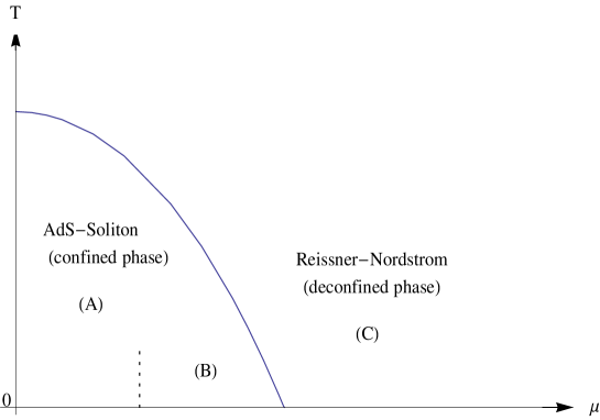
Fig. 1: A schematic phase diagram of QCD in ($\mu,T$) plane.

Recently, Eq.(1.1) has been used as a bottom-up holographic QCD model to study color superconductivity [1, 2, 9, 10] in the region (C) of Fig.1. The analysis has been performed under the assumption that the $U(1)$ gauge field is dual to the baryon number current. The model is extended up to small $N_{c}$ where $N_{c}$ is the number of colors and the authors of Ref. [2] pointed out that the color superconducting (CSC) phase could not be found for $N_{c}\geq 2$. However, the existence of the CSC phase has been pointed out when the model is improved by adding the higher derivative terms, the Gauss-Bonnet term, to Eq.(1.1) [10].

Another point to be noticed is the dotted line shown in Fig. 1. In the confined phase (A), baryons are constructed from $N_{c}$ quarks. Then, at a certain chemical potential, they are assembled as nuclear matter. The region (B) is called as the nuclear matter phase. In the previous studies, this phase has been foreseen in terms of the top-down model [11, 12, 13], based on the Sakai-Sugimoto D4/D8 model [14, 15]. In these models, baryon is introduced as an instanton which is a soliton constructed from the flavored vector mesons.

Here, based on our bottom-up holographic model (1.1), we study the nuclear matter according to the idea that it is constructed from the instanton gas. In order to provide baryons, we add $SU(N_{f})$ gauge field sector to Eq.(1.1) [11, 14, 15, 16], where $N_{f}$ is the number of flavors. Then the dilute gas of instantons is examined at finite chemical potential and at low temperature with Chern-Simons (CS) term which connects the instantons and the $U(1)$ gauge field [15]. From the model of the nuclear matter given here, we can derive the equation of state (EoS). Then it can be applied to the compact cold star (like the neutron star) to estimate the relation of the mass and the radius.

For the deconfined phase (C), up to now, some holographic models have been applied to investigate the neutron star with a quark matter core [17, 18, 19]. On the other hand, the holographic investigation of the matter in the region (B) has not been performed well to study the neutron star, particularly for the mass-radius relation. Of course, several investigations for baryons have been done with the holographic models; see Refs. [20, 21, 22, 23, 24, 25] for examples of previous studies.

In our approach, instead of solving the equations of motion, the flavored gauge fields are replaced by the instanton solution given in $R^{4}$ flat space with an instanton of size $\rho$. The solution is regarded as a trial function of the solutions of their equations of motion. Since, in our case, the instanton is embedded in a deformed 4D space of the curved 6D background space-time, then the size $\rho$ is not arbitrary, and it should be fixed at a suitable value [2, 15]. This value is determined here by minimizing the free energy of the system at $\rho=\rho_{\mathrm{min}}$. Then the other physical quantities (the free energy, the chemical potential, and others) are obtained by using this $\rho_{\mathrm{min}}$ and other parameters of the theory. As a result, the resultant free energy can be expressed as a function of $\mu$ [2]. Then through this approach, we can obtain the EoS of the instanton gas; namely the nuclear matter.

Another quantity which characterize the instanton gas is the speed of sound ($C_{s}$) of the system. We find the condition to its value as $1/2<C_{s}^{2}<1$ ; although it preserves the causality since it is smaller than unity, the lower bound is 1/2, which is large compared to that of the nuclear matter.

In this article, $SU(2)$ flavored vector fields are introduced. And the instanton-type soliton solution of the vector fields is considered as the baryon, which can be observed in the confined region as shown in Fig. 1. In the confined phase, the CSC phase is realized for $\mu>4.7$ [2]. However, when the back-reaction is considered as in the present case, this CSC phase region is replaced by the newly appeared RN deconfined phase, which becomes dominant for $\mu>1.7$ [2]. Since we are considering the baryons in the confined phase, we avoid discussing the EoS in CSC phase.

In the next section, our bottom-up model is proposed by introducing a dilute gas of instantons. In Sec. 3, we explain how to embed the instantons in the confined background metric. In Sec. 4, the free energy of the system is computed according to our method, and EoS for the instanton gas is obtained at low temperature. In Sec. 5, using the EoS, the Tolman-Oppenheimer-Volkov (TOV) equations for a compact star are solved to find the mass-radius ($M$-$R$) relation. In Sec. 6, our results are compared with the ones from nuclear physics and astronomical observations. In the final section, summary and discussions are given.

2 Bottom-up CSC model with nuclear matter

We start from the bottom-up holographic model which is proposed as YM theory with color superconducting phase. It is given by the following gravitational theory [2, 3, 4].

$$S = \int d^{d+1}\xi\sqrt{-g}\,\mathcal{L}\,,$$ (2.1)

$$\mathcal{L} = \mathcal{L}_{\mathrm{Gravity}}+\mathcal{L}_{\mathrm{CSC}}\,,$$ (2.2)

$$\mathcal{L}_{\mathrm{Gravity}} = {\cal R}+{d(d-1)\over L^{2}}\,,$$ (2.3)

$$\mathcal{L}_{\mathrm{CSC}} = -{1\over 4}F^{2}-|D_{{}_{\mu}}\psi|^{2}-m^{2}|\psi|^{2}\,,$$ (2.4)

$$F_{\mu\nu} = \partial_{\mu}A_{\nu}-\partial_{\nu}A_{\mu}\,,\quad D_{\mu}\psi=(\partial_{\mu}-iqA_{\mu})\psi\,.$$ (2.5)

This describes $(d+1)$-dimensional gravity coupled to a $U(1)$ gauge field, $A_{\mu}$, and a charged scalar field, $\psi$. Here we consider the case of $d=5$. The charge $q$ denotes the baryon number of the scalar $\psi$, and it is chosen as $q=2/N_{c}$ to represent the quark-Cooper pair formation. The mass $m$ is given to reproduce the corresponding conformal dimension of the diquark operator dual to the scalar field $\psi$ with the charge $q=2/N_{c}$. Here, we put $1/2\kappa_{6}^{2}=1$, and the dimensionful $U(1)$ gauge-coupling constant is set as unit. So the metric is dimensionless and $A_{\mu}$ has dimension one as in the (3+1)-dimensional case.

Previously, the above holographic model has been considered to be dual to the superconductor of the electric charge [3, 4] and of the $R$ charge [6]. And it was recently extended to a theory dual of the color superconductor in [1, 2, 9].

Here we add the sector of the $SU(N_{f})$ gauge fields, which is used to build the nuclear matter through the instanton configuration, which generates the baryon number in QCD. Here, the instanton configuration is deformed since it is embedded in a higher-dimensional curved space.

$$\mathcal{L} = \mathcal{L}_{\mathrm{Gravity}}+\mathcal{L}_{\mathrm{CSC}}+\mathcal{L}_{\mathrm{V}}\,,$$ (2.6)

$$\mathcal{L}_{\mathrm{V}} = -{1\over 4}{\rm tr}F^{2}_{SU(N_{f})}$$ (2.7)

where $F^{2}_{SU(N_{f})}$ denotes the 2-form $SU(N_{f})$ gauge field. The coupling constant $g_{\rm YM}^{2}$ is set as one. The mass dimension of the gauge field is taken to be one. Then, in order to pick up the coupling of the baryon number current and the instanton configuration, we add the CS term,

$$S=\int d^{d+1}x\sqrt{-g}\,\mathcal{L}+S_{\rm CS}\,.$$ (2.8)

We notice that there are two ways to proceed with the analysis based on this model since both the matter and the gravity fields are living in the same 6D spacetime. Therefore, the matter fields are not confined to special $D$-branes:

(i) So, in one way, we can solve the equations of motion of all fields, gauge fields and the gravity, in the same way. In this case, the back-reaction of the gauge fields are included in the metric.

(ii) On the other hand, it is possible to restrict our calculation to the probe approximation where the equation of motion of the matter fields are solved on a fixed background given by the solution of the Einstein equations of $\mathcal{L}_{\rm Gravity}$. This approximation is assured for the large gauge couplings.

Hereafter we proceed with the analysis according to the probe approximation (ii). The matter parts are considered as the probe of the system. So, first we fix the gravitational background by solving ${\cal L}_{\rm Gravity}$.

2.1 Instanton in $R^{4}$

Before solving the equation of motion of our model, the ansatz for the $U(1)$ gauge field and the instanton configurations for $SU(2)$ gauge fields are given. The coordinates are denoted as $(\xi^{0},\xi^{1},\xi^{2},\xi^{3},\xi^{4},\xi^{5})=(x^{0},x^{1},x^{2},x^{3},w,z)$. Then, we set the ansatz for $U(1)$ gauge field as

$$A_{b}=A_{b}(z)\delta_{b}^{0}\,.$$ (2.9)

The $SU(2)$ vector fields are set as

$$\vec{f}_{1}=F_{ab}^{i}\tau_{i}\,,$$ (2.10)

and the following ansats are imposed,

$$(\vec{f}_{1})_{ij} = Q(x^{m}-a^{m},\rho)\epsilon_{ijk}\tau^{k}\,,$$ (2.11)

$$(\vec{f}_{1})_{iz} = Q(x^{m}-a^{m},\rho)\tau^{i}\,,$$ (2.12)

where $\rho$ ($a^{m}$) denotes the instanton size (position), $\epsilon_{123z}=1$, $i,j=1,2,3$ and $m=1,\dots,4$, where $x^{4}=z$. Then the $SU(N_{f})$ vector part (2.7) is given for $N_{f}=2$ as

$$\mathcal{L}_{\mathrm{V}}=-{3\over 2}Q^{2}\left[\left({g}^{11}\right)^{2}+{g}^{11}{g}^{zz}\right]\ .$$ (2.13)

In order to see the baryon, $Q$ is given as an instanton solution in flat 4D space $\{x^{m}\}$ [15],

$$Q={2\rho^{2}\over\left((x^{m}-a^{m})^{2}+\rho^{2}\right)^{2}}\,.$$ (2.14)

However, in general, this is not a solution of our bottom-up model since this configuration is embedded in a curved space. So, here we introduce it as a trial function which is supposed to be a solution of the system under an appropriate condition. The trial function is given in our formulation such that the size parameter $\rho$ of the instanton configuration is determined to satisfy the variational principle of the energy density in our bottom-up model. We determine it by minimizing the embedded instanton energy as in Refs. [13, 15]. We notice that there is an another method giving $Q$ — including its $z$ dependence — by solving the embedding equations of motion [12]. Here we solve only for the size parameter.

According to the above strategy, we study multi-baryon state by replacing $Q(z)$ by the multi-instanton form with dilute gas approximation. Then we rewrite $Q$ as

$$Q^{2}=\sum_{i}^{N_{\mathrm{I}}}{4\rho^{4}\over\left((x^{m}-a^{m}_{i})^{2}+\rho^{2}\right)^{4}}\,,$$ (2.15)

where the overlap among the instantons are suppressed in obtaining $Q^{2}$. This point is checked for our solutions.

In the case of the flat space, in $R^{4}$, we find the energy density as a sum of each single instanton,

$$\int d^{4}\xi^{m}Q^{2} = 2N_{\mathrm{I}}\int_{0}^{\infty}dz\bar{q}(z)^{2}\,$$ (2.16)

$$= {2\pi^{2}\over 3}N_{\mathrm{I}}\,,$$

where

$$\bar{q}^{2}={\pi^{2}\rho^{4}\over 2(z^{2}+\rho^{2})^{5/2}}\,$$ (2.17)

for the case of dilute gas, where interactions between instantons are neglected. Then the result is given by one instanton “mass” times its number $N_{\mathrm{I}}$.

In the present case, the instantons are embedded in a curved space. The metrics are functions of the coordinate $z$. This implies that the state of the baryon is affected dynamically by the gluons. In other words, the baryon is stable when it is embedded in the background corresponding to the confined phase. Furthermore, these baryons would construct a nuclear matter like the neutron star as we see below.

3 Low temperature confined phase and the fourth coordinate $z$

We suppose the nuclear matter would be the gas of instantons made up of the $SU(2)$ gauge fields in the confined phase. The spacetime background solution, which is dual to the low temperature confined phase, is given from $\mathcal{L}_{\mathrm{Gravity}}$ at low temperature as the AdS-soliton solution. It is obtained as

$$ds^{2}=r^{2}(\eta_{\mu\nu}dx^{\mu}dx^{\nu}+f(r)dw^{2})+{dr^{2}\over r^{2}f(r)}\,,$$ (3.1)

where

$$f(r)=1-\left({r_{0}\over r}\right)^{5}\,,\quad r_{0}={2\over 5R_{w}}\,,$$ (3.2)

and $2\pi R_{w}$ denotes the compactified length of $w$, which denotes the coordinate of the compact $S^{1}$. We notice that this solution is also a back-reacted one when the $SU(2)$ gauge fields are set to be zero. In this case, the phase diagram in the $\mu$-$T$ plane is given in Ref. [2].

Here we restrict the region of the parameters, $T$ and $\mu$, to the confined phase. In fact, under the configuration (3.1), one finds a linear potential between quark and antiquark by evaluating the Wilson loop [26]. Hence the vacuum stays in the confined phase, and the instanton number is identified with the baryon number. Then, in this confined phase, we can examine the nuclear matter through the gas of instantons.

3.1 Coordinate $z$ and embedding of instanton

In proceeding the analysis mentioned above, it is necessary to choose the coordinate $z$ carefully. For example, we may choose the four coordinates to make the instanton as,

$$(\xi^{0},\xi^{1},\xi^{2},\xi^{3},\xi^{4})=(x^{0},x^{1},x^{2},x^{3},r)\,,$$ (3.3)

namely as $z=r$. In this case, using $(\ref{LV-2})$ and $(\ref{Soliton})$, we have

$$S_{\rm V} = \int d^{6}\xi\sqrt{-g}\,\mathcal{L}_{\rm V}\,,$$ (3.4)

$$= \int dx^{0}dx^{1}dx^{2}dx^{3}dwdr~{}r^{4}\left(-{3\over 2}Q^{2}\left[{1\over r^{4}}+f(r)\right]\right)\,$$

$$= \int dx^{0}dwdr~{}r^{4}\left(-{3\over 2}2N_{\rm I}\bar{q}^{2}\left[{1\over r^{4}}+f(r)\right]\right)\,$$

$$= N_{\rm I}\int dx^{0}dwdr~{}r^{4}\left(-{3\over 2}{\pi^{2}\rho^{4}\over(r^{2}+\rho^{2})^{5/2}}\left[{1\over r^{4}}+f(r)\right]\right)\ .$$

Here we find a logarithmic divergence in the integration over $r$. It is understood as follows:

$$S_{\rm V} \propto \int^{\infty}_{r_{0}}dr~{}r^{4}\left(-{3\over 2}{\pi^{2}\rho^{4}\over(r^{2}+\rho^{2})^{5/2}}\left[{1\over r^{4}}+f(r)\right]\right)\,$$ (3.5)

$$\sim\atop{}_{r\to\infty} \int^{\infty}dr\left(-{3\over 2}{\pi^{2}\rho^{4}\over r}\right)\sim-{3\over 2}{\pi^{2}\rho^{4}}\log(\infty)\,.$$

This fact implies that we should reset $z$ to other coordinate which leads to a finite energy density of the instanton.

A clue to finding such coordinate is seen in the top-down model of D4/D8 model [2, 14, 15]. In the case of the top-down model, D8-flavor brane is embedded in a set of special coordinates, which provide a flat space of $r$-$w$ plane near the point $r=r_{0}$ by avoiding a conical singularity. This is performed in the present case by changing the coordinates from $(r,w)$ to $(z,\theta)$ as,

$$r^{5} = r_{0}^{5}+r_{0}^{3}z^{2}\equiv k\,,$$ (3.6)

$$\theta = {5\over 2}w\,.$$ (3.7)

In fact, in this case, the two dimensional part of (3.1) is rewritten as

$$ds^{2}_{(2)} = r^{2}f(r)dw^{2}+{dr^{2}\over r^{2}f(r)}\,$$ (3.8)

$$= {4\over 25}\left({r_{0}\over r}\right)^{3}\left({dz^{2}\over r^{2}}+z^{2}d\theta^{2}\right)\,.$$

The second equation shows that the two dimensional metric is the polar coordinate of 2D flat space. Hereafter, we take $r_{0}=1$ for simplicity as in the top-down case. In this coordinate, the bulk 6D metric is written as

$$ds^{2}=k^{2/5}\eta_{\mu\nu}dx^{\mu}dx^{\nu}+{4\over 25}k^{-3/5}(k^{-2/5}dz^{2}+z^{2}d\theta^{2})\,,$$ (3.9)

where $k=1+z^{2}$.

Here, noticing $\sqrt{-g}=(4/25)z$, the energy of the embedded instantons is given as

$$S_{\rm V} = \int dx^{0}dx^{1}dx^{2}dx^{3}dz~{}{4\over 25}z\left(-{3\over 2}Q^{2}\left[k^{-4/5}+{25\over 4}k^{3/5}\right]\right)\,$$ (3.10)

$$= N_{\rm I}\int dx^{0}dz~{}{4\over 25}z\left(-{3\over 2}{\pi^{2}\rho^{4}\over(z^{2}+\rho^{2})^{5/2}}\left[k^{-4/5}+{25\over 4}k^{3/5}\right]\right)\,,$$

where the factor $\int\!d\theta=2\pi$ is absorbed to the gauge coupling constant. We can assure the finiteness of the $z$ integration of the above action.

3.2 CS term

The baryon number is given by

$$N_{\mathrm{B}}={1\over 32\pi^{2}}\int d^{3}xdz\epsilon^{m_{1}\cdots m_{4}}{\rm tr}(F_{m_{1}m_{2}}F_{m_{3}m_{4}})\,.$$ (3.11)

Then the coupling of $A_{0}$ to the baryon number is given by the following CS term,

$$S_{\rm CS} = \kappa_{\rm CS}\epsilon^{m_{1}\cdots m_{4}}\int d^{4}x~{}dz~{}A_{0}{\rm tr}(F_{m_{1}m_{2}}F_{m_{3}m_{4}})\,$$ (3.12)

$$= 24\kappa_{\rm CS}\int d^{4}xdz~{}A_{0}Q^{2}\,$$

$$= 48n\kappa_{\rm CS}\int d^{4}xdz~{}A_{0}\bar{q}^{2}\,,$$

where

$$n={N_{\rm I}\over V_{3}}\,,\quad V_{3}=\int d^{3}x=\int dx^{1}dx^{2}dx^{3}.$$ (3.13)

4 Effective action and the size of the instanton

The matter action with embedded instantons is obtained here as

$$S_{\rm matter} = \int d^{6}\xi\sqrt{-g}\,\left(-{1\over 4}F^{2}-{1\over 4}{\rm tr}F^{2}_{SU(2)}\,\right)+S_{\rm CS}\,$$ (4.1)

$$= \int d^{4}xdz\left({1\over 2}zk^{3/5}{A_{0}^{\prime}}~{}^{2}-nz{12\over 25}\bar{q}^{2}\left[k^{-4/5}+{25\over 4}k^{3/5}\right]+nn_{0}A_{0}\bar{q}^{2}\right)\,,$$

where $A_{0}^{\prime}=\partial_{z}A_{0}(z)$, and $n_{0}=48\kappa_{\rm CS}$. In order to estimate this action, we solve the equation of motion of $A_{0}(z)$. It is obtained as

$$-\partial_{z}\left(zk^{3/5}A_{0}^{\prime}\right)+nn_{0}\bar{q}^{2}=0\,.$$ (4.2)

Then we have

$$zk^{3/5}A_{0}^{\prime}=\bar{d}={\pi^{2}\over 6}nn_{0}{2z^{3}+3z\rho^{2}\over(z^{2}+\rho^{2})^{3/2}}+c\,.$$ (4.3)

Here, $c$ denotes an integration constant of Eq. (4.2) over $z$. We take $c=0$ to set as $\bar{d}(z=0)=0$. Due to this condition, the matter action, $S_{\rm matter}$ of (4.1), is written as

$$S_{\rm matter}=\int d^{4}x\left\{\mu\bar{Q}-\int dz\left({\bar{d}~{}^{2}\over 2zk^{3/5}}+nz{12\over 25}\bar{q}^{2}\left[k^{-4/5}+{25\over 4}k^{3/5}\right]\right)\right\}\,,$$ (4.4)

where the chemical potential $\mu$ and the charge density $\bar{Q}\equiv{\bar{d}(\infty)}$ are given as

$$\mu = A_{0}(\infty)=\int_{z_{1}}^{\infty}dz{\bar{d}\over zk^{3/5}}+A_{0}(z_{1})\,$$ (4.5)

$$= \int_{z_{1}}^{\infty}dz{\bar{d}\over zk^{3/5}}\,,$$

$$\bar{Q} = \bar{d}(\infty)={\pi^{2}\over 3}nn_{0}\,,$$ (4.6)

where $z_{1}$ is an arbitrary positive value and $A_{0}(z_{1})$ is set as

$$A_{0}(z_{1})=0\,,$$ (4.7)

which is the boundary condition in solving the differential equation of $A_{0}(z)$, Eq. (4.3).
Then the free energy density ${\cal E}$ of the instanton system is given as

$$S_{\rm matter} = -\int d^{5}\xi~{}~{}{\cal E}(\rho,\mu)\,$$ (4.8)

$${\cal E}(\rho,\mu) = \int dz\left({\bar{d}~{}^{2}\over 2zk^{3/5}}+nz{12\over 25}\bar{q}^{2}\left[k^{-4/5}+{25\over 4}k^{3/5}\right]\right)-\mu\bar{Q}\,$$ (4.9)

4.1 Size of instanton

The free energy density ${\cal E}(\rho,\mu)$ in (4.9) is given as a function of $\rho$ for fixed $n,n_{0},z_{1}$. Then we find the value of $\rho=\rho_{\rm min}$ where ${\cal E}(\rho,\mu(\rho))$ takes its minimum for a set of $(n,n_{0},z_{1})$; for this $\rho_{\rm min}$, $\mu$ and ${\cal E}(\rho,\mu)$ are determined. Repeating this procedure by changing only the value $n$ of the set $(n,n_{0},z_{1})$, we find different $\rho_{\rm min}$. As a result, we obtain the relation between $\mu$ and ${\cal E}(\rho,\mu)$.

We notice that the results obtained in this way depend on the other two parameters $(n_{0},z_{1})$. We give a comment related to the parameter $z_{1}$. For $z_{1}=0$, we have a problem that the values of $\mu$ and ${\cal E}$ at $\rho=0$ are divergent,

$$\mu|_{\rho\to 0} = \int_{0}^{\infty}dz{\bar{d}(\infty)\over zk^{3/5}}\,$$ (4.10)

$$\sim\atop{}_{z\to 0} \bar{d}(\infty)\int_{0}{dz\over z}\to+\infty\,,$$

$${\cal E}(\rho=0,\mu)| \sim\atop{}_{z\to 0} \int_{0}dz\left(-{\bar{d}(\infty)^{2}\over 2zk^{3/5}}\right)\to-\infty.$$ (4.11)

In the present model these divergences are evaded by setting $z_{1}$, the lower bound of $z$, at a finite value. On the other hand, in the case of the top-down model [13], there are no such divergences. In fact, we can see that $\mu$ is finite even if $\rho$ is zero for $z_{1}=0$. Therefore, we expect the existence of some improvement of the present bottom-up model to resolve the above divergences. Here, this point remains as an open problem, and $z_{1}$ is introduced as a simple cutoff parameter for the above undesirable infrared divergences.

4.2 EoS for nuclear matter

By giving $n,n_{0},z_{1}$, (which are the parameters of the present bottom-up model), $\mu(\rho)$ and ${\cal E}(\rho)$ are calculated according to the Eqs. (4.5) and (4.9) as the functions of $\rho$. Then a minimum point of ${\cal E}(\rho)$ is found at $\rho=\rho_{\rm min}$. Thus we can obtain ${\cal E}(\rho_{\rm min})$ and $\mu(\rho_{\rm min})$ for the given parameters $n,n_{0},z_{1}$.

Repeating this procedure by changing only $n$ with $(n_{0},z_{1})$ fixed, then we get the relationship of $\mu$ and ${\cal E}$. From this relationship we obtain the EoS of the instanton gas as mentioned above.

Table 1: EoS of nuclear system at low temperature for $n_{0}=1.5,z_{1}=0.1$, and

$v_{\rm min}={4\over 3}\pi\rho_{\rm min}^{3}n$.

$n$	$\mu(\rho_{\rm min})$	${\cal E}(\rho_{\rm min})$	$\rho_{\rm min}$	$v_{\rm min}$
0.005	0.0688	0.00031	0.01	2.09 $\times 10^{-8}$
0.01	0.138	0.0000393	0.02	3.35$\times 10^{-7}$
0.015	0.209	-0.00022	0.03	1.70$\times 10^{-6}$
0.02	0.275	-0.00178	0.04	5.36 $\times 10^{-6}$
0.03	0.411	-0.00829	0.06	2.75 $\times 10^{-5}$
0.05	0.68	-0.0368	0.09	1.52$\times 10^{-4}$
0.1	1.335	-0.2075	0.13	9.2 $\times 10^{-4}$

In Table 1, we show a resultant example of such calculations for $n_{0}=1.5,z_{1}=0.1$. The regions of the calculations are restricted to the region for $\mu<1.7$ [2]. On the other hand, the pressure $p$, which is given by $p=-{\cal E}$, of the instanton gas is negative for $\mu<\mu_{c}\sim 0.17$. So in this region, the gas is in an undesirable phase as a nuclear matter considered here.

Thus we find that the stable nuclear matter exists in the region, $1.7>\mu>\mu_{c}\sim 0.17$. In this region of the nuclear matter, its dilute gas picture is reasonable since $v_{\rm min}\sim O(10^{-4})\ll 1$, where $v_{\rm min}={4\over 3}\pi\rho_{\rm min}^{3}n$ indicates the volume which is occupied by instantons in a unit 3D volume.

Here we proceed the analysis, and we can arrive at the following approximate formula

$$p=a\mu(\mu-\mu_{c})\,,$$ (4.12)

where $a=0.13$ and $\mu_{c}=0.17$ (See Fig. 2). Then using (4.12). the energy density is given at $T=0$ as [18]

$${\epsilon}=\mu q-p=\mu{\partial p\over\partial\mu}-p=a\mu^{2}\,,$$ (4.13)

and the speed of sound is obtained as

$$C_{s}^{2}={\partial p\over\partial\epsilon}={\partial p/\partial\mu\over\partial\epsilon/\partial\mu}=1-{\mu_{c}\over 2\mu}\,.$$ (4.14)

This leads to the following bound of $C_{s}^{2}$,

$${1\over 2}<C_{s}^{2}<1\,.$$ (4.15)

We notice that the lower bound $1/2$ is fairly large comparing to that of the ordinary nuclear matter. We should however notice that the constraint (4.15) for $C_{s}^{2}$ comes from the formula (4.12), which is an approximate formula available at small $\mu$. It is possible to improve (4.12) by adding correction terms of higher powers of $\mu$. For example, by adding a term like $\mu^{4}$, we can find a new formula, $p=a^{\prime}\mu(\mu-\mu_{c}^{\prime})+b^{\prime}\mu^{4}$ with appropriate values for the parameters, $a^{\prime},\mu_{c}^{\prime},b^{\prime}$. In this case, we can see that the maximum value of $C_{s}$ is realized at $\mu$ smaller than 1 and its maximum value is suppressed from 1, then it decreases to $C_{s}=1/\sqrt{3}$ in the large $\mu$ region. However, as we can see, the correction term of $\mu^{4}$ becomes small in the small $\mu$ region. Then it is difficult to suppress largely the lower bound 1/2. We find a small value of sound speed in region of $0<C_{s}^{2}<1/2$ for $\mu<\mu_{c}$, where $\mu_{c}(\neq\mu_{c}^{\prime})$ denotes the critical point and it satisfies $p(\mu_{c})=0$. In this region of $\mu$, however, the pressure $p$ is negative, then the instanton gas cannot make a nucleon matter like a star. This implies that our model cannot cover the low-density part of the normal nuclear matter, in which the sound speed decreases to zero from its upper bound $(1/\sqrt{3})$. How to overcome this point remains as a future problem.

In this sense, the nuclear matter given here might be a special one. Our model is considered in a restricted region of density or $\mu$, $\mu_{c}<\mu<1.7$, where 1.7 denotes the transition point to the deconfined RN phase. Therefore, we continue our analysis by using a simple model with (4.12) and (4.13), then we arrive at the EoS of the nuclear matter given as the instanton gas. It is written as,

$$p=\epsilon-\sqrt{a\epsilon}\,\mu_{c}\,.$$ (4.16)

Fig. 2: $p=-{\cal E}(\mu)$ versus $\mu$ at stable instanton size $\rho_{\rm min}$ near phase transition point $\mu_{c}=0.17$. The solid curve denotes the numerical calculations, and the dotted curve represents $p=0.13\mu(\mu-\mu_{c})$.

4.3 Alternative approach to find EoS

In the present scheme, the free energy density (4.9) takes $n$, $n_{0}$, $\rho$, and $z_{1}$ as independent variables. Among them, $n_{0}$ is an intrinsic parameter of the theory and $\rho$ is determined dynamically such that $\mathcal{E}$ takes its minimum value, while $z_{1}$ is set to be a plausible value for the moment. The free energy density is expanded in a power series of $n$,

$$\mathcal{E}(n,\rho,n_{0},z_{1})=n\,c_{1}(\rho)-n^{2}n_{0}^{2}\,c_{2}(\rho,z_{1})\ ,$$ (4.17)

in which

$$c_{1}(\rho) = \frac{12}{25}\frac{\pi^{2}\rho^{4}}{2}\int_{0}^{\infty}\!\!dz\,\frac{z}{(\rho^{2}+z^{2})^{5/2}}\left[(1+z^{2})^{-4/5}+\frac{25}{4}(1+z^{2})^{3/5}\right]\ ,$$ (4.18)

$$c_{2}(\rho,z_{1}) = \left(\frac{\pi^{2}}{3}\right)^{2}\int_{0}^{\infty}\!\!dz\,\frac{1}{(1+z^{2})^{3/5}}\left[\frac{1}{2}\frac{2z^{2}+3\rho^{2}}{(\rho^{2}+z^{2})^{3/2}}-\frac{1}{8}\frac{z(2z^{2}+3\rho^{2})^{2}}{(\rho^{2}+z^{2})^{3}}\right]$$ (4.19)

$$\hskip 36.135pt-\left(\frac{\pi^{2}}{3}\right)^{2}\!\int_{0}^{z_{1}}\!dz\,\frac{1}{(1+z^{2})^{3/5}}\,\frac{1}{2}\,\frac{2z^{2}+3\rho^{2}}{(\rho^{2}+z^{2})^{3/2}}\ .$$

In order to change the independent variable from $n$ to $\mu$, we notice that $\mu$ can be written as

$$\mu(n,\rho,n_{0},z_{1})=nn_{0}\,h(\rho,z_{1})$$ (4.20)

with

$$h(\rho,z_{1})=\frac{\pi^{2}}{6}\,\int_{z_{1}}^{\infty}\!dz\,\frac{1}{(1+z^{2})^{3/5}}\,\frac{2z^{2}+3\rho^{2}}{(\rho^{2}+z^{2})^{3/2}}\ .$$ (4.21)

Now, eliminating $n$ by (4.20), the free energy density is rewritten as

$$\mathcal{E}=-\frac{c_{2}(\rho,z_{1})}{(h(\rho,z_{1}))^{2}}\,\mu^{2}+\frac{c_{1}(\rho)}{n_{0}h(\rho,z_{1})}\,\mu\ .$$ (4.22)

From Eq. (4.22) one finds that the coefficients ($a$ and $b$) and the critical chemical potential ($\mu_{c}$) are given by

$$a=\frac{c_{2}(\rho,z_{1})}{h(\rho,z_{1})^{2}}\ ,\qquad b=\frac{c_{1}(\rho)}{n_{0}\,h(\rho,z_{1})}\ ,\qquad\mu_{c}=\frac{c_{1}(\rho)\,h(\rho,z_{1})}{n_{0}\,c_{2}(\rho,z_{1})}\ .$$ (4.23)

Given $\mu$, $z_{1}$, and $n_{0}$, the minimum point of $\mathcal{E}$ (i.e., the maximum point of $p$) in the $\rho$ space can be sought numerically.

The minimum energy point depends on the variable which is taken fixed. Actually, two types of differential coefficients have different values as

$$\left(\frac{\partial\mathcal{E}}{\partial\rho}\right)_{\!n}-\left(\frac{\partial\mathcal{E}}{\partial\rho}\right)_{\!\mu}=\left(\frac{\partial\mathcal{E}}{\partial\mu}\right)_{\!\rho}\left(\frac{\partial\mu}{\partial\rho}\right)_{\!n}=-\left(\frac{\partial\mathcal{E}}{\partial n}\right)_{\!\rho}\left(\frac{\partial n}{\partial\rho}\right)_{\!\mu}\ .$$ (4.24)

At the point $\rho=\rho_{\mathrm{min}}$ such that $(\partial\mathcal{E}/\partial\rho)_{n}=0$, it holds that

$$\left(\frac{\partial\mathcal{E}}{\partial\rho}\right)_{\!\mu}=-\left(\frac{\partial\mathcal{E}}{\partial\mu}\right)_{\!\rho}\left(\frac{\partial\mu}{\partial\rho}\right)_{\!n}=(-b+2a\mu)nn_{0}\,h_{\rho}(\rho,z_{1})\ .$$ (4.25)

In (4.25), one finds that

$$h_{\rho}(\rho,z_{1})~{}\equiv~{}\frac{\partial h(\rho,z_{1})}{\partial\rho} = -\frac{\pi^{2}}{2(2a_{0})}\int_{z_{1}}^{\infty}\!dz\,\frac{1}{(1+z^{2})^{3/5}}\,\frac{\rho^{3}}{(\rho^{2}+z^{2})^{5/2}}<0\ ,$$ (4.26)

$$-b+2a\mu = a(\mu-\mu_{c})+a\mu>0\ ,$$ (4.27)

in the present situation, i.e., $a>0$ and $\mu>\mu_{c}$. Therefore, we conclude that

$$\left(\frac{\partial\mathcal{E}}{\partial\rho}\right)_{\!\mu}<0\quad\hbox{(at $\rho=\rho_{\mathrm{min}}$)}\ .$$ (4.28)

This means that the minimum energy point along an $n$-fixed curve has much lower energy points towards the $\rho$-increasing direction with $\mu$ being kept constant. However, the problem is whether the minimum energy significantly depends on the fixed variable or not.

To estimate the difference between the two types of minimum energies, one should continue numerical calculations on $\mathcal{E}$ from $\rho_{\mathrm{min}}$ by fixing $\mu$ and by increasing $\rho$ until one finds another minimum energy density $\mathcal{E}^{\prime}_{\mathrm{min}}$. In the range of $0.015\leq\rho\leq 0.1$ according to Table 1, the calculations make the difference of the minimum energies explicit quantitatively such as $(\mathcal{E}^{\prime}_{\mathrm{min}}-\mathcal{E}_{\mathrm{min}})/\mathcal{E}_{\mathrm{min}}\lesssim 0.028$.

We may consider that such differences do not affect characteristic features of EoS, and we again employ $n$ as the independent variable of $\mathcal{E}$ in the succeeding sections.

5 TOV equation and $M$-$R$ relation of neutron star

The TOV equations for a star with the mass $m$, and $p$ at the radius $r$ in the star are given as,

$${dp\over dr} = -G(\epsilon+p){m+4\pi r^{3}p\over r(r-2Gm)}\,,$$ (5.1)

$${dm\over dr} = 4\pi r^{2}\epsilon\,.$$ (5.2)

Here, $G$ denotes the gravitational constant. They can be solved by using the EoS given in (4.16) with the boundary condition, $p(r=0)=p_{c}$ and $m(r=0)=0$. Solving these equations, we obtain the mass of the star, $M=m(R)$, and its radius $R$, where $R$ is defined by $p(R)=0$.

Fig. 3: Plot of the neutron mass $M(R)$ (in unit of solar mass $M_{\odot}$) versus the radius $R$ for $p=\epsilon-\sqrt{a\epsilon}\mu_{c}$ (or $p=a\mu(\mu-\mu_{c})$), $\mu_{c}=0.17$ and $a=0.13$.

In order to obtain the numerical results with dimensionful quantities, we must adjust the scale parameters for each dimensionful quantities ($\tilde{x}$). To do so, the above TOV equations are rewritten by using the dimensionless quantities as [19]

$${d{\tilde{p}}\over d{\tilde{r}}} = -B({\tilde{\epsilon}}+{\tilde{p}}){{\tilde{m}}+4\pi A{\tilde{r}}^{3}{\tilde{p}}\over{\tilde{r}}({\tilde{r}}-2B{\tilde{m}})}\,,$$ (5.3)

$${d{\tilde{m}}\over d{\tilde{r}}} = 4\pi A{\tilde{r}}^{2}{\tilde{\epsilon}}\,,$$ (5.4)

where

$$A={r_{0}^{3}\epsilon_{0}\over m_{0}}\,,\quad B={Gm_{0}\epsilon_{0}\over p_{0}r_{0}},$$ (5.5)

and the various variables ($x$) are replaced by the dimensionless quantities ($\tilde{x}$) by using its typical dimensionful value $x_{0}$ as $x=x_{0}{\tilde{x}}$. For example, we rewrite as $p=p_{0}{\tilde{p}}$.

Here we give a comment on the replacement, $\epsilon=\epsilon_{0}\tilde{\epsilon}$ and how $\epsilon_{0}$ is determined. In order to solve the TOV equation, $\epsilon(r)$ in the equation is replaced using the Eq. (4.16) as a function of $p(r)$,

$$\epsilon={a\mu_{c}^{2}\over 4}\left(1+\sqrt{1+{4p\over a\mu_{c}^{2}}}\right)^{2}\,.$$ (5.6)

Similar to the above, we introduce the dimensionless quantities as $a=a_{0}\tilde{a}$, $\mu_{c}=\mu_{0}\tilde{\mu}_{c}$, and

$$\epsilon=\epsilon_{0}\tilde{\epsilon}\,,$$ (5.7)

by imposing reasonable conditions

$$\quad\epsilon_{0}=p_{0}=a_{0}\mu_{0}^{2}\,.$$ (5.8)

Then in Eqs. (5.3) and (5.4), we find

$$\tilde{\epsilon}={\tilde{a}\tilde{\mu}_{c}^{2}\over 4}\left(1+\sqrt{1+{4\tilde{p}\over\tilde{a}\tilde{\mu}_{c}^{2}}}\right)^{2}\,,$$ (5.9)

where we put the dimensionless number as $\tilde{a}\tilde{\mu}_{c}^{2}=0.13\times 0.17^{2}=3.76\times 10^{-3}$.

Then the solutions of (5.3) and (5.4) with $A=B=1$ are equal to the one of (5.1) and (5.2) with $G=1$. Then the solution of the latter equations are translated to the one of the former ones as shown in Fig. 3; it is given for $r_{0}=3.0$ km in natural units. In this case, we find $m_{0}=2.03M_{\odot}$ and $\epsilon_{0}^{1/4}=0.896$ GeV, which provides physical units to the quantities given in the Table 1. For example, the energy density of the center of the star, whose mass is about two solar mass, is given by 0.00242 GeV⁴. This is about twice as large as the one of the normal nuclear matter.

We can see that the radius and the mass increase with increasing $p_{c}$, the central value of the pressure. The resultant curve rotates anticlockwise toward the smaller radius in the large mass region. However from the point II to the point III in Fig. 3, the state would be unstable since $\partial M(\epsilon_{c})/\partial\epsilon_{c}<0$ [19] . On the other hand, in the region from I to II, we can see the behavior $\partial M(\epsilon_{c})/\partial\epsilon_{c}>0$. Thus, the results given here indicate the possibility of the existence of a star with $(M,R)\sim(2M_{\odot},10\ \mathrm{km})$.

6 Comparison with the observational data

There are some important observational data which can constrain the theoretical EoS. We now have the following at least three important constraints for the $M$-$R$ relation;

1. Two solar mass ($2M_{\odot}$) neutron star observation from the Shapiro delay measurement [29, 30].

2. Radius constraint from GW170817 via the gravitational wave observation. The actual constraint is $9.0~{}\mathrm{km}<R<13.6~{}\mathrm{km}$ for $M=1.4M_{\odot}$ [31, 32, 33].

3. The upper bound of $M$ for cold spherical neutron stars which is estimated from no detection of relativistic optical counterpart in the analysis of GW170817. The actual limit is estimated as the range $2.15M_{\odot}-2.26M_{\odot}$ [34].

To support $2M_{\odot}$ neutron stars in the theoretical calculation, we need a sufficiently stiff EoS and it is closely related to the large value of the speed of sound. Then, the pressure of matter in the inner neutron star core should be large. From the second constraint – the radius is relatively small in the moderate $M$ region – it requires that the pressure of the matter in the outer neutron core should be relatively small. It is interesting that our bottom-up model is quite simple, but our EoS can manifest the $2M_{\odot}$ constraint and the restriction that the $M$-$R$ curve must go through $9.0<R<13.6$ around $M\sim 1.4M_{\odot}$. However, too stiff EoS is not preferable because of the third constraint. Unfortunately, the maximum mass $M_{\mathrm{max}}$ overshoots the $2.15M_{\odot}-2.26M_{\odot}$ constraint, but we can expect that there are some phase transitions at high density such as the chiral, deconfined, and color superconducting phase transitions which we do not consider in this study. Then, EoS can be softer than the present one at high density and thus $M_{\mathrm{max}}$ should be smaller than the present value. Particularly, EoS becomes soft if there is a first-order phase transition; for example, see Ref. [35].

It should be noted that the above constrains can restrict the large and moderate $M$ regions, but the lower $M$ region is not restricted so much. Of course, there are several nuclear theoretical EoS and thus we can qualitatively discuss the lower $M$ region where the low density part of EoS dominates the $M$-$R$ curve. With our EoS, the $M$-$R$ curve flows down to the bottom left, but several $M$-$R$ curves with different EoS flow down to the bottom right. This result may be induced from the fact that our $C_{s}^{2}$ cannot be less than $1/2$ even in the sufficiently low-density region. Such behavior is similar to the $M$-$R$ curves obtained with EoS proposed in Ref. [36]; the actual behavior of the curves can be seen in Refs. [37, 38] denoted as “SQM1-3” and these EoS which contain the quark matter make self-bounded neutron stars which do not have minimum masses. The tendency of the $M$-$R$ curves in the small $M$ region in our model may be modified when we suitably introduce “interactions” to the present model because we employ the dilute instanton gas approximation; the baryonic contribution can be expected to have relatively strong effects on the EoS at low density. In addition, we here use the dilute gas of the instanton of the $SU(2)$ gauge field and thus the number of the flavor is considered as two; the system contains the up and down quarks and thus there is no strange quark. This may introduce the unclearness to the present $M$-$R$ curves because the EoS will be softer than the present one if hyperons appear in the system; since the core of the neutron star is very dense, the hyperon degree of freedom can join the game as the baryonic mode in addition to nucleons. This softening problem induced by the hyperons is the so-called hyperon puzzle which is a long standing problem in the study of the neuron stars with EoS; see Ref. [39] as an example. To discuss this problem in the present bottom-up holographic model, we must consider differences between the light quarks and the strange quark, interactions and bound states more deeply. In the present study, we consider the simple symmetric nuclear matter because the difference between the flavors and effects of the electrons are difficult to include in the model at present. Therefore, the inclusion of the effects such as the beta equilibrium and charge neutrality are left for our future work.

7 Summary and discussions

In this paper, we have studied cold nuclear matter and its equation of state (EoS) based on the six-dimensional holographic model, which was investigated previously to realize the color superconducting phase of QCD. The nuclear matter was introduced as a dilute gas of deformed instantons in the AdS soliton background. The instantons are electric-charge neutral and they are made up of the $SU(2)$ gauge fields; the action includes the Chern-Simons term as well as the kinetic term. Owing to the energy balance between these two terms in the action, the size of the instanton can be determined for fixed parameters of the model. As the result, the EoS for nuclear matter, i.e., pressure as a function of energy density, is obtained. Through the evaluation of the instanton size, it turns out that the number of instantons in a unit volume is very small so that our dilute gas picture is consistent. Furthermore, there exists a critical value for the chemical potential below which the pressure becomes negative. The EoS obtained here is very stiff because the speed of sound $C_{s}^{2}>\frac{1}{2}$. As discussed in the Sec. 4.2, this constraint is reduced to our simplified form of the pressure, $p(\mu)$. The lower bound 1/2 can be suppressed when the functional form of $p(\mu)$ is modified.

Here, we however consider an EoS which is obtained from the simplified $p(\mu)$ to see the characteristic properties of our model. Then, we applied the simplified EoS to solve the Tolman-Oppenheimer-Volkov equations for a compact star numerically and found the mass-radius ($M$-$R$) relationship. The curve is somewhat similar to the one for strange quark matter in Refs. [36, 38] and we provided a certain interpretation for that. Our result is compared with the observational data and it is seen that the maximum mass overshoots the current constraint since our EoS for the nuclear matter is very stiff. This might suggest that we have more phases such as quark matter, which softens the current EoS, than that of the nuclear matter. As we have shown in the Sec. 4, our dilute gas picture is appropriate. There is a reason why we could achieve two solar mass neutron star in spite of the diluteness of the instanton gas. In our approach, it might be possible that the mass of an instanton is very heavy compared with an ordinary nucleon, which is a specific property in holographic QCD since the nucleon mass is proportional to the number of colors $N_{c}$. So far we have no definite answer and this is a future issue.

In order to improve our current study, several ingredients are taken into account. One is to go beyond the dilute gas approximation of instantons. By doing this, our EoS is modified and eventually the $M$-$R$ curve might be changed so as to be more consistent with the observational data. The other is to study whether the system enjoys the phase transition from nuclear matter to (perhaps color superconducting) quark matter at higher baryon density. If such a phase transition is present, the EoS gets soften and the resultant $M$-$R$ curve could be modified. Furthermore, it will be interesting to extend our current study into the case with hyperon degrees of freedom. To this end, the holographic treatment of heavy-light meson system (for instance, see [40]) must be instructive. These issues will be considered in the future.

References

- [1] Pallab Basu, Fernando Nogueira, Moshe Rozali, Jared B. Stang, Mark Van Raamsdonk, “Towards A Holographic Model of Color Superconductivity”, New J.Phys.13:055001,2011, [arXiv:1101.4042 [hep-th]].
- [2] Kazuo Ghoroku, Kouji Kashiwa, Yoshimasa Nakano, Motoi Tachibana, Fumihiko Toyoda “Color Superconductivity in Holographic SYM Theory”, Phys. Rev. D 99, 106011 (2019), arXiv:1902.01093[hep-th]:
- [3] Steven S. Gubser, “Breaking an Abelian gauge symmetry near a black hole horizon”, Phys.Rev.D78:065034,2008, arXiv:0801.2977 [hep-th].
- [4] Sean A. Hartnoll, Christopher P. Herzog, Gary T. Horowitz, “Building an AdS/CFT superconductor”, Phys. Rev. Lett. 101.031601, [Xiv:0803.3295 [hep-th]];
- [5] S. A. Hartnoll, C. P. Herzog and G. T. Horowitz, “Holographic Superconductors,” JHEP 0812, 015 (2008) [arXiv:0810.1563 [hep-th]].
- [6] Tatsuma Nishioka, Shinsei Ryu, Tadashi Takayanagi, “Holographic Superconductor/Insulator Transition at Zero Temperature”, JHEP 1003:131,2010, JHEP03(2010)131, [arXiv:0911.0962 [hep-th]].
- [7] N. Iqbal, H. Liu, M. Mezei et al., “Quantum phase transitions in holographic models of magnetism and superconductors,” Phys. Rev. D82, 045002 (2010). [arXiv:1003.0010 [hep-th]].
- [8] Andrew Chamblin, Roberto Emparan, Clifford V. Johnson, Robert C. Myers, “Charged AdS Black Holes and Catastrophic Holography”, 10.1103/PhysRevD.60.064018, hep-th/9902170:
- [9] Kazem Bitaghsir Fadafan, Jesus Cruz Rojas, Nick Evans, “A Holographic Description of Colour Superconductivity”, Phys. Rev. D 98, 066010 (2018), [arXiv:1803.03107 [hep-ph]].
- [10] Cao H. Nam, “A more realistic holographic model of color superconductivity with higher derivative corrections”, arXiv:2101.00882[hep-th]
- [11] Oren Bergman, Gilad Lifschytz, Matthew Lippert, “Holographic Nuclear Physics”, JHEP0711:056,2007, arrXiv:0708.0326 [hep-th] :
- [12] M. Rozali, H. -H. Shieh, M. Van Raamsdonk and J. Wu, “Cold Nuclear Matter In Holographic QCD,” JHEP 0801, 053 (2008) [arXiv:0708.1322 [hep-th]].
- [13] Kazuo Ghoroku, Kouki Kubo, Motoi Tachibana, Tomoki Taminato, Fumihiko Toyoda, “Holographic cold nuclear matter as dilute instanton gas”, PhysRevD.87.066006, arXiv:1211.2499 [hep-th].
- [14] T. Sakai and S. Sugimoto, “Low energy hadron physics in holographic QCD,” Prog. Theor. Phys. 113, 843 (2005) [hep-th/0412141].
- [15] H. Hata, T. Sakai, S. Sugimoto and S. Yamato, “Baryons from instantons in holographic QCD,” Prog. Theor. Phys. 117, 1157 (2007) [hep-th/0701280 [HEP-TH]].
- [16] Florian Preis and Andreas Schmitt, “Layers of deformed instantons in holographic baryon matter”, J. High Energ. Phys. (2016) 2016, arXiv:1606.00675 [hep-ph].
- [17] Carlos Hoyos, David Rodriguez Fernandez, Niko Jokela, Aleksi Vuorinen “Holographic quark matter and neutron stars”, Phys. Rev. Lett. 117, 032501 (2016), arXiv:1603.02943 [hep-ph].
- [18] Kazem Bitaghsir Fadafan, Jesus Cruz Rojas, Nick Evans “Deconfined, Massive Quark Phase at High Density and Compact Stars: A Holographic Study”, Phys. Rev. D 101, 126005 (2020), arXiv:1911.12705 [hep-ph]
- [19] Kazem Bitaghsir Fadafan, Jesus Cruz Rojas, Nick Evans, “Holographic quark matter with colour superconductivity and a stiff equation of state for compact stars”, Phys. Rev. D 103, 026012 (2021) [arXiv:2009.14079 [hep-ph]].
- [20] K. Nawa, H. Suganuma and T. Kojo, Phys. Rev. D 79, 026005 (2009) doi:10.1103/PhysRevD.79.026005 [arXiv:0810.1005 [hep-th]].
- [21] M. Rho, S. J. Sin and I. Zahed, Phys. Lett. B 689, 23-27 (2010) doi:10.1016/j.physletb.2010.01.077 [arXiv:0910.3774 [hep-th]].
- [22] F. Preis and A. Schmitt, JHEP 07, 001 (2016) doi:10.1007/JHEP07(2016)001 [arXiv:1606.00675 [hep-ph]].
- [23] M. Elliot-Ripley, P. Sutcliffe and M. Zamaklar, JHEP 10, 088 (2016) doi:10.1007/JHEP10(2016)088 [arXiv:1607.04832 [hep-th]].
- [24] T. Ishii, M. Järvinen and G. Nijs, JHEP 07, 003 (2019) doi:10.1007/JHEP07(2019)003 [arXiv:1903.06169 [hep-ph]].
- [25] T. Nakas and K. S. Rigatos, JHEP 12, 157 (2020) doi:10.1007/JHEP12(2020)157 [arXiv:2010.00025 [hep-th]].
- [26] E. Witten, “Anti-de Sitter space, thermal phase transition, and confinement in gauge theories,” Adv. Theor. Math. Phys. 2 (1998) 505 [arXiv:hep-th/9803131].
- [27] M. Berthelot, “Sur quelques phenomenes de dilatation force des liquides,” Ann. Chim. Phys. 30 (1850) 332.
- [28] Thomas D. Cohen, Scott Lawrence, Yukari Yamauchi, “The thermodynamics of large-N QCD and the nature of metastable phases”, Phys. Rev. C 102, 065206 (2020), arXiv:2006.14545 [hep-ph].
- [29] P. Demorest, T. Pennucci, S. Ransom, M. Roberts and J. Hessels, Nature 467, 1081-1083 (2010) doi:10.1038/nature09466 [arXiv:1010.5788 [astro-ph.HE]].
- [30] J. Antoniadis, P. C. C. Freire, N. Wex, T. M. Tauris, R. S. Lynch, M. H. van Kerkwijk, M. Kramer, C. Bassa, V. S. Dhillon and T. Driebe, et al. Science 340, 6131 (2013) doi:10.1126/science.1233232 [arXiv:1304.6875 [astro-ph.HE]].
- [31] E. Annala, T. Gorda, A. Kurkela and A. Vuorinen, Phys. Rev. Lett. 120, no.17, 172703 (2018) doi:10.1103/PhysRevLett.120.172703 [arXiv:1711.02644 [astro-ph.HE]].
- [32] S. De, D. Finstad, J. M. Lattimer, D. A. Brown, E. Berger and C. M. Biwer, Phys. Rev. Lett. 121, no.9, 091102 (2018) [erratum: Phys. Rev. Lett. 121, no.25, 259902 (2018)] doi:10.1103/PhysRevLett.121.091102 [arXiv:1804.08583 [astro-ph.HE]].
- [33] I. Tews, J. Margueron and S. Reddy, Phys. Rev. C 98, no.4, 045804 (2018) doi:10.1103/PhysRevC.98.045804 [arXiv:1804.02783 [nucl-th]].
- [34] M. Shibata, S. Fujibayashi, K. Hotokezaka, K. Kiuchi, K. Kyutoku, Y. Sekiguchi and M. Tanaka, Phys. Rev. D 96, no.12, 123012 (2017) doi:10.1103/PhysRevD.96.123012 [arXiv:1710.07579 [astro-ph.HE]].
- [35] T. Kojo, AAPPS Bull. 31, no.1, 11 (2021) doi:10.1007/s43673-021-00011-6 [arXiv:2011.10940 [nucl-th]].
- [36] M. Prakash, J. R. Cooke and J. M. Lattimer, Phys. Rev. D 52, 661-665 (1995) doi:10.1103/PhysRevD.52.661
- [37] J. M. Lattimer and M. Prakash, Astrophys. J. 550, 426 (2001) doi:10.1086/319702 [arXiv:astro-ph/0002232 [astro-ph]].
- [38] F. Ozel, D. Psaltis, T. Guver, G. Baym, C. Heinke and S. Guillot, Astrophys. J. 820, no.1, 28 (2016) doi:10.3847/0004-637X/820/1/28 [arXiv:1505.05155 [astro-ph.HE]].
- [39] W. Weise, JPS Conf. Proc. 26, 011002 (2019) doi:10.7566/JPSCP.26.011002 [arXiv:1905.03955 [nucl-th]].
- [40] J. Erdmenger, K. Ghoroku and I. Kirsch, “Holographic heavy-light mesons from non-Abelian DBI,” J. High Energ. Phys. 09 (2007) 111, doi:10.1088/1126-6708/2007/09/111 [arXiv:0706.3978 [hep-th]].