The Adaptive Multi-Factor Model and the Financial Market

Abstract

Modern evolvements of the technologies have been leading to a profound influence on the financial market. The introduction of constituents like Exchange-Traded Funds, and the wide-use of advanced technologies such as algorithmic trading, results in a boom of the data which provides more opportunities to reveal deeper insights. However, traditional statistical methods always suffer from the high-dimensional, high-correlation, and time-varying instinct of the financial data. In this dissertation, we focus on developing techniques to stress these difficulties. With the proposed methodologies, we can have more interpretable models, clearer explanations, and better predictions.

We start from proposing a new algorithm for the high-dimensional financial data – the Groupwise Interpretable Basis Selection (GIBS) algorithm, to estimate a new Adaptive Multi-Factor (AMF) asset pricing model, implied by the recently developed Generalized Arbitrage Pricing Theory, which relaxes the convention that the number of risk-factors is small. We first obtain an adaptive collection of basis assets and then simultaneously test which basis assets correspond to which securities. Since the collection of basis assets is large and highly correlated, high-dimension methods are used. The AMF model along with the GIBS algorithm is shown to have significantly better fitting and prediction power than the Fama-French 5-factor model.

Next, we do the time-invariance tests for the $\beta$’s for both the AMF model and the FF5 in various time periods. We show that for nearly all time periods with length less than 6 years, the $\beta$ coefficients are time-invariant for the AMF model, but not the FF5 model. The $\beta$ coefficients are time-varying for both AMF and FF5 models for longer time periods. Therefore, using the dynamic AMF model with a decent rolling window (such as 5 years) is more powerful and stable than the FF5 model.

We also successfully provide a new explanation of the well-known low-volatility anomaly which pervades in the finance literature for a long time. We use the Adaptive Multi-Factor (AMF) model estimated by the Groupwise Interpretable Basis Selection (GIBS) algorithm to find those basis assets significantly related to low and high volatility portfolios. These two portfolios load on very different factors, which indicates that volatility is not an independent risk, but that it is related to existing risk factors. The out-performance of the low-volatility portfolio is due to the (equilibrium) performance of these loaded risk factors. For completeness, we compare the AMF model with the traditional Fama-French 5-factor (FF5) model, documenting the superior performance of the AMF model.

Liao Zhu is a Ph.D. in the Department of Statistics and Data Science, Cornell University. Before that he was in the School of Gifted Young, the University of Science and Technology of China, where he finished his B.S. degree majoring statistics in 2015.

This document is dedicated to all Cornell graduate students.

Chapter 1 Introduction

Modern evolvements of the technologies have been leading to a profound influence on the financial market. The introduction of constituents like Exchange-Traded Funds, and the wide-use of advanced technologies such as algorithmic trading, results in a boom of the data which provides more opportunities to reveal deeper insights. However, traditional statistical methods always suffer from the high-dimensional, high-correlation, and time-varying instinct of the financial data. In this dissertation, we focus on developing techniques to stress these difficulties. With the proposed methodologies, we can have more interpretable models, clearer explanations, and better predictions.

We start from proposing a new algorithm for the high-dimensional
financial data, the Groupwise Interpretable Basis Selection (GIBS) algorithm to estimate a new Adaptive Multi-Factor (AMF) asset pricing model, implied by the generalized arbitrage pricing theory (APT) recently developed by Jarrow and Protter (2016) [35] and Jarrow (2016) [34]. This generalized APT is derived in a continuous-time, continuous trading economy imposing only the assumptions of frictionless markets, competitive markets, and the existence of a martingale measure. As such, this generalized APT includes both Ross’s (1976) [54] static APT and Merton’s (1973) [50] inter-temporal CAPM as special cases.

Compared to PCA based methods that construct risk-factors from linear combinations of various stocks, which are consequently often difficult to interpret, our GIBS algorithm consists of a set of interpretable and tradeable basis assets. The new model explains more variation in realized returns. It is important to note here that in a model of realized returns, some of the basis assets will reflect idiosyncratic risks that do not earn a non-zero risk premium. Those basis assets that have non-zero excess expected returns are the relevant risk-factors identified in the traditional estimation methodologies. While a few recent papers adopt high-dimensional estimation methods for modeling the cross-section of expected returns and an associated parsimonious representation of the stochastic discount function [13, 21], our empirical test is specifically designed to align with the generalized APT model’s implications using basis assets and realized returns.

To test the generalized APT, we first obtain the collection of all possible basis assets. Then, we provide a simultaneous test, security by security, of which basis assets are significant for each security. However, there are several challenges that must be overcome to execute this estimation. First, in the security return regression using the basis assets as independent variables, due to the assumption that the regression coefficients ($\beta$’s) are constant, it’s necessary to run the estimation over a small time window because the $\beta$’s are likely to change over longer time windows. This implies that the number of sample points may be less than the number of independent variables ($p>n$). This is the so-called high-dimension regime, where the ordinary least squares (OLS) solution no longer holds. Second, the collection of basis assets selected for investigation will be highly correlated. And, it is well known that large correlation among independent variables causes difficulties (redundant basis assets selected, low fitting accuracy, etc., see [26, 63]) in applying the Least Absolute Shrinkage and Selection Operator (LASSO). To address these difficulties, we propose a novel and hybrid algorithm – the GIBS algorithm, for identifying basis assets that are different from the traditional variance-decomposition approach. The GIBS algorithm takes advantage of several high-dimensional methodologies, including prototype clustering, LASSO, and the “1se rule” for prediction.

We investigate Exchange-Traded Funds (ETFs) since they inherit and aggregate the basis assets from their constituents. In recent years there are more than one thousand ETFs, so it is reasonable to believe that one can obtain the basis assets from the collection of ETFs in the CRSP database, plus the Fama-French 5 factors. Consider the market return, one of the Fama-French 5 factors. It can be duplicated by ETFs such as the SPDR S&P 500 ETF, the Vanguard S&P 500 ETF, etc. Therefore, it is also reasonable to believe that the remaining ETFs can represent other basis assets as well. The AMF model along with the GIBS algorithm is shown to have significantly better fitting and prediction power than the Fama-French 5-factor model.

Next, we do the time-invariance tests for the $\beta$’s for both the AMF model and the FF5 in various time periods. The intercept (arbitrage) tests show that there are no significant non-zero intercepts in either AMF or FF5 model, which validates the 2 models. We show that the constant-beta assumption holds in the AMF model in all time periods with length less than 6 years and is quite robust regardless of the start year.

However, even for short time periods, FF5 sometimes gives very unstable estimation, especially in the financial crisis. This indicates that AMF is more insightful and can capture the risk-factors to explain the market shift during the financial crisis.

For time periods with length longer than 6 years, both AMF and FF5 fail to provide time-invariance $\beta$’s. However, the $\beta$’s estimate by the AMF is more time-invariant than the FF5 for nearly all time periods. This shows the superior performance of the AMF model.

Considering the two results above, using the dynamic AMF model with a decent rolling window (such as 5 years) is more powerful and stable than the FF5 model.

We also successfully provides a new explanation of the well-known low-volatility anomaly which pervades in the finance literature for a long time. The low-risk anomaly contradicts accepted APT or CAPM theories that higher risk portfolios earn higher returns. The low-risk anomaly is not a recent empirical finding but an observation documented by a a large body of literature dating back to the 1970s. Despite its longevity, the academic community differs over the causes of the anomaly. The two main explanations are: 1) it is due to leverage constraints that retail, pension and mutual fund investors face which limits their ability to generate higher returns by owning lower risk stocks, and 2) it is due to behavioral biases ranging from the lottery demand for high beta stocks, beating index benchmarks with a limit to arbitrage, and the sell-side analysts over-bias on high volatility stocks’ earnings.

In this paper, we study the low-volatility anomaly from a new perspective based on the Adaptive Multi-Factor (AMF) model proposed in the paper by Zhu et al. (2018) [69] using the recently developed Generalized Arbitrage Pricing Theory (see Jarrow and Protter (2016) [35]). In Zhu et al. (2018) [69], basis assets (formed from the collection of Exchange Traded Funds (ETF)) are used to capture risk factors in realized returns across securities. Since the collection of basis assets is large and highly correlated, high-dimension methods (including the LASSO and prototype clustering) are used. This paper employs the same methodology to investigate the low-volatility anomaly. We find that high-volatility and low-volatility portfolios load on different basis assets, which indicates that volatility is not an independent risk. The out-performance of the low-volatility portfolio is due to the (equilibrium) performance of these loaded risk factors. For completeness, we compare the AMF model with the traditional Fama-French 5-factor (FF5) model, documenting the superior performance of the AMF model.

Chapter 2 High Dimensional Estimation, Basis Assets, pand Adaptive Multi-Factor Models

2.1 Introduction

The purpose of this paper is to proposes a new algorithm for the high-dimensional
financial data, the Groupwise Interpretable Basis Selection (GIBS) algorithm to estimate a new Adaptive Multi-Factor (AMF) asset pricing model, implied by the generalized arbitrage pricing theory (APT) recently developed by Jarrow and Protter (2016) [35] and Jarrow (2016) [34]. This generalized APT is derived in a continuous time, continuous trading economy imposing only the assumptions of frictionless markets, competitive markets, and the existence of a martingale measure. As such, this generalized APT includes both Ross’s (1976) [54] static APT and Merton’s (1973) [50] inter-temporal CAPM as special cases.

The generalized APT has four advantages over the traditional APT and the inter-temporal CAPM. First, it derives the same form of the empirical estimation equation (see Equation (2.13) below) using a weaker set of assumptions, which are more likely to be satisfied in practice. Second, the no-arbitrage relation is derived with respect to realized returns, and not with respect to expected returns. This implies, of course, that the error structure in the estimated multi-factor model is more likely to lead to a larger $R^{2}$ and to satisfy the standard assumptions required for regression models. Third, the set of basis assets and the implied risk-factors are tradeable under the generalized APT, implying their potential observability. Fourth, since the space of random variables generated by the uncertainty in the economy is infinite dimensional, the implied basis asset representation of any security’s return is parsimonious and sparse. Indeed, although the set of basis assets is quite large (possibly infinite dimensional), only a finite number of basis assets are needed to explain any assets’ realized return and different basis assets apply to different assets. This last insight is certainly consistent with intuition since an Asian company is probably subject to different risks than is a U.S. company. Finally, adding a non-zero alpha to the no-arbitrage relation in realized return space enables the identification of arbitrage opportunities. This last property is also satisfied by the traditional APT and the inter-temporal CAPM.

The generalized APT is important for practice because it provides an exact identification of the relevant set of basis assets characterizing a security’s realized (emphasis added) returns. This enables a more accurate risk-return decomposition facilitating its use in trading (identifying mispriced assets) and for risk management. Taking expectations of this realized return relation with respect to the martingale measure determines which basis assets are risk-factors, i.e. which basis assets have non-zero expected excess returns (risk premiums) and represent systematic risk. Since the traditional models are nested within the generalized APT, an empirical test of the generalized APT provides an alternative method for testing the traditional models as well. One of the most famous empirical representations of a multi-factor model is given by the Fama-French (2015) [20] five-factor model (FF5), see also [19, 18]. Recently, Harvey, Liu, and Zhu (2016) [25] reviewed the literature on the estimation of factor models, the collection of risk-factors employed, and argued for the need to use an alternative statistical methodology to sequentially test for new risk-factors. Our paper provides one such alternative methodology using the collection of basis assets to determine which of these earn risk premium.

Since the generalized APT is a model for realized returns that allows different basis assets to affect different stocks differently, an empirical test of this model starts with slightly different goals than tests of conventional asset pricing models (discussed above) whose implications are only with respect to expected returns and risk-factors. First, instead of searching for a few common risk-factors that affect the entire cross-section of expected returns, as in the conventional approach, we aim to find an exhaustive set of basis assets, while maintaining parsimony for each individual stock (and hopefully for the cross-section of stocks as well), using the GIBS algorithm we propose here. This alternative approach has the benefit of increasing the explained variation in our time series regressions. Second, as a direct implication of the estimated realized return relation, the cross-section of expected returns is uniquely determined. This implies, of course, that the collection of risk-factors will be those basis assets with non-zero expected excess returns (i.e. they earn non-zero risk premium).

In addition, compared to PCA based methods that construct risk-factors from linear combination of various stocks, which are consequently often difficult to interpret, our GIBS algorithm consists of a set of interpretable and tradeable basis assets. The new model explains more variation in realized returns. It is important to note here that in a model of realized returns, some of the basis assets will reflect idiosyncratic risks that do not earn non-zero risk premium. Those basis assets that have non-zero excess expected returns are the relevant risk-factors identified in the traditional estimation methodologies. While a few recent papers adopt high-dimensional estimation methods for modeling the cross-section of expected returns and an associated parsimonious representation of the stochastic discount function [13, 21], our empirical test is specifically designed to align with the generalized APT model’s implications using basis assets and realized returns.

To test the generalized APT, we first obtain the collection of all possible basis assets. Then, we provide a simultaneous test, security by security, of which basis assets are significant for each security. However, there are several challenges that must be overcome to execute this estimation. First, in the security return regression using the basis assets as independent variables, due to the assumption that the regression coefficients ($\beta$’s) are constant, it’s necessary to run the estimation over a small time window because the $\beta$’s are likely to change over longer time windows. This implies that the number of sample points may be less than the number of independent variables ($p>n$). This is the so-called high-dimension regime, where the ordinary least squares (OLS) solution no longer holds. Second, the collection of basis assets selected for investigation will be highly correlated. And, it is well known that large correlation among independent variables causes difficulties (redundant basis assets selected, low fitting accuracy etc., see [26, 63]) in applying the Least Absolute Shrinkage and Selection Operator (LASSO). To address these difficulties, we propose a novel and hybrid algorithm – the GIBS algorithm, for identifying basis assets which are different from the traditional variance-decomposition approach. The GIBS algorithm takes advantage of several high-dimensional methodologies, including prototype clustering, LASSO, and the “1se rule” for prediction.

We investigate Exchange-Traded Funds (ETFs) since they inherit and aggregate the basis assets from their constituents. In recent years there are more than one thousand ETFs, so it is reasonable to believe that one can obtain the basis assets from the collection of ETFs in the CRSP database, plus the Fama-French 5 factors. Consider the market return, one of the Fama-French 5 factors. It can be duplicated by ETFs such as the SPDR S&P 500 ETF, the Vanguard S&P 500 ETF, etc. Therefore, it is also reasonable to believe that the remaining ETFs can represent other basis assets as well.

We group the ETFs into different asset classes and use prototype clustering to find good representatives within each class that have low pairwise correlations. This reduced set of ETFs forms our potential basis assets. After finding this set of basis assets, we still have more basis assets than observations ($p>n$), but the basis assets are no longer highly correlated. This makes LASSO an appropriate approach to determine which set of basis assets are important for a security’s return. To be consistent with the literature, we fit an OLS regression on each security’s return with respect to its basis assets (that are selected by LASSO) to perform an intercept ($\alpha$) and a goodness of fit test. The importance of these tests are discussed next.

As noted above, the intercept test can be interpreted as a test of the generalized APT under the assumptions of frictionless, competitive, and arbitrage-free markets (more formally, the existence of an equivalent martingale measure). The generalized APT abstracts from market microstructure frictions, such as bid-ask spreads and execution speeds (costs), and strategic trading considerations, such as high-frequency trading. To be consistent with this abstraction, we study returns over a weekly time interval, where the market microstructure frictions and strategic trading considerations are arguably less relevant. Because the generalized APT ignores market microstructure considerations, we label it a “large-time scale” model.

If we fail to reject a zero alpha, we accept this abstraction, thereby providing support for the assertion that the frictionless, competitive, and arbitrage-free market construct is a good representation for “large time scale” security returns. If the model is accepted, a goodness of fit test quantifies the explanatory power of the model relative to the actual time series variations in security returns. A “good” model is one where the model error (the difference between the model’s predictions and actual returns) behaves like white noise with a “small” variance. The adjusted $R^{2}$ provides a good metric of comparison in this regard. Conversely, if we reject a zero alpha, then this is evidence consistent with either: (i) that microstructure considerations are necessary to understand “large time scale” models, or (ii) that there exist arbitrage opportunities in the market. This second possibility is consistent with the generalized APT being a valid description of reality, but where markets are inefficient. To distinguish between these two alternatives, we note that a non-zero intercept enables the identification of these “alleged” arbitrage opportunities, constructed by forming trading strategies to exploit the existence of these “positive alphas”. The implementation of these trading strategies enables a test between these two alternatives.

Here is a brief summary of our results.

• The AMF model gives fewer significant intercepts (alphas) as compared to the Fama-French 5-factor model (percentage of companies with non-zero intercepts from 6.22% to 3.86% ). For both models, considering the False Discovery Rate, we cannot reject the hypothesis that the intercept is zero for all securities in the sample. This implies that historical security returns are consistent with the behavior implied by “large-time scale” models.

• In an Goodness-of-Fit test comparing the Fama-French 5-factor and the AMF model, the AMF model has a substantially larger In-Sample Adjusted $R^{2}$ and the difference of goodness-of-fit of two models are significant. Furthermore, the AMF model increased the Out-of-Sample $R^{2}$ for the prediction by $24.07\%$. This supports the superior performance of the generalized APT in characterizing security returns.

• As a robustness test, for those securities whose intercepts were non-zero (although insignificant), we tested the AMF model to see if positive alpha trading strategies generate arbitrage opportunities. They do not, thereby confirming the validity of the generalized APT.

• The estimated GIBS algorithm selects 182 basis assets for the AMF model. All of these basis assets are significant for some stock, implying that a large number of basis assets are needed to explain security returns. On average each stock is related to only 2.98 basis assets, with most stocks having between $1\sim 15$ significant basis assets. Cross-validation results in the Section 2.6 are consistent with our sparsity assumption. Furthermore, different securities are related to different basis assets, which can be seen in Table 2.2 and the Heat Map in Figure 2.2. Again, these observations support the validity of the generalized APT.

• To identify which of the basis assets are risk-factors, we compute the average excess returns on the relevant basis assets over the sample period. These show that 77.47% of the basis assets are risk-factors, earning significant risk premium.

• Comparison of GIBS with the alternative methods discussed in Section 2.6 shows the superior performance of GIBS. The comparison between GIBS and GIBS + FF5 shows that some of the FF5 factors are overfitting noise in the data.

More recently, insightful papers by Kozak, Nagel, and Santosh (2017, 2018) [45, 44] proposed alternative methods for analyzing risk-factors models. As Kozak et al. (2018) [45] note, if the “risk-factors” are considered as a variance decomposition for a large amount of stocks, one can always find that the number of important principal components is small. However, this may not imply that there are only a small number of relevant risk-factors because the Principal Component Analysis (PCA) can either mix the underlying risk-factors together or separate them into several principal components. It may be that there are a large number of risk-factors, but the ensemble appears in only a few principal components. The sparse PCA method used in [45] removes many of the weaknesses of traditional PCA, and even gives an interpretation of the risk-factors as stochastic discount risk-factors. However all these methods still suffer from the problems (low interpretability, low prediction accuracy, etc.) inherited from the variance decomposition framework. An alternative approach, the one we use here, is to abandon variance decomposition methods and to use high-dimensional methods instead, such as prototype clustering to select basis assets as the “prototypes” or “center” of the groups they are representing. The proposed GIBS method gives much clearer interpretation, and much better prediction accuracy.

A detailed comparison of alternative methods that address the difficulties of high-dimension and strong correlation id given in Section 2.6 below. Other methods include Elastic Net or Ridge Regression to deal with the correlation. Elastic Net and Ridge Regression handle multicollinearity by adding penalties to make the relevant matrix invertible. However, neither of these methods considers the underlying cluster structure, which makes it hard to interpret the selected basis assets. This is the reason for the necessity of prototype clustering in the first step, since it gives an interpretation of the selected basis assets as the “prototypes” or the “centers” of the groups they are representing. After the prototype clustering, we use a modified version of LASSO (use in the GIBS algorithm) instead of either Elastic Nets or Ridge Regression. The reason is that, compared to GIBS, alternative methods achieve a much lower prediction goodness-of-fit (see Table 2.5), but select more basis assets (see Figure 2.7), which overfits and makes the model less interpretable.

The tuning parameter that controls sparsity in LASSO, $\lambda$, is traditionally selected by cross-validation and with this $\lambda$, the model selects an average of 15.66 basis assets for each company. However, as shown in the comparison Section 2.6, this overfits the noise in the data when compared with the GIBS algorithm with respect to Out-of-Sample $R^{2}$. The reasons for the poor performance of this cross-validation is discussed in Section 2.6 below. Consequently, to control against overfitting, we use the “1se rule” along with the threshold that the number of basis assets can not exceed 20.

The Adaptive Multi-Factor (AMF) model estimated by the GIBS algorithm in this paper is shown to be consistent with the data and superior to the Fama-French 5-factor model. An outline of this paper is as follows. Section 2.2 describes the high-dimensional statistical methods used in this paper and Section 2.3 presents the Adaptive Multi-Factor (AMF) model to be estimated. Section 2.4 gives the proposed GIBS algorithm to estimate the model and Section 2.5 presents the empirical results. Section 2.6 discusses the reason we chose our method and provide a detailed comparison over alternative methods. Section 2.7 discusses the risk premium of basis assets and Section 2.8 presents some illustrative examples. Section 2.9 concludes. All codes are written in R and are available upon request.

2.2 High-Dimensional Statistical Methodology

Since high-dimensional statistics is relatively new to the finance literature, this section reviews the relevant statistical methodology.

2.2.1 Preliminaries and Notations

Let $\left\|\bm{v}\right\|_{q}$ denote the standard $l_{q}$ norm of a vector $\bm{v}$ of dimension $p\times 1$, i.e.

$$\left\|\bm{v}\right\|_{q}=\begin{cases}(\sum_{i}|\bm{v}_{i}|^{q})^{1/q}&\text{if}\;\;0<q<\infty\\ \#\{i:\bm{v}_{i}\neq 0\},&\text{if}\;\;q=0\\ \max_{i}|\bm{v}_{i}|&\text{if}\;\;q=\infty.\end{cases}$$

Suppose $\bm{\beta}$ is also a vector with dimension $p\times 1$, a set $S\subseteq\{1,2,...,p\}$, then $\beta_{S}$ is a $p\times 1$ vector with i-th element

$$(\bm{\beta}_{S})_{i}=\begin{cases}\beta_{i},&\text{if}\;\;i\in S\\ 0,&otherwise.\end{cases}$$

Here the index set $S$ is called the support of $\bm{\beta}$, in other words, $supp(\bm{\beta})=\{i:\bm{\beta}_{i}\neq 0\}$. Similarly, if $\bm{X}_{n\times m}$ is a matrix instead of a vector, for any index set $S\subseteq\{1,2,...,m\}$, use $\bm{X}_{S}$ to denote the the columns of $\bm{X}$ indexed by $S$. Denote $\mathbbm{1}_{n}$ as a $n\times 1$ vector with all elements being 1, $\bm{J_{n}}=\mathbbm{1}_{n}\mathbbm{1}_{n}^{\prime}$ and $\bm{\bar{J}_{n}}=\frac{1}{n}\bm{J_{n}}$. $\bm{I_{n}}$ denotes the identity matrix with diagonal 1 and 0 elsewhere. The subscript $n$ is always omitted when the dimension $n$ is clear from the context. The notation $\#S$ means the number of elements in the set $S$.

2.2.2 Minimax Prototype Clustering and Lasso Regressions

This section describes the prototype clustering to be used to deal with the problem of high correlation among the independent variables in our LASSO regressions. To remove unnecessary independent variables, using clustering methods, we classify them into similar groups and then choose representatives from each group with small pairwise correlations. First, we define a distance metric to measure the similarity between points (in our case, the returns of the independent variables). Here, the distance metric is related to the correlation of the two points, i.e.

$$d(r_{1},r_{2})=1-|corr(r_{1},r_{2})|$$ (2.1)

where $r_{i}=(r_{i,t},r_{i,t+1},...,r_{i,T})^{\prime}$ is the time series vector for independent variable $i=1,2$ and $corr(r_{1},r_{2})$ is their correlation. Second, the distance between two clusters needs to be defined. Once a cluster distance is defined, hierarchical clustering methods (see [42]) can be used to organize the data into trees.

In these trees, each leaf corresponds to one of the original data points.
Agglomerative hierarchical clustering algorithms build trees in a bottom-up
approach, initializing each cluster as a single point, then merging the two closest clusters at each successive stage. This merging is repeated until only one cluster remains. Traditionally, the distance between two clusters is defined as either a complete distance, single distance, average distance, or centroid distance. However, all of these approaches suffer from interpretation difficulties and inversions (which means parent nodes can sometimes have a lower distance than their children), see Bien, Tibshirani (2011)[9]. To avoid these difficulties, Bien, Tibshirani (2011)[9] introduced hierarchical clustering with prototypes via a minimax linkage measure, defined as follows. For any point $x$ and cluster $C$, let

$$d_{max}(x,C)=\max_{x^{\prime}\in C}d(x,x^{\prime})$$ (2.2)

be the distance to the farthest point in $C$ from $x$. Define the minimax radius of the cluster $C$ as

$$r(C)=\min_{x\in C}d_{max}(x,C)$$ (2.3)

that is, this measures the distance from the farthest point $x\in C$ which is as close as possible to all the other elements in C. We call the minimizing point the prototype for $C$. Intuitively, it is the point at the center of this cluster. The minimax linkage between two clusters $G$ and $H$ is then defined as

$$d(G,H)=r(G\cup H).$$ (2.4)

Using this approach, we can easily find a good representative for each cluster, which is the prototype defined above. It is important to note that minimax linkage trees do not have inversions. Also, in our application as described below, to guarantee interpretable and tractability, using a single representative independent variable is better than using other approaches (for example, principal components analysis (PCA)) which employ linear combinations of the independent variables.

The LASSO method was introduced by Tibshirani (1996) [59] for model selection when the number of independent variables ($p$) is larger than the number of sample observations ($n$). The method is based on the idea that instead of minimizing the squared loss to derive the Ordinary Least Squares (OLS) solution for a regression, we should add to the loss a penalty on the absolute value of the coefficients to minimize the absolute value of the non-zero coefficients selected. To illustrate the procedure, suppose that we have a linear model

$$\bm{y}=\bm{X\beta}+\bm{\epsilon}\qquad\text{where}\qquad\bm{\epsilon}\sim N(0,\sigma_{\epsilon}^{2}\bm{I}),$$ (2.5)

$\bm{X}$ is an $n\times p$ matrix, $\bm{y}$ and $\bm{\epsilon}$ are $n\times 1$ vectors, and $\bm{\beta}$ is a $p\times 1$ vector.

The LASSO estimator of $\bm{\beta}$ is given by

$$\bm{\hat{\beta}}_{\lambda}=\underset{\bm{\beta}\in\mathbb{R}^{p}}{\arg\min}\left\{\frac{1}{2n}\left\|\bm{y}-\bm{X\beta}\right\|_{2}^{2}+\lambda\left\|\bm{\beta}\right\|_{1}\right\}$$ (2.6)

where $\lambda>0$ is the tuning parameter, which determines the magnitude of the penalty on the absolute value of non-zero $\beta$’s. In this paper, we use the R package glmnet [23] to fit LASSO.

In the subsequent estimation, we will only use a modified version of LASSO as a model selection method to find the collection of important independent variables. After the relevant basis assets are selected, we use a standard Ordinary Least Squares (OLS) regression on these variables to test for the goodness of fit and significance of the coefficients. More discussion of this approach can be found in Zhao, Shojaie, Witten (2017) [67].

In this paper, we fit the prototype clustering followed by a LASSO on the prototype basis assets selected. The theoretical justification for this approach can be found in [52] and [67].

2.3 The Adaptive Multi-Factor Model

This section presents the Adaptive Multi-Factor (AMF) asset pricing model that is estimated using the high-dimensional statistical methods just discussed. Given is a frictionless, competitive, and arbitrage free market. In this setting, a dynamic generalization of Ross’s (1976) [54] APT and Merton’s (1973) [50] ICAPM derived by Jarrow and Protter (2016) [35] implies that the following relation holds for any security’s realized return:

$$R_{i}(t)-r_{0}(t)=\sum_{j=1}^{p}\beta_{i,j}\big{[}r_{j}(t)-r_{0}(t)\big{]}=\bm{\beta}_{i}^{\prime}[\bm{r}(t)-r_{0}(t)\mathbbm{1}]$$ (2.7)

where at time $t$, $R_{i}(t)$ denotes the return of the i-th security for $1\leq i\leq N$ (where $N$ is the number of securities), $r_{j}(t)$ denotes the return used as the j-th basis asset for $1\leq j\leq p$, $r_{0}(t)$ is the risk free rate, $\bm{r}(t)=(r_{1}(t),r_{2}(t),...,r_{p}(t))^{\prime}$ denotes the vector of security returns, $\mathbbm{1}$ is a column vector with every element equal to one, and $\bm{\beta}_{i}=(\beta_{i,1},\beta_{i,2},...,\beta_{i,p})^{\prime}$.

This generalized APT requires that the basis assets are represented by traded assets. In Jarrow and Protter (2016) [35] the collection of basis assets form an algebraic basis that spans the set of security payoffs at the model’s horizon, time $T$. No arbitrage, i.e. the existence of a martingale measure, implies that this same basis set applies to the returns over intermediate time periods $t\in[0,T]$, which yields the basis asset risk-return relation given in Equation (2.7). It is important to emphasize that this no-arbitrage relation is for realized returns, not expected returns. Realized returns are the objects to which asset pricing estimation is applied. Secondly, the no-arbitrage relation requires the additional assumptions of frictionless and competitive markets. Consequently, this asset pricing model abstracts from market micro-structure considerations. For this reason, this model structure is constructed to understand security returns over larger time intervals (days or weeks) and not intra-day time intervals where market micro-structure considerations apply.

Consistent with this formulation, we use traded ETFs for the basis assets. In addition, to apply the LASSO method, for each security $i$ we assume that only a small number of the $\beta_{i,j}$ coefficients are non-zero ($\beta_{i}$ has the sparsity property). Lastly, to facilitate estimation, we also assume that the $\beta_{i,j}$ coefficients are constant over time, i.e. $\beta_{i,j}(t)=\beta_{i,j}$. This assumption is an added restriction, not implied by the theory. It is only a reasonable approximation if the time period used in our estimation is not too long (we will return to this issue subsequently).

To empirically test our model, both an intercept $\alpha_{i}$ and a noise term $\epsilon_{i}(t)$ are added to Equation (2.7), that is,

$$R_{i}(t)-r_{0}(t)=\alpha_{i}+\sum_{j=1}^{p}\beta_{i,j}(t)\big{[}r_{j}(t)-r_{0}(t)\big{]}+\epsilon_{i}(t)=\alpha+\bm{\beta}_{i}^{\prime}[\bm{r}(t)-r_{0}(t)\mathbbm{1}]+\epsilon_{i}(t)$$ (2.8)

where $\epsilon_{i}(t)\overset{iid}{\sim}N(0,\sigma_{i}^{2})$ and $1\leq i\leq N$.

The error term is included to account for noise in the data and “random” model error, i.e. model error that is unbiased and inexplicable according to the independent variables included within the theory. If our theory is useful in explaining security returns, this error should be small and the adjusted $R^{2}$ large. The $\alpha$ intercept is called Jensen’s alpha. Using the recent theoretical insights of Jarrow and Protter (2016) [35], the intercept test can be interpreted as a test of the generalized APT under the assumptions of frictionless, competitive, and arbitrage-free markets (more formally, the existence of an equivalent martingale measure). As noted above, this approach abstracts from market microstructure frictions, such as bid-ask spreads and execution speeds (costs), and strategic trading considerations, such as high-frequency trading. To be consistent with this abstraction, we study returns over a weekly time interval, where the market microstructure frictions and strategic trading considerations are arguably less relevant. If we fail to reject a zero alpha, we accept this abstraction, thereby providing support for the assertion that the frictionless, competitive, and arbitrage-free market construct is a good representation of “large time scale” security returns. If the model is accepted, a goodness of fit test quantifies the explanatory power of the model relative to the actual time series variations in security returns. The adjusted $R^{2}$ provides a good test in this regard. The GRS test in [24] is usually an excellent procedure for testing intercepts but it is not appropriate in the LASSO regression setting.

Conversely, if we reject a zero alpha, then this is evidence consistent with either: (i) that microstructure considerations are necessary to understand “large time scale” as well as “short time scale” returns or (ii) that there exist arbitrage opportunities in the market. This second possibility is consistent with the generalized APT being a valid description of reality, but where markets are inefficient. To distinguish between these two alternatives, we note that a non-zero intercept enables the identification of these “alleged” arbitrage opportunities, constructed by forming trading strategies to exploit the existence of these “positive alphas.”

Using weekly returns over a short time period necessitates the use of high-dimensional statistics. To understand why, consider the following. For a given time period $(t,T)$, letting $n=T-t+1$, we can rewrite Equation (2.8) using time series vectors as

$$\bm{R}_{i}-\bm{r}_{0}=\alpha_{i}\mathbbm{1}_{n}+(\bm{r}-\bm{r}_{0}\mathbbm{1}^{\prime}_{p})\bm{\beta}_{i}+\bm{\epsilon}_{i}$$ (2.9)

where $1\leq i\leq N$, $\bm{\epsilon}_{i}\sim N(0,\sigma_{i}^{2}\bm{I}_{n})$ and

$$\bm{R}_{i}=\begin{pmatrix}R_{i}(t)\\ R_{i}(t+1)\\ \vdots\\ R_{i}(T)\end{pmatrix}_{n\times 1},\,\bm{r}_{0}=\begin{pmatrix}r_{0}(t)\\ r_{0}(t+1)\\ \vdots\\ r_{0}(T)\end{pmatrix}_{n\times 1},\,\bm{\epsilon}_{i}=\begin{pmatrix}\epsilon_{i}(t)\\ \epsilon_{i}(t+1)\\ \vdots\\ \epsilon_{i}(T)\end{pmatrix}_{n\times 1}$$ (2.10)

$$\bm{\beta}_{i}=\begin{pmatrix}\beta_{i,1}\\ \beta_{i,2}\\ \vdots\\ \beta_{i,p}\end{pmatrix}_{p\times 1},\,\bm{r}_{i}=\begin{pmatrix}r_{i}(t)\\ r_{i}(t+1)\\ \vdots\\ r_{i}(T)\end{pmatrix}_{n\times 1},\,\bm{r}(t)=\begin{pmatrix}r_{1}(t)\\ r_{2}(t)\\ \vdots\\ r_{p}(t)\end{pmatrix}_{p\times 1}\,$$ (2.11)

$$\bm{r}=(\bm{r}_{1},\bm{r}_{2},...,\bm{r}_{p})_{n\times p}=\begin{pmatrix}\bm{r}(t)^{\prime}\\ \bm{r}(t+1)^{\prime}\\ \vdots\\ \bm{r}(T)^{\prime}\end{pmatrix}_{n\times p},\,\bm{R}=(\bm{R}_{1},\bm{R}_{2},...,\bm{R}_{N})$$ (2.12)

Recall that we assume that the coefficients $\beta_{ij}$ are constants. This assumption is only reasonable when the time period $(t,T)$ is small, say three years, so the number of observations $n\approx 150$ given we employ weekly data. Therefore, our sample size $n$ in this regression is substantially less than the number of basis assets $p$.

We fit the GIBS algorithm to select the basis assets set $S$ ($S$ is derived near the end). Then, the model becomes

$$\bm{R}_{i}-\bm{r}_{0}=\alpha_{i}\mathbbm{1}_{n}+(\bm{r}_{S}-(\bm{r}_{0})_{S}\mathbbm{1}^{\prime}_{p})(\bm{\beta}_{i})_{S}+\bm{\epsilon}_{i}\quad.$$ (2.13)

Here, the intercept and the significance of each basis asset can be tested, making the identifications $\bm{y}=\bm{R}_{i}-\bm{r}_{0}$ and $\bm{X}=\bm{r}-\bm{r_{0}}\mathbbm{1}_{p}^{\prime}$ in Equation (2.5). Goodness of fit tests, comparisons of the in-sample adjusted $R^{2}$, and prediction out-of-sample $R^{2}$ [14] can be employed.

An example of Equation (2.13) is the Fama-French (2015) [20] five-factor model where all of the basis assets are risk-factors, earning non-zero expected excess returns. Here, the five traded risk-factors are: (i) the market portfolio less the spot rate of interest ($R_{m}-R_{f}$), (ii) a portfolio representing the performance of small (market capital) versus big (market capital) companies ($SMB$), (iii) a portfolio representing the performance of high book-to-market ratio versus small book-to-market ratio companies ($HML$), (iv) a portfolio representing the performance of robust (high) profit companies versus that of weak (low) profits ($RMW$), and (v) a portfolio representing the performance of firms investing conservatively and those investing aggressively ($CMA$), i.e.

$$\begin{array}[]{ll}R_{i}(t)-r_{0}(t)=&\alpha_{i}+\beta_{mi}(R_{m}(t)-r_{0}(t))+\beta_{si}SMB(t)+\beta_{hi}HML(t)\\ &+\beta_{ri}RMW(t)+\beta_{ci}CMA(t)+\epsilon_{i}(t).\end{array}$$ (2.14)

The key difference between the Fama-French five-factor and Equation (2.13) is that Equation (2.13) allows distinct securities to be related to different basis assets, many of which may not be risk-factors, chosen from a larger set of basis assets than just these five. In fact, we allow the number of basis assets $p$ to be quite large (e.g. over one thousand), which enables the number of non-zero coefficients $\bm{\beta}_{i}$ to be different for different securities. As noted above, we also assume the coefficient vector $\bm{\beta}_{i}$ to be sparse. The traditional literature, which includes the Fama-French five-factor model, limits the regression to a small number of risk-factors. In contrast, using the LASSO method, we are able to fit our model using time series data when $p>n$, as long as the $\beta_{i}$ coefficients are sparse and the basis assets are not highly correlated. As noted previously, we handle this second issue via clustering methods.

2.4 The Estimation Procedure (GIBS algorithm)

This section discusses the estimation procedure for the basis asset implied Adaptive Multi-Factor (AMF) model. To overcome the high-dimension and high-correlation difficulties, we propose a Groupwise Interpretable Basis Selection (GIBS) algorithm to empirically estimate the AMF model. The details are given in this section, and the sketch of the GIBS algorithm is shown in Table 2.1 at the end of this section.

The data consists of security returns and all the ETFs available in the CRSP database over the three year time period from January 2014 to December 2016. The same approach can be used in other time periods as well. However, in earlier time periods, there were less ETFs. In addition, in the collection of basis assets we include the five Fama-French factors. A security is included in our sample only if it has prices available for more than 80% of all the trading weeks. For easy comparison, companies are classified according to the first 2 digits of their SIC code (a detailed description of SIC code classes can be found in Appendix B).

Suppose that we are given $p_{1}$ tradable basis assets $\bm{r}_{1},\bm{r}_{2},...,\bm{r}_{p_{1}}$. In our investigation, these are returns on traded ETFs, and for comparison to the literature, the Fama-French 5 factors. Using recent year data, the number of ETFs is large, slightly over 1000 ($p_{1}\approx 1000$). Since these basis assets are highly-correlated, it is problematic to fit $\bm{R}_{i}-\bm{r}_{0}$ directly on these basis assets using a LASSO regression. Hence, we use the Prototype Clustering method discussed in Section 2.2.2 to reduce the number of basis assets by selecting low-correlated representatives. Then, we fit a modified version of the LASSO regression to these low-correlated representatives. This improves the fitting accuracy and also selects a sparser and more interpretable model.

For notation simplicity, denote

$$\bm{Y}_{i}=\bm{R}_{i}-\bm{r}_{0}\,,\quad\bm{X}_{i}=\bm{r}_{i}-\bm{r}_{0}\,,\quad\bm{Y}=\bm{R}-\bm{r}_{0}\,,\quad\bm{X}=\bm{r}-\bm{r}_{0}$$ (2.15)

where the definition of $\bm{R}_{i},\,\bm{R},\,\bm{r}_{i},\,\bm{r}$ are in equation (2.9 - 2.12). Let $\bm{r}_{1}$ denote the market return. It is easy to check that most of the ETF basis assets $\bm{X}_{i}$ are correlated with $\bm{X}_{1}$ (the market return minus the risk free rate). We note that this pattern is not true for the other four Fama-French factors. Therefore, we first orthogonalize every other basis asset to $\bm{X}_{1}$ before doing the clustering and the LASSO regression. By orthogonalizing with respect to the market return, we apvoid choosing redundant basis assets similar to it and meanwhile, increase the accuracy of fitting. Note that for OLS, projection does not affect the estimation since it only affects the coefficients, not the estimated $\bm{\hat{y}}$. However, in the LASSO, projection does affect the set of selected basis assets because it changes the magnitude of shrinking. Thus, we compute

$$\bm{\widetilde{X}}_{i}=(\bm{I}-P_{\bm{X}_{1}})\bm{X}_{i}=(\bm{I}-\bm{X}_{1}(\bm{X}^{\prime}_{1}\bm{X}_{1})^{-1}\bm{X}_{1}^{\prime})\bm{X}_{i}\qquad\text{where}\quad 2\leq i\leq p_{1}$$ (2.16)

where $P_{\bm{X}_{1}}$ denotes the projection operator. Denote the vector

$$\bm{\widetilde{X}}=(\bm{X}_{1},\bm{\widetilde{X}}_{2},\bm{\widetilde{X}}_{3},...,\bm{\widetilde{X}}_{p_{1}}).$$ (2.17)

Note that this is equivalent to the residuals after regressing other basis assets on the market return minus the risk free rate.

The transformed ETF basis assets $\bm{\widetilde{X}}$ contain highly correlated members. We first divide these basis assets into categories $A_{1},A_{2},...,A_{k}$ based on their financial interpretation. Note that $A\equiv\cup_{i=1}^{k}A_{i}=\{1,2,...,p_{1}\}$. The list of categories with more descriptions can be found in Appendix C. The categories are (1) bond/fixed income, (2) commodity, (3) currency, (4) diversified portfolio, (5) equity, (6) alternative ETFs, (7) inverse, (8) leveraged, (9) real estate, and (10) volatility.

Next, from each category we need to choose a set of representatives. These representatives should span the categories they are from, but also have low correlation with each other. This can be done by using the prototype-clustering method with distance defined by equation (2.1), which yield the “prototypes” (representatives) within each cluster (intuitively, the prototype is at the center of each cluster) with low-correlations.

Within each category, we use the prototype clustering methods previously discussed to find the set of representatives. The number of representatives in each category can be decided according to a correlation threshold. (Alternatively, we can also use the PCA dimension or other parameter tuning methods to decide the number of prototypes. Note that even if we use the PCA dimension to suggest the number of prototypes to keep, the GIBS algorithm does not use any linear combinations of factors as PCA does). This gives the sets $B_{1},B_{2},...,B_{k}$ with $B_{i}\subset A_{i}$ for $1\leq i\leq k$. Denote $B\equiv\cup_{i=1}^{k}B_{i}$. Although this reduction procedure guarantees low-correlation between the elements in each $B_{i}$, it does not guarantee low-correlation across the elements in the union $B$. So, an additional step is needed, which is prototype clustering on $B$ to find a low-correlated representatives set $U$. Note that $U\subseteq B$. Denote $p_{2}\equiv\#U$. The list of all ETFs in the set $U$ is given in Appendix D Table LABEL:tab:_amf_etf_representatives. This is still a large set with $p_{2}=182$.

Recall from the notation Section 2.2.1 that $\bm{\widetilde{X}}_{U}$ means the columns of the matrix $\bm{\widetilde{X}}$ indexed by the set $U$. Since basis assets in $\bm{\widetilde{X}}_{U}$ are not highly correlated, a LASSO regression can be applied. By equation (2.6), we have that

$$\bm{\widetilde{\beta}}_{i}=\underset{\bm{\beta}_{i}\in\mathbb{R}^{p},(\bm{\beta}_{i})_{j}=0(\forall j\in U^{c})}{\arg\min}\left\{\frac{1}{2n}\left\|\bm{Y}_{i}-\bm{\widetilde{X}\beta}_{i}\right\|_{2}^{2}+\lambda\left\|\bm{\beta}_{i}\right\|_{1}\right\}$$ (2.18)

where $U^{c}$ denotes the complement of $U$. However, here we use a different $\lambda$ compared to the traditional LASSO. Normally the $\lambda$ of LASSO is selected by the cross-validation. However this will overfit the data as discussed in Section 2.6. So here we use a modified version of the $\lambda$ select rule and set

$$\lambda=\max\{\lambda_{1se},min\{\lambda:\#supp(\bm{\widetilde{\beta}}_{i})\leq 20\}\}$$ (2.19)

where $\lambda_{1se}$ is the $\lambda$ selected by the “1se rule”. The “1se rule” gives the most regularized model such that error is within one standard error of the minimum error achieved by the cross-validation (see [23, 56, 60]). Further discussion of the choice of $\lambda$ can be found in Section 2.6.

Therefore we can derive the the set of basis assets selected as

$$S_{i}\equiv supp(\bm{\widetilde{\beta}}_{i})$$ (2.20)

Next, we fit an Ordinary Least Squares (OLS) regression on the selected basis assets. Since this is an OLS regression, we use the original basis assets $\bm{X}_{S_{i}}$ rather than the orthogonalized basis assets with respect to the market return $\bm{\widetilde{X}}_{S_{i}}$. In this way, we construct the set of basis assets $S_{i}$.

Note that here we can also add the Fama-French 5 factors into $S_{i}$ if not selected, which will be also discussed in Section 2.6 as the GIBS + FF5 model. This is included to compare our results with the literature. However, the comparison results between the GIBS and the GIBS + FF5 model in Section 2.6 show that adding back Fama-French 5 factors into $S_{i}$ results in overfitting and should be avoided. Hence, the GIBS algorithm emplyed herein doesn’t include the Fama-French 5 factors if they are not selected in the procedure above.

The following OLS regression is used to estimate $\bm{\hat{\beta}}_{i}$, the OLS estimator of $\bm{\beta}_{i}$ in

$$\bm{Y}_{i}=\alpha_{i}\mathbbm{1}_{n}+\bm{X}_{S_{i}}(\bm{\beta}_{i})_{S_{i}}+\bm{\epsilon}_{i}.$$ (2.21)

Note that $supp(\bm{\hat{\beta}}_{i})\subseteq{S}_{i}$. The adjusted $R^{2}$ is obtained from this estimation. Since we are in the OLS regime, significance tests can be performed on $\bm{\hat{\beta}}_{i}$. This yields the significant set of coefficients

$$S_{i}^{*}\equiv\{j:P_{H_{0}}(|\bm{\beta}_{i,j}|\geq|\bm{\hat{\beta}}_{i,j}|)<0.05\}\quad\text{where}\quad H_{0}:\text{True value}\,\,\bm{\beta}_{i,j}=0.$$ (2.22)

Note that the significant basis asset set is a subset of the selected basis asset set. In another word,

$$S_{i}^{*}\subseteq supp(\bm{\hat{\beta}}_{i})\subseteq S_{i}\subseteq\{1,2,...,p\}.$$ (2.23)

To sum up, the sketch of the GIBS algorithm is shown in Table 2.1. Recall from the notation Section 2.2.1 that for an index set $S\subseteq\{1,2,...,p\}$, $\bm{\widetilde{X}}_{S}$ means the columns of the matrix $\bm{\widetilde{X}}$ indexed by the set $S$.

The Groupwise Interpretable Basis Selection (GIBS) algorithm
Inputs: Stocks to fit $\bm{Y}$ and basis assets $\bm{X}$.
1. Derive $\bm{\widetilde{X}}$ using $\bm{X}$ and the equation (2.16, 2.17).
2. Divide the transformed basis assets $\bm{\widetilde{X}}$ into k groups $A_{1},A_{2},\cdots A_{k}$ by a
financial interpretation.
3. Within each group, use prototype clustering to find prototypes $B_{i}\subset A_{i}$.
4. Let $B=\cup_{i=1}^{k}B_{i}$, use prototype clustering in B to find prototypes $U\subset B$.
5. For each stock $\bm{Y}_{i}$, use a modified version of LASSO to reduce $\bm{\widetilde{X}}_{U}$
to the selected basis assets $\bm{\widetilde{X}}_{S_{i}}$
6. For each stock $\bm{Y}_{i}$, fit linear regression on $\bm{X}_{S_{i}}$.
Outputs: Selected factors $S_{i}$, significant factors $S_{i}^{*}$, and coefficients in step 6.

Table 2.1: The sketch of Groupwise Interpretable Basis Selection (GIBS) algorithm

It is also important to understand which basis assets affect which securities. Given the set of securities is quite large, it is more reasonable to study which classes of basis assets affect which classes of securities. The classes of basis assets are given in Appendix C, and the classes of securities classified by the first 2 digits of their SIC code are in Appendix B. For each security class, we count the number of significant basis asset classes as follows.

Recall that $N$ is the number of securities. Denote $l$ to be the number of security classes. Denote the security classes by $C_{1},C_{2},C_{3},...,C_{l}$ where $\bigcup_{d=1}^{l}C_{d}=\{1,2,...,N\}$. Recall that the number of basis assets is $p$. Let the number of basis asset classes be $m$. Let the basis asset classes be denoted $F_{1},F_{2},F_{3},...,F_{m}$ where $\bigcup_{b=1}^{m}F_{b}=\{1,2,...,p\}$ and $p$ is the number of basis assets which were significant for at least one of the security i. Also recall that $S_{i}^{*}\subseteq\{1,2,...,p\}$ in equation (2.22). Denote the significant count matrix to be $\bm{A}=\{a_{b,d}\}_{m\times l}$ where

$$a_{b,d}=\sum_{i\in C_{d}}\#\{S_{i}^{*}\cap F_{b}\}.$$ (2.24)

That is, each element $a_{b,d}$ of matrix $\bm{A}$ is the number of significant basis assets in basis asset class $b$, selected by securities in class $d$. Finally, denote the proportion matrix to be $\bm{G}=\{g_{b,d}\}_{m\times l}$ where

$$g_{b,d}=\frac{a_{b,d}}{\sum_{1\leq j\leq m}a_{j,d}}.$$ (2.25)

In other words, each element $g_{b,d}$ of matrix $\bm{G}$ is the proportion of significant basis assets in basis asset class $b$ selected by security class $d$ among all basis assets selected by security class $d$. Note that the elements in each column of $\bm{G}$ sum to one.

2.5 Estimation Results

Our results show that the GIBS algorithm selects a total of 182 basis assets from different sectors for at least one company. And all of these 182 basis assets are significant in the second stage OLS regressions after the GIBS selection for at least one company. This validates our assumption that the total number of basis assets is large; much larger than 10 basis assets, which is typically the maximum number of basis asset with non-zero risk premiums (risk-factors) seen in the literature (see Harvey, Liu, Zhu (2016) [25]).

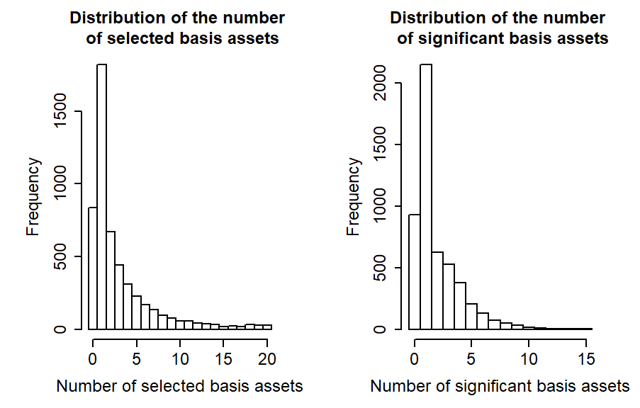
Figure 2.1: Distribution of the number of basis assets. The left figure shows the histogram of the number of basis assets selected by GIBS. On the right we report the histogram of number of basis assets significant in the second-step OLS regression at 5% level.

In addition, the results validate our sparsity assumption, that each company is significantly related to only a small number of basis assets (at a 5% level of significance). Indeed, for each company an average of 2.98 basis assets are selected by GIBS and an average of 1.92 basis assets show significance in the second stage OLS regression. (Even using the traditional cross-validation method with overfitting discussed in Section 2.6, only an average of 15.66 basis assets are selected.) In other words, the average number of elements in $S_{i}$ (see Equation 2.20) is 2.98 and the average number of elements in $S_{i}$ (see Equation 2.22) is 1.92. Figure 2.1 shows the distribution of the number of basis assets selected by GIBS and the number of basis assets that are significant in the second stage OLS regression. As depicted, most securities have between $1\sim 15$ significant basis assets. Thus high dimensional methods are appropriate and necessary here.

Table 2.2 provides the matrix $\bm{G}$ in percentage. Each grid is $100\cdot g_{b,d}$ where $g_{b,d}$ is defined in equation (2.25). Figure 2.2 is a heat map from which we can visualize patterns in Table 2.2. The darker the grid, the larger the percentage of significant basis assets. As indicated, different security classes depend on different classes of basis assets, although some basis assets seem to be shared in common. Not all of the Fama-French 5 risk-factors are significant in presence of the additional basis assets in our model. Only the market portfolio shows a strong significance for nearly all securities. The emerging market equities and the money market ETF basis assets seem to affect many securities as well. As shown, all of the basis assets are needed to explain security returns and different securities are related to a small number of different basis assets.

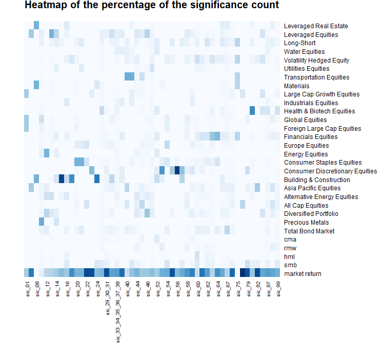
Figure 2.2: Heat map of percentage of significance count. Each grid are related to the percentage of basis assets selected in the corresponding sector (shown as the row name) by the company group (classified by the SIC code shown as the column name). The figure shows that different company groups may choose some basis assets in common, but also tends to select different sectors of basis assets.

ETF Class SIC First 2 digits 01 07 08 10 12 13 14 15 16 17 20 21 22 23 24 25-28 29-31 market return 25 50 0 7 20 21 25 30 26 44 32 33 62 62 30 33 62 smb 0 0 0 1 0 1 0 0 9 0 0 0 0 0 10 8 6 hml 0 0 0 1 0 1 0 0 4 0 1 0 0 0 0 1 2 rmw 0 0 0 0 0 0 0 0 0 0 0 0 0 0 0 3 0 cma 0 0 0 0 0 1 0 0 0 0 0 0 0 0 0 1 2 Total Bond Market 0 0 0 4 7 0 0 0 4 0 3 8 0 0 0 2 3 Precious Metals 0 0 0 36 0 0 12 0 0 0 0 0 0 0 0 1 0 Diversified Portfolio 0 0 0 2 20 9 6 0 0 0 1 0 0 0 0 1 2 All Cap Equities 0 0 0 1 0 0 0 0 0 0 3 0 12 0 0 2 0 Alternative Energy Equities 0 0 0 3 13 14 0 3 9 0 2 0 0 0 0 2 0 Asia Pacific Equities 0 25 0 3 7 0 0 0 0 0 1 0 0 0 0 1 3 Building & Construction 0 0 33 0 0 1 12 63 17 44 0 0 0 0 50 2 3 Consumer Discrtnry. Equities 0 0 0 0 0 0 0 0 0 0 2 0 0 31 0 0 6 Consumer Staples Equities 0 0 0 0 0 0 0 0 0 0 33 33 12 0 0 3 2 Energy Equities 0 0 0 6 33 1 6 0 0 0 0 0 0 0 0 0 0 Europe Equities 0 0 0 2 0 2 0 0 0 0 6 8 12 0 0 2 3 Financials Equities 0 0 0 1 0 1 6 0 4 0 0 0 0 0 0 2 2 Foreign Large Cap Equities 25 0 0 4 0 1 0 0 0 0 4 0 0 0 0 1 0 Global Equities 25 0 0 14 0 2 0 0 0 0 2 0 0 0 0 1 0 Health & Biotech Equities 0 0 0 1 0 0 0 0 0 0 0 0 0 0 0 17 2 Industrials Equities 0 0 0 0 0 1 0 0 9 0 0 0 0 0 0 1 0 Large Cap Growth Equities 25 0 0 0 0 1 0 0 0 0 1 0 0 8 0 2 0 Materials 0 0 33 2 0 2 0 0 0 0 1 0 0 0 10 2 0 Transportation Equities 0 0 0 1 0 0 0 0 0 0 0 0 0 0 0 1 0 Utilities Equities 0 0 0 0 0 1 6 0 0 0 0 8 0 0 0 2 0 Volatility Hedged Equity 0 0 0 1 0 1 0 0 4 11 4 0 0 0 0 1 0 Water Equities 0 0 0 0 0 0 0 0 0 0 1 0 0 0 0 1 0 Long-Short 0 0 0 4 0 4 6 3 0 0 4 8 0 0 0 4 0 Leveraged Equities 0 25 0 7 0 33 19 0 4 0 0 0 0 0 0 5 5 Leveraged Real Estate 0 0 33 0 0 0 0 0 9 0 0 0 0 0 0 0 0

Table 2.2: Table for the percentage of significance count. The table provides the matrix $\bm{G}$ in percentage (each grid is $100\cdot g_{b,d}$ where $g_{b,d}$ is defined in equation (2.25)). Each grid is the percentage of the basis asset selected in the corresponding sector (shown as the row name) by the company group (classified by the SIC code shown as the column name). Note that the elements in each column add up to 100, which means 100% (maybe be slightly different from 100 due to the rounding issue). The percent signs are omitted to save space.

ETF Class SIC First 2 digits 32 33-38 39 40 42 44 45 46 47-51 52 53 54 55 56 57 58 59 market return 38 40 54 15 28 33 26 27 30 25 34 35 60 30 36 42 48 smb 0 4 0 0 9 4 2 0 2 0 0 12 0 0 7 0 2 hml 0 1 0 0 0 0 0 0 0 0 0 0 0 0 0 0 0 rmw 0 0 0 0 0 4 0 0 1 0 7 0 0 0 0 4 0 cma 0 2 0 0 0 0 4 0 0 8 0 0 0 0 0 0 2 Total Bond Market 5 2 0 5 3 2 0 0 1 0 0 6 0 0 0 2 0 Precious Metals 0 0 0 0 0 0 0 0 1 0 0 0 0 0 0 0 0 Diversified Portfolio 5 0 0 0 0 10 4 27 7 0 0 0 4 0 0 2 7 All Cap Equities 0 2 0 10 0 6 19 2 4 0 0 0 0 0 0 6 0 Alternative Energy Equities 0 4 0 0 0 10 4 8 5 0 0 0 0 0 0 4 0 Asia Pacific Equities 5 2 0 20 0 2 6 2 1 0 0 0 0 0 0 0 4 Building & Construction 19 3 8 0 0 0 0 0 2 17 7 0 0 0 21 0 0 Consumer Discrtnry. Equities 0 2 8 0 0 0 0 0 1 8 41 0 24 67 29 6 11 Consumer Staples Equities 0 1 0 0 3 0 2 0 3 0 7 12 0 3 0 2 2 Energy Equities 0 2 0 0 0 4 2 2 0 8 0 0 0 0 0 0 0 Europe Equities 5 1 0 0 0 0 4 2 3 0 0 18 0 0 0 0 4 Financials Equities 0 1 8 0 0 0 0 2 1 8 0 0 0 0 0 4 0 Foreign Large Cap Equities 0 1 0 0 0 0 0 0 2 0 0 6 0 0 0 4 0 Global Equities 5 1 0 0 0 0 0 2 2 0 0 6 0 0 0 6 2 Health & Biotech Equities 0 5 0 0 0 0 2 0 2 8 0 0 0 0 0 0 0 Industrials Equities 0 3 8 0 6 0 0 0 2 0 0 0 0 0 0 0 7 Large Cap Growth Equities 0 1 0 0 6 2 2 0 1 0 0 0 0 0 0 0 4 Materials 0 0 0 0 0 2 2 0 1 0 3 0 0 0 0 0 0 Transportation Equities 0 0 0 35 34 2 15 0 1 0 0 0 0 0 0 0 0 Utilities Equities 0 0 0 0 0 2 0 2 12 0 0 0 0 0 0 0 0 Volatility Hedged Equity 0 2 0 5 3 6 0 0 4 0 0 6 4 0 0 6 2 Water Equities 0 6 8 5 3 0 0 0 2 8 0 0 0 0 0 0 0 Long-Short 5 5 0 5 0 4 0 2 3 8 0 0 8 0 7 4 0 Leveraged Equities 14 7 8 0 0 10 8 21 4 0 0 0 0 0 0 8 4 Leveraged Real Estate 0 0 0 0 3 0 0 0 2 0 0 0 0 0 0 0 0

Table 2.2 continued.

ETF Class SIC First 2 digits 60 61 62 63 64 65 67 70-73 75 78 79 80 82 83 87 89 99 market return 16 51 40 22 44 36 21 55 0 70 60 27 62 38 40 38 34 smb 10 0 4 5 0 2 2 4 0 0 15 5 6 0 5 0 8 hml 14 0 4 3 0 0 1 0 0 0 0 0 0 0 1 0 1 rmw 3 0 3 1 0 0 1 1 0 0 0 0 0 0 2 6 4 cma 0 0 0 0 0 0 0 0 0 0 0 0 0 0 1 0 1 Total Bond Market 5 5 5 0 6 2 19 3 0 0 0 0 0 0 4 0 3 Precious Metals 0 0 1 1 0 0 2 0 0 0 0 0 0 0 2 0 1 Diversified Portfolio 2 5 3 1 0 4 4 1 0 0 0 0 0 12 1 6 2 All Cap Equities 1 0 0 1 0 2 1 4 0 20 0 0 0 0 3 12 4 Alternative Energy Equities 2 2 2 1 0 0 2 3 0 0 0 3 0 0 1 0 3 Asia Pacific Equities 2 5 1 1 0 5 6 6 0 0 5 3 25 0 4 12 3 Building & Construction 0 0 0 0 0 7 1 1 0 0 0 0 0 0 2 0 1 Consumer Discrtnry. Equities 1 5 1 1 0 0 1 1 0 0 15 2 0 0 0 0 1 Consumer Staples Equities 3 2 6 5 12 0 1 1 0 0 0 2 0 0 2 0 1 Energy Equities 0 0 1 0 0 0 0 0 0 0 0 0 0 0 0 0 1 Europe Equities 2 2 1 4 0 2 2 2 0 0 0 0 0 0 0 0 1 Financials Equities 7 12 11 27 31 7 6 2 20 0 0 2 0 0 3 6 4 Foreign Large Cap Equities 2 0 0 1 0 0 2 1 0 0 0 0 0 0 2 0 1 Global Equities 2 0 2 1 0 2 2 1 0 0 5 0 0 0 1 6 1 Health & Biotech Equities 1 0 0 4 0 4 1 1 0 0 0 45 0 12 11 0 13 Industrials Equities 0 0 0 1 0 0 1 0 0 0 0 0 0 0 3 0 0 Large Cap Growth Equities 0 0 0 0 0 2 1 4 0 10 0 0 0 12 0 0 3 Materials 0 0 1 0 0 2 1 0 20 0 0 0 0 0 0 0 1 Transportation Equities 0 0 0 0 0 0 0 1 20 0 0 0 0 0 0 0 1 Utilities Equities 3 2 1 1 0 0 3 0 0 0 0 0 0 0 0 0 1 Volatility Hedged Equity 15 7 3 11 6 5 3 2 20 0 0 3 6 12 2 0 2 Water Equities 1 0 0 0 0 0 1 0 0 0 0 0 0 0 4 0 1 Long-Short 5 0 12 4 0 9 5 3 20 0 0 5 0 0 4 6 3 Leveraged Equities 2 0 1 1 0 4 2 1 0 0 0 0 0 12 1 0 1 Leveraged Real Estate 1 0 1 0 0 7 7 1 0 0 0 3 0 0 0 6 1

Table 2.2 continued.

2.5.1 Intercept Test

This section provides the tests for a zero intercept. Using the Fama-French 5-factor model as a comparison, Figure 2.3 compares the intercept test p-values between our basis asset implied Adaptive Multi-factor (AMF) model and Fama-French 5-factor (FF5) model. As indicated, 6.22% (above 5%) of the securities have significant intercepts in the FF5 model, while 3.86% (below 5%) of the securities in AMF have significant $\alpha$’s. This may suggests that the AMF model is more insightful than the FF5 model, since AMF reveals more relevant factors and makes the intercept closer to 0.

Since we replicate this test for about 5000 stocks in the CRSP database, it is important to control for a False Discovery Rate (FDR) because even if there is a zero intercept, a replication of 5000 tests will have about 5% showing false significance. We adjust for the false discovery rate using the Benjamini-Hochberg (BH) procedure [7] and the Benjamini-Hochberg-Yekutieli (BHY) procedures [8]. The BH method does not account for the correlation between tests, while the BHY method does. In our case, each test is done on an individual stock, which may have correlations. So the BHY method is more appropriate here.

Chordia et al. (2017) [15] suggests that the false discovery proportion (FDP) approach in [53] should be applied rather than a false discovery rate procedure. The BH approach only controls the expected value of FDP while FDP controls the family-wise error rate directly. There is another test worth mentioning, which is the GRS test. The GRS test in [24] is usually an excellent procedure for testing intercepts. However, these two tests are not appropriate in the high-dimensional regression setting as in our case. To be specific, these tests are implicitly based on the assumption that all companies are only related to the same small set of basis assets. Here the “small” means there are many fewer basis assets than observations. Our setting is more general since we may have more basis assets than observations, although each company is related to only a small number of basis assets, different companies may be related to different sets of basis assets. The GRS is unable to handle setting.

As noted earlier, Table 2.3 shows that 3.86% of stocks in the multi-factor model have p-values for the intercept t-test of less than 0.05. While in the FF5 model, this percentage is 6.22%. After using the BHY method to control for the false discovery rate, we can see that the q-values (the minimum false discovery rate needed to accept that this rejection is a true discovery, see [57]) for both models are almost 1, indicating that there are no significant non-zero intercepts. All the significance shown in the intercept tests is likely to be false discovery. This is the evidence that both models are consistent with the behavior of “large-time scale” security returns.

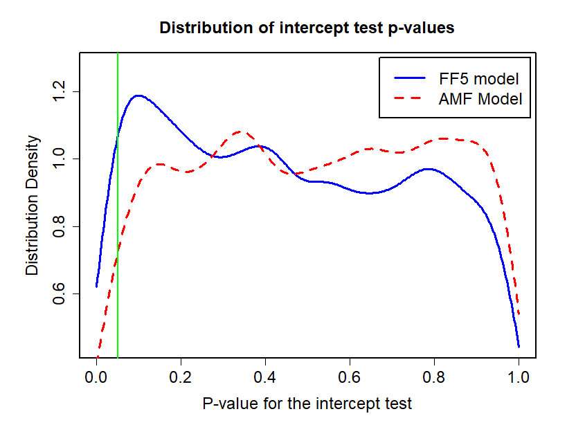
Figure 2.3: Comparison of intercept test p-values for the Fama-French 5-factor (FF5) model and the Adaptive Multi-factor (AMF) model.

Value Range	Percentage of Stocks (%)
	FF5 p-val	AMF p-val	FF5 FDR q-val	AMF FDR q-val
0 - 0.05	6.22	3.86	0.00	0.00
0.05 - 0.9	84.88	85.33	0.02	0.00
0.9 - 1	8.90	10.81	99.98	100.00

Table 2.3: Intercept Test with control of false discovery rate. The first column is the value range of p-values or q-values listed in the other columns. The other 4 columns are related to p-values and False Discovery Rate (FDR) q-values for the FF5 model and the AMF model. For each column, we listed the percentage of companies with values within each value range. It is clear that nearly all rejections of zero-alpha are false discoveries.

2.5.2 In-Sample and Out-of-Sample Goodness-of-Fit

This section tests to see which model fits the data best. Figure 2.4 compares the distribution of the adjusted $R^{2}$’s (see [58]) between the AMF and the FF5 model. As indicated, the AMF model has more explanatory power. The mean adjusted $R^{2}$ for the AMF model is 0.319 while that for the FF5 model is 0.229. The AMF model increases the adjusted $R^{2}$ by 39.2% compared to the FF5.

We next perform an F-test, for each security, to show that there is a significant difference between the goodness-of-fit of the AMF and the FF5 model. Since we need a nested comparison for an F-test, we compare the results between FF5 and GIBS + FF5 (which is including FF5 factors back to GIBS for fitting if any of the FF5 factors are not selected). In our case, the FF5 is the restricted model, having $p-r_{1}$ degrees of freedom and a sum of squared residuals $SS_{R}$, where $r_{1}=5$. The AMF is the full model, having $p-r_{1}-r_{2}$ degrees of freedom (where $r_{2}$ is the number of basis assets selected in addition to FF5) and a sum of squared residuals $SS_{F}$. Under the null-hypothesis that FF5 is the true model, we have

$$F_{obs}=\frac{(SS_{R}-SS_{F})/r_{2}}{SS_{F}/(p-r_{1}-r_{2})}\overset{H_{0}}{\sim}F_{r_{2},p-r_{1}-r_{2}}.$$ (2.26)

There are 5132 stocks in total. For 1931 (37.63%) of them, the GIBS algorithm only selects some of the FF5 factors, so for these stocks, GIBS + FF5 does not give extra information. However, for 3201 (62.37%) of them, the GIBS algorithm does select ETFs outside of the FF5 factors. For these stocks, we do the F test to check whether the difference between the two models are significant, in other words, whether AMF gives a significantly better fit. As shown in Table 2.4, for 97.72% of the stocks, the AMF model fits better than the FF5 model.

Again, it is important to test the False Discovery Rate (FDR). Table 2.4 contains the p-values and the false discovery rate q-values using both the BH method and BHY methods. As indicated, for most of the stocks, the AMF is significantly better than the FF5 model, even after considering the false discovery rate. For 97.72% of stocks, the AMF model is better than the FF5 at the significance level of 0.05. After considering the false discovery rate using the strict BHY method which includes the correlation between tests, there is still 90.16% of stocks significant with q-values less than 0.05. Even if we adjust our false discover rate q-value significance level to 0.01, there is still 83.29% of the stocks showing a significant difference. As such, this is strong evidence supporting the multi-factor model’s superior performance in characterizing security returns.

Figure 2.4: Comparison of adjusted $R^{2}$ for the Fama-French 5-factor (FF5) model and the Adaptive Multi-factor (AMF) model

Value Range	Percentage of Stocks
	p-value	BH q-value	BHY q-value
$0\sim 0.01$	93.44%	93.06%	83.29%
$0\sim 0.05$ (Significant)	97.72%	97.53%	90.16%
$0.05\sim 1$ (Non-Significant)	2.28%	2.47%	9.84%

Table 2.4: F test with control of false discovery rate. We do the F test and report its p-value, q-values for each company. The first column is the value range of p-values or q-values listed in the other columns. In the other three columns we report percentage of companies with p-value, BH method q-value, and BHY method q-value in each value range. The table shows that for most companies the increment of goodness of fit is very significant.

Apart from the In-Sample goodness of fit results, we also compare the Out-of-Sample goodness of fit of the FF5 and AMF model in the prediction time period. We use the two models to predict the return of the following week and report the Out-of-Sample $R^{2}$ for the prediction (see Table 2.5). The Out-of-Sample $R^{2}$ (see [14]) is used to measure the predictive accuracy of a model. The Out-of-Sample $R^{2}$ for the FF5 is $0.030$, while that for the AMF is $0.038$. That is, the AMF model increased the Out-of-Sample $R^{2}$ by $24.07\%$ compared to the FF5 model. The AMF model shows its superior performance by giving a more accurate prediction using an even lower number of factors, which is also strong evidence against overfitting. The AMF model provides additional insight when compared to the FF5.

2.5.3 Robustness Test

As a robustness test, for those securities whose intercepts were non-zero, we tested the basis asset implied multi-factor model to see if positive alpha trading strategies generate arbitrage opportunities. To construct the positive alpha trading strategies, we use the data from the year 2017 as an out-of-sample period. Recall that the previous analysis was over the time period 2014 to 2016. As explained above, we fit the AMF model using the data up to the last week of 2016. We then ranked the securities by their alphas from positive to negative. We take the top 50% of those with significant (p-val less than 0.05) positive alphas and form a long-only equal-weighted portfolio with $1 in initial capital. Similarly, take the bottom 50% of those with significant negative alphas and form a short-only equal-weighted portfolio with -$1 initial capital. Then, each week over 2017, we update the two portfolios by re-fitting the AMF model and repeating the same construction. Combining the long-only and short-only portfolio forms a portfolio with 0 initial investment. If the alphas represent arbitrage opportunities, then the combined long and short portfolio’s change in value will always be non-negative and strictly positive for some time periods.

The results of the arbitrage tests are shown in Figures 2.5 and 2.6. As indicated, the change in value of the 0-investment portfolio randomly fluctuates on both sides of 0. This rejects the possibility that the positive alpha trading strategy is an arbitrage opportunity. Thus, this robustness test confirms our previous intercept test results, after controlling for a false discovery rate. Although not reported, we also studied different quantiles from 10% to 40% and they give similar results.

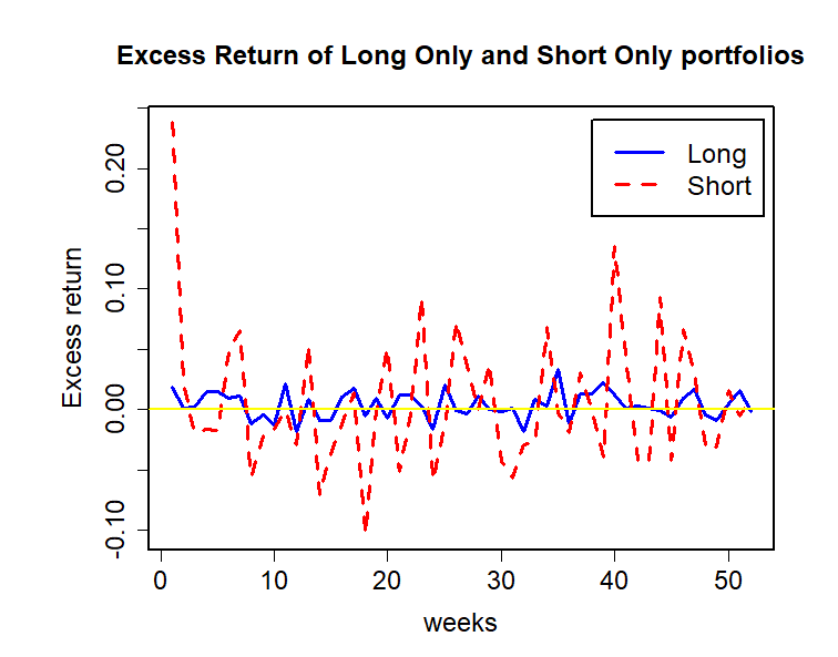
Figure 2.5: Returns of Long-only and Short-only Portfolio

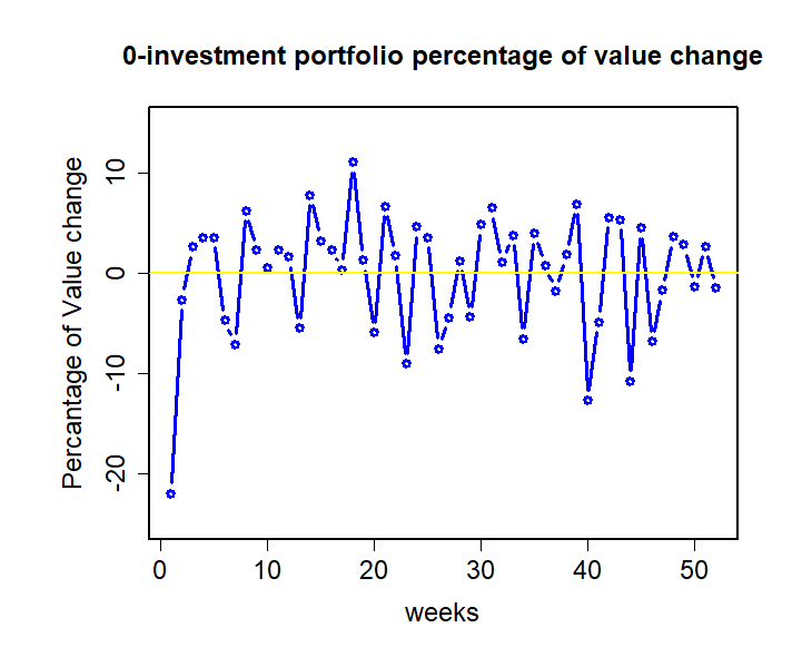
Figure 2.6: Percentage of Value Change of 0-Investment portfolio

2.6 Comparison with Alternative Methods

2.6.1 Are Fama-French 5 Factors Overfitting?

We first test whether the Fama-French 5 factors (FF5) overfit the noise in the data. This can be done by estimating a “GIBS + FF5” model. This model is very similar to GIBS, except that it includes the Fama-French 5 factors to be selected in the last step. That is, if any of the FF5 factors are not selected by GIBS, we add them back to our selected basis asset set $\widetilde{S}_{i}$ and use this set of basis assets to fit and predict the returns. By comparing the In-Sample Adjusted $R^{2}$ and the Out-of-Sample $R^{2}$ (see [14]) of GIBS + FF5 model and the GIBS model, we can determine whether FF5 factors are overfitting. The Out-of-Sample $R^{2}$ (see [14]) is used to measure the accuracy of prediction of a model. Surprisingly, the results show that some of the FF5 factors are over-fitting! As shown in Table 2.5, compared to our GIBS model, the GIBS + FF5 achieves a better in-sample Adjusted $R^{2}$, with more significant basis assets, but gives a much worse Out-of-Sample $R^{2}$. This indicates that the FF5 factors not selected by GIBS are “false discoveries” - they overfit the training data, but do a poor job in predicting. Therefore, those FF5 factors should not be used for a company if they are not selected by GIBS. Table 2.5 not only provides evidence of the superior performance of GIBS over FF5 by comparing the In-Sample Adjusted $R^{2}$ and Out-of-Sample $R^{2}$ of GIBS and FF5 model, but it also indicates an overfitting of FF5 by comparing the In-Sample Adjusted $R^{2}$ and Out-of-Sample $R^{2}$ of GIBS and GIBS + FF5.

2.6.2 Comparison with Elastic Net

Since there are a large number of correlated ETFs it is natural to employ the RIDGE, LASSO and Elastic Net (E-Net) methods (by Zou and Hastie (2005) [73]). E-Net is akin to the ridge regression’s treatment of multicollinearity with an additional tuning (ridge) parameter, $\alpha$, that regularizes the correlations. We compare GIBS, LASSO, RIDGE and E-Net with different $\alpha$s. The sparsity inducing parameter $\lambda$ in each model is selected by the usual 10-fold cross-validation (by Kohavi et al. (1995) [43]). The comparison results are shown in Table 2.5. The distribution of the number of basis assets selected by each method is shown in Figure 2.7.

From Table 2.5 it is clear that the GIBS model has better prediction than the FF5 model. The GIBS model increased the Out-of-Sample $R^{2}$ by 24.07% compared to FF5. Across all models, GIBS has the highest Out-of-Sample $R^{2}$, which supports the fact that the better In-Sample Adjusted $R^{2}$ achieved by the other models (LASSO, RIDGE, E-Net etc.) is due to overfitting. Furthermore, from Table 2.5 and Figure 2.7, we see that GIBS selects the least number of factors.

Model Select Signif. In-Sample Adj. $R^{2}$ Out-of-Sample $R^{2}$ FF5 5.00 1.78 0.229 (00.00%) 0.030 (00.00%) GIBS 2.98 1.92 0.319 (39.18%) 0.038 (+24.07%) GIBS + FF5 7.20 2.50 0.350 (52.55%) 0.025 (-16.71%) LASSO 15.66 5.72 0.466 (103.46%) 0.018 (-40.97%) E-Net ($\alpha$=0.75) 16.84 5.81 0.470 (105.22%) 0.018 (-40.09%) E-Net ($\alpha$=0.50) 19.28 6.05 0.479 (109.05%) 0.015 (-49.92%) E-Net ($\alpha$=0.25) 26.36 6.51 0.498 (117.20%) 0.009 (-70.33%) Ridge 182.00 NA NA -6$\times 10^{4}$ (-2$\times 10^{8}$%)

Table 2.5: Comparison table for Alternative Methods. The “Select” column gives the average count of the factors selected by the model. The “Signif.” column gives the average count of the significant factors selected by the model. The column “In-sample Adj. $R^{2}$” gives the average in-sample Adjusted $R^{2}$ for each model, the percentage in the bracket is the percentage change compared to the FF5 model. The column “Out-of-Sample $R^{2}$” gives the average Out-of-Sample $R^{2}$ for each model, the percentage in the bracket is the percentage change compared to the FF5 model.

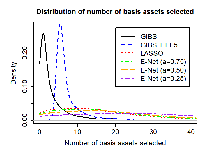
Figure 2.7: Comparison of number of basis assets selected by cross-validation for different methods.

The $\lambda$ of LASSO is traditionally selected by cross-validation and with this $\lambda$, the model selects an average of 15.66 factors, as shown in Table 2.5. However, most of the factors selected by cross-validation are “false-positive”. Therefore, instead of the cross-validation, we use the “1se rule” with a hard threshold 20 basis assets at most. The “1se rule” use the largest $\lambda$ such that the cross-validation error is within one standard error of the minimum error achieved by the cross-validation. In another word, $\lambda_{1se}$ gives the most regularized model such that error is within one standard error of the minimum error achieved by the cross-validation (see [23, 56, 60]). To further avoid over-fitting, we include the threshold that each company can not be related to more than 20 basis assets. As shown in the Table 2.5, our method used in GIBS works well and achieves the best prediction power. The reason for the superior performance of GIBS compared with the cross-validation LASSO is that cross-validation often overfits, especially when the sample size is small, or when the data is not sufficiently independent and identically distributed. In addition, our results with GIBS are both stable and interpretable.

Our choice of dimension reduction techniques, using a combination of prototype clustering and a modified version of LASSO, was motivated by our desire to select, from a collection of strongly correlated ETFs, a sparse and interpretable set of basis assets that explains the cross-sectional variation among asset returns. These two steps were used as model selection tools to identify basis assets, and we subsequently estimated the model coefficients using OLS. In future research, a more integrative method may be designed to combine the model selection and estimation steps.

The motivation for using prototype clustering is two fold. First, it can be used to derive the cluster structure of the ETFs so that the redundant ones are removed. This reduces the correlation and validates the use of LASSO. Second, this method gives a clear interpretation of the prototypes, which is important for our interpretation of the basis assets. The traditional methods of dealing with empirical asset models are based on variance decomposition of the basis assets (the $X$ matrix) as in, for example, the principal component analysis (PCA) approach. More recently, there are modern statistical methods that introduce sparsity and high-dimensional settings in these traditional methods (see Zou et al. (2006) [74]). However, as we argued in the introduction, these methods are not optimal for basis asset models due to their difficulties in interpreting the basis assets. Furthermore, it is the correlation that is important in the determination of the basis assets not the variance itself. Therefore, methods that focus on finding the rotation with the largest variance (like PCA) are not optimal in this setting. Instead, we use correlation as our metric in the prototype clustering step, which gives a clearer interpretation and a direct analysis of the candidate basis assets, rather than linear combinations of the basis assets. For this reason we believe that prototype clustering is preferred to PCA in this setting.

For future work, modern refinements of model-selection and inference methods may be used. For high-dimensional models obtaining valid p-values is difficult. This is in part due to the fact that fitting a high-dimensional model often requires penalization and complex estimation procedures, which implies that characterizing the distribution of such estimators is difficult. For statistical testing in the presence of sparsity a number of new methods are appearing in the literature. One alternative method is the post-selection procedure by Tibshirani et al. (2016) [61]. Another approach for constructing frequentistp p-values and confidence intervals for high-dimensional models uses the idea of de-biasing which was proposed in a series of articles [62, 38, 65]. In the de-biasing method, starting from a regularized estimator one first constructs a de-biased estimator and then makes inference based on the asymptotic normality of low-dimensional functionals of the de-biased estimator. In principle, this approach also provides asymptotically valid p-values for hypotheses testing each of the parameters in the model. However, in our numerical explorations of these methods we found that the confidence intervals are too large for the current application and no meaningful insights could be obtained. The p-values for these methods are also not very stable. So we use the OLS after LASSO instead of the post-selection methods with the theoretical guarantee in the paper by Zhao et al. (2017) [67]. Some details can be found in [69]. Some related work can be found in [70, 71, 72, 37, 46, 12, 64, 32, 30, 29, 31, 48, 66, 17, 51, 68, 40, 47, 41, 39].

2.7 Risk-Factor Determination

We focus on the same three year time period 2014 - 2016 and compute the average annal excess returns on the basis assets to determine which have non-zero risk premium (average excess returns), i.e. which are risk-factors in the traditional sense. In this time period there are 182 basis assets selected, including the Fama-French 5 factors and 177 ETFs. The risk premium of the Fama-French 5 factors are shown in Table 2.6.

Fama-French 5 Factors	Market Return	SMB	HML	RMW	CMA
Annual Excess Return (%)	10.0	-2.1	1.7	1.1	-1.2

Table 2.6: Risk Premium of Fama-French 5 factors

Out of the 177 selected ETFs, 136 of them have absolute risk premiums larger than the minimum of that of the FF5 factors (which is the RMW, with absolute risk premium 1.1%). Therefore, at least $(136+5)/(177+5)=77.47\%$ basis assets are risk factors. Furthermore, 29 out of the 177 selected ETFs have absolute risk premiums larger than 10.0% (the absolute risk premium of the market return, which is the biggest absolute risk premium of all FF5 factors). The list of the 29 ETFs are in Table 2.7.

Risk Pre- ETF name Category mium (%) ProShares Ultra Semiconductors Leveraged Equities 55.1 ProShares Ultra Bloomberg Natural Gas Leveraged Commodities -30.4 ProShares VIX Short-Term Futures ETF Volatility -29.2 ProShares Ultra Real Estate Leveraged Real Estate 26.2 Global X MSCI Nigeria ETF Foreign Large Cap Equities -24.0 Invesco DB Oil Fund Oil & Gas -21.3 Global X FTSE Greece 20 ETF Emerging Markets Equities -20.8 Invesco S&P SmallCap Information Technology ETF Technology Equities 19.7 Direxion Daily Energy Bull 3X Shares Leveraged Equities -17.5 Invesco S&P SmallCap Consumer Staples ETF Consumer Staples Equities 15.8 VanEck Vectors Rare Earth/Strategic Metals ETF Materials -15.5 Global X Uranium ETF Global Equities -15.3 SPDR S&P Health Care Equipment ETF Health & Biotech Equities 15.0 SPDR SSGA US Small Cap Low Volatility Index ETF Volatility Hedged Equity 15.0 Vanguard Utilities ETF Utilities Equities 15.0 VanEck Vectors Egypt Index ETF Emerging Markets Equities -15.0 Global X MSCI Colombia ETF Latin America Equities -14.6 SPDR S&P Insurance ETF Financials Equities 14.2 iShares U.S. Aerospace & Defense ETF Industrials Equities 13.8 iShares North American Tech-Software ETF Technology Equities 13.4 iShares North American Tech-Multimedia Networking ETF Communications Equities 13.3 FLAG-Forensic Accounting Long-Short ETF Long-Short 12.2 SPDR SSGA US Large Cap Low Volatility Index ETF Volatility Hedged Equity 12.0 Global X MSCI Portugal ETF Europe Equities -11.7 Vanguard Consumer Staples ETF Consumer Staples Equities 10.9 VanEck Vectors Poland ETF Europe Equities -10.8 VanEck Vectors Morningstar Wide Moat ETF Large Cap Blend Equities 10.6 Invesco Russell Top 200 Equal Weight ETF Large Cap Growth Equities 10.2 First Trust NASDAQ CEA Smartphone Index Fund Technology Equities 10.1

Table 2.7: List of ETFs with large absolute risk premium.

2.8 Illustrations

In this section we illustrate our multi-factor estimation process and compare the results with the Fama-French 5-factor (FF5) model for three securities: Adobe, Bank of America, and Apple.

2.8.1 Adobe

This section contains the results for Adobe. Using Equation (2.14), we estimate the Fama-French 5 factor (FF5) model as shown in Table 2.8. For our Adaptive Multi-Factor (AMF) model, the final results are shown in Table 2.9 with the description of the ETF basis assets selected by GIBS in Table 2.10. The adjusted $R^{2}$ for FF5 is 0.38, while the adjusted $R^{2}$ for AMF is 0.57. From the Tables it is clear that different significant basis assets are selected and the ones selected by GIBS gives much better explanation and prediction power. Only the market return is significant among the FF5 factors. Additionally, Adobe’s returns are related to the iShares North American Tech-Software ETF, indicating that Adobe is sensitive to risks in the technology software sector. For Adobe, both models do not have a significant intercept, indicating that the securities are properly priced.

	$\beta$	SE	t value	P-value
(Intercept)	0.002	0.002	1.227	0.222
Market Return	1.036	0.124	8.382	0.000
SMB	-0.168	0.191	-0.883	0.379
HML	-0.480	0.247	-1.942	0.054
RMW	-0.378	0.310	-1.217	0.226
CMA	-0.234	0.424	-0.551	0.583

Table 2.8: Adobe with the FF5 model. The column $\beta$ provides the coefficients in the OLS regression of Adobe on FF5 factors. The standard error (SE), t value, and P-value related to each coefficient are also provided.

$\beta$ SE t value P-value (Intercept) 0.002 0.002 1.110 0.269 Market Return -0.518 0.194 -2.662 0.009 iShares North American Tech-Software ETF 1.377 0.150 9.162 0.000

Table 2.9: Adobe with the AMF. The column $\beta$ provides the coefficients in the second-step OLS regression of Adobe on basis assets selected in the AMF. The standard error (SE), t value, and P-value related to each coefficient are also provided.

ETF Name Category Big Class iShares North American Tech-Software ETF Technology Equities Equity

Table 2.10: Significant ETF basis assets for Adobe. This table shows the category and big class of each ETF basis asset selected in the AMF.

2.8.2 Bank of America

This section contains the results for the Bank of America (BOA). The results are found in Tables 2.11, 2.12, and 2.13. The adjusted $R^{2}$ for FF5 is 0.72 while the adjusted $R^{2}$ for AMF is 0.82. For BOA, it is related to all of the FF5 factors except SMB. It is related to VanEck Vectors Investment Grade Floating Rate ETF, FlexShares Ready Access Variable Income Fund, and the WisdomTree Barclays Negative Duration U.S. Aggregate Bond Fund, indicating that BOA’s security returns (as a bank) are subject to risks related to the term structure of interest rates and the credit risk embedded in corporate bonds. It is also related to the SPDR SSgA Multi-Asset Real Return ETF which is correlated to the health of the economy. Finally, the $\alpha$’s in both models are not significantly different from zero, indicating that no arbitrage opportunities exist for this security.

	$\beta$	SE	t value	P-value
(Intercept)	0.000	0.002	0.274	0.784
Market Return	1.042	0.098	10.580	0.000
SMB	0.236	0.152	1.552	0.123
HML	1.981	0.197	10.046	0.000
RMW	-1.145	0.247	-4.627	0.000
CMA	-2.059	0.338	-6.087	0.000

Table 2.11: BOA with the FF5 model. The column $\beta$ provides the coefficients in the OLS regression of BOA on FF5 factors. The standard error (SE), t value, and P-value related to each coefficient are also provided.

$\beta$ SE t value P-value (Intercept) 0.001 0.001 0.405 0.686 Market Return 2.314 0.316 7.335 0.000 HML 1.078 0.146 7.390 0.000 RMW -0.752 0.221 -3.398 0.001 VanEck Vectors Investment Grade Floating Rate ETF 3.347 0.871 3.842 0.000 ProShares Short 7-10 Year Treasury -0.359 0.318 -1.129 0.261 SPDR SSgA Multi-Asset Real Return ETF -0.712 0.218 -3.259 0.001 FlexShares Ready Access Variable Income Fund -3.421 1.710 -2.000 0.047 IQ Hedge Market Neutral Tracker ETF -0.773 0.513 -1.507 0.134 SPDR SSGA US Large Cap Low Volatility Index ETF -0.405 0.230 -1.758 0.081 AdvisorShares Newfleet Multi-Sector Income ETF -1.460 0.852 -1.714 0.089 WisdomTree Barclays Negative Duration U.S. Aggregate Bond Fund 0.451 0.220 2.047 0.043 Vanguard Consumer Staples ETF -0.290 0.181 -1.604 0.111 Vanguard Utilities ETF -0.118 0.099 -1.196 0.234 Invesco CurrencyShares Swiss Franc Trust -0.152 0.079 -1.925 0.056 iShares Short Treasury Bond ETF -13.968 8.592 -1.626 0.106 Invesco DB Precious Metals Fund -0.011 0.088 -0.121 0.904 SPDR Barclays Short Term Municipal Bond -0.011 0.927 -0.012 0.990 iShares Moderate Allocation ETF -0.087 0.600 -0.146 0.885 ProShares Ultra Yen -0.008 0.067 -0.123 0.902

Table 2.12: BOA with the AMF. The column $\beta$ provides the coefficients in the second-step OLS regression of BOA on basis assets selected in the AMF. The standard error (SE), t value, and P-value related to each coefficient are also provided.

ETF Name Category Big Class VanEck Vectors Investment Grade Floating Rate ETF Corporate Bonds Bond/Fixed Income SPDR SSgA Multi-Asset Real Return ETF Hedge Fund Alternative ETFs FlexShares Ready Access Variable Income Fund Corporate Bonds Bond/Fixed Income WisdomTree Barclays Negative Duration U.S. Aggregate Bond Fund Total Bond Market Bond/Fixed Income

Table 2.13: Significant ETF basis assets for BOA. This table shows the category and big class of each ETF basis asset selected in the AMF.

2.8.3 Apple

This section gives the results for Apple, in Tables 2.14, 2.15, pand 2.16. The adjusted $R^{2}$ for FF5 is 0.52, while the adjusted $R^{2}$ for our AMF model is 0.64. For Apple, the market return, RMW, CMA are the significant FF5 factors. It is significantly related to First Trust NASDAQ CEA Smartphone Index Fund, since Apple produces smartphones. The remaining ETFs capture the health of the equities and bond markets, documenting that Apple’s risk are highly correlated with the general economy as well. Finally, the $\alpha$’s in both models are not significantly different from zero.

	$\beta$	SE	t value	P-value
(Intercept)	0.000	0.002	0.208	0.836
Market Return	1.106	0.119	9.313	0.000
SMB	-0.334	0.183	-1.825	0.070
HML	0.359	0.238	1.511	0.133
RMW	1.242	0.298	4.163	0.000
CMA	-2.371	0.408	-5.811	0.000

Table 2.14: Apple with the FF5 model. The column $\beta$ provides the coefficients in the OLS regression of Apple on FF5 factors. The standard error (SE), t value, and P-value related to each coefficient are also provided.

$\beta$ SE t value P-value (Intercept) -0.002 0.002 -0.972 0.333 Market Return 2.062 0.380 5.430 0.000 SMB -0.092 0.184 -0.502 0.617 RMW 1.135 0.259 4.389 0.000 CMA -1.780 0.295 -6.043 0.000 First Trust NASDAQ CEA Smartphone Index Fund 0.327 0.157 2.079 0.039 iShares Floating Rate Bond ETF 6.831 2.412 2.832 0.005 AGFiQ US Market Neutral Momentum Fund -0.311 0.089 -3.485 0.001 Invesco Dynamic Media ETF -0.428 0.162 -2.636 0.009 Invesco Water Resources ETF -0.228 0.195 -1.167 0.245 VanEck Vectors Environmental Services ETF -0.389 0.206 -1.890 0.061 ProShares Ultra Semiconductors 0.014 0.060 0.233 0.816 iShares MSCI Israel ETF -0.615 0.128 -4.818 0.000

Table 2.15: Apple with AMF. The column $\beta$ provides the coefficients in the second-step OLS regression of Apple on basis assets selected in the AMF. The standard error (SE), t value, and P-value related to each coefficient are also provided.

ETF Name Category Big Class First Trust NASDAQ CEA Smartphone Index Fund Technology Equities Equity iShares Floating Rate Bond ETF Corporate Bonds Bond/Fixed Income AGFiQ US Market Neutral Momentum Fund Long-Short Alternative ETFs Invesco Dynamic Media ETF All Cap Equities Equity iShares MSCI Israel ETF Large Cap Blend Equities Equity

Table 2.16: Significant ETF pbasis assets for Apple. This table shows the category and big class of each ETF basis asset selected in the AMF.

2.9 Conclusion

Using a collection of basis assets, the purpose of this paper is to test the new Adaptive Multi-Factor (AMF) model implied by the generalized arbitrage pricing theory (APT) recently developed by Jarrow and Protter (2016) [35] and Jarrow (2016) [34]. The idea is to obtain the collection of all possible basis assets and to provide a simultaneous test, security by security, of which basis assets are significant. Since the collection of basis assets selected for investigation is large and highly correlated, we propose a new high-dimensional algorithm – the Groupwise Interpretable Basis Selection (GIBS) algorithm to do the analysis. For comparison with the existing literature, we compare the performance of AMF (using the GIBS algorithm) with the Fama-French 5-factor model and all other alternative methods. Both the Fama-French 5-factor and the AMF model are consistent with the behavior of “large-time scale” security returns. In a goodness-of-fit test comparing the AMF with Fama-French 5-factor model, the AMF model has a substantially larger In-Sample adjusted $R^{2}$ and Out-of-Sample $R^{2}$. This documents the AMF model’s superior performance in characterizing security returns. Last, as a robustness test, for those securities whose intercepts were non-zero (although insignificant), we tested the AMF model to see if positive alpha trading strategies generate arbitrage opportunities. They do not, thereby confirming that the multi-factor model provides a reasonable characterization of security returns.

Chapter 3 Time-Invariance Coefficients Tests with the Adaptive Multi-Factor Model

3.1 Introduction

The purpose of this paper is to test the multi-factor beta model implied by the generalized arbitrage pricing theory (APT) of Jarrow and Protter (2016) [35], and recently tested by Zhu et al. (2018) [69], without imposing the exogenous assumption of constant betas. The assumption of time-invariant beta coefficients in multi-factor models is an often employed one in the empirical literature, see Jagannathan et al. (2010) [33] and Harvey et al. (2016) [25] for reviews. In the paper by Zhu et al. (2018) [69], they address the restrictive nature of this assumption by estimating the model over a short time horizon - three years. For many applications, restricting the time horizon to such a short time period is problematic. Alternative approaches for fitting time-varying betas over longer time horizons have been proposed and estimated, such as the conditional factor models. See paper Adrian et al. (2015) [1], Cooper & Maio (2019) [16], and Avramov & Chordia (2006) [4]. In contrast to these approaches, we show herein that this constant beta assumption can be avoided if we use the Adaptive Multi-Factor (AMF) model with the Groupwise Interpretable Basis Selection (GIBS) algorithm in a dynamic manner using a comparably short rolling window. This insight is a direct corollary of the generalized APT.

Using the Adaptive Multi-Factor (AMF) model with the Groupwise Interpretable Basis Selection (GIBS) algorithm proposed in Zhu et al. (2018) [69], but fitting price differences instead of returns, we estimated a multi-factor model to stock prices over the time period 2007 - 2018. Employing the collection of Exchange Traded Funds (ETFs) as potential factors, we use the high dimensional GIBS algorithm to select the factors for each company. No-arbitrage tests confirm the validity of the generalized APT. As a robustness check, we also show that the estimated model performs better than the traditional Fama-French 5-factor model. After this validation, we perform the time-invariance tests for the $\beta$ coefficients for various time periods. At last, we found that for time periods no more than 5 years, the beta coefficients are time-invariant for the AMF model. Using a dynamic AMF model with a rolling window with a length of no more than 5 years gives a good fit. The arbitrage test confirms the validity of generalized APT’s theory.

An outline for this paper is as follows. Section 3.2 presents the Generalized APT theory. Section 3.3 provides the estimation methodology. Section 3.4 provides the testing methodology and results. Section 3.5 concludes.

3.2 The Generalized APT

Jarrow and Protter (2016) derive a testable multi-factor model over a finite horizon [0, T] in the context of a continuous time, continuous trading market assuming only frictionless and competitive markets that satisfy no-arbitrage and no dominance, i. e. the existence of an equivalent martingale measure. As in the traditional asset pricing models, adding a non-zero alpha to this relation (Jensen’s alpha) implies a violation of the no-arbitrage condition.

The generalized APT uses linear algebra to prove the existence of an algebraic basis in the security’s payoff space at some future time T. Since this is is a continuous time and trading economy, this payoff space is infinite-dimensional. The algebraic basis at time T constitutes the collection of tradeable basis assets and it provides the multi-factor model for a security’s price at time T. The coefficients of the time T multi-factor model are constants (non-random). No-arbitrage, the existence of the martingale measure, implies that the arbitrage-free prices of the risky assets at all earlier dates $t\in[0,T)$ will satisfy the same factor model and with the same constant coefficients. Transforming prices into returns (dividing prices at time $t+1$ by time $t$ prices to get the return at $t+1$), makes the resulting coefficients in the multi-factor model stochastic when viewed at time $0$. However, this is not the case for the multi-factor model specified in a security’s price (or price differences). The multi-factor model’s beta coefficients in the security’s price process are time-invariant.

The generalized APT is important for practice because it provides an exact identification of the relevant set of basis assets characterizing a security’s realized (emphasis added) returns. This enables a more accurate risk-return decomposition facilitating its use in trading (identifying mispriced assets) and for risk management. Taking expectations of this realized return relation with respect to the martingale measure determines which basis assets are risk-factors, i.e. which basis assets have non-zero expected excess returns (risk premiums) and represent a systematic risk. Since the traditional models are nested within the generalized APT, an empirical test of the generalized APT provides an alternative method for testing the traditional models as well.

Let $B(t)$ denote the time $t$value of a money market account (mma) with initial value of 1 dollar at time 0, i.e.

$$B(t)=1\cdot\prod_{k=0}^{t-1}\Big{[}1+r_{0}(k)\Big{]}$$ (3.1)

where $r_{0}(k)$ is the default-free spot rate (the risk-free rate) from time $k$ to time $k+1$.

Let $A_{i}(t)$ denote the market price of the $i^{th}$ stock at time $t$ for $i=1,\ldots,N_{c}$. To include cumulative cash flows and stock splits into the valuation methodology, we need to compute the adjusted price $Y_{i}$, which is reconstructed by the using the security’s returns, after being adjusted for dividends and stock splits:

$$Y_{i}(t)=A_{i}(0)\prod_{k=0}^{t-1}\Big{[}1+R_{i}(k)\Big{]}$$ (3.2)

where $A_{i}(0)$ is the initial price and $R_{i}(k)$ its return over $[k,k+1]$.

Let $V_{j}(t)$ be the adjusted price of the $j^{th}$ basis asset at time $t$ for $j=1,\ldots,N_{f}$. Here, the sources of the basis asset in our model are the Fama-French 5 factors and the Exchange-Traded Funds (ETF). We include within this set of risk-factors the MMA. For notational simplicity, we let $V_{1}(t)=B(t)$.

Given this notation, the generalized APT implies the following multi-factor model for the $i^{th}$ security’s time $t$ price:

$$Y_{i}(t)=\sum_{j=1}^{N_{f}}\beta_{i,j}V_{j}(t)+\epsilon_{i}(t)$$ (3.3)

where $\beta_{i,j}$ for all $i,j$ are constants and $\tilde{\epsilon}_{i}(t)$ is an i.i.d. error term with zero mean and constant variance.

The goal of our estimation is two-fold. First, we want to test to see whether expression (3.3) provides a good fit to historical stock price data. Second, we want to investigate whether the multi-factors coefficients $\beta_{i,j}$’s are time-invariant. Given that prices are known to be autocorrelated, instead of estimating expression (3.3), we fit the first order price differences of this expression:

$$\Delta Y_{i}(t)=Y_{i}(t+1)-Y_{i}(t)=\sum_{j=1}^{N_{f}}\beta_{i,j}\Delta V_{j}(t)+\Delta\epsilon_{i}(t)$$ (3.4)

where $\Delta\epsilon_{i}(t)=\epsilon_{i}(t+1)-\epsilon_{i}(t)$.

For a given time period $(t,T)$, letting $n=T-t+1$, $p=N_{f}$ we can rewrite the expression (3.3) using time series vectors asp

$$\bm{Y}_{i}=\bm{V}\bm{\beta}_{i}+\bm{\epsilon}_{i}$$ (3.5)

where $\bm{V}=(\bm{V}_{1},\bm{V}_{2},\ldots,\bm{V}_{p})$ and

$$\bm{Y}_{i}=\begin{pmatrix}Y_{i}(t)\\ Y_{i}(t+1)\\ \vdots\\ Y_{i}(T)\end{pmatrix}_{n\times 1},\;\bm{V}_{j}=\begin{pmatrix}V_{j,t}\\ V_{j,t+1}\\ \vdots\\ V_{j,T}\end{pmatrix}_{n\times 1},\bm{\beta}_{i}=\begin{pmatrix}\beta_{i,1}\\ \beta_{i,2}\\ \vdots\\ \beta_{i,p}\end{pmatrix}_{p\times 1},\;\bm{\epsilon}_{i}=\begin{pmatrix}\epsilon_{i}(t)\\ \epsilon_{i}(t+1)\\ \vdots\\ \epsilon_{i}(T)\end{pmatrix}_{n\times 1}$$

Taking the first-order difference of each vector, the equation (3.4) can be rewritten as

$$\Delta\bm{Y}_{i}=\Delta\bm{V}\bm{\beta}_{i}+\Delta\bm{\epsilon}_{i}$$ (3.6)

where $\Delta\bm{V}=(\Delta\bm{V}_{1},\Delta\bm{V}_{2},\ldots,\Delta\bm{V}_{p})$ and

$$\Delta\bm{Y}_{i}=\begin{pmatrix}\Delta Y_{i}(t)\\ \Delta Y_{i}(t+1)\\ \vdots\\ \Delta Y_{i}(T-1)\end{pmatrix}_{(n-1)\times 1},\;\Delta\bm{V}_{j}=\begin{pmatrix}\Delta V_{j,t}\\ \Delta V_{j,t+1}\\ \vdots\\ \Delta V_{j,T-1}\end{pmatrix}_{(n-1)\times 1}$$

$$\bm{\beta}_{i}=\begin{pmatrix}\beta_{i,1}\\ \beta_{i,2}\\ \vdots\\ \beta_{i,p}\end{pmatrix}_{p\times 1},\;\Delta\bm{\epsilon}_{i}=\begin{pmatrix}\Delta\epsilon_{i}(t)\\ \Delta\epsilon_{i}(t+1)\\ \vdots\\ \Delta\epsilon_{i}(T-1)\end{pmatrix}_{(n-1)\times 1}$$

Based on the generalized APT theory, we will estimate and test on the time-invariance of the $\beta$’s using the Adaptive Multi-Factor (AMF) model with Groupwise Interpretable Basis Selection (GIBS) algorithm [69] in the following sections.

3.3 The Estimation Methodology

This section gives the estimation and testing methodology. We first specify the data we use to estimate and test. Then we pick many time periods with various lengths with a good amount of Exchange-Traded Funds (ETF). For each time period, we use the Groupwise Interpretable Basis Selection (GIBS) algorithm to estimate the Adaptive Multi-Factor (AMF) model. Within each time period, we propose several ways of time-variance testing to test if the $\beta$’s are constant during the time period. We will also compare the results for AMF with the benchmark Fama-French 5-Factor (FF5) model.

3.3.1 Data and Time Periods

We use the Exchange-Traded Funds (ETF) to select the risk-factors to be included in the multi-factor model. For comparison to the literature and as a robustness test, we include the Fama-French 5 factors into this set.

The data used in this paper consists of all the stocks and all the ETFs available in the CRSP (The Center for Research in Security Prices) database over the years 2007 - 2018. We start from 2007 because the number of ETFs with a good amount of market capital (in another word, tradable) available before 2007 is very limited, which make it hard to fit the AMF model.

To avoid the influence of market microstructure effects, we use a weekly observation interval. A security is included in our sample only if it has prices and returns available for more than 2/3 of all the trading weeks. This is consistent with the tradition of the empirical asset pricing literature. Our final sample consists of over 4000 companies listed on the NYSE. To avoid survivorship bias, we include the delisted returns (see Shumway (1997) [55] for more explanation). For each regression time period, we form the adjusted price using Equation (3.2).

We repeat our analysis on all sub-periods of 2007 - 2018 (both ends inclusive, the same below) starting on Jan. 1st, ending on Dec. 31th, and with a length at least 3 years. This means we have 55 sub-periods in total, such as 2007 - 2009, 2008 - 2010, …, 2008 - 2018, 2007 - 2018. We only use the periods with length at least 3 years to ensure that there are sufficient observations to fit the models. As stated above, we use the weekly observations to avoid the market microstructure effects, so 3 years means $n\geq 156$ observations in a regression.

The number of ETFs in our sample is quite large, slightly over 2000 at the end of 2018. So the number of basis assets $p_{1}>2000$. The set of potential factors is denoted $V_{j}(1\leq j\leq p_{1})$. Since $n=156<2000<p_{1}$ for 3-year time periods, we are in high-dimensional situation and high-dimensional statistical methods, including the GIBS algorithm, need to be used.

3.3.2 High-Dimensional Statistics and the GIBS Algorithm

This section provides a brief review of the high-dimensional statistical methodologies used in this paper, including the GIBS algorithm.

We start from some notation definitions. Let $\left\|\bm{v}\right\|_{d}$ denote the standard $l_{d}$ norm of a vector, then

$$\left\|\bm{v}\right\|_{d}=\left(\sum_{i}|\bm{v}_{i}|^{d}\right)^{1/d}\qquad\text{where}\;\;0<d<\infty.$$ (3.7)

specifically, $\left\|\bm{v}\right\|_{1}=\sum_{i}|\bm{v}_{i}|$. Suppose $\bm{\beta}$ is a vector with dimension $p\times 1$. Given a set $S\subseteq\{1,2,...,p\}$, we let $\beta_{S}$ denote the $p\times 1$ vector with i-th element

$$(\bm{\beta}_{S})_{i}=\begin{cases}\beta_{i},&\text{if}\;\;i\in S\\ 0,&otherwise.\end{cases}$$ (3.8)

Here the index set $S$ is called the support of $\bm{\beta}$, in other words, $supp(\bm{\beta})=\{i:\bm{\beta}_{i}\neq 0\}$. Similarly, if $\bm{X}$ is a matrix instead of a vector, then $\bm{X}_{S}$ are the columns of $\bm{X}$ indexed by $S$. Denote $\mathbbm{1}_{n}$ as a $n\times 1$ vector with all elements being 1, $\bm{J_{n}}=\mathbbm{1}_{n}\mathbbm{1}_{n}^{\prime}$, and $\bm{\bar{J}_{n}}=\frac{1}{n}\bm{J_{n}}$. $\bm{I_{n}}$ denotes the identity matrix with diagonal 1 and 0 elsewhere. The subscript $n$ is always omitted when the dimension $n$ is clear from the context. The notation $\#S$ means the number of elements in the set $S$.

For any matrix $M=\{m_{i,j}\}_{i,j=1}^{n}$ define the following terms

k-th skew-diagonal $$=\{m_{i,j}|i=j+k\}$$ (3.9)

k-th skew-anti-diagonal $$=\{m_{i,j}|i=n+k+1-j\}$$ (3.10)

where $-n+1\leq k\leq n-1$.

Because of this high-dimension problem and the high-correlation among the basis assets, traditional methods fail to give an interpretable and systematic way to fit the Adaptive Multi-Factor (AMF) model. Therefore, we employ the Groupwise Interpretable Basis Selection (GIBS) algorithm proposed in the paper Zhu et al. (2018) [69] to select the basis assets set for each stock.

We give a brief review of the GIBS algorithm in this section. In the GIBS algorithm, a procedure using the Minimax-Linkage Prototype Clustering is employed to obtain low-correlated ETFs (denoted as $U$ in the paper). The high-dimensional statistical methods (the Minimax-Linkage Prototype Clustering and LASSO) used in the GIBS algorithm can be found in Section 2.2. The sketch of the GIBS algorithm is shown in Table 3.1. The details of the GIBS algorithm can be found in the paper Zhu et al. (2018) [69].

For notational simplicity, denote $V_{1}(t)=B(t)$ as the money market account, and $V_{2}(t)$ for the market index. It can be checked that most of the ETFs $\Delta\bm{V}_{i}$ are correlated with $\Delta\bm{V}_{2}$, the market portfolio. And we note that this pattern is not true for the other 4 Fama-French factors. Therefore, we first orthogonalize every other basis asset (excluding $\Delta\bm{V}_{1}$ and $\Delta\bm{V}_{2}$) to $\Delta\bm{V}_{2}$. By orthogonalizing with respect to the market return, we avoid choosing redundant risk-factors similar to it and meanwhile, increase the accuracy of fitting. Note that for Ordinary Least-Square (OLS) regression, projection does not affect the estimation since it only affects the coefficients, not the estimation $\Delta\bm{\hat{Y}}$. However, in LASSO, projection does affect the set of selected risk-factors because it changes the magnitude of the coefficients before shrinking. Thus, we compute

$$\widetilde{\Delta\bm{V}}_{i}=(\bm{I}-P_{\Delta\bm{V}_{2}})\Delta\bm{V}_{i}=(\bm{I}-\Delta\bm{V}_{2}(\Delta\bm{V}^{\prime}_{2}\Delta\bm{V}_{2})^{-1}\Delta\bm{V}_{2}^{\prime})\Delta\bm{V}_{i}\qquad\text{where}\quad 3\leq i\leq p_{2}$$ (3.11)

where $P$ denotes the projection operator. Let

$$\widetilde{\Delta\bm{V}}=(\bm{V}_{1},\bm{V}_{2},\widetilde{\Delta\bm{V}_{3}},...,\widetilde{\Delta\bm{V}_{p_{2}}})$$ (3.12)

Note that this is equivalent to the residuals after regressing other risk factors on $\Delta\bm{V}_{2}$.

The transformed ETF basis assets $\widetilde{\Delta\bm{V}}$ still contain highly correlated members. We first divide these basis assets into categories $C_{1},C_{2},...,C_{k}$ based on a financial characterization. Note that $C\equiv\cup_{i=1}^{k}C_{i}=\{1,2,...,p_{1}\}$. The list of categories with more descriptions can be found in Appendix C. The categories are (1) bond/fixed income, (2) commodity, (3) currency, (4) diversified portfolio, (5) equity, (6) alternative ETFs, (7) inverse, (8) leveraged, (9) real estate, and (10) volatility.

Next, from each category, we need to choose a set of representatives. These representatives should span the categories they are from, but also have a low correlation with each other. This can be done by using the prototype-clustering method with a distance measure defined in Section 2.2, which yields the “prototypes” (representatives) within each cluster (intuitively, the prototype is at the center of each cluster) with low-correlations.

Within each category, we use the prototype clustering methods previously discussed to find the set of representatives. The number of representatives in each category can be chosen according to a correlation threshold. This gives the sets $D_{1},D_{2},...,D_{k}$ with $D_{i}\subset C_{i}$ for $1\leq i\leq k$. Denote $D\equiv\cup_{i=1}^{k}D_{i}$. Although this reduction procedure guarantees low-correlation between the elements in each $D_{i}$, it does not guarantee low-correlation across the elements in the union $D$. So, an additional step is needed, which is prototype clustering on $D$ is used to find a low-correlated representatives set $U$. Note that $U\subseteq D$. Denote $p_{2}\equiv\#U$.

Recall from the notation definition that $\widetilde{\Delta\bm{V}_{U}}$ means the columns of the matrix $\widetilde{\Delta\bm{V}}$ indexed by the set $U$. Since basis assets in $\widetilde{\Delta\bm{V}_{U}}$ are not highly correlated, a LASSO regression can be applied. Therefore, we have that

$$\bm{\widetilde{\beta}}_{i}=\underset{\bm{\beta}_{i}\in\mathbb{R}^{p},(\bm{\beta}_{i})_{j}=0(\forall j\in U^{c})}{\arg\min}\left\{\frac{1}{2n}\left\|\Delta\bm{Y}_{i}-\widetilde{\Delta\bm{V}_{U}}\bm{\beta}_{i}\right\|_{2}^{2}+\lambda\left\|\bm{\beta}_{i}\right\|_{1}\right\}$$ (3.13)

where $U^{c}$ denotes the complement of $U$. However, here we use a different $\lambda$ as compared to the traditional LASSO. Normally the $\lambda$ of LASSO is selected by cross-validation. However this will overfit the data as discussed in the paper Zhu et al. (2018) [69]. So here we use a modified version of the $\lambda$ selection rule and set

$$\lambda=\max\{\lambda_{1se},min\{\lambda:\#supp(\bm{\widetilde{\beta}}_{i})\leq 20\}\}$$ (3.14)

where $\lambda_{1se}$ is the $\lambda$ selected by the “1se rule”. The “1se rule” gives the most regularized model such that error is within one standard error of the minimum error achieved by the cross-validation (see [23, 56, 60]). Therefore we can derive the the set of basis assets selected as

$$S_{i}\equiv supp(\bm{\widetilde{\beta}}_{i})$$ (3.15)

In this way, we construct the set of basis assets $S_{i}$.

Next, we fit an Ordinary Least-Square (OLS) regression on the selected basis assets, to estimate $\bm{\hat{\beta}}_{i}$, the OLS estimator from

$$\Delta\bm{Y}_{i}=\Delta\bm{V}_{S_{i}}(\bm{\beta}_{i})_{S_{i}}+\Delta\bm{\epsilon}_{i}.$$ (3.16)

Since this is an OLS regression, we use the original basis assets $\Delta\bm{V}_{S_{i}}$ rather than the orthogonalized basis assets $\widetilde{\Delta\bm{V}}_{S_{i}}$. Note that $supp(\bm{\hat{\beta}}_{i})\subset S_{i}$. Since we are in the OLS regime, significance tests can be performed on $\bm{\beta}_{i}$. This yields the significant set of coefficients

$$S_{i}^{*}\equiv\{j:P_{H_{0}}(|\bm{\beta}_{i,j}|\geq|\bm{\hat{\beta}}_{i,j}|)<0.05\}\quad\text{where}\quad H_{0}:\text{True value}\,\,\bm{\beta}_{i,j}=0.$$ (3.17)

Note that the significant basis asset set is a subset of the selected basis asset set. In another words,

$$S_{i}^{*}\subseteq supp(\bm{\hat{\beta}}_{i})\subseteq S_{i}\subseteq\{1,2,...,p\}.$$ (3.18)

A sketch of the GIBS algorithm is shown in Table 3.1. Recall from the notation definition that for an index set $S\subseteq\{1,2,...,p\}$, $\Delta\bm{V}_{S_{i}}$ means the columns of the matrix $\Delta\bm{V}$ indexed by the set $S_{i}$.

The Groupwise Interpretable Basis Selection (GIBS) algorithm
Inputs: Stocks to fit $\Delta\bm{Y}_{i}$ and basis assets $\Delta\bm{V}$.
1. Derive $\widetilde{\Delta\bm{V}}$ using $\Delta\bm{V}$ and the Equation (3.11, 3.12).
2. Divide the transformed basis assets $\widetilde{\Delta\bm{V}}$ into k groups $C_{1},C_{2},\cdots C_{k}$ using a
financial interpretation.
3. Within each group, use prototype clustering to find prototypes $D_{i}\subset C_{i}$.
4. Let $D=\cup_{i=1}^{k}D_{i}$, use prototype clustering in D to find prototypes $U\subset D$.
5. For each stock $\Delta\bm{Y}_{i}$, use a modified version of LASSO to reduce $\bm{\widetilde{X}}_{U}$
to the selected basis assets $\widetilde{\Delta\bm{V}_{S_{i}}}$.
6. For each stock $\Delta\bm{Y}_{i}$, fit linear regression on $\Delta\bm{V}_{S_{i}}$.
Outputs: Selected factors $S_{i}$, significant factors $S_{i}^{*}$, and coefficients in step 6.

Table 3.1: The sketch of Groupwise Interpretable Basis Selection (GIBS) algorithm

3.4 Testing Methodologies and Results

This section gives the testing methodologies and results. We first do an intercept (arbitrage) test, which validates the AMF model we use. Then we use the indicator variable to test the time-invariance of the $\beta$’s in a linear setting. After that, we do a residual test to check whether including more basis assets can give a better fit. At last, we compare the fitting with a Generalized Additive Model (GAM) to test the time-invariance of the $\beta$’s in a non-linear setting. For each test we repeat it on all the time periods discussed in Section 3.3.1 and report the results. Some details can be found in [70].

3.4.1 The Intercept Test

We test the validity of the generalized APT by adding an intercept to model (Jensen’s alpha) and see if the intercept is non-zero. A non-zero intercept implies that the securities are mispriced (i.e. the rejection of the existence of an equivalent martingale measure). To test the intercept of our model, we add an intercept term $\alpha_{i}$ to equation (3.16) and test the null hypothesis

$$H_{0}:\alpha_{i}=0\quad vs.\quad H_{a}:\alpha_{i}\neq 0.$$ (3.19)

Since using price differences removes the intercept, the intercept test has to done using prices

$$\bm{Y}_{i}=\alpha_{i}\mathbbm{1}+\bm{V}_{S_{i}}(\bm{\beta}_{i})_{S_{i}}+\bm{\epsilon}_{i}$$ (3.20)

where $\mathbbm{1}$ is an $n\times 1$ vector with all elements 1. Where the $S_{i}$ are the basis assets selected by the GIBS algorithm in the AMF model, defined in Equation (3.15). For the FF5, the $S_{i}$ are the Fama-French 5-factors and the risk free rate.

Our initial idea to test this hypothesis was to fit the Ordinary Least-Square (OLS) regression regression on the selected risk-factors for each company and then report the p-values for the significance of $\alpha_{i}$. However, we observed that the mma’s value $\bm{V}_{1}$ is highly correlated to the constant vector $\mathbbm{1}$ because the risk-free rate is close to (or equal to) 0 for a long time. Therefore, including both $\mathbbm{1}$ and $\bm{V}_{1}$ in the regression leads to the inverse of a nearly-singular matrix, which gives unreliable results. In this case, since the correlation is so large, even projecting out $\mathbbm{1}$ from $\bm{V}_{1}$ does not solve this problem. So we used a two-step procedure instead. First, we estimate the OLS coefficient $(\bm{\hat{\beta}}_{i})_{S_{i}}$ from the the non-intercept model

$$\bm{Y}_{i}=\bm{V}_{S_{i}}(\bm{\beta}_{i})_{S_{i}}+\bm{\epsilon}_{i}$$ (3.21)

and calculate the estimation of residuals

$$\bm{\hat{\epsilon}}_{i}=\bm{Y}_{i}-\bm{\hat{Y}}_{i}\quad\text{where}\quad\bm{\hat{Y}}_{i}=\bm{V}_{S_{i}}(\bm{\hat{\beta}}_{i})_{S_{i}}$$ (3.22)

Then, we fit an intercept-only regression on the residuals

$$\bm{\hat{\epsilon}}_{i}=\alpha_{i}\mathbbm{1}+\bm{\delta}_{i}$$ (3.23)

and report the p-value for the significance of the intercept. Using this technique, we avoided the collinearity issue in a test of the intercept. The results show that for all time periods, for all stocks, we can not reject the null hypothesis in either AMF or FF5. In other words, there is no significant non-zero intercept for either AMF or FF5 for any time period and for any stock. This evidence provides a validation of the generalized APT and the use of AMF and FF5 model.

3.4.2 Time-invariance Test in Linear Setting

For each time period, this section tests for the time-invariance of the multi-factors beta coefficients in a linear setting. For these tests we use the first-order differences of the prices as described in equations (3.6) and (3.16). We use price differences to avoid autocorrelation and any non-stationarities in the price process. Here we only focus on the selected factors. In other words, we only test the time-invariance of $\beta_{i,j}$ where $j\in S_{i}$ and $S_{i}$ is the one defined in equation (3.15). Our null hypothesis for each stock $i$ is that “$H_{0}$: $\beta_{i,j}$ are time-invariant over the 4 years.”

Denote $\bm{h}=(h_{1},h_{2},...,h_{n})^{\prime}$ where $h_{i}=0$ for all rows related to first half of the time period and $h_{i}=1$ for all rows related to the second half of the time period. Testing for the significance of interaction of each basis asset with $\bm{h}$ is a way to test whether the coefficients are the same for the first and last two years. To be more specific, consider the regression model:

$$\Delta\bm{Y}_{i}=\Delta\bm{V}_{S_{i}}(\bm{\beta}_{i})_{S_{i}}+\left[\Delta\bm{V}_{S_{i}}\odot(\bm{h}\mathbbm{1}_{n}^{\prime})\right]\bm{\theta}_{i}+\Delta\bm{\epsilon}_{i}$$ (3.24)

Note that the sign “$\odot$” means the element-wise multiplication for two vectors, and $\mathbbm{1}_{n}$ as a $n\times 1$ vector with all elements being 1. Here $\theta_{i,j}=0$ indicates that $\beta_{i,j}$ is time-invariant during the time period. Our null hypothesis becomes

$$H_{0}:\theta_{i,j}=0\;\;\text{for}\;\;\forall j\quad vs.\quad H_{1}:\exists j,\;\;\text{such that}\;\;\theta_{i,j}\neq 0.$$ (3.25)

An ANOVA test is employed to compare the model in equation (3.24) and (3.16). A p-value of less than 0.05 rejects the null hypothesis that the $\beta_{i,j}$’s are all time-invariant. We also want to control for the False Discovery Rate (FDR) (see [7]). The Benjamini-Hochberg (BH) [7] FDR adjusting procedure does not account for the correlation between tests, while the Benjamini-Hochberg-Yekutieli (BHY) [8] FDR adjusting method does. Since we may have a correlation between the basis assets, we use the BHY method to adjust the p-values into the FDR Q-values and then report the percentage of stocks with Q-values less than 0.05 in Figure 3.1.

Figure 3.1 reports the percentage of stocks with time-varying beta using the time-invariance test in a linear setting for each time period. The y-axis is the start year of each time period and the x-axis is the end year of the time period. The percentage in each grid is the percentage of stocks with FDR Q-value less than 0.05 in the ANOVA test comparing the models in Equation (3.24) and (3.16). The larger the percentage is, the darker the grid will be. The upper heatmap is the result of the AMF model, while the bottom heatmap is the result of the FF5 model.

In the heatmaps in Figure 3.1 (and same below), all elements on the k-th skew-diagonal (see definition in Equation (3.9)) correspond to time periods of the same length, which is $k+3$ years. For example, the diagonal (0-th skew-diagonal) elements are related to the time periods with 3 years, the 1st skew-diagonal elements are of the time periods 4 years. Comparing the different skew-diagonals, we can see that the AMF model is very stable in all time periods of less than 5 years. For most time periods no more than 5 years, only less than 5% companies have a least 1 time-varying $\beta$. In other words, for more than 95% of the companies, the $\beta$’s in the AMF model are time-invariant. However, for the FF5 model, even some 3-year time periods are not stable, such as 2007 - 2009.

In the heatmaps in Figure 3.1 (and same below), all elements on the k-th skew-anti-diagonal (see definition in Equation (3.10)) correspond to time periods with the same “mid-year”. For example, the 1st skew-anti-diagonal elements are all related to time periods centered in the mid-week of 2012, with different time lengths. By comparing different skew-anti-diagonals, we can compare if the stability pattern is the same for different mid-years. For the AMF model, we can see that the percentage for a fixed time length does not change much for different mid-years. For example, all time periods of 4 years have time-varying percent less than 5%, which does not change much for different mid-years. However, the stability of the $\beta$’s for the FF5 model highly depends on the mid-year, not just the length of the time period. FF5 is more volatile with mid-year 2012 - 2013, and 2008 - 2009. In another word, FF5 can not capture the factors as accurate as AMF, therefore the $\beta$’s change a lot during the financial crisis.

In general, AMF is much more stable than the FF5, which can be seen in Figure 3.2. The table in Figure 3.2 is the difference between the two tables in Figure 3.1 (AMF - FF5). For most time periods, the grid is blue, meaning that the AMF model is more stable than FF5 by giving less percentage of companies with time-varying $\beta$’s, sometimes the decrease is high and over 20%. In the only few time periods when FF5 is a little more stable than AMF, both AMF and FF5 are quite stable, giving less than 5% companies with time-varying $\beta$’s. In all other time periods when FF5 is unstable, AMF performs much better than FF5.

To sum up, AMF outperforms the FF5 in terms of the stability in two folds. First, for all time periods, AMF is much more stable (or at least similarly stable) compared to FF5. AMF either gives much more stable $\beta$’s than FF5 or gives similar stable $\beta$’s if FF5 is already stable. Second, the stability of the AMF model for each time length is more robust across all mid-years compared to FF5. The stability of the AMF model almost merely depends on the length of the time period and is not affected much about the start and end year, while the stability of the FF5 model depends highly on the mid-year. This indicates that AMF is more insightful and is not too vulnerable to the financial crisis.

Figure 3.1: Percentage of stocks with time-varying beta using the time-invariance test in a linear setting for each time period. The y-axis is the start year of each time period and the x-axis is the end year. The percentage in each grid is the percentage of stocks with FDR Q-value less than 0.05 in Section 3.4.2 ANOVA test comparing the models in Equation (3.24) and (3.16).

Figure 3.2: Difference of the two heatmaps in Figure 3.1 to compare AMF and FF5. Each grid is the percent of time-varying stocks in AMF model minus the percent of time-varying stocks in FF5 model shown in Figure 3.1.

3.4.3 Residual analysis

In this section, we test if including more basis assets can help improve the fitting in each time period. Since the number of ETFs available always increases over time, if we focus on the second half of the time period, we will have more ETFs available compared to the whole time period. In other words, for each time period, we want to test if the ETFs newly introduced to the market in the first half of the time period can help to make a better fit for the AMF model.

To be more specific, for a time period $[t_{a},t_{b}]$. Let $t_{mid}=(t_{a}+t_{b})/2$. Then we divide $\Delta\bm{Y}_{i}$ and $\Delta\bm{V}$ into two parts, one in the time period $[t_{a},t_{mid})$ and the other one in the time period $[t_{mid},t_{b})$.

$$\Delta\bm{Y}_{i}=\begin{pmatrix}\Delta\bm{Y}_{i,a}\\ \Delta\bm{Y}_{i,b}\end{pmatrix},\quad\Delta\bm{V}=\begin{pmatrix}\Delta\bm{V}_{a}\\ \Delta\bm{V}_{b}\end{pmatrix}$$ (3.26)

We first derive the basis assets set $S_{i}$ in Equation (3.15) using the GIBS algorithm on the whole time period. Then we fit the Ordinary Least-Square (OLS) regression on the second half of the data

$$\Delta\bm{Y}_{i,b}=(\Delta\bm{V}_{b})_{S_{i}}(\bm{\gamma}_{i})_{S_{i}}+\Delta\bm{\epsilon}_{i,b}$$ (3.27)

and derive the estimation of the coefficient as $(\bm{\hat{\gamma}}_{i})_{S_{i}}$. So the residuals are

$$\Delta\bm{\hat{\epsilon}}_{i,b}=\Delta\bm{Y}_{i,b}-(\Delta\bm{V}_{b})_{S_{i}}(\bm{\hat{\gamma}}_{i})_{S_{i}}$$ (3.28)

We fit an AMF model with the GIBS algorithm again, using the residuals $\Delta\bm{\hat{\epsilon}}_{i,b}$ as our new response, using all the basis assets available for the time period $[t_{mid},t_{b})$ except the basis assets already selected in $S_{i}$ as our basis assets. The new AMF model on the residuals will give use another selected basis asset set $S_{i,b}$. If $S_{i,b}\neq\emptyset$, we merge the two sets together

$$S_{i,union}=S_{i}\cup S_{i,b}$$ (3.29)

Note that since we remove all the basis assets in $S_{i}$ in our GIBS fitting on residuals, $S_{i}\cap S_{i,b}=\emptyset$. Then we fit another OLS regression on the second half of the data using the $S_{i,union}$

$$\Delta\bm{Y}_{i,b}=(\Delta\bm{V}_{b})_{S_{i,union}}(\bm{\gamma}_{i})_{S_{i},union}+\Delta\bm{\epsilon}_{i,b}$$ (3.30)

Then we use an Analysis of Variance (ANOVA) test to compare the model in Equation (3.27) and Equation (3.30). For each time period, this test is done on all stocks and we can have a list of p-values. Similarly to the previous sections, we adjust the False Discovery Rate (FDR) by the Benjamini-Hochberg-Yekutieli (BHY) [8] method and count the number of companies with FDR Q-values less than 0.05. And report the percentage in Figure 3.3.

Note that if for $i$-th stock the set $S_{i,b}=\emptyset$, there will not be p-value for this stock since the two models in Equation (3.27) and (3.30) are the same. So this stock will not be counted as the company with FDR Q-values less than 0.05. However, when presenting the percentage, we use the total count of companies available in that time period as the denominator. In another word, if $S_{i,b}=\emptyset$, then $i$ will not be counted in the numerator, but will still be counted in the denominator. This makes our result conservative.

For the FF5 model, we use $S_{i}$ as the FF5 5-factors and the risk-free rate instead of the set selected by the GIBS algorithm. All the other steps are the same. The results for FF5 residuals are in comparison to our main result.

From Figure 3.3 we see that for all time periods, we can give a significantly better fit using the new basis assets in the second half of the time period for around 20% of the stocks in the AMF model. Comparing this result with Figure 3.1, we know that there are stocks that have constant $\beta$’s but can be fitted better using the new basis assets available in the second half of the time period. This gives an interesting insight into the market: For some stocks, its $\beta$’s related to the old risk-factors are still time-invariant. However, including new factors does give a significantly better fit. In other words, with more basis assets introduced to the market, we can have better information about the $\epsilon$ noises that were not able to be explained using the old risk-factors, while the effects of the old risk-factors are still the same.

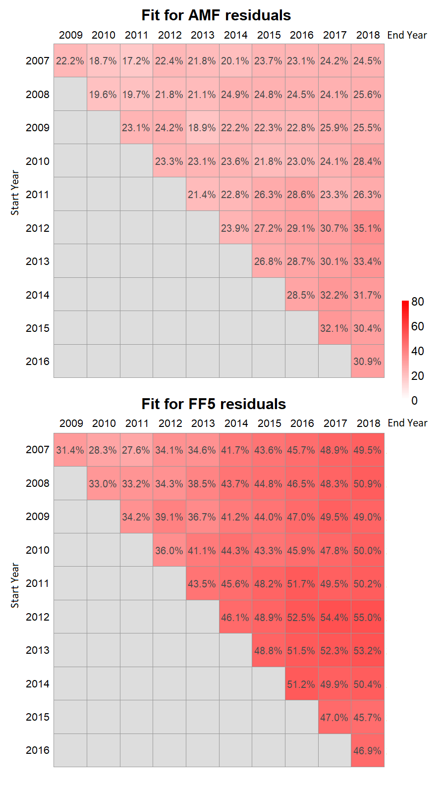
Figure 3.3: Percentage of stocks where the model in Equation (3.30) has significantly better fit compared to Equation (3.30) for each time period. The y-axis is the start year of each time period and the x-axis is the end year. The percentage in each grid is the percentage of stocks with FDR Q-value less than 0.05.

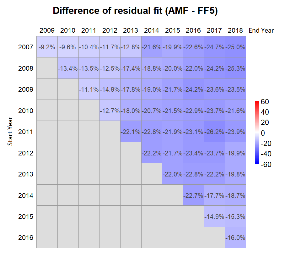
Figure 3.4: Difference of the two heatmaps in Figure 3.3. Each grid is the percentage in AMF model minus the percentage in FF5 model shown in Figure 3.3.

Finally, comparing the results for AMF residuals and FF5 residuals, it is clear that AMF can capture more significant basis assets and leave less information in the residuals compared to the FF5. From Figure 3.4 we know that the percentage of stocks that can be better fitted in the second half time period is always much less for AMF compared to FF5. This indicates that AMF is more powerful than FF5 in capturing useful basis assets.p

3.4.4 Time-invariance Test in Non-Linear GAM Setting

Instead of testing the time-invariance of the $\beta$’s based on a linear model, we can test based on the Generalized Additive Model (GAM). This is a more strict test, since this tests not only on the time-invariance of the $\beta$’s, but the linearity of pthem as well. We first fit a Time-Varying Coefficient model as a special case of the Generalized Additive Model (GAM). The equation can be written as:

$$\Delta\bm{Y}_{i}=\Delta\bm{V}_{S_{i}}[\bm{\beta}_{i}(t)]_{S_{i}}+\Delta\bm{\epsilon}_{i}$$ (3.31)

where $t$ is the time. Note that the only difference between Equation (3.31) and Equation (3.16) is whether we allow $\beta$’s to be functions of time $t$. The GAM model estimate each $\beta$ as a combination of splines or kernels with regard to $t$. This can be done by the gam() function in the R package mgcv.

After that, do a variance analysis (ANOVA) test between the GAM model in Equation (3.31) and the linear model in Equation (3.16) where each $\bm{\beta}_{i}$ are constants over time. In this way, we will get a p-value for each stock. Similar to the section before, we adjust the p-values by the Benjamini-Hochberg-Yekutieli (BHY) [8] method to account for the False Discovery Rate (FDR). We report the percentage of stocks with Q-values less than 0.05 in Figure 3.5.

Figure 3.5 reports the percentage of stocks with time-varying beta using the time-invariance test in a nonlinear GAM setting for each time period. The y-axis is the start year of each time period and the x-axis is the end year of the time period. The percentage in each grid is the percentage of stocks with FDR Q-value less than 0.05 in the ANOVA test comparing the models in Equation (3.31) and (3.16). The larger the percentage is, the darker the grid will be. The upper heatmap is the result of the AMF model, while the bottom heatmap is the result of the FF5 model.

Similarly, by comparing the different skew-diagonals, we can see that both models are more stable in short time periods. AMF outperforms the FF5 in all time periods, which is also shown in Figure 3.6. The Figure 3.6 is the difference between the percentage in two heatmaps in Figure 3.5 (AMF - FF5). All the grids are blue, indicating that AMF is more stable than FF5 in all periods in the GAM setting.

However, comparing the results from GAM and the results in the previous Section 3.4.2, we do find that the GAM test is more strict than the linear test. For any period and both AMF and FF5 models, more companies are shown to have time-varying $\beta$’s in the GAM test, although AMF still outperforms the FF5.

Note that this may not necessarily mean that the $\beta$’s are time-varying in all periods in both tests, since it is really easy for GAM to overfit, especially in short periods. To be more specific, the number of observations for 3 year time periods is $n=156$. For the FF5 model, there are 5 basis assets. For the AMF model, there are sometimes more basis assets selected. For each basis assets, the GAM model selects some splines or kernels, say 10 splines, which can easily boom the real dimension of parameters to $p=5\times 10=50$, which is already too large for regression with $n=156$ observations. In other words, the number of parameters is still too close to the number of observations. Also, these new variables can be highly correlated, making the fitting more unstable. Therefore, some of these GAM fittings may have severe overfitting.

Therefore, the testing based on the GAM model in this section is explorative. Considering this high-dimensional issue, penalization and constraints need to be introduced to traditional GAM for our application. This extension is left for future research.

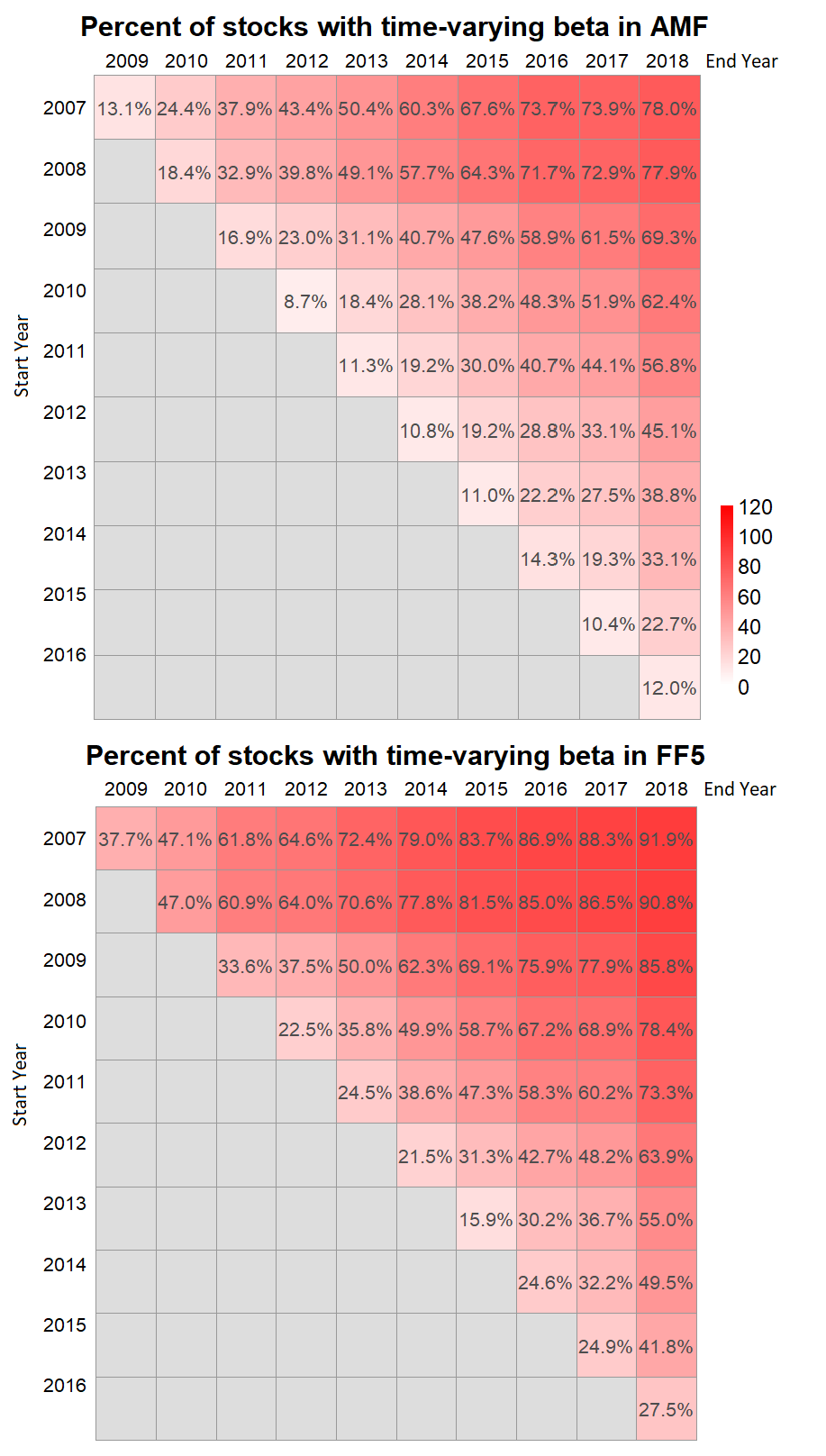
Figure 3.5: Percentage of stocks with time-varying beta using the time-invariance test in a non-linear GAM setting for each time period. The y-axis is the start year of each time period and the x-axis is the end year. The percentage in each grid is the percentage of stocks with FDR Q-value less than 0.05 in Section 3.4.2 ANOVA test comparing the models in Equation (3.31) and (3.16).

Figure 3.6: Difference of the two heatmaps in Figure 3.5 to compare AMF and FF5. Each grid is the percent of time-varying stocks in AMF model minus the percent of time-varying stocks in FF5 model shown inp Figure 3.5.

3.5 Conclusion

The purpose of this paper is to test the multi-factor beta model implied by the generalized arbitrage pricing theory (APT) and the Adaptive Multi-Factor (AMF) model with the Groupwise Interpretable Basis Selection (GIBS) algorithm, without imposing the exogenous assumption of constant betas. The intercept (arbitrage) tests show that there are no significant non-zero intercepts in either AMF or FF5 model, which validates the 2 models.

We do the time-invariance tests for the $\beta$’s for both the AMF model and the FF5 in various periods. We show that the constant-beta assumption holds in the AMF model in all periods with a length of less than 6 years and is quite robust regardless of the start year. However, even for short periods, FF5 sometimes gives very unstable estimation, especially in the financial crisis. This indicates that AMF is more insightful and can capture the risk-factors to explain the market shift during the financial crisis.

For periods with length longer than 6 years, both AMF and FF5 fail to provide time-invariance $\beta$’s. However, the $\beta$’s estimate by the AMF is more time-invariant than the FF5 for nearly all periods. This shows the superior performance of the AMF model.

Considering the two results above, using the dynamic AMF model with a decent rolling window (such as 5 years) is more powerful and stable than the FF5 model.

Chapter 4 Low-volatility Anomaly and the Adaptive Multi-Factor Model

4.1 Introduction

This paper relates to two branches of the asset pricing literature. The first is multi-factor model estimation based on Ross’ (1976) [54] Arbitrage Pricing Theory (APT) and Merton’s (1973) [50] Inter-temporal Capital Asset Pricing Model (ICAPM). The second is the growing literature related to the low-risk anomaly. The purpose of this paper to understand the low-risk anomaly. The low-risk anomaly is the empirical observation that stocks with lower risk yield higher returns than stocks with higher risk. Here risk is quantified as either a security’s return volatility or a security’s beta as derived from a Capital Asset Pricing Model (CAPM). This paper focuses only on the low-volatility anomaly.

To study this anomaly, we use the Adaptive Multi-Factor (AMF) model developed in Zhu et al. (2018) [69] which includes both the APT and ICAPM are special cases. The AMF is derived under a weaker set of assumptions. Its three main benefits are: 1) it is consistent with a large number of risk factors being needed to explain all security returns, 2) yet, the set of risk factors is small for any single security and different for different securities, and 3) the risk factors are traded. These benefits imply that the underlying model estimated is more robust than those used in the existing literature.

The low-risk anomaly contradicts accepted APT or CAPM theories that higher risk portfolios earn higher returns. The low-risk anomaly is not a recent empirical finding but an observation documented by a large body of literature dating back to the 1970s. Despite its longevity, the academic community differs over the causes of the anomaly. The two main explanations are: 1) it is due to leverage constraints that retail, pension and mutual fund investors face which limits their ability to generate higher returns by owning lower risk stocks, and 2) it is due to behavioral biases ranging from the lottery demand for high beta stocks, beating index benchmarks with a limits to arbitrage, and the sell side analysts over-bias on high volatility stocks’ earnings.

The first explanation can be traced back to Black et al. (1972) [11] who showed empirically using stock returns from 1926 to 1966 that expected excess returns on high-beta assets are lower than and that expected excess returns on low-beta stocks are larger than those suggested by the CAPM. In a follow-up paper, accounting for borrowing constraints, Black (1972) [10] proved that the slope of the line between expected returns and $\beta$ must be smaller than when there are no borrowing restrictions. More recently, Frazzini and Pedersen (2014) [22]document the low-beta anomaly in 20 international equity markets and across assets classes including Treasury bonds, corporate bonds, and futures. They argue that investors facing leverage and margin constraints increase the prices of high-beta assets, which generates lower alphas. They show that the Betting Against Beta (BAB) factor, which is long leveraged low-beta assets and short high beta assets, yields positive risk adjusted returns. Ang et al. (2006) [2] find that stocks with high-idiosyncratic volatility after controlling for size, book-to-market, momentum, liquidity effects, and market-wide volatility risk (VIX) earn lower absolute and risk-adjusted returns than stocks with lower-idiosyncratic volatility. Ang et al. (2009) [3] also show that there is a strong comovement in the anomaly across 27 developed markets which implies that easily diversifiable factors cannot explain the out performance of a low idiosyncratic volatility portfolio.

The behavioral explanations (see Baker et al. (2011) [5]) are that irrational investor preferences for lottery-like stocks (more attention is triggered if you talk about Tesla (TSLA) versus Procter & Gamble at a party) and an overconfidence bias pushes the prices of high risk stocks above their fundamentals. Second, because institutional investors have a mandate to outperform some market weighted index, they also over emphasize investments in high-risk stocks. By increasing the beta exposure of their portfolio in this way, they are more likely to beat the benchmark in a rising market. And, due to limits to arbitrage, ”smart money” is not able to arbitrage away this low-risk anomaly. Providing additional support for this explanation, Bali et al. (2017) [6] show that a proxy for lottery demand stocks (the average of the five highest daily returns in a given month) explains this low-beta anomaly. Hong and Sraer (2016) [27] provide an equilibrium model consistent with this behavior. Last, it is also argued that the low-risk anomaly is tied to analyst earnings reports because high-risk stocks are characterized with more inflated sell side analyst’s earnings growth forecasts which produce an investor overreaction and yields lower returns as shown in Hsu et al. (2013) [28].

In this paper we study the low-volatility anomaly from a new perspective based on the Adaptive Multi-Factor (AMF) model proposed in the paper by Zhu et al. (2018) [69] using the recently developed Generalized Arbitrage Pricing Theory (see Jarrow and Protter (2016) [35]). In Zhu et al. (2018) [69], basis assets (formed from the collection of Exchange Traded Funds (ETF)) are used to capture risk factors in realized returns across securities. Since the collection of basis assets is large and highly correlated, high-dimension methods (including the LASSO and prototype clustering) are used. This paper employs the same methodology to investigate the low-volatility anomaly. We find that high-volatility and low-volatility portfolios load on different basis assets, which indicates that volatility is not an independent risk. The out-performance of the low-volatility portfolio is due to the (equilibrium) performance of these loaded risk factors. For completeness, we compare the AMF model with the traditional Fama-French 5-factor (FF5) model, documenting the superior performance of the AMF model. A brief review of the high dimensional statistical methods can be found in Section 2.2.

An outline for this paper is as follows. Section 4.2 discusses the estimation methodology, and section 4.3 presents the results. Section 4.4 concludes.

4.2 The Estimation Methodology

This section gives the estimation methodology. We first pick the universe of stocks and ETFs, so that we only focus on the assets that are easy to trade. Then, we form the high and low volatility portfolios and we choose a time period that exhibits the low-volatility anomaly. We will employ the Adaptive Multi-Factor (AMF) asset pricing model with the Groupwise Interpretable Basis Selection (GIBS) algorithm to these two portfolios and analyze the results in a subsequent section.

4.2.1 The Stock and ETF Universe

The data initially consists of all stocks and ETFs available in the Center for Research in Security Prices (CRSP) database. To ensure all our securities are actively traded, we focus on stocks and ETFs with a market capitalization ranking in top 2500. This filter excludes small stocks that are more likely to exhibit the low-volatility anomaly. In addition, we select stocks and ETFs satisfying the following criteria.

1. According to the description of the CRSP database, ETFs should be with a Share Code (SHRCD) 73. We follow this common practice.

2. We excluded American Depositary Receipts (ADR) from our stock universe. Removing the ADR is a common practice in all empirical finance papers and the main reason is that they are not part of the indices. This is achieved by using the Share Code (SHRCD) 10 or 11 from the CRSP dataset.

3. We only choose ETFs and stocks which are listed on the NYSE, AMEX and NASDAQ exchanges. This is obtained with the Exchange Code (EXCHCD) 1, 2 or 3 from the CRSP dataset.

4. For a stock to be included at time t, its return has to be observable at least 80% of trading times in the previous year in order to calculate its volatility. For an ETF to be considered at time t, its return has to be observable during the 3-year regression window before time t.

The number of ETFs in our universe increased rapidly after 2003, see Figure 4.1. To apply the AMF model and GIBS algorithm, we need enough ETFs to form our collection of basis assets. Hence, we begin our analysis in 2003. To understand the dimension of the set of basis assets, we calculate both the GIBS dimension and the Principal Component Analysis (PCA) dimension of the ETFs in our universe. The PCA dimension at time $t$ is defined to be the number of principal components needed to explain 90% of the variance during the previous 3-years. The GIBS dimension is defined to be the number of “representatives” selected using the GIBS algorithm from the basis assets, i.e. the cardinality of the set $U$ in Table 4.1. The GIBS and PCA dimensions of the ETFs across time are shown in Figure 4.2.

Comparing Figures 4.1 and 4.2, we see that the number of ETFs and dimensions increase over this time period. The GIBS and PCA dimension do not increase as fast as the number of ETFs But, the GIBS dimension increases faster than the PCA dimension, suggesting that GIBS is able to pick more basis assets than does the PCA. The reason is that PCA mixes basis assets together in linear combinations, while the GIBS algorithm does not.

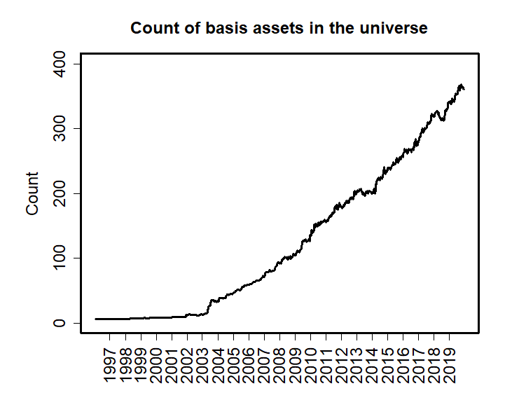
Figure 4.1: Count of the ETFs in the universe.

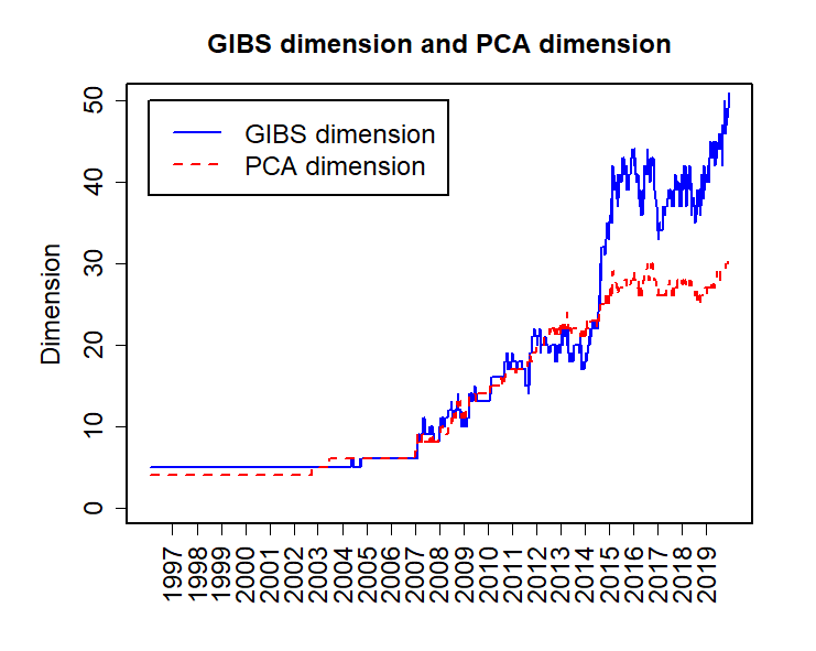
Figure 4.2: GIBS dimension and PCA dimension of ETFs in the universe.

4.2.2 Portfolios and the Low-volatility Anomaly

To study the low-volatility anomaly, we need to form the high- and low-volatility portfolios. To do this, we first calculate the volatility of the stocks in our universe at time $t$ as the standard deviation of their excess returns over the previous year. The excess return is the raw return minus the risk free rate. Using the excess return is a common practice in the empirical finance literature since it removes the risk free rate and focuses on the risk premiums. The high-volatility portfolio is constructed as an equally weighted portfolio using the stocks with the highest 25% volatilities. Similarly, we take the stocks having the lowest 25% volatilities to form the low-volatility portfolio. To avoid a survivorship bias, we include the delisted returns (see Shumway (1997) [55] for more explanation).

We then compare the excess returns of the high- and low-volatility portfolios to verify the existence of the low-volatility anomaly over our sample period. Given the graph, we selected 2008 as the start of the anomaly. Between 2008 - 2018, the low-volatility portfolio had an excess return of 121.4%, which is higher than the 62.5% excess return of the high-volatility portfolio. This documents the existence of the low-volatility anomaly over our sample period. The superior performance of the low-volatility portfolio is manifested in Figure 4.3 which graphs the cumulative value of the two portfolios starting from $1 at the beginning of 2008.

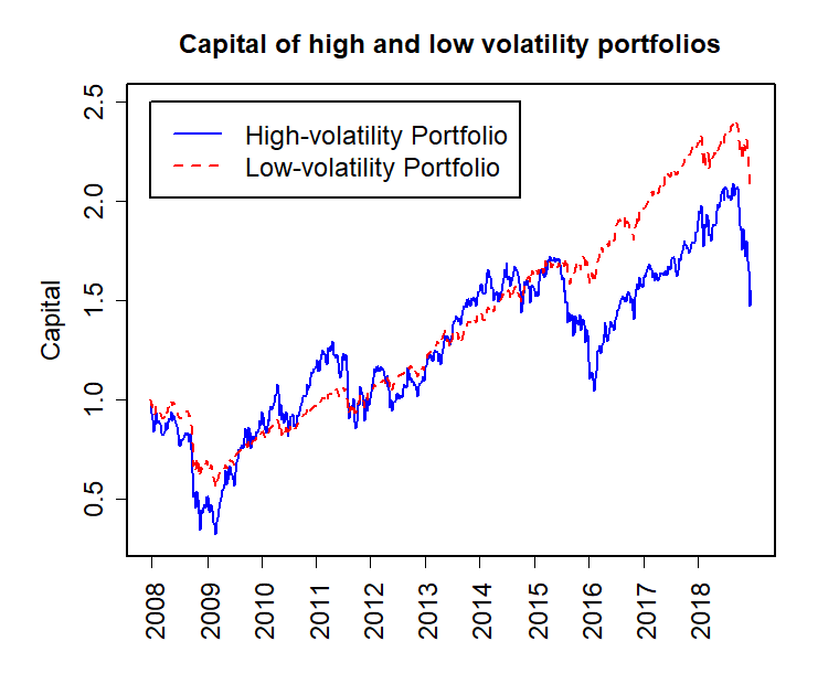
Figure 4.3: Cumulative value of the excess returns from the high- and low-volatility portfolios.

4.2.3 The AMF and GIBS Estimation

This section estimates the Adaptive Multi-Factor (AMF) model based on the Groupwise Interpretable Basis Selection (GIBS) algorithm proposed by Zhu et al. (2018) [69]. Although a brief review of the AMF model and the GIBS algorithm are included in this section, the details can be found in [69]. A sketch of the GIBS algorithm is in Table 4.1 at the end of this section.

To avoid the effects of market micro-structure frictions, we use a weekly horizon. Because the number of ETFs increase over time and the market structure changes during the financial crisis, to approximate stationarity, we pick a 3-year regression window to do the analysis. In addition, because the number of ETFs exceed the number of observations within each regression window, we are in the high-dimensional regime. Therefore, the high-dimensional GIBS algorithm needs to be used to estimate the AMF model. We use a dynamic version of the GIBS algorithm applied to rolling windows. For each week $t$ in 2008 - 2018, we use the time period from 3 years earlier as our current regression window. We use all the ETFs in our universe as described in Section 4.2.1 and the FF5 factors as our basis assets. Then, we apply the GIBS algorithm to select the GIBS determined basis assets and use them to explain the excess returns of the high- and low-volatility portfolios using the AMF model. The following is a more detailed introduction to the AMF model and the GIBS algorithm within each time window.

In the asset pricing theory, given a frictionless, competitive, and arbitrage free market, a dynamic generalization of Ross’s (1976) [54] APT and Merton’s (1973) [50] ICAPM is contained in Jarrow and Protter (2016) [35]. This extension implies that the Adaptive Multi-Factor (AMF) model holds for any security’s return over $[t,t+1]$:

$$R_{i}(t)-r_{0}(t)=\sum_{j=1}^{p}\beta_{i,j}\big{[}r_{j}(t)-r_{0}(t)\big{]}=\bm{\beta}_{i}^{\prime}\cdot[\bm{r}(t)-r_{0}(t)\mathbbm{1}]$$ (4.1)

where $R_{i}(t)$ denotes the return of the i-th security for $1\leq i\leq N$ (where $N$ is the number of securities), $r_{j}(t)$ denotes the return on the j-th basis asset for $1\leq j\leq p$, $r_{0}(t)$ is the risk free rate, $\bm{r}(t)=(r_{1}(t),r_{2}(t),...,r_{p}(t))^{\prime}$ denotes the vector of security returns, $\mathbbm{1}$ is a column vector with every element equal to one, and $\bm{\beta}_{i}=(\beta_{i,1},\beta_{i,2},...,\beta_{i,p})^{\prime}$.

In this paper we are only concerned with the low- and high-volatility portfolios. Let $R_{1}$ denote the raw return of the low-volatility portfolio and $R_{2}$ the raw return of the high-volatility portfolio. To empirically test our model, both an intercept $\alpha_{i}$ and a noise term $\epsilon_{i}(t)$ are added to expression (4.1), i.e.

$$R_{i}(t)-r_{0}(t)=\alpha_{i}+\sum_{j=1}^{p}\beta_{i,j}(t)\big{[}r_{j}(t)-r_{0}(t)\big{]}+\epsilon_{i}(t)=\alpha+\bm{\beta}_{i}^{\prime}[\bm{r}(t)-r_{0}(t)\mathbbm{1}]+\epsilon_{i}(t)$$ (4.2)

where $\epsilon_{i}(t)\overset{iid}{\sim}N(0,\sigma_{i}^{2})$ and $1\leq i\leq N$. The intercept enables the testing for mispriced securities, and the error term allows for noise in the return observations.

As mentioned earlier, using weekly returns over a 3-year time period necessitates the use of high-dimensional statistics. To understand why, consider the following. For a given time period $(t,T)$, letting $n=T-t+1$, we can rewrite expression (4.2) as

$$\bm{R}_{i}-\bm{r}_{0}=\alpha_{i}\mathbbm{1}_{n}+(\bm{r}-\bm{r}_{0}\mathbbm{1}^{\prime}_{p})\bm{\beta}_{i}+\bm{\epsilon}_{i}$$ (4.3)

where $1\leq i\leq N$, $\bm{\epsilon}_{i}\sim N(0,\sigma_{i}^{2}\bm{I}_{n})$ and

$$\bm{R}_{i}=\begin{pmatrix}R_{i}(t)\\ R_{i}(t+1)\\ \vdots\\ R_{i}(T)\end{pmatrix}_{n\times 1},\,\bm{r}_{0}=\begin{pmatrix}r_{0}(t)\\ r_{0}(t+1)\\ \vdots\\ r_{0}(T)\end{pmatrix}_{n\times 1},\,\bm{\epsilon}_{i}=\begin{pmatrix}\epsilon_{i}(t)\\ \epsilon_{i}(t+1)\\ \vdots\\ \epsilon_{i}(T)\end{pmatrix}_{n\times 1}$$

$$\bm{\beta}_{i}=\begin{pmatrix}\beta_{i,1}\\ \beta_{i,2}\\ \vdots\\ \beta_{i,p}\end{pmatrix}_{p\times 1},\,\bm{r}_{i}=\begin{pmatrix}r_{i}(t)\\ r_{i}(t+1)\\ \vdots\\ r_{i}(T)\end{pmatrix}_{n\times 1},\,\bm{r}(t)=\begin{pmatrix}r_{1}(t)\\ r_{2}(t)\\ \vdots\\ r_{p}(t)\end{pmatrix}_{p\times 1}\,$$

$$\bm{r}_{n\times p}=(\bm{r}_{1},\bm{r}_{2},...,\bm{r}_{p})_{n\times p}=\begin{pmatrix}\bm{r}(t)^{\prime}\\ \bm{r}(t+1)^{\prime}\\ \vdots\\ \bm{r}(T)^{\prime}\end{pmatrix}_{n\times p},\,\bm{R}=(\bm{R}_{1},\bm{R}_{2},...,\bm{R}_{N})$$ (4.4)

Recall that the coefficients $\beta_{ij}$ are assumed to be constants. This assumption is only reasonable when the time period $(t,T)$ is small (say 3 years), so the number of observations is $n\approx 150$. However, the number of of basis assets $p$, is around 300 in recent years, implying that the independent variables exceed the observations.

Because of this high-dimension problem and the high-correlation among the basis assets, traditional methods fail to give an interpretable and systematic way to fit the Adaptive Multi-Factor (AMF) model. Therefore, we employ the Groupwise Interpretable Basis Selection (GIBS) algorithm to select the basis assets set $S\subseteq\{1,2,...,p\}$ (the derivation of $S$ is provided later). Then, the model becomes

$$\bm{R}_{i}-\bm{r}_{0}=\alpha_{i}\mathbbm{1}_{n}+(\bm{r}_{S}-(\bm{r}_{0})_{S}\mathbbm{1}^{\prime}_{p})(\bm{\beta}_{i})_{S}+\bm{\epsilon}_{i}.$$ (4.5)

The notation $\bm{r}_{S}$ denotes the columns in the matrix $\bm{r}_{n\times p}$ indexed by the index set $S\subseteq\{1,2,...,p\}$, and $(\bm{r}_{0})_{S}$ denotes the elements in the vector $(\bm{r}_{0})_{n\times 1}$ indexed by the index set $S\subseteq\{1,2,...,p\}$. We will use this notation for any matrices, vectors and indices sets throughout this paper. An example of expression (4.5) is the Fama-French (2015) [20] 5-factor (FF5) model where all of the basis assets are risk-factors, earning non-zero expected excess returns. However, FF5 assumes that the number of risk-factors is small and common to all the securities, whereas the AMF and GIBS does not.

Next, we give a brief review of the GIBS algorithm. For notation simplicity, denote

$$\bm{Y}_{i}=\bm{R}_{i}-\bm{r}_{0}\,,\quad\bm{X}_{i}=\bm{r}_{i}-\bm{r}_{0}\,,\quad\bm{Y}=\bm{R}-\bm{r}_{0}\,,\quad\bm{X}=\bm{r}-\bm{r}_{0}$$ (4.6)

where the definitions of $\bm{R}_{i},\,\bm{R},\,\bm{r}_{i},\,\bm{r}$ are in equations (4.3 - 4.4). Let $\bm{r}_{1}$ denote the market return. It is easy to check that most of the ETF basis assets $\bm{X}_{i}$ are correlated with $\bm{X}_{1}$ (the market return minus the risk free rate). We note that this pattern is not true for the other four Fama-French factors. Therefore, we first orthogonalize every other basis asset to $\bm{X}_{1}$. By orthogonalizing with respect to the market return, we avoid choosing redundant basis assets similar to it and also increase the accuracy of fitting. Note that for the Ordinary Least-Square (OLS) regression, projection does not affect the estimation since it only affects the coefficients, not the estimated $\bm{\hat{y}}$. However, in high-dimension methods such as LASSO, projection does affect the set of selected basis assets because it changes the magnitude of shrinking. Thus, we compute

$$\bm{\widetilde{X}}_{i}=(\bm{I}-P_{\bm{X}_{1}})\bm{X}_{i}=(\bm{I}-\bm{X}_{1}(\bm{X}^{\prime}_{1}\bm{X}_{1})^{-1}\bm{X}_{1}^{\prime})\bm{X}_{i}\qquad\text{where}\quad 2\leq i\leq p_{1}$$ (4.7)

where $P_{\bm{X}_{1}}$ denotes the projection operator, and $p_{1}$ is the number of columns in $\bm{X}_{n\times p_{1}}$. Denote the vector

$$\bm{\widetilde{X}}=(\bm{X}_{1},\bm{\widetilde{X}}_{2},\bm{\widetilde{X}}_{3},...,\bm{\widetilde{X}}_{p_{1}}).$$ (4.8)

Note that this is equivalent to the residuals after regressing other basis assets on the market return minus the risk free rate.

The transformed ETF basis assets $\bm{\widetilde{X}}$ still contain highly correlated members. We first divide these basis assets into categories $A_{1},A_{2},...,A_{k}$ based on a financial characterization. Note that $A\equiv\cup_{i=1}^{k}A_{i}=\{1,2,...,p_{1}\}$. The list of categories with more descriptions can be found in Appendix C. The categories are (1) bond/fixed income, (2) commodity, (3) currency, (4) diversified portfolio, (5) equity, (6) alternative ETFs, (7) inverse, (8) leveraged, (9) real estate, and (10) volatility.

Next, from each category we need to choose a set of representatives. These representatives should span the categories they are from, but also have low correlation with each other. This can be done by using the prototype-clustering method with a distance measure defined by equation (2.1), which yield the “prototypes” (representatives) within each cluster (intuitively, the prototype is at the center of each cluster) with low-correlations.

Within each category, we use the prototype clustering methods previously discussed to find the set of representatives. The number of representatives in each category can be chosen according to a correlation threshold. This gives the sets $B_{1},B_{2},...,B_{k}$ with $B_{i}\subset A_{i}$ for $1\leq i\leq k$. Denote $B\equiv\cup_{i=1}^{k}B_{i}$. Although this reduction procedure guarantees low-correlation between the elements in each $B_{i}$, it does not guarantee low-correlation across the elements in the union $B$. So, an additional step is needed, in which is prototype clustering on $B$ is used to find a low-correlated representatives set $U$. Note that $U\subseteq B$. Denote $p_{2}\equiv\#U$.

Recall from the notation definition in equation 4.12 that $\bm{\widetilde{X}}_{U}$ means the columns of the matrix $\bm{\widetilde{X}}$ indexed by the set $U$. Since basis assets in $\bm{\widetilde{X}}_{U}$ are not highly correlated, a LASSO regression can be applied. By equation (2.6), we have that

$$\bm{\widetilde{\beta}}_{i}=\underset{\bm{\beta}_{i}\in\mathbb{R}^{p},(\bm{\beta}_{i})_{j}=0(\forall j\in U^{c})}{\arg\min}\left\{\frac{1}{2n}\left\|\bm{Y}_{i}-\bm{\widetilde{X}}_{U}(\bm{\beta}_{i})_{U}\right\|_{2}^{2}+\lambda\left\|\bm{\beta}_{i}\right\|_{1}\right\}$$ (4.9)

where $U^{c}$ denotes the complement of $U$. However, here we use a different $\lambda$ as compared to the traditional LASSO. Normally the $\lambda$ of LASSO is selected by cross-validation. However this will overfit the data as discussed in the paper Zhu et al. (2018) [69]. So here we use a modified version of the $\lambda$ selection rule and set

$$\lambda=\max\{\lambda_{1se},min\{\lambda:\#supp(\bm{\widetilde{\beta}}_{i})\leq 20\}\}$$ (4.10)

where $\lambda_{1se}$ is the $\lambda$ selected by the “1se rule”. The “1se rule” gives the most regularized model such that error is within one standard error of the minimum error achieved by the cross-validation (see [23, 56, 60]). Therefore we can derive the the set of basis assets selected as

$$S_{i}\equiv supp(\bm{\widetilde{\beta}}_{i})$$ (4.11)

Next, we fit an Ordinary Least-Square (OLS) regression on the selected basis assets, to estimate $\bm{\hat{\beta}}_{i}$, the OLS estimator from

$$\bm{Y}_{i}=\alpha_{i}\mathbbm{1}_{n}+\bm{X}_{S_{i}}(\bm{\beta}_{i})_{S_{i}}+\bm{\epsilon}_{i}.$$ (4.12)

Note that $supp(\bm{\hat{\beta}}_{i})\subseteq{S}_{i}$. The adjusted $R^{2}$ is obtained from this estimation. Since we are in the OLS regime, significance tests can be performed on $\bm{\hat{\beta}}_{i}$. This yields the significant set of coefficients

$$S_{i}^{*}\equiv\{j:P_{H_{0}}(|\bm{\beta}_{i,j}|\geq|\bm{\hat{\beta}}_{i,j}|)<0.05\}\quad\text{where}\quad H_{0}:\text{True value}\,\,\bm{\beta}_{i,j}=0.$$ (4.13)

Note that the significant basis asset set is a subset of the selected basis asset set. In another words,

$$S_{i}^{*}\subseteq supp(\bm{\hat{\beta}}_{i})\subseteq S_{i}\subseteq\{1,2,...,p\}.$$ (4.14)

Then we look at the significant basis assets for the high- and the low-volatility portfolios separately by creating heatmaps. Each heatmap presents the percentage of selected factors in all of the ETF sectors.

A sketch of the GIBS algorithm is shown in Table 4.1. Recall from the notation definition in equation 4.12 that for an index set $S\subseteq\{1,2,...,p\}$, $\bm{\widetilde{X}}_{S}$ means the columns of the matrix $\bm{\widetilde{X}}$ indexed by the set $S$.

The Groupwise Interpretable Basis Selection (GIBS) algorithm
Inputs: Stocks to fit $\bm{Y}$ and basis assets $\bm{X}$.
1. Derive $\bm{\widetilde{X}}$ using $\bm{X}$ and the Equation (4.7, 4.8).
2. Divide the transformed basis assets $\bm{\widetilde{X}}$ into k groups $A_{1},A_{2},\cdots A_{k}$ using a
financial interpretation.
3. Within each group, use prototype clustering to find prototypes $B_{i}\subset A_{i}$.
4. Let $B=\cup_{i=1}^{k}B_{i}$, use prototype clustering in B to find prototypes $U\subset B$.
5. For each stock $\bm{Y}_{i}$, use a modified version of LASSO to reduce $\bm{\widetilde{X}}_{U}$
to the selected basis assets $\bm{\widetilde{X}}_{S_{i}}$
6. For each stock $\bm{Y}_{i}$, fit linear regression on $\bm{X}_{S_{i}}$.
Outputs: Selected factors $S_{i}$, significant factors $S_{i}^{*}$, and coefficients in step 6.

Table 4.1: The sketch of Groupwise Interpretable Basis Selection (GIBS) algorithm

We repeat this estimation process for all of the 3 year rolling regression windows ending with weeks in 2008 - 2018 (the time period we found in Section 4.2.2 with the low-volatility anomaly). Finally, we compare the significant basis assets selected for the high- and low-volatility portfolios. The results are given in the following Section 4.3. Some details can be found in [37].

4.3 Estimation Results

This section provides the results from our regressions employing both the FF5 and the AMF model.

4.3.1 Residual Analysis: Can FF5 explain the low-volatility anomaly?

We first look at the time series plot of the cumulative capital from investing in the high- and low-volatility portfolios. Figure 4.3 in Section 4.2.2 shows the cumulative capital from the excess returns for both portfolios from 2008 to 2018. As evidenced in these graphs, the two portfolios have different volatilities and the low-volatility portfolio outperforms the high-volatility portfolio.

Next, we calculate the cumulative capital from investing in the residual returns of the high- and the low-volatility portfolios. Figure 4.5 plots the FF5 model and Figure 4.5 plots the AMF model. Comparing Figures 4.3, 4.5, and 4.5, it is clear that the low-volatility anomaly is more pronounced in the excess returns as compared to the residuals. It is still obvious in the FF5 residuals, however, it almost disappears in the AMF residuals.

Formally, we can test for the differences between the cumulative capitals from these two portfolios. Since they have different volatilities, we use Welch’s Two-sample t-test corrected for unequal variances. The hypotheses are

$$H_{0}:\mu_{l}\leq\mu_{h}\qquad H_{A}:\mu_{l}>\mu_{h}$$ (4.15)

where $\mu_{l}$ indicates the capital of the low-volatility portfolio, and the $\mu_{h}$ indicates the capital of the high-volatility portfolio. We do 3 tests where the cumulative capital is calculated with the excess returns, the residual returns from FF5, and the residual returns from AMF. If we reject the null-hypothesis $H_{0}$, then there is strong evidence that the low-volatility anomaly exists.

The p-values of the tests are reported in the parentheses in Table 4.2. In the Table 4.2, the first row is the excess return, the second row is the FF5 residual return, and the third row is the AMF residual return. The first column gives the return to the low-volatility portfolios from 2008 - 2018. The second column is that of the high-volatility portfolios. The third column reports the difference between the two portfolios and gives the p-values of the tests in equation (4.15).

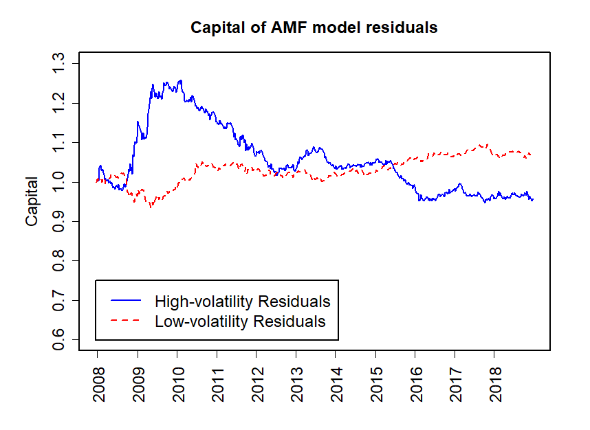
Figure 4.4: Cumulative capital plot of the FF5 residuals of the high-and low-volatility portfolios.

Figure 4.5: Cumulative capital plot of the AMF residuals of the high- and low-volatility portfolios.

	Low Portfolio	High Portfolio	Low - High (P value)
Excess return	1.21	0.62	0.59 ($1.17\times 10^{-5}$)
FF5 residual return	-0.13	-0.31	0.18 ($9.25\times 10^{-95}$)
AMF residual return	-0.05	-0.18	0.12 (1.00)

Table 4.2: Residual analysis comparing the FF5 and AMF models.

The p-value of the FF5 residual is still close to 0, rejecting the null hypothesis, thereby indicating that the low-volatility anomaly still exists after adjusting for risk using the FF5 model. In another words, the FF5 model cannot explain the low-volatility anomaly. However, the p-value of the AMF residual is close to 1, which implies that the low-volatility anomaly is not significant after adjusting for risk with the AMF model. Thus, the AMF model explains the low-volatility anomaly. Indeed, as we will see in Section 4.3.2 below, the AMF model shows that the two portfolios load on different basis assets (and implied risk factors). It is the (equilibrium) performance of these factors underlying the low-volatility portfolio that generates the low-volatility anomaly. Because the FF5 model makes the strong assumption that every security loads on the same 5 factors, it is not able to capture the low-volatiity risk premium differences. This highlights the superior performance of the AMF model.

4.3.2 Factor Comparisons

In this section we compare the significant basis assets or “factors” selected by the GIBS algorithm for the two high- and low-volatility portfolios over 2008 - 2018. Figures 4.7 and 4.7 show the percentage of the significant factors for each ETF class selected by the GIBS algorithm for the low- and high-volatility portfolios each half-year across 2008 - 2018 (see Appendix C for more details on the ETF classifications).

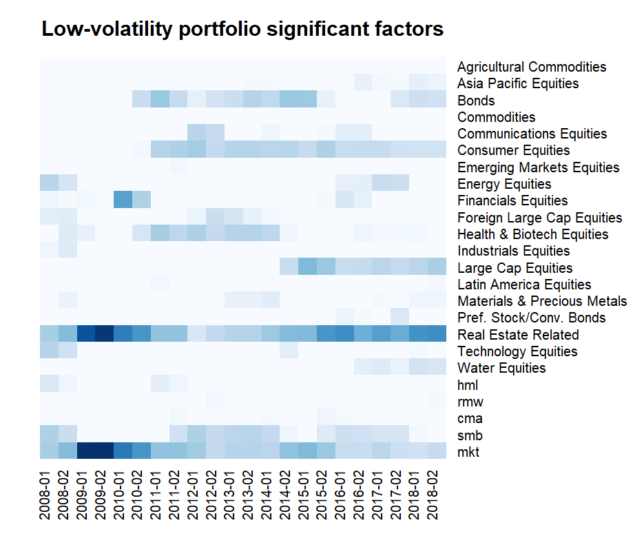
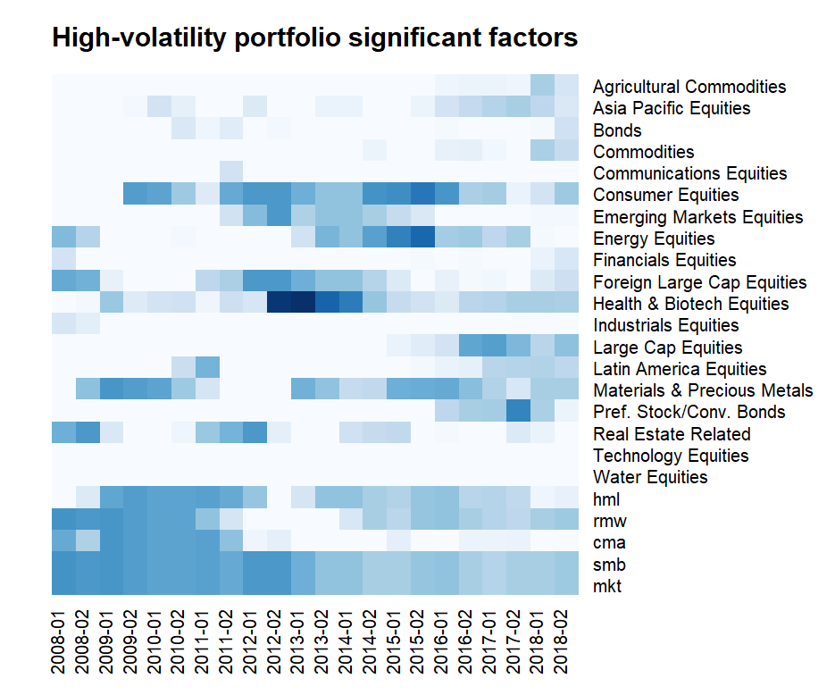
Figure 4.6: Heatmap for the low-volatility portfolio selected factors.

Figure 4.7: Heatmap for the high-volatility portfolio selected factors

As evidenced in the figures, the two portfolios load on very different factors. The low-volatility portfolio is mainly related to the ETFs in Bonds, Consumer Equities, and Real Estate. This is intuitive because bonds and real estate are of lower risk. Among the FF5 factors, the low-volatility portfolio only relates to the market return and the SMB factor. For the high-volatility portfolio, it mainly loads on ETFs in Materials & Precious metals, Consumer Equities, Health & Biotech Equities, and all the FF5 factors, except CMA. The common factors for both portfolios are the market return, the SMB factor, and the Consumer Equity ETFs. Consequently, the out-performance of low-volatility portfolio is due to the different factor loadings, and reflects the differential performance of Bonds and Real Estate relative to materials, precious metals, and the healthcare industry.

Next, we provide a statistical test of whether the two volatility portfolios load on the same factors. Recalling the notation in equation 4.6, denote $\bm{Y}_{1}$ as the excess return to the low-volatility portfolio, and denote $\bm{Y}_{2}$ as the excess return to the high-volatility portfolio over the estimation period. From equation (4.11), denote $S_{1}$ and $S_{2}$ as the basis assets selected by GIBS for the low- and high-volatility portfolios, respectively. Then we let

$$\bm{Z}=\begin{pmatrix}\bm{Y}_{1}\\ \bm{Y}_{2}\end{pmatrix}_{2n\times 1},\,\bm{W}=\begin{pmatrix}\bm{X}\\ \bm{X}\end{pmatrix}_{2n\times 1},\,S=S_{1}\cup S_{2}$$ (4.16)

$$\bm{W}_{S}=\begin{pmatrix}\bm{X}_{S}\\ \bm{X}_{S}\end{pmatrix}_{2n\times 1},\,\bm{h}=\begin{pmatrix}\bm{0}_{n\times 1}\\ \mathbbm{1}_{n\times 1}\end{pmatrix}_{2n\times 1}$$ (4.17)

The vector $\bm{h}$ is an indicator vector which takes the value 1 for the high-volatility portfolio returns and 0 elsewhere.

The testing for the difference between the basis assets selected by the two volatility portfolios can be transformed to a testing for the significance of the interaction between $\bm{h}$ and the selected factors $\bm{W}_{S}$. We fit two models

$$\text{Model 1: }\bm{Z}=\bm{W}_{S}\bm{\beta}_{S}+\bm{\epsilon}$$ (4.18)

$$\text{Model 2: }\bm{Z}=\bm{W}_{S}\bm{\beta}_{S}+\left[\bm{W}_{S}\odot(\bm{h}\mathbbm{1}^{\prime}_{2n})\right]\bm{\gamma}_{S}+\bm{\epsilon}$$ (4.19)

where $\odot$ means the element-wise product for two matrices with the same dimension. Under the null hypothesis that the two portfolios have the same coefficients on the same factors, the goodness of fit of model 1 should be same as that of model 2. So we do an ANOVA(Model1, Model2) test to compare the two models. The results are in Table 4.3.

	Res.Df	RSS	Df difference	Sum of Sq	F statistic	Pr($>$F)
Model 1	1139	0.24
Model 2	1130	0.06	9	0.18	355.25	0.000

Table 4.3: The ANOVA test of the difference of the factors for the two portfolios.

The p-value of the test is approximately 0 to 3 decimal places, much smaller than 0.05, which means that the difference between model 1 and model 2 is significant. This is a strong evidence that the two volatility portfolios have different factor loadings, which validates the implications from the heatmap.

Another observation from the heatmaps is that the high-volatility portfolio is related to more basis assets than is the low-volatility portfolio. The number of basis assets selected by the GIBS algorithm and the number of significant basis assets among them is tabulated in Table 4.4 and graphed in Figures 4.9 and 4.9. We see that more basis assets are selected and significant for the high-volatility portfolio. This is intuitive because the larger volatility is generated by the uncorrelated risks of more basis assets in more volatile industries. More significant basis assets come from the ETF factors than from the FF5 factors. On average only 1.54 of the FF5 factors are significant for the low-volatility portfolio and 3.83 of the FF5 factors are significant for the high-volatility portfolio, manifesting a limitation of the FF5 model. Furthermore, most of the ETFs selected by the GIBS algorithm turn out to be significant, indicating that GIBS is more able to find relevant basis assets.

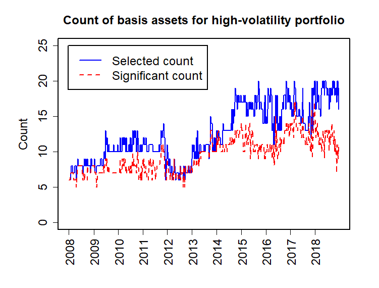
Figure 4.8: The number of selected and significant basis assets for the low-volatility portfolio.

Figure 4.9: The number of the selected and significant basis assets for the high-volatility portfolio.

Portfolio	Select	FF5 Select	ETF Select	Signif.	FF5 Signif.	ETF Signif.
Low	6.96	1.72	5.23	5.82	1.54	4.29
High	12.50	4.12	8.38	9.53	3.83	5.70
Difference	5.54	2.39	3.15	3.71	2.29	1.41

Table 4.4: The number of the selected or significant basis assets / FF5 factors / ETFs for the two volatility portfolios. The “Select” column gives the mean number of basis assets selected by the GIBS algorithm. The “Signif.” column gives the mean number of significant basis assets among the selected ones. The number of the select / significant basis assets is the sum of the number of FF5 factors selected / significant and the ETFs selected / significant. The row “Low” is the results for the low-volatility portfolio, while the row “High” is for high-volatility portfolio. The row “Difference” gives the differences between two portfolios numbers using High - Low.

In summary, our estimation results show that the two volatility portfolios load on very different factors, which implies that volatility is not an independent risk measure, but that it is related to the identified basis assets (risk factors) in the relevant industries. It is the (equilibrium) performance of the loaded factors that results in the low-volatility anomaly and not disequilibrium (abnormal) returns.

4.3.3 Intercept Test

This section provides the tests for a non-zero intercept for both the FF5 and AMF models for both volatility portfolios. This intercept test is a test for abonormal performance, i.e. performance inconsistent with the FF5 and AMF risk models. The null hypothesis is that the $\alpha$’s in equation 4.2 are 0.

Figure 4.11 compares the distribution of the intercept test p-values for the FF5 and AMF models for the low-volatility portfolio, while Figure 4.11 is for the high-volatility portfolio. As we can see from the distribution plots, for both portfolios, the AMF model gives much larger p-values than does the FF5 model. Indeed, there are more weeks where a significant non-zero intercept is exhibited with the FF5 model as compared to the AMF model. This suggests that the AMF model is more consistent with market returns than is the FF5 model. However, this difference could be due to the fact that we repeat this test 520 times (520 weeks in 2008 - 2018), and a percentage of the violations will occur and be observed even if the null hypothesis is true. Hence, it is important to control for a False Discovery Rate (FDR).

We adjust for the false discovery rate using the Benjamini-Hochberg-Yekutieli (BHY) procedures [8] since it accounts for any correlation between the intercept tests. Note that the Benjamini-Hochberg (BH) procedure [7] does not account for correlations, and in our case, weekly returns may be correlated. After adjusting for the false discover rate, for all weeks we fail to reject the non-zero hypothesis for both the FF5 and AMF models. The results are in Table 4.5. This evidence is consistent with the low- and high-volatility portfolios exhibiting no abnormal performance over our observation period.

Figure 4.10: Distribution of intercept test p-values for the low-volatility portfolio.

Figure 4.11: Distribution of intercept test p-values for the high-volatility portfolio.

Portfolio	Percentage of Significant Weeks
	FF5 p$<$0.05	AMF p$<$0.05	FF5 FDR q$<$0.05	AMF FDR q$<$0.05
High	30.1%	20.6%	0.00%	0.00%
Low	6.3%	2.6%	0.00%	0.00%

Table 4.5: Intercept Test with control of the False Discovery Rate. The first row is for the high-volatility portfolio, while the second row is for the low-volatility portfolio. The columns are related to p-values and False Discovery Rate (FDR) q-values for the FF5 model and the AMF model. For each column, we listed the percentage of weeks with significant non-zero intercept out of all the weeks in the 2008 - 2018 time period.

4.3.4 In- and Out-of-Sample Goodness-of-fit Tests

This section compares both the In- and the Out-of-Sample Goodness-of-Fit tests for both the FF5 and the AMF model. For the In-Sample Goodness-of-Fit test, for each volatility portfolio, we record the adjusted $R^{2}$’s (see [58]) for both models for each rolling regression. Then, we calculate the mean of the adjusted $R^{2}$’s. The results are in the Table 4.6.

As shown in this table, even though the FF5 model does a good job in fitting the data, the AMF model is able to increase the adjusted $R^{2}$’s. We fit an ANOVA test comparing the FF5 model to the model using all the basis assets selected by GIBS and FF5. For all the rolling-window regressions over 2008 - 2018, the p-value of this ANOVA test is close to 0, less than 0.05. In another words, for all the weeks over 2008 - 2018, the AMF model has a significantly better fit than does the FF5 model, for both the low- and high-volatility portfolios. Since we do the tests 520 times (520 weeks in 2008 - 2018), we again need to adjust for the False Discovery Rate (FDR). However, even after adjusting the false discovery rate using the most strict BHY method accounting for the correlation between weeks, the FDR q-value is still smaller than 0.05 for all of the weeks. This is a strong evidence that the AMF out-performs the FF5.

Portfolio FF5 Adj. $R^{2}$ AMF Adj. $R^{2}$ (change) $p<0.05$ Ratio FDR $q<0.05$ Ratio Low 0.905 0.961 (+6.18%) 100% 100% High 0.931 0.973 (+4.56%) 100% 100%

Table 4.6: In-Sample Goodness-of-Fit Tests.

For the Out-of-Sample Goodness-of-Fit test, we compare the 1-week ahead Out-of-Sample $R^{2}$ for the FF5 and AMF models for both volatility portfolios. The results are in Table 4.7. It seen in the table, the AMF model out-performs the FF5 model in the prediction period, which indicates that the better performance of the AMF model is not due to over-fitting.

Portfolio	FF5 Out-of-Sample $R^{2}$	AMF Out-of-Sample $R^{2}$ (change)
Low	0.951	0.973 (+2.25%)
High	0.973	0.982 (+1.01%)

Table 4.7: Out-of-Sample Goodness-of-Fit Tests.

4.3.5 Risk Factor Determination

The AMF model selects the basis assets that best span a security’s return. Some of these basis assets may not earn risk premium, and therefore, would not contribute to the risk premium earned by the volatility portfolios. This section studies which of the ETF basis assets correspond to risk-factors, i.e. factors that have non-zero expected excess returns.

At the end of our estimation period 2008 - 2018, there are 335 ETFs in the universe. Among them, the GIBS algorithm selects 35 ETF representatives in total. The list of these 35 ETF representatives is contained in Appendix D Table LABEL:tab:_vol_etf_representatives. Therefore, there are $35+5=40$ basis assets considering both the FF5 factors and ETFs together. In another words, $p_{1}=335$ and $p_{2}=40$ in Section 4.2.3. For each of these basis assets we compute the sample mean excess return over our sample period. This is an estimate of the basis assets’ risk premium.

The risk premium estimates for the Fama-French 5 factors are shown in Table 4.8. All of these are non-zero.

Fama-French 5 Factors	Market Return	SMB	HML	RMW	CMAP
Annual Excess Return (%)	13.2	-0.7	-1.7	0.9	-1.7

Table 4.8: Risk Premium of Fama-French 5 factors

The estimated risk premium for the ETFs are in Table 4.9. Out of the 35 ETF representatives selected by the GIBS algorithm, 23 of them have absolute risk premium larger than the minimum of that of the FF5 factors (which is the RMW with absolute risk premium 0.9%). This means that at least $(23+5)/(35+5)=70\%$ basis assets are risk factors in the traditional sense. The list of the 23 ETFs that earns nonn-zero risk premium are listed in Table 4.9.

Risk Pre- ETF name Category mium (%) iShares MSCI Brazil ETF Latin America Equities 44.0 VanEck Vectors Russia ETF Emperging Markets Equities 20.6 iShares Mortgage Real Estate ETF Real Estate 14.2 Invesco Water Resources ETF Water Equities 13.9 Vanguard Financials ETF Financials Equities 13.2 Vanguard FTSE Emerging Markets ETF Emerging Markets Equities 12.3 VanEck Vectors Agribusiness ETF Large Cap Blend Equities 12.3 Industrial Select Sector SPDR Fund Industrials Equities 12.1 iShares Select Dividend ETF Large Cap Value Equities 11.5 Materials Select Sector SPDR ETF Materials 10.9 Vanguard Healthcare ETF Health & Biotech Equities 10.2 iShares U.S. Home Construction ETF Building & Construction 9.5 iShares MSCI Canada ETF Foreign Large Cap Equities 9.4 SPDR Barclays Capital Convertible Bond ETF Preferred Stock/Convertible Bonds 9.2 First Trust Amex Biotechnology Index Health & Biotech Equities 8.1 Vanguard FTSE All-World ex-US ETF Foreign Large Cap Equities 7.5 SPDR Barclays High Yield Bond ETF High Yield Bonds 6.1 Invesco DB Agriculture Fund Agricultural Commodities -5.9 iShares MSCI Japan ETF Japan Equities 5.8 iShares MSCI Malaysia ETF Asia Pacific Equities 5.7 Invesco DB Commodity Index Tracking Fund Commodities 4.9 iShares Gold Trust Precious Metals 4.2 Vanguard Consumer Staples ETF Consumer Staples Equities 3.8

Table 4.9: List of ETFs with large absolute risk premium.

4.4 Conclusion

In this paper we construct high- and low-volatility portfolios within the investable universe to explain the low-volatility anomaly using a new model, the Adaptive Multi-Factor (AMF) model estimated by the Groupwise Interpretable Basis Selection (GIBS) algorithm proposed in the paper by Zhu et al. (2018) [69]. For comparison with the literature, we compare the AMF model with the traditional Fama-French 5-factor (FF5) model. Our estimation shows the superior performance of the AMF model over FF5. Indeed, we show that the FF5 cannot explain the low-volatility anomaly while the AMF can. The AMF results show that the two volatility portfolios load on very different factors, which indicates that the volatility is not an independent measure of risk. It is the performance of the underlying risk factors that results in the low-volatility anomaly. Alternatively stated, the out-performance of the low-volatility portfolio reflects the equilibrium compensation for the risk of its underlying risk factors.

Appendix A Summary of Generalized APT

This appendix provides a summary of the key results from the generalized APT contained in Jarrow and Protter (2016) [35] that are relevant to the empirical estimation and different from the traditional approach to the estimation of factor models. Prior to that, however, we first discuss the traditional approach to the estimation of factor models.

The traditional approach to the estimation of factor models, based on Merton (1973) [50] and Ross (1976) [54], starts with an expected return relation between a risky asset and a finite collection of risk-factors. Merton’s relation is derived from the first order conditions of an investor’s optimization problem, given in expectations. Ross’s relation is derived from a limiting arbitrage pricing condition satisfied by the asset’s expected returns. Given these are expected return relations, the included risk factor’s excess expected returns are all non-zero by construction. These non-zero expected excess returns are interpreted as risk premiums earned for systematic risk exhibited by the risk factors. Jensen’s alpha is then viewed as a wedge between the risky assets expected return and those of the risk factors implying a mispricing in the market.

To get an empirical relation in realized returns for estimation, the traditional approach rewrites these risk-factor expected returns as a realized return less an error. Substitution yields an expression relating a risky asset’s realized return to the realized return’s of the risk factors plus a cumulative error. Since the risk factors do not reflect idiosyncratic risk, the cumulative error in this relation may not satisfy the standard assumptions needed for a regression model. In particular, the error term may be autocorrelated and/or correlated with other idiosyncratic risk terms not included in the estimated equation. Because the estimated relation is derived from a relation involving expectations using risk-factors, the $R^{2}$ of the realized return regression can be small.

Jarrow and Protter (2016) derive a testable multi-factor model in a different and more general setting. With trading in a finite number for risky assets in the context of a continuous time, continuous trading market assuming only frictionless and competitive markets that satisfy no-arbitrage and no dominance, i. e. the existence of an equivalent martingale measure, they are able to derive a no-arbitrage condition satsifed by any trading strategy’s realized returns. Adding additional structure to the economy and then taking expectations yields both Merton’s (1973) [50] and Ross’s (1976) [54] models as special cases.

The generalize APT uses linear algebra to prove the existence of an algebraic basis in the risky asset’s payoff space at some future time T. Since this is is a continuous time and trading economy, this payoff space is infinite dimensional. The algebraic basis at time T constitutes the collection of basis assets. It is important to note that this set of basis assets are tradable. An algebraic basis means that any risky asset’s return can be written as a linear combination of a finite number of the basis asset returns, and different risky assets may have a different finite combination of basis assets explaining their returns. Since the space of random variables generated by the admissible trading strategies is infinite dimensional, this algebraic basis representation of the relevant risks is parsimonious and sparse. Indeed, only a finite number of basis assets in an infinite dimensional space explains any trading strategy’s return process.

No arbitrage, the martingale relation, implies that the same set of basis assets explains any particular risky asset’s realized returns at all earlier times $t\in[0,T]$ as well. This is the no arbitrage relation satisfied by the realized return processes. Adding a non-zero alpha to this relation (Jensen’s alpha) implies a violation of the no-arbitrage condition. This no-arbitrage condition is valid and testable in realized return space.

In contrast to the traditional approach (discussed above), deriving the relation in realized return space implies that the error structure is more likely to satisfy the standard assumptions of regression models. This follows because including basis assets with zero excess expected returns (which are excluded in the traditional approach based on risk-factors) will reduce correlations between the error terms across time and cross-sectionally between the error terms and the other basis assets (independent variables). The result is the estimated equation should have a larger $R^{2}$. After fitting the multi-factor model in realized returns, estimating the relevant basis assets expectations determines which are risk-factors, i.e. which earn a risk premium for systematic risk.

Appendix B Company Classes by SIC Code

The following list of company classes based on the first two digits of Standard Industrial Classification (SIC) code is from the website of United States Department of Labor (https://www.osha.gov/pls/imis/sic_manual.html):

Table B.1: Company classes by the Standard Industrial Classification (SIC) code

Division A	Agriculture, Forestry, And Fishing
Major Group 01	Agricultural Production Crops
Major Group 02	Agriculture production livestock and animal specialties
Major Group 07	Agricultural Services
Major Group 08	Forestry
Major Group 09	Fishing, hunting, and trapping
Division B	Mining
Major Group 10	Metal Mining
Major Group 12	Coal Mining
Major Group 13	Oil And Gas Extraction
Major Group 14	Mining And Quarrying Of Nonmetallic Minerals, Except Fuels
Division C	Construction
Major Group 15	Building Construction General Contractors And Operative Builders
Major Group 16	Heavy Construction Other Than Building Construction Contractors
Major Group 17	Construction Special Trade Contractors
Division D	Manufacturing
Major Group 20	Food And Kindred Products
Major Group 21	Tobacco Products
Major Group 22	Textile Mill Products
Major Group 23	Apparel And Other Finished Products Made From Fabrics And Similar Materials
Major Group 24	Lumber And Wood Products, Except Furniture
Major Group 25	Furniture And Fixtures
Major Group 26	Paper And Allied Products
Major Group 27	Printing, Publishing, And Allied Industries
Major Group 28	Chemicals And Allied Products
Major Group 29	Petroleum Refining And Related Industries
Major Group 30	Rubber And Miscellaneous Plastics Products
Major Group 31	Leather And Leather Products
Major Group 32	Stone, Clay, Glass, And Concrete Products
Major Group 33	Primary Metal Industries
Major Group 34	Fabricated Metal Products, Except Machinery And                     Transportation Equipment
Major Group 35	Industrial And Commercial Machinery And Computer                               Equipment
Major Group 36	Electronic And Other Electrical Equipment And Components, Except Computer Equipment
Major Group 37	Transportation Equipment
Major Group 38	Measuring, Analyzing, And Controlling Instruments; Photographic, Medical And Optical Goods; Watches And Clocks
Major Group 39	Miscellaneous Manufacturing Industries
Division E	Transportation, Communications, Electric, Gas, And Sanitary Services
Major Group 40	Railroad Transportation
Major Group 41	Local And Suburban Transit And Interurban Highway Passenger Transportation
Major Group 42	Motor Freight Transportation And Warehousing
Major Group 43	United States Postal Service
Major Group 44	Water Transportation
Major Group 45	Transportation By Air
Major Group 46	Pipelines, Except Natural Gas
Major Group 47	Transportation Services
Major Group 48	Communications
Major Group 49	Electric, Gas, And Sanitary Services
Division F	Wholesale Trade
Major Group 50	Wholesale Trade-durable Goods
Major Group 51	Wholesale Trade-non-durable Goods
Division G	Retail Trade
Major Group 52	Building Materials, Hardware, Garden Supply, And Mobile Home Dealers
Major Group 53	General Merchandise Stores
Major Group 54	Food Stores
Major Group 55	Automotive Dealers And Gasoline Service Stations
Major Group 56	Apparel And Accessory Stores
Major Group 57	Home Furniture, Furnishings, And Equipment Stores
Major Group 58	Eating And Drinking Places
Major Group 59	Miscellaneous Retail
Division H	Finance, Insurance, And Real Estate
Major Group 60	Depository Institutions
Major Group 61	Non-depository Credit Institutions
Major Group 62	Security And Commodity Brokers, Dealers, Exchanges, And Services
Major Group 63	Insurance Carriers
Major Group 64	Insurance Agents, Brokers, And Service
Major Group 65	Real Estate
Major Group 67	Holding And Other Investment Offices
Division I	Services
Major Group 70	Hotels, Rooming Houses, Camps, And Other Lodging Places
Major Group 72	Personal Services
Major Group 73	Business Services
Major Group 75	Automotive Repair, Services, And Parking
Major Group 76	Miscellaneous Repair Services
Major Group 78	Motion Pictures
Major Group 79	Amusement And Recreation Services
Major Group 80	Health Services
Major Group 81	Legal Services
Major Group 82	Educational Services
Major Group 83	Social Services
Major Group 84	Museums, Art Galleries, And Botanical And Zoological Gardens
Major Group 86	Membership Organizations
Major Group 87	Engineering, Accounting, Research, Management, And Related Services
Major Group 88	Private Households
Major Group 89	Miscellaneous Services
Division J	Public Administration
Major Group 91	Executive, Legislative, And General Government, Except Finance
Major Group 92	Justice, Public Order, And Safety
Major Group 93	Public Finance, Taxation, And Monetary Policy
Major Group 94	Administration Of Human Resource Programs
Major Group 95	Administration Of Environmental Quality And Housing            pPrograms
Major Group 96	Administration Of Economic Programs
Major Group 97	National Security And International Affairs
Major Group 99	Nonclassifiable Establishments

Appendix C ETF Classes and Subclasses

ETFs can be divided into 10 classes, 73 subclasses (categories) in total, based on their financial explanations. The classify criteria are found from the ETFdb database: www.etfdb.com. The classes and subclasses are listed below:

1. Bond/Fixed Income: California Munis, Corporate Bonds, Emerging Markets Bonds, Government Bonds, High Yield Bonds, Inflation-Protected Bonds, International Government Bonds, Money Market, Mortgage Backed Securities, National Munis, New York Munis, Preferred Stock/Convertible Bonds, Total Bond Market.

2. Commodity: Agricultural Commodities, Commodities, Metals, Oil & Gas, Precious Metals.

3. Currency: Currency.

4. Diversified Portfolio: Diversified Portfolio, Target Retirement Date.

5. Equity: All Cap Equities, Alternative Energy Equities, Asia Pacific Equities, Building & Construction, China Equities, Commodity Producers Equities, Communications Equities, Consumer Discretionary Equities, Consumer Staples Equities, Emerging Markets Equities, Energy Equities, Europe Equities, Financial Equities, Foreign Large Cap Equities, Foreign Small & Mid Cap Equities, Global Equities, Health & Biotech Equities, Industrials Equities, Japan Equities, Large Cap Blend Equities, Large Cap Growth Equities, Large Cap Value Equities, Latin America Equities, MLPs (Master Limited Partnerships), Materials, Mid Cap Blend Equities, Mid Cap Growth Equities, Mid Cap Value Equities, Small Cap Blend Equities, Small Cap Growth Equities, Small Cap Value Equities, Technology Equities, Transportation Equities, Utilities Equities, Volatility Hedged Equity, Water Equities.

6. Alternative ETFs: Hedge Fund, Long-Short.

7. Inverse: Inverse Bonds, Inverse Commodities, Inverse Equities, Inverse Volatility.

8. Leveraged: Leveraged Bonds, Leveraged Commodities,
   Leveraged Currency, Leveraged Equities, Leveraged Multi-Asset, Leveraged Real Estate, Leveraged Volati-lity.

9. Real Estate: Global Real Estate, Real Estate.

10. Volatility: Volatility.

In Section 4.3.2, we merged several categories to give a better visualization of the significant factors for each portfolio. The merged categories are

• Bonds: Corporate Bonds, Government Bonds, High Yield Bonds, Total Bond Market, Leveraged Bonds.

• Consumer Equities: Consumer Discretionary Equities, Consumer Staples Equities.

• Real Estate Related: Real Estate, Leveraged Real Estate, Global Real Estate, Utilities Equities,”Building & Construction.

• Energy Equities: Energy Equities, Alternative Energy Equities.

• Materials & Precious Metals: Materials, Precious Metals

• Large Cap Equities: Large Cap Blend Equities, Large Cap Growth Equities, Large Cap Value Equities.

Appendix D Low-Correlated ETF Name Lists

The low-correlated ETF name list in Section 2.4 is in Table LABEL:tab:_amf_etf_representatives.

Table D.1: Low-correlated ETF name list in Section 2.4.

ETF Names	Category
iShares California Muni Bond ETF	California Munis
iShares Emerging Markets Corporate Bond ETF	Corporate Bonds
FlexShares Ready Access Variable Income Fund	Corporate Bonds
Invesco International Corporate Bond ETF	Corporate Bonds
WisdomTree Emerging Markets Corporate Bond Fund	Corporate Bonds
iShares Floating Rate Bond ETF	Corporate Bonds
ProShares Investment Grade-Interest Rate Hedged	Corporate Bonds
iShares iBonds Mar 2020 Corporate ETF	Corporate Bonds
VanEck Vectors Investment Grade Floating Rate ETF	Corporate Bonds
SPDR Barclays Capital Investment Grade Floating Rate ETF	Corporate Bonds
iShares iBonds Mar 2020 Corporate ex-Financials ETF	Corporate Bonds
Vanguard Emerging Markets Government Bond ETF	Emerging Markets Bonds
ProShares Short Term USD Emerging Markets Bond ETF	Emerging Markets Bonds
SPDR Barclays 1-3 Month T-Bill ETF	Government Bonds
iShares Short Treasury Bond ETF	Government Bonds
SPDR Portfolio Short Term Treasury ETF	Government Bonds
SPDR BofA Merrill Lynch Crossover Corporate Bond ETF	High Yield Bonds
VanEck Vectors International High Yield Bond ETF	High Yield Bonds
SPDR Blackstone/ GSO Senior Loan ETF	High Yield Bonds
Highland iBoxx Senior Loan ETF	High Yield Bonds
Invesco Global Short Term High Yield Bond ETF	High Yield Bonds
WisdomTree Interest Rate Hedged High Yield Bond Fund	High Yield Bonds
First Trust Senior Loan Exchange-Traded Fund	High Yield Bonds
PIMCO 0-5 Year High Yield Corporate Bond Index Fund	High Yield Bonds
WisdomTree Negative Duration High Yield Bond Fund	High Yield Bonds
ProShares Inflation Expectations ETF	Inflation-Protected Bonds
WisdomTree Asia Local Debt Fund	International Government Bonds
iShares Ultra Short-Term Bond ETF	Money Market
VanEck Vectors AMT-Free Short Municipal Index ETF	National Munis
Invesco VRDO Tax-Free Weekly ETF	National Munis
Pimco Short Term Municipal Bond Fund	National Munis
VanEck Vectors AMT-Free Intermediate Municipal Index ETF	National Munis
VanEck Vectors Pre-Refunded Municipal Index ETF	National Munis
iShares S&P Short Term AMT-Free Bond ETF	National Munis
SPDR Barclays Short Term Municipal Bond	National Munis
SPDR Barclays Capital Convertible Bond ETF	Preferred Stock or                     Convertible Bonds
iShares International Preferred Stock ETF	Preferred Stock or                     Convertible Bonds
iShares U.S. Preferred Stock ETF	Preferred Stock or                     Convertible Bonds
iShares Short Maturity Bond ETF	Total Bond Market
Invesco Chinese Yuan Dim Sum Bond ETF	Total Bond Market
Franklin Short Duration U.S. Government ETF	Total Bond Market
Invesco CEF Income Composite ETF	Total Bond Market
AdvisorShares Newfleet Multi-Sector Income ETF	Total Bond Market
SPDR SSgA Ultra Short Term Bond ETF	Total Bond Market
WisdomTree Barclays Interest Rate Hedged U.S. Aggregate Bond Fund	Total Bond Market
WisdomTree Barclays Negative Duration U.S. Aggregate Bond Fund	Total Bond Market
PIMCO Enhanced Short Maturity Strategy Fund	Total Bond Market
Invesco DB Agriculture Fund	Agricultural Commodities
Invesco DB Base Metals Fund	Metals
Invesco DB Oil Fund	Oil & Gas
Aberdeen Standard Physical Palladium Shares ETF	Precious Metals
Invesco DB Precious Metals Fund	Precious Metals
Invesco CurrencyShares Swiss Franc Trust	Currency
Invesco CurrencyShares Canadian Dollar Trust	Currency
WisdomTree Brazilian Real Fund	Currency
Invesco DB G10 Currency Harvest Fund	Currency
First Trust Dorsey Wright People’s Portfolio ETF	Diversified Portfolio
Arrow Dow Jones Global Yield ETF	Diversified Portfolio
First Trust Multi-Asset Diversified Income Index Fund	Diversified Portfolio
iShares Moderate Allocation ETF	Diversified Portfolio
Renaissance IPO ETF	All Cap Equities
Invesco Dynamic Leisure and Entertainment ETF	All Cap Equities
VanEck Vectors Israel ETF	All Cap Equities
Invesco Dynamic Media ETF	All Cap Equities
Invesco Cleantech ETF	Alternative Energy Equities
First Trust ISE Global Wind Energy Index Fund	Alternative Energy Equities
VanEck Vectors Global Alternative Energy ETF	Alternative Energy Equities
First Trust NASDAQ Clean Edge Smart Grid Infrastructure Index Fund	Alternative Energy Equities
Invesco WilderHill Progressive Energy ETF	Alternative Energy Equities
WisdomTree India Earnings Fund	Asia Pacific Equities
Vanguard FTSE Pacific ETF	Asia Pacific Equities
First Trust India NIFTY 50 Equal Weight ETF	Asia Pacific Equities
WisdomTree Australia Dividend Fund	Asia Pacific Equities
iShares MSCI Thailand ETF	Asia Pacific Equities
VanEck Vectors Vietnam ETF	Asia Pacific Equities
iShares MSCI Philippines ETF	Asia Pacific Equities
First Trust ISE Chindia Index Fund	Asia Pacific Equities
iShares MSCI China Small-Cap ETF	Asia Pacific Equities
iShares MSCI New Zealand ETF	Asia Pacific Equities
First Trust ISE Global Engineering and Construction ETF	Building & Construction
SPDR S&P Homebuilders ETF	Building & Construction
Invesco Dynamic Building & Construction ETF	Building & Construction
VanEck Vectors ChinaAMC CSI 300 ETF	China Equities
KraneShares CSI China Five Year Plan ETF	China Equities
Invesco Global Agriculture ETF	Commodity Producers         Equities
iShares North American Tech-Multimedia Network            pETF	Communications Equities
iShares U.S. Telecommunications ETF	Communications Equities
First Trust NASDAQ Global Auto Index Fund	Consumer Discretionary       Equities
VanEck Vectors Gaming ETF	Consumer Discretionary       Equities
SPDR S&P Retail ETF	Consumer Discretionary       Equities
Invesco S&P SmallCap Consumer Staples ETF	Consumer Staples Equities
IQ Global Agribusiness Small Cap ETF	Consumer Staples Equities
Vanguard Consumer Staples ETF	Consumer Staples Equities
iShares MSCI Frontier 100 ETF	Emerging Markets Equities
VanEck Vectors Russia Small-Cap ETF	Emerging Markets Equities
Global X FTSE Greece 20 ETF	Emerging Markets Equities
WisdomTree Middle East Dividend Fund	Emerging Markets Equities
VanEck Vectors Egypt Index ETF	Emerging Markets Equities
iShares MSCI Turkey ETF	Emerging Markets Equities
VanEck Vectors Coal ETF	Energy Equities
iShares MSCI Ireland ETF	Europe Equities
VanEck Vectors Poland ETF	Europe Equities
iShares MSCI United Kingdom Small-Cap ETF	Europe Equities
WisdomTree Europe Hedged Equity Fund	Europe Equities
Xtrackers MSCI United Kingdom Hedged Equity Fund	Europe Equities
Global X MSCI Portugal ETF	Europe Equities
First Trust Germany AlphaDEX Fund	Europe Equities
Invesco Global Listed Private Equity ETF	Financials Equities
ProShares Global Listed Private Equity ETF	Financials Equities
Invesco KBW High Dividend Yield Financial ETF	Financials Equities
Invesco DWA Financial Momentum ETF	Financials Equities
SPDR S&P Insurance ETF	Financials Equities
iShares MSCI EAFE ETF	Foreign Large Cap Equities
VanEck Vectors Africa Index ETF	Foreign Large Cap Equities
First Trust S&P International Dividend Aristocrats ETF	Foreign Large Cap Equities
Invesco S&P International Developed Momentum ETF	Foreign Large Cap Equities
Global X MSCI Nigeria ETF	Foreign Large Cap Equities
Global X MSCI Argentina ETF	Global Equities
iShares MSCI Peru ETF	Global Equities
ROBO Global Robotics and Automation Index ETF	Global Equities
Global X Uranium ETF	Global Equities
IQ Hedge Macro Tracker ETF	Global Equities
AdvisorShares Dorsey Wright ADR ETF	Global Equities
SPDR S&P Health Care Services ETF	Health & Biotech Equities
iShares U.S. Pharmaceuticals ETF	Health & Biotech Equities
SPDR S&P Health Care Equipment ETF	Health & Biotech Equities
VanEck Vectors Environmental Services ETF	Industrials Equities
iShares U.S. Aerospace & Defense ETF	Industrials Equities
SPDR MSCI ACWI IMI ETF	Large Cap Blend Equities
Invesco S&P 500 BuyWrite ETF	Large Cap Blend Equities
VanEck Vectors Morningstar Wide Moat ETF	Large Cap Blend Equities
iShares MSCI Israel ETF	Large Cap Blend Equities
Global X NASDAQ 100 Covered Call ETF	Large Cap Growth Equities
AlphaClone Alternative Alpha ETF	Large Cap Growth Equities
Invesco Russell Top 200 Equal Weight ETF	Large Cap Growth Equities
Invesco NASDAQ Internet ETF	Large Cap Growth Equities
Global X MSCI Colombia ETF	Latin America Equities
iShares Global Timber & Forestry ETF	Materials
VanEck Vectors Rare Earth/Strategic Metals ETF	Materials
Global X Lithium ETF	Mid Cap Blend Equities
Invesco Global Water ETF	Mid Cap Growth Equities
Invesco DWA NASDAQ Momentum ETF	Small Cap Growth Equities
iShares North American Tech-Software ETF	Technology Equities
Invesco S&P SmallCap Information Technology ETF	Technology Equities
SPDR S&P Semiconductor ETF	Technology Equities
First Trust NASDAQ CEA Smartphone Index Fund	Technology Equities
iShares Transportation Average ETF	Transportation Equities
Vanguard Utilities ETF	Utilities Equities
SPDR SSGA US Small Cap Low Volatility Index ETF	Volatility Hedged Equity
SPDR SSGA US Large Cap Low Volatility Index ETF	Volatility Hedged Equity
Invesco S&P 500 Downside Hedged ETF	Volatility Hedged Equity
Invesco Water Resources ETF	Water Equities
First Trust ISE Water Index Fund	Water Equities
WisdomTree Managed Futures Strategy Fund	Hedge Fund
IQ Merger Arbitrage ETF	Hedge Fund
Proshares Merger ETF	Hedge Fund
SPDR SSgA Multi-Asset Real Return ETF	Hedge Fund
First Trust Morningstar Managed Futures Strategy Fund	Hedge Fund
IQ Real Return ETF	Hedge Fund
ProShares RAFI Long/Short	Long-Short
IQ Hedge Market Neutral Tracker ETF	Long-Short
FLAG-Forensic Accounting Long-Short ETF	Long-Short
AGFiQ US Market Neutral Anti-Beta Fund	Long-Short
AGFiQ US Market Neutral Size Fund	Long-Short
AGFiQ US Market Neutral Momentum Fund	Long-Short
ProShares Short 7-10 Year Treasury	Inverse Bonds
Short MSCI Emerging Markets ProShares	Inverse Equities
AdvisorShares Ranger Equity Bear ETF	Inverse Equities
ProShares Ultra High Yield	Leveraged Bonds
ProShares Ultra Bloomberg Natural Gas	Leveraged Commodities
ProShares Ultra Yen	Leveraged Currency
Direxion Daily Energy Bull 3X Shares	Leveraged Equities
ProShares Ultra Basic Materials	Leveraged Equities
ProShares Ultra Semiconductors	Leveraged Equities
ProShares Ultra Real Estate	Leveraged Real Estate
SPDR DJ Wilshire International Real Estate ETF	Global Real Estate
ProShares VIX Short-Term Futures ETF	Volatility

The low-correlated ETF name list in Section 4.3.5 is in Table LABEL:tab:_vol_etf_representatives.

Table D.2: Low-correlated ETF name list in Section 4.3.5.

ETF Names	Category
iShares Gold Trust	Precious Metals
iShares MSCI Malaysia ETF	Asia Pacific Equities
Vanguard FTSE All-World ex-US ETF	Foreign Large Cap Equities
iShares MSCI Canada ETF	Foreign Large Cap Equities
VanEck Vectors Agribusiness ETF	Large Cap Blend Equities
Vanguard FTSE Emerging Markets ETF	Emerging Markets Equities
VanEck Vectors Russia ETF	Emerging Markets Equities
PIMCO Enhanced Short Maturity Strategy Fund	Total Bond Market
iShares 3-7 Year Treasury Bond ETF	Government Bonds
SPDR Barclays 1-3 Month T-Bill ETF	Government Bonds
iShares Short Treasury Bond ETF	Government Bonds
iShares U.S. Home Construction ETF	Building & Construction
Alerian MLP ETF	MLPs
SPDR Barclays High Yield Bond ETF	High Yield Bonds
Vanguard Healthcare ETF	Health & Biotech Equities
SPDR Barclays Short Term Municipal Bond	National Munis
Materials Select Sector SPDR ETF	Materials
iShares MSCI Japan ETF	Japan Equities
WisdomTree Japan Hedged Equity Fund	Japan Equities
iShares Mortgage Real Estate ETF	Real Estate
Invesco DB Commodity Index Tracking Fund	Commodities
SPDR S&P Retail ETF	Consumer Discretionary                     Equities
Vanguard Financials ETF	Financials Equities
iShares MSCI Brazil ETF	Latin America Equities
iShares MSCI Mexico ETF	Latin America Equities
iShares Select Dividend ETF	Large Cap Value Equities
Invesco Water Resources ETF	Water Equities
SPDR DJ Wilshire Global Real Estate ETF	Global Real Estate
iShares North American Tech-Software ETF	Technology Equities
Consumer Staples Select Sector SPDR Fund	Consumer Staples Equities
SPDR Barclays Capital Convertible Bond ETF	Preferred Stock /                               Convertible Bonds
Invesco Preferred ETF	Preferred Stock /                               Convertible Bonds
Invesco DB Agriculture Fund	Agricultural Commodities
Industrial Select Sector SPDR Fund	Industrials Equities
SPDR FTSE International Government Inflation-Protected Bond ETF	Inflation-Protected Bonds

References

- [1] Tobias Adrian, Richard K Crump, and Emanuel Moench. Regression based estimation of dynamic asset pricing models. Journal of Financial Economics, 118(2):211–244, 2015.
- [2] Andrew Ang, Robert J Hodrick, Yuhang Xing, and Xiaoyan Zhang. The cross-section of volatility and expected returns. The Journal of Finance, 61(1):259–299, 2006.
- [3] Andrew Ang, Robert J Hodrick, Yuhang Xing, and Xiaoyan Zhang. High idiosyncratic volatility and low returns: International and further us evidence. Journal of Financial Economics, 91(1):1–23, 2009.
- [4] Doron Avramov and Tarun Chordia. Asset pricing models and financial market anomalies. The Review of Financial Studies, 19(3):1001–1040, 2006.
- [5] Malcolm Baker, Brendan Bradley, and Jeffrey Wurgler. Benchmarks as limits to arbitrage: Understanding the low-volatility anomaly. Financial Analysts Journal, 67(1):40–54, 2011.
- [6] Turan G Bali, Stephen J Brown, Scott Murray, and Yi Tang. A lottery-demand-based explanation of the beta anomaly. Journal of Financial and Quantitative Analysis, 52(6):2369–2397, 2017.
- [7] Yoav Benjamini and Yosef Hochberg. Controlling the false discovery rate: a practical and powerful approach to multiple testing. Journal of the Royal Statistical Society: Series B (Methodological), 57(1):289–300, 1995.
- [8] Yoav Benjamini and Daniel Yekutieli. The control of the false discovery rate in multiple testing under dependency. The Annals of Statistics, 29(4):1165–1188, 2001.
- [9] Jacob Bien and Robert Tibshirani. Hierarchical clustering with prototypes via minimax linkage. Journal of the American Statistical Association, 106(495):1075–1084, 2011.
- [10] Fischer Black. Capital market equilibrium with restricted borrowing. The Journal of business, 45(3):444–455, 1972.
- [11] Fischer Black, Michael C Jensen, Myron Scholes, et al. The capital asset pricing model: Some empirical tests. Studies in the theory of capital markets, 81(3):79–121, 1972.
- [12] Di Bo, Hoon Hwangbo, Vinit Sharma, Corey Arndt, and Stephanie C TerMaath. A subspace-based approach for dimensionality reduction and important variable selection. arXiv preprint arXiv:2106.01584, 2021.
- [13] Svetlana Bryzgalova. Spurious factors in linear asset pricing models. LSE manuscript, 1, 2015.
- [14] John Y Campbell and Samuel B Thompson. Predicting excess stock returns out of sample: Can anything beat the historical average? The Review of Financial Studies, 21(4):1509–1531, 2008.
- [15] Tarun Chordia, Amit Goyal, and Alessio Saretto. p-hacking: Evidence from two million trading strategies. Swiss Finance Institute Research Paper, (17-37), 2017.
- [16] Ilan Cooper and Paulo Maio. New evidence on conditional factor models. Journal of Financial and Quantitative Analysis, 54(5):1975–2016, 2019.
- [17] Tianming Du, Yanci Zhang, Xiaotong Shi, and Shuang Chen. Multiple slice k-space deep learning for magnetic resonance imaging reconstruction. In 2020 42nd Annual International Conference of the IEEE Engineering in Medicine & Biology Society (EMBC), pages 1564–1567. IEEE, 2020.
- [18] Eugene F Fama and Kenneth R French. The cross-section of expected stock returns. The Journal of Finance, 47(2):427–465, 1992.
- [19] Eugene F Fama and Kenneth R French. Common risk factors in the returns on stocks and bonds. Journal of Financial Economics, 33(1):3–56, 1993.
- [20] Eugene F Fama and Kenneth R French. A five-factor asset pricing model. Journal of Financial Economics, 116(1):1–22, 2015.
- [21] Guanhao Feng, Stefano Giglio, and Dacheng Xiu. Taming the factor zoo: A test of new factors. The Journal of Finance, 75(3):1327–1370, 2020.
- [22] Andrea Frazzini and Lasse Heje Pedersen. Betting against beta. Journal of Financial Economics, 111(1):1–25, 2014.
- [23] Jerome Friedman, Trevor Hastie, and Rob Tibshirani. Regularization paths for generalized linear models via coordinate descent. Journal of Statistical Software, 33(1):1, 2010.
- [24] Michael R Gibbons, Stephen A Ross, and Jay Shanken. A test of the efficiency of a given portfolio. Econometrica: Journal of the Econometric Society, 57(5):1121–1152, 1989.
- [25] Campbell R Harvey, Yan Liu, and Heqing Zhu. . . . and the cross-section of expected returns. The Review of Financial Studies, 29(1):5–68, 2016.
- [26] Mohamed Hebiri and Johannes Lederer. How correlations influence lasso prediction. IEEE Transactions on Information Theory, 59(3):1846–1854, 2012.
- [27] Harrison Hong and David A Sraer. Speculative betas. The Journal of Finance, 71(5):2095–2144, 2016.
- [28] Jason C Hsu, Hideaki Kudoh, and Toru Yamada. When sell-side analysts meet high-volatility stocks: an alternative explanation for the low-volatility puzzle. Journal of Investment Management, 11(2):28–46, 2013.
- [29] Tao Hu, Siqin Wang, Wei Luo, Mengxi Zhang, Xiao Huang, Yingwei Yan, Regina Liu, Kelly Ly, Viraj Kacker, Bing She, and Zhenlong Li. Revealing public opinion towards covid-19 vaccines with twitter data in the united states: a spatiotemporal perspective. medRxiv, 2021.
- [30] Xiao Huang, Zhenlong Li, Junyu Lu, Sicheng Wang, Hanxue Wei, and Baixu Chen. Time-series clustering for home dwell time during covid-19: what can we learn from it? ISPRS International Journal of Geo-Information, 9(11):675, 2020.
- [31] Xiao Huang, Zhenlong Li, Cuizhen Wang, and Huan Ning. Identifying disaster related social media for rapid response: a visual-textual fused cnn architecture. International Journal of Digital Earth, 2019.
- [32] Xiao Huang, Junyu Lu, Song Gao, Sicheng Wang, Zhewei Liu, and Hanxue Wei. Staying at home is a privilege: Evidence from fine-grained mobile phone location data in the united states during the covid-19 pandemic. Annals of the American Association of Geographers, pages 1–20, 2021.
- [33] Ravi Jagannathan, Ernst Schaumburg, and Guofu Zhou. Cross-sectional asset pricing tests. Annual Review of Financial Economics, 2(1):49–74, 2010.
- [34] Robert Jarrow. Bubbles and multiple-factor asset pricing models. International Journal of Theoretical and Applied Finance, 19(01):1650007, 2016.
- [35] Robert Jarrow and Philip Protter. Positive alphas and a generalized multiple-factor asset pricing model. Mathematics and Financial Economics, 10(1):29–48, 2016.
- [36] Robert A Jarrow and Martin Larsson. The meaning of market efficiency. Mathematical Finance, 22(1):1–30, 2012.
- [37] Robert A. Jarrow, Rinald Murataj, Martin T. Wells, and Liao Zhu. The low-volatility anomaly and the adaptive multi-factor model. arXiv preprint arXiv:2003.08302, 2021.
- [38] Adel Javanmard and Andrea Montanari. Confidence intervals and hypothesis testing for high-dimensional regression. The Journal of Machine Learning Research, 15(1):2869–2909, 2014.
- [39] Cheng Jie. Decision Making Under Uncertainty: New Models and Applications. PhD thesis, University of Maryland, College Park, 2018.
- [40] Cheng Jie, LA Prashanth, Michael Fu, Steve Marcus, and Csaba Szepesvári. Stochastic optimization in a cumulative prospect theory framework. IEEE Transactions on Automatic Control, 63(9):2867–2882, 2018.
- [41] Cheng Jie, Da Xu, Zigeng Wang, Lu Wang, and Wei Shen. Bidding via clustering ads intentions: an efficient search engine marketing system for e-commerce. arXiv preprint arXiv:2106.12700, 2021.
- [42] Leonard Kaufman and Peter J Rousseeuw. Finding Groups in Data: An Introduction to Cluster Analysis, volume 344. John Wiley & Sons, 2009.
- [43] Ron Kohavi et al. A study of cross-validation and bootstrap for accuracy estimation and model selection. In International Joint Conference on Artificial Intelligence, volume 14, pages 1137–1145. Montreal, Canada, 1995.
- [44] Serhiy Kozak, Stefan Nagel, and Shrihari Santosh. Shrinking the cross section. Technical report, National Bureau of Economic Research, 2017.
- [45] Serhiy Kozak, Stefan Nagel, and Shrihari Santosh. Interpreting factor models. The Journal of Finance, 73(3):1183–1223, 2018.
- [46] Yifei Li, Kuangyan Song, Yiming Sun, and Liao Zhu. Frequentnet: A novel interpretable deep learning model for image classification. arXiv preprint arXiv:2001.01034, 2021.
- [47] Kun Lin, Cheng Jie, and Steven I Marcus. Probabilistically distorted risk-sensitive infinite-horizon dynamic programming. Automatica, 97:1–6, 2018.
- [48] Junyu Lu, Gregory J Carbone, and Peng Gao. Detrending crop yield data for spatial visualization of drought impacts in the united states, 1895–2014. Agricultural and forest meteorology, 237:196–208, 2017.
- [49] Thomas H McInish and Robert A Wood. Adjusting for beta bias: An assessment of alternate techniques: A note. The Journal of Finance, 41(1):277–286, 1986.
- [50] Robert C Merton. An intertemporal capital asset pricing model. Econometrica: Journal of the Econometric Society, 41(5):867–887, 1973.
- [51] LA Prashanth, Cheng Jie, Michael Fu, Steve Marcus, and Csaba Szepesvári. Cumulative prospect theory meets reinforcement learning: Prediction and control. In International Conference on Machine Learning, pages 1406–1415. PMLR, 2016.
- [52] Stephen Reid, Jonathan Taylor, and Robert Tibshirani. A general framework for estimation and inference from clusters of features. Journal of the American Statistical Association, 113(521):280–293, 2018.
- [53] Joseph P Romano, Michael Wolf, et al. Control of generalized error rates in multiple testing. The Annals of Statistics, 35(4):1378–1408, 2007.
- [54] Stephen A Ross. The arbitrage theory of capital asset pricing. Journal of Economic Theory, 13(3):341–360, 1976.
- [55] Tyler Shumway. The delisting bias in crsp data. The Journal of Finance, 52(1):327–340, 1997.
- [56] Noah Simon, Jerome Friedman, Trevor Hastie, and Rob Tibshirani. Regularization paths for cox’s proportional hazards model via coordinate descent. Journal of Statistical Software, 39(5):1, 2011.
- [57] John D Storey. A direct approach to false discovery rates. Journal of the Royal Statistical Society: Series B (Statistical Methodology), 64(3):479–498, 2002.
- [58] Henri Theil. Economic Forecasts and Policy. North-Holland Pub. Co., 1961.
- [59] Robert Tibshirani. Regression shrinkage and selection via the lasso. Journal of the Royal Statistical Society: Series B (Methodological), 58(1):267–288, 1996.
- [60] Robert Tibshirani, Jacob Bien, Jerome Friedman, Trevor Hastie, Noah Simon, Jonathan Taylor, and Ryan J Tibshirani. Strong rules for discarding predictors in lasso-type problems. Journal of the Royal Statistical Society: Series B (Statistical Methodology), 74(2):245–266, 2012.
- [61] Ryan J Tibshirani, Jonathan Taylor, Richard Lockhart, and Robert Tibshirani. Exact post-selection inference for sequential regression procedures. Journal of the American Statistical Association, 111(514):600–620, 2016.
- [62] Sara Van de Geer, Peter Bühlmann, Ya’acov Ritov, Ruben Dezeure, et al. On asymptotically optimal confidence regions and tests for high-dimensional models. The Annals of Statistics, 42(3):1166–1202, 2014.
- [63] Sara Van de Geer, Johannes Lederer, et al. The lasso, correlated design, and improved oracle inequalities. In From Probability to Statistics and Back: High-Dimensional Models and Processes–A Festschrift in Honor of Jon A. Wellner, pages 303–316. Institute of Mathematical Statistics, 2013.
- [64] Qingsong Xie, Hua Liu, Di Bo, Chang He, and Ming Pan. Data-driven modeling and optimization of complex chemical processes using a novel hdmr methodology. In Computer Aided Chemical Engineering, volume 44, pages 835–840. Elsevier, 2018.
- [65] Cun-Hui Zhang and Stephanie S Zhang. Confidence intervals for low dimensional parameters in high dimensional linear models. Journal of the Royal Statistical Society: Series B (Statistical Methodology), 76(1):217–242, 2014.
- [66] Yanci Zhang, Tianming Du, Yujie Sun, Lawrence Donohue, and Rui Dai. Form 10-q itemization. arXiv preprint arXiv:2104.11783, 2021.
- [67] Sen Zhao, Ali Shojaie, and Daniela Witten. In defense of the indefensible: A very naive approach to high-dimensional inference. arXiv preprint arXiv:1705.05543, 2017.
- [68] Xinyan Zhao, Mengqi Zhan, and Cheng Jie. Examining multiplicity and dynamics of publics’ crisis narratives with large-scale twitter data. Public Relations Review, 44(4):619–632, 2018.
- [69] Liao Zhu, Sumanta Basu, Robert A. Jarrow, and Martin T. Wells. High-dimensional estimation, basis assets, and the adaptive multi-factor model. The Quarterly Journal of Finance, 10(04):2050017, 2020.
- [70] Liao Zhu, Robert A. Jarrow, and Martin T. Wells. Time-invariance coefficients tests with the adaptive multi-factor model. arXiv preprint arXiv:2011.04171, 2021.
- [71] Liao Zhu, Ningning Sun, and Martin T. Wells. Clustering structure of microstructure measures. arXiv preprint arXiv:2107.02283, 2021.
- [72] Liao Zhu, Haoxuan Wu, and Martin T. Wells. A news-based machine learning model for adaptive asset pricing. arXiv preprint arXiv:2106.07103, 2021.
- [73] Hui Zou and Trevor Hastie. Regularization and variable selection via the elastic net. Journal of the Royal Statistical Society: Series B (Statistical Methodology), 67(2):301–320, 2005.
- [74] Hui Zou, Trevor Hastie, and Robert Tibshirani. Sparse principal component analysis. Journal of Computational and Graphical Statistics, 15(2):265–286, 2006.