Long-term outcomes of experimental evaluations are necessarily observed after long delays. We develop semiparametric methods for combining the short-term outcomes of experiments with observational measurements of short-term and long-term outcomes, in order to estimate long-term treatment effects. We characterize semiparametric efficiency bounds for various instances of this problem. These calculations facilitate the construction of several estimators. We analyze the finite-sample performance of these estimators with a simulation calibrated to data from an evaluation of the long-term effects of a poverty alleviation program.

Keywords: Long-Term Treatment Effects, Semiparametric Efficiency, Experimentation
JEL Codes: C01, C13, C14, O10

1. Introduction

Empirical researchers often aim to estimate the long-term effects of policies or interventions. Randomized experimentation provides a simple and interpretable approach to this problem (Fisher,, 1925; Duflo et al.,, 2007; Athey and Imbens,, 2017). However, long-term outcomes of experimental evaluations are necessarily observed after long and potentially costly delays. Consequently, there is relatively limited experimental evidence on the long-term effects of economic and social policies.

In this paper, we develop methods for estimating long-term treatment effects by combining short-term experimental and long-term observational data sets. We consider two closely related models, proposed by Athey et al., 2020a and Athey et al., 2020b . In both cases, a researcher is interested in the average effect of a binary treatment on a scalar long-term outcome. The researcher observes two samples of data, an experimental sample and an observational sample. The experimental sample measures short-term outcomes of a randomized evaluation of the treatment. the treatment The observational sample measures both short-term and long-term outcomes, but may be subject to unmeasured confounding. The two settings that we consider are distinguished by whether treatment is observed in the observational sample. Similar identifying assumptions are required in each case. We review these assumptions in Section 2.

Methods for combining experimental and observational data to estimate long-term treatment effects are widely applicable in applied microeconomics and online platform experimentation. The estimators proposed in Athey et al., 2020b have been used to estimate the long-term effects of free tuition on college completion (Dynarski et al.,, 2021), of an agricultural monitoring technology on farmer revenue in Paraguay (Dal Bó et al.,, 2021), and of changes to Twitter’s platform on user engagement (Twitter Engineering,, 2021). As a result, there is considerable interest in advancing a statistical and methodological foundation for this problem (Gupta et al.,, 2019).

To that end, this paper offers two contributions. First, we develop semiparametric theory for estimation of long-term average treatment effects in Section 3. In particular, we derive the semiparametric efficiency bound, and the corresponding efficient influence function, for estimating long-term average treatment effects in each of the models that we consider. We then demonstrate that the efficient influence function is the unique influence function in each model, indicating that all regular and asymptotically linear estimators have the same asymptotic variance and achieve the semiparametric efficiency bound (Chen and Santos,, 2018; Newey,, 1994). In both cases, we find that the efficient influence functions possess a “double-robust” structure commonly found in causal estimation problems (Scharfstein et al.,, 1999; Kang and Schafer,, 2007).

These results are novel. In particular, our calculations correct statements concerning efficient influence functions and semiparametric efficiency bounds given in a working paper draft of Athey et al., 2020b . Analogous results for the model considered in Athey et al., 2020a have not appeared before in the literature.

Second, in Section 4, we establish the consistency and asymptotic normality of a suite of estimators. These estimators differ according to whether they are based on moment conditions associated with the efficient influence functions derived in Section 3. Moment conditions defined by efficient influence functions are often referred to as Neyman orthogonal moment conditions, due to their insensitivity to local perturbations of nuisance parameters (see e.g., Chernozhukov et al.,, 2018; Foster and Syrgkanis,, 2019). The estimators that we formulate can be viewed as instances of one-step estimators (Le Cam,, 1956; Bickel,, 1982; Newey,, 1994). Roughly, the conditional expectations that compose an efficient influence function are estimated by augmenting standard machine learning algorithms with cross-fitting. Estimates of long-term average treatment effects are then formed by treating estimated efficient influence functions as identifying moment functions. Estimators obtained from Neyman orthogonal moment conditions admit a very general analysis, under high-level sufficient conditions, due to Chernozhukov et al., (2018). We adapt these arguments to our setting.

We compare these estimators to a variety of alternative estimators based on non-orthogonal moment conditions. In particular, we consider a set of estimators that are analogous to standard inverse propensity score weighting and outcome regression estimators for average treatment effects under unconfoundedness (see e.g., Imbens, 2004 for a review). These estimators include, but are not limited to, many of the estimators proposed in Athey et al., 2020a and Athey et al., 2020b , and applied by e.g., Dynarski et al., (2021). Here, to obtain theoretical guarantees, we restrict attention to estimators that plug-in nuisance parameter estimates derived from the method of sieves (Chen and Liao,, 2015; Chen et al.,, 2014). Relative to those for estimators based on orthogonal moments, sufficient conditions for estimators based on non-orthogonal moments appear more stringent.

Section 5 assesses the finite sample performance of these semiparametric estimators with a simulation calibrated to data from a randomized evaluation of the long-term effects of a poverty alleviation program originally analyzed in Banerjee et al., (2015). We find that estimators based on orthogonal moments are substantially more accurate than estimators based on non-orthogonal moments. Section 6 concludes.

Proofs for all results stated in the main text are provided in Appendix A. Appendices B, C, and D give additional results or details and will be introduced at appropriate points throughout the paper. Code implementing the estimators developed in this paper is available on GitHub at the link https://github.com/DavidRitzwoller/longterm.

1.1. Related literature

Settings closely related to our own include Rosenman et al., (2018), Rosenman et al., (2020), and Kallus and Mao, (2020). In Rosenman et al., (2018), treatment assignment is unconfounded in both samples. In Rosenman et al., (2020), the outcome of interest is observed in both samples. In Kallus and Mao, (2020), treatment is unconfounded in both samples considered jointly, but not necessarily in either sample considered individually. Yang et al., (2020), Gui, (2020), and Gechter and Meager, (2021) give complementary analyses of related models. Hou et al., (2021) consider a model in which measurements of long-term outcomes and treatments are missing completely at random. Imbens et al., (2022) propose several alternative identification strategies for models similar to the model that we consider. In contemporaneous work, Singh, (2021) and Singh, (2022) propose estimators and confidence intervals similar to those developed in Section 4 for the case in which treatment is not observed in the observational data set.

This paper contributes to the literature on missing data models (Little and Rubin,, 2019; Ridder and Moffitt,, 2007; Hotz et al.,, 2005), and more specifically to the literature on semiparametric efficiency in missing data models (Chen et al.,, 2008; Graham,, 2011; Muris,, 2020; Bia et al.,, 2020). The models that we consider are related to the literatures on statistical surrogacy (Prentice,, 1989; Begg and Leung,, 2000) and mediation analysis (van der Laan and Petersen,, 2004; Imai et al.,, 2010).

1.2. Notation

Let $\lambda$ be a $\sigma$-finite measure on the measurable space $\left(\Omega,\mathcal{F}\right)$, and let $\mathcal{M}_{\lambda}$ be the set of all probability measures on $\left(\Omega,\mathcal{F}\right)$ that are absolutely continuous with respect to $\lambda$. For an arbitrary random variable $D$ defined on $\left(\Omega,\mathcal{F},Q\right)$ with $Q\in\mathcal{M}_{\lambda}$, we let $\mathbb{E}_{Q}[D]$ denote its expected value. The quantity $p(d\mid E)$ will denote the density of the random variable $D$ at $d$ conditional on the event $E\in\Omega$ and $\ell(d\mid E)$ will denote the corresponding log-likelihood. This notation leaves the law of the random variable $D$ implicit, but will cause no ambiguity. We let $\|\cdot\|_{Q,q}$ denote the $L^{q}(Q)$ norm and $[n]$ denote the set $\{1,\ldots,n\}$.

2. Problem Formulation

Consider a researcher who conducts a randomized experiment aimed at assessing the effects of a policy or intervention. For each individual in the experiment, they measure a $q$-vector $X_{i}$ of pre-treatment covariates, a binary variable $W_{i}$ denoting assignment to treatment, and a $d$-vector $S_{i}$ of short-term post-treatment outcomes. The researcher is interested in the effect of the treatment on a scalar, long-term, post-treatment outcome $Y_{i}$ that is not measured in their experimental data. They are able to obtain an auxiliary, observational data set containing measurements, for a separate population of individuals, of the long-term outcome of interest, in addition to records of the same pre-treatment covariates and short-term outcomes that were measured in the experimental data set. This observational data set may or may not record whether each individual was exposed to the treatment of interest. In this paper, we develop methods for estimating the effect of a treatment on long-term outcomes that combine experimental and observational data sets with this structure.

To fix ideas, consider Dynarski et al., (2021), who randomize grants of free college tuition to a population of high achieving, low income high school students. They estimate the average effects of these free tuition grants on college application and enrollment rates. The long-term effects of free tuition grants on college completion rates may be of more direct interest to policy-makers considering the expansion of college aid programs. However, it will take several years before college completion is observed for the cohort of students in the experimental sample. Given an observational data set that records college enrollment and completion for a comparable population of high school students, the methods developed in this paper may facilitate a more timely quantification of the effect of free tuition grants on college completion.

We begin this section by defining the data structure and estimands that we consider. We then review, and restate in a common notation, two sets of closely related sets of identifying assumptions proposed by Athey et al., 2020a and Athey et al., 2020b . We refer to these settings as the Latent Unconfounded Treatment and Statistical Surrogacy Models, respectively.

2.1. Data

Consider the collection of random variables

$$\{{A}_{i}\}_{i=1}^{n}=\{(Y_{i}(0),Y_{i}(1),{S}_{i}(0),S_{i}(1),W_{i},G_{i},{X}_{i})\}_{i=1}^{n}$$

consisting of the potential outcomes and characteristics of a sample of individuals drawn independently and identically from a distribution $P_{\star}$. Here, $G_{i}$ is a binary indicator denoting whether the observation was acquired in the observational sample ($G_{i}=1$) or the experimental sample ($G_{i}=0$). The variables $Y_{i}(\cdot)$ are long-term potential outcomes, $S_{i}(\cdot)$ are short-term potential outcomes, $W_{i}$ is a binary treatment indicator, and $X_{i}$ are covariates.

The data observable to the researcher are denoted by $\{{B}_{i}\}_{i=1}^{n}$ and are i.i.d. according to a distribution denoted by $P$. The observed outcomes $S_{i}$ and $Y_{i}$ are given by $S_{i}=W_{i}S_{i}(1)+(1-W_{i})S_{i}(0)$ and $Y_{i}=W_{i}Y_{i}(1)+(1-W_{i})Y_{i}(0),$ respectively. The short-term outcomes $S_{i}$ are observed in both the observational and experimental data sets. The long-term outcome $Y_{i}$ is observed only in the observational data set. Treatment $W_{i}$ may or may not be observed in the observational sample. Thus, the observable data $B_{i}$ are given by $(G_{i}Y_{i},S_{i},W_{i},G_{i},X_{i})$ if treatment is measured in the observational data set and by $(G_{i}Y_{i},S_{i},(1-G_{i})W_{i},G_{i},X_{i})$ if treatment is not measured in the observational data set.

2.2. Estimands

In the main text, we consider estimation of the long-term average treatment effect in the observational population, given by

$$\tau_{1}=\mathbb{E}_{P_{\star}}\left[Y_{i}(1)-Y_{i}(0)\mid G_{i}=1\right]\leavevmode\nobreak\ .$$ (2.1)

Athey et al., 2020a note that there is often reason to believe that features of the observational population ($G_{i}=1$) are more “externally valid,” in that they of greater interest to policymakers.

In Appendix B, we give results analogous to those presented in the main text for the long-term average treatment effect in the experimental population

$$\tau_{0}=\mathbb{E}_{P_{\star}}\left[Y_{i}(1)-Y_{i}(0)\mid G_{i}=0\right]\leavevmode\nobreak\ ,$$ (2.2)

which may be of interest in some contexts. Athey et al., 2020a and Athey et al., 2020b consider estimation of $\tau_{1}$ and $\tau_{0}$, respectively.

2.3. Identifying Assumptions

We consider two sets of assumptions, proposed in Athey et al., 2020a and Athey et al., 2020b . In both models, the long-term average treatment effect $\tau_{1}$ is identified. The models differ according to whether they are applicable to contexts in which treatment is or is not measured in the observational data set. Both models assume that treatment assignment is unconfounded in the experimental data set and that the probabilities of being assigned treatment or of being measured in the observational data set satisfy a strict overlap condition.

Assumption 2.1 (Experimental Unconfounded Treatment).

In the experimental data set, treatment is independent of short-term and long-term potential outcomes conditional on pre-treatment covariates, in the sense that

$$W_{i}\indep(Y_{i}(0),S_{i}(0),Y_{i}(1),S_{i}(1))\mid{X}_{i},G_{i}=0\leavevmode\nobreak\ .$$

Assumption 2.2 (Strict Overlap).

The probability of being assigned to treatment or of being measured in the observational data set is strictly bounded away from zero and one, in the sense that, for each $w$ and $g$ in $\{0,1\}$, the conditional probabilities

$$P(W=w\mid S,X,G=g)\quad\text{and}\quad P(G=g\mid S,X,W=w)$$

are bounded between $\varepsilon$ and $1-\varepsilon$, $\lambda$-almost surely, for some fixed constant $0<\varepsilon<1/2$.

Unconfounded treatment and strict overlap are often satisfied in the experimental sample by design. Assessing and accounting for violations of overlap in observational data are important empirical and methodological issues (Crump et al.,, 2009). In particular, strong overlap conditions can place stringent restrictions on the data generating process when there are many covariates or short-term outcomes (D’Amour et al.,, 2021). We view systematic consideration of these issues in our context as an important area for further research.

In addition, as our aim is to use the experimental sample to estimate a feature of the observational population, we require an assumption limiting the differences between the two populations.

Assumption 2.3 (Experimental Conditional External Validity).

The distribution of the potential outcomes is invariant to whether the data belong to the experimental or observational data sets, in the sense that

$$G_{i}\indep\left(Y_{i}(1),Y_{i}(0),S_{i}(1),S_{i}(0)\right)\mid{X}_{i}\leavevmode\nobreak\ .$$

Assumption 2.3 implies that adjustments to the distribution of covariates in the experimental data set are sufficient to obtain approximations to features of the observational population, thereby ruling out unobserved systematic differences between the two populations conditional on covariates.

2.3.1. Latent Unconfounded Treatment

If treatment is measured in the observational data set, then the key identifying assumption is that treatment assignment is unconfounded with respect to the long-term outcome if conditioned on the short-term potential outcomes. We term this restriction “Latent Unconfounded Treatment” following Athey et al., 2020a .

Assumption 2.4 (Observational Latent Unconfounded Treatment).

In the observational data set, treatment is independent of the long-term potential outcomes conditional on the short-term potential outcomes and pre-treatment covariates, in the sense that, for $w\in\{0,1\}$,

$$W_{i}\indep Y_{i}(w)\mid S_{i}(w),{X}_{i},G_{i}=1\leavevmode\nobreak\ .$$

Informally, Assumption 2.4 states that all unobserved confounding in the observational sample is mediated through the short-term outcomes. Assumptions 2.1, 2.2, 2.3, and 2.4 are sufficient for identification of the long-term treatment effect $\tau_{1}$. We summarize these assumptions with the following shorthand.

Definition 2.1.

The collection of Assumptions 2.1, 2.2, 2.3, and 2.4, in a setting where treatment is measured in the observational data set, is referred to as the Latent Unconfounded Treatment Model.

Panel A of Figure 1 displays a causal Directed Acyclic Graph (DAG) that is consistent with the restrictions that the Latent Unconfounded Treatment Model place on the data generating process for the observational data set. The following proposition is stated as Theorem 1 in Athey et al., 2020a . We state and prove the result for completeness.

Proposition 2.1 (Athey et al., 2020a ).

Under the Latent Unconfounded Treatment Model, the long-term average treatment effect $\tau_{1}$ is point identified.

Figure 1. Causal DAGs Consistent with Assumptions on Observational Data

Panel A: Latent Unconfounded Treatment	Panel B: Statistical Surrogacy

Notes: Panels A and B of Figure 1 display causal DAGs that describe the restrictions on the data generating process for the observational data set ($G=1$) implied by the Latent Unconfounded Treatment and Statistical Surrogacy Models, respectively. Light grey arrows denote the existence of an effect of the tail variable on the head variable. Dark red arrows with x’s denote that an effect of the the tail variable on the head variable is ruled out. Dashed bidirectional arrows represent existence of some unobserved common causal variable $U$, where we have a fork $\leftarrow U\rightarrow$.

2.3.2. Statistical Surrogacy

If treatment is not measured in the observational data set, an alternative “Statistical Surrogacy” assumption, in the spirit of Prentice, (1989), is required in the place of Assumption 2.4. Under this restriction, the short-term outcomes can be interpreted as “proxies” or “surrogates” for the long-term outcome.

Assumption 2.5 (Experimental Statistical Surrogacy).

In the experimental data set, treatment is independent of the long-term observed outcomes conditional on the short-term observed outcomes and pre-treatment covariates, in the sense that

$$W_{i}\indep Y_{i}\mid S_{i},{X}_{i},G_{i}=0\leavevmode\nobreak\ .$$

Informally, Assumption 2.5 additionally rules out a causal link from treatment to the long-term outcome that is not mediated by the short-term outcomes.

In addition to Assumption 2.3, a supplementary restriction is required to ensure that the experimental and observational data sets are suitably comparable, conditional on the observed outcomes.

Assumption 2.6 (Long-Term Outcome Comparability).

The distribution of the long-term outcome is invariant to whether the data belong to the experimental or observational data sets conditional on the short-term outcome and covariates, in the sense that

$$G_{i}\indep Y_{i}\mid{X}_{i},S_{i}\leavevmode\nobreak\ .$$

Assumption 2.3 is not strictly stronger than Assumption 2.6, as belonging to the experimental or observational data sets is not necessarily independent of treatment assignment. Statistical Surrogacy, in addition to Assumptions 2.1, 2.2, 2.6, and 2.3, is sufficient for identification of the long-term treatment effect $\tau_{1}$ in settings where treatment is not measured in the observational data set. Again, we summarize these conditions with the following shorthand.

Definition 2.2.

The collection of Assumptions 2.1, 2.2, 2.6, 2.3, and 2.5, in a setting where treatment is not measured in the observational data set, is referred to as the Statistical Surrogacy Model.

Panel B of Figure 1 describes the restrictions that the Statistical Surrogacy Model place on the data generating process for the observational data set. The following proposition restates Theorem 1 of Athey et al., 2020b . Again, we state and prove the result for completeness.

Proposition 2.2 (Athey et al., 2020b ).

Under the Statistical Surrogacy Model, $\tau_{1}$ is point identified.

3. Semiparametric Efficiency

In this section, we derive efficient influence functions and corresponding semiparametric efficiency bounds for estimation of long-term average treatment effects $\tau_{1}$ in observational populations. In Appendix B, we state comparable results for long-term average treatment effects $\tau_{0}$ in experimental populations.

3.1. Nuisance Functions

The efficient influence functions that we derive are expressed in terms of a set of unknown, but identified, conditional expectations. We classify each of these objects as being either a “long-term outcome mean” or a “propensity score.” Each long-term outcome mean is an expectation of the long-term outcome conditioned on other features of the data. Under the Latent Unconfounded Treatment Model, where treatment is measured in the observational data set, the long-term outcome means that appear in the efficient influence function are given by

$$\mu_{w}(s,x) =\mathbb{E}_{P}[Y\mid W=w,S=s,X=x,G=1]\quad\text{and}$$ (3.1)

$$\overline{\mu}_{w}(x) =\mathbb{E}_{P}[\mu_{w}(S,X)\mid W=w,X=x,G=0]\leavevmode\nobreak\ .$$ (3.2)

The function $\mu_{w}(s,x)$ is the mean of the long term outcomes in the observational sample, conditioned on treatment $w$, the short-term outcomes $s$, and the covariates $x$. The function $\overline{\mu}_{w}(x)$ is the projection of $\mu_{w}(s,x)$ onto the experimental population conditional on $w$ and $x$, integrated over $s$.

In turn, under the Statistical Surrogacy model, where treatment is not measured in the observational data set, the analogous nuisance functions appearing in the efficient influence function are given by

$$\nu(s,x) =\mathbb{E}_{P}[Y\mid S=s,X=x,G=1]\quad\text{and}$$ (3.3)

$$\overline{\nu}_{w}(x) =\mathbb{E}_{P}[\nu(S,X)\mid W=w,X=x,G=0]\leavevmode\nobreak\ .$$ (3.4)

The function $\nu(s,x)$ is similar to $\mu_{w}(s,x)$, but does not condition on treatment, as treatment is not observed in the observational sample under the Statistical Surrogacy Model. The function $\overline{\nu}_{w}(x)$ projects $\nu(s,x)$ on the observational sample, conditional on $x$ and $w$, and integrates over $s$.

It useful to note that the proofs of Propositions 2.1 and 2.2 operate by establishing, in their respective models, that the equalities

$$\mathbb{E}_{P_{*}}\left[Y(1)\mid G=1\right]=\mathbb{E}_{P_{*}}\left[\overline{\mu}_{1}(X)\mid G=1\right]\quad\text{and}\quad\mathbb{E}_{P_{*}}\left[Y(1)\mid G=1\right]=\mathbb{E}_{P_{*}}\left[\overline{\nu}_{1}(X)\mid G=1\right]$$

hold and that the objects (3.2) and (3.4) are identified from the observable data. Section 4.2 presents a set of alternative moment conditions that analogously identify $\tau_{1}$.

Each member of the second class of nuisance functions—propensity scores—expresses either the probability of treatment or the probability of inclusion in the observational sample conditioned on other features of the data. In particular, let

$$\rho_{w}(s,x) =P_{\star}(W=w\mid S(w)=s,X=x,G=1)\leavevmode\nobreak\ ,$$ (3.5)

$$\varrho(s,x) =P(W=1\mid S=s,X=x,G=0)\leavevmode\nobreak\ ,\quad\text{and}$$ (3.6)

$$\varrho(x) =P(W=1\mid X=x,G=0)$$ (3.7)

denote the probabilities of treatment conditional on various features of the data. Similarly, let

$$\gamma(s,x) =P(G=1\mid S=s,X=x)\leavevmode\nobreak\ ,\gamma(x)=P(G=1\mid X=x)\leavevmode\nobreak\ ,\leavevmode\nobreak\ \text{and}\leavevmode\nobreak\ \leavevmode\nobreak\ \pi=P(G=1)$$ (3.8)

denote the probabilities of inclusion in the observational sample conditional on various features of the data. Each of these objects is bounded away from zero and one $\lambda$-almost surely by strict overlap (Assumption 2.2). Although the propensity score $\rho_{w}(s,x)$ includes the unobserved random variable $S(w)$ in its conditioning set, we may write $\rho_{w}(s,x)$ in terms of observables as

$$\rho_{w}(s,x) =\frac{P(G=1\mid S=s,W=w,X=x)}{P(G=0\mid S=s,W=w,X=x)}$$

$$\quad\times\frac{P(G=0\mid W=w,X=x)}{P(G=1\mid W=w,X=x)}P(W=w\mid X=x,G=1)$$ (3.9)

by successive applications of Bayes’ rule, Assumption 2.1, and Assumption 2.3.

3.2. Influence Functions and Efficiency Bounds

We characterize efficient influence functions for $\tau_{1}$ with the approach developed in Section 3.4 of Bickel et al., (1993). In particular, we characterize the tangent spaces for the classes of distributions restricted by the maintained assumptions. We then verify that the conjectured efficient influence functions are pathwise derivatives of $\tau_{1}$ and are elements of their respective tangent spaces. Recall that the Latent Unconfounded Treatment Model and Statistical Surrogacy Model differ according to the assumptions they impose on the data generating distribution $P_{\star}$ in addition to whether treatment is assumed to have been measured in the observational sample.

Theorem 3.1.

Let $b=(y,s,w,g,x)$ denote a possible value for the observed data.

1. Under the Latent Unconfounded Treatment Model, given in 2.1, the efficient influence function for the parameter $\tau_{1}$ is given by

   $$\psi_{1}(b,\tau_{1},\eta) =\frac{g}{\pi}\left(\frac{w(y-\mu_{1}(s,x))}{\rho_{1}(s,x)}-\frac{(1-w)(y-\mu_{0}(s,x))}{\rho_{0}(s,x)}+(\overline{\mu}_{1}(x)-\overline{\mu}_{0}(x))-\tau_{1}\right)$$ (3.10)

   $$+\frac{1-g}{\pi}\left(\frac{\gamma(x)}{1-\gamma(x)}\left(\frac{w(\mu_{1}(s,x)-\overline{\mu}_{1}(x))}{\varrho(x)}-\frac{(1-w)(\mu_{0}(s,x)-\overline{\mu}_{0}(x))}{1-\varrho(x)}\right)\right),$$

   where the parameter $\eta$ collects the nuisance functions appearing in (3.10).

2. Under the Statistical Surrogacy Model, given in 2.2, the efficient influence function for the parameter $\tau_{1}$ is given by

   $$\xi_{1}(b,\tau_{1},\varphi)=\frac{g}{\pi}\left(\frac{\gamma(x)}{\gamma(s,x)}\frac{1-\gamma(s,x)}{1-\gamma(x)}\frac{(\varrho(s,x)-\varrho(x))(y-\nu(s,x))}{\varrho(x)(1-\varrho(x))}+(\overline{\nu}_{1}(x)-\overline{\nu}_{0}(x))-\tau_{1}\right)$$

   $$\quad\quad\quad+\frac{1-g}{\pi}\left(\frac{\gamma(x)}{1-\gamma(x)}\left(\frac{w(\nu(s,x)-\overline{\nu}_{1}(x))}{\varrho(x)}-\frac{(1-w)(\nu(s,x)-\overline{\nu}_{0}(x))}{1-\varrho(x)}\right)\right)\leavevmode\nobreak\ ,$$ (3.11)

   where the parameter $\varphi$ collects nuisance functions appearing in (3.11).

In our discussion, we will frequently reference the nuisance parameters $\eta$ and $\varphi$ introduced in Theorem 3.1. We introduce the following notation to expedite our exposition.

Definition 3.1.

Partition the nuisance function $\eta$ and $\varphi$ defined in Theorem 3.1 into the long-term outcome means, propensity scores, and $\pi$ by

$$\eta=(\omega_{\psi},\kappa_{\psi},\pi)\quad\text{and}\quad\varphi=(\omega_{\xi},\kappa_{\xi},\pi).$$

In particular, the parameters $\omega_{\psi}$ and $\omega_{\xi}$ collect long-term outcome means

$$\omega_{\psi}=(\overline{\mu}_{1}(\cdot),\overline{\mu}_{0}(\cdot),\mu_{1}(\cdot,\cdot),\mu_{0}(\cdot,\cdot))\quad\text{and}\quad\omega_{\xi}=(\overline{\nu}_{1}(\cdot),\overline{\nu}_{0}(\cdot),\nu(\cdot,\cdot))\leavevmode\nobreak\ ,$$

respectively, and the parameters $\kappa_{\psi}$ and $\kappa_{\xi}$ collect propensity scores

$$\kappa_{\psi}=(\rho_{1}(\cdot,\cdot),\rho_{0}(\cdot,\cdot),\varrho(\cdot),\gamma(\cdot))\quad\text{and}\quad\kappa_{\xi}=(\varrho(\cdot,\cdot),\varrho(\cdot),\gamma(\cdot,\cdot),\gamma(\cdot))\leavevmode\nobreak\ ,$$

respectively.

Remark 3.1.

The efficient influence functions $\psi_{1}(b,\tau_{1},\eta)$ and $\xi_{1}(b,\tau_{1},\varphi)$ derived in Theorem 3.1 are additively separable into two terms associated with the observational and experimental data sets, respectively. The structure of the terms associated with the observational data set resembles the structure of the efficient influence function for the average treatment effect under unconfoundedness (Hahn,, 1998); we discuss the relationship between these objects in Section 4.1.1.  

Remark 3.2.

The efficient influence functions $\psi_{1}(b,\tau_{1},\eta)$ and $\xi_{1}(b,\tau_{1},\varphi)$ possess a “double-robust” structure that is prevalent in causal inference and missing data problems (see e.g., Kang and Schafer,, 2007; Bang and Robins,, 2005). In particular, the mean-zero property of $\psi_{1}(b,\tau_{1},\eta)$ is maintained even if some of the nuisance functions are misspecified. Suppose that we let arbitrary measurable functions $\tilde{\omega}$ replace the long-term outcome means $\omega_{\psi}$, then $\mathbb{E}_{P}\left[{\psi_{1}(B,\tau_{1},(\tilde{\omega},\kappa_{\psi},\pi))}\right]=0.$ Similarly, if the arbitrary measurable functions $\tilde{\kappa}$ replace the propensity scores $\kappa_{\psi}$, then we have that $\mathbb{E}_{P}\left[{\psi_{1}(B,\tau_{1},(\omega_{\psi},\tilde{\kappa},\pi))}\right]=0.$ The efficient influence function $\xi_{1}(b,\tau_{1},\varphi)$ is similarly robust to misspecification of either the long-term outcome means or the propensity scores. This result echoes an analogous double-robustness property of the efficient influence function of the average treatment effect under ignorability (Scharfstein et al.,, 1999), in which the efficient influence function is mean zero under misspecification of either the conditional means of the outcome variable or the propensity score. The form of the double-robustness entailed here is slightly more general, as $\omega$ and $\kappa$ each collect several nuisance function.

Double robustness, in this form, has a useful implication for estimation. We demonstrate in Section C.1 that, under appropriate regularity conditions, estimators based on the efficient influence functions $\psi_{1}(b,\tau_{1},\eta)$ or $\xi_{1}(b,\tau_{1},\varphi)$ are consistent for $\tau_{1}$ if either the outcome means ($\omega_{\psi}$ or $\omega_{\xi}$) or the propensity scores ($\kappa_{\psi}$ or $\kappa_{\xi}$) are estimated consistently. We analyze estimators of this form in further detail in Section 4.  

The population variance of the efficient influence function is the semiparametric efficiency bound. The respective bounds are presented in 3.1.

Corollary 3.1.

Define the conditional variances

$$\sigma_{w}^{2}(s,x) =\mathbb{E}_{P_{\star}}[(Y(w)-\mu_{w}(S,X))^{2}\mid S=s,X=x]\quad\text{and}$$

$$\sigma^{2}(s,x) =\mathbb{E}_{P_{\star}}[(Y-\nu(S,X))^{2}\mid S=s,X=x]$$

as well as the expressions

$$\Gamma_{w,1}(s,x) =\frac{\gamma(x)}{1-\gamma(x)}\frac{\left(\mu_{w}(s,x)-\overline{\mu}_{w}(x)\right)^{2}}{\varrho(x)^{w}(1-\varrho(x))^{1-w}}\leavevmode\nobreak\ \leavevmode\nobreak\ \text{and}\leavevmode\nobreak\ \leavevmode\nobreak\ \Lambda_{w,1}(s,x)=\frac{\gamma(x)}{1-\gamma(x)}\frac{\left(\nu(s,x)-\overline{\nu}_{w}(x)\right)^{2}}{\varrho(x)^{w}(1-\varrho(x))^{1-w}}\leavevmode\nobreak\ .$$

1. Under the Latent Unconfounded Treatment Model, given in 2.1, the semiparametric efficiency bound for $\tau_{1}$ is given by

   $$V_{1}^{\star} =\mathbb{E}_{P}\Bigg{[}\frac{\gamma(X)}{\pi^{2}}\Bigg{(}\frac{\sigma_{1}^{2}(S,X)}{\rho_{1}(S,X)}+\frac{\sigma_{0}^{2}(S,X)}{\rho_{0}(S,X)}$$

   $$\quad\quad\quad\quad\quad\quad+(\overline{\mu}_{1}(X)-\overline{\mu}_{0}(X)-\tau_{1})^{2}+\Gamma_{0,1}(S,X)+\Gamma_{1,1}(S,X)\Bigg{)}\Bigg{]}\leavevmode\nobreak\ .$$ (3.12)

2. Under the Statistical Surrogacy Model, given in 2.2, the semiparametric efficiency bound for $\tau_{1}$ is given by

   $$V_{1}^{\star\star} =\mathbb{E}_{P}\Bigg{[}\frac{\gamma(X)}{\pi^{2}}\Bigg{(}\left(\frac{\gamma(X)}{\gamma(S,X)}\frac{1-\gamma(S,X)}{1-\gamma(X)}\frac{\varrho(S,X)-\varrho(X)}{\varrho(X)(1-\varrho(X))}\right)^{2}\sigma^{2}(S,X)$$

   $$\quad\quad\quad\quad\quad\quad+(\overline{\nu}_{1}(X)-\overline{\nu}_{0}(X)-\tau_{1})^{2}+\Lambda_{0,1}(S,X)+\Lambda_{1,1}(S,X)\Bigg{)}\Bigg{]}\leavevmode\nobreak\ .$$ (3.13)

Remark 3.3.

In Section C.2, we analyze how the semiparametric efficiency bounds derived in 3.1 change if different components of the nuisance parameters $\eta$ or $\varphi$ are known a priori. In both models, if the classical propensity score $\varrho(X)$, i.e., the probability of being assigned to treatment in the experimental sample as a function of covariates, is known, then the semiparametric efficiency bounds are unchanged. This echoes an analogous ancillarity result for estimation of average treatment effects under unconfoundedness given in Hahn, (1998).

By contrast, both semiparametric efficiency bounds change if the propensity score $\gamma(x)$, i.e., the probability of being assigned to the observational sample as a function of covariates, is known. This result is relevant for settings where the experimental sample is known to be drawn from the same population as the observational sample and indicates that development of estimators tailored to this setting may be fruitful. In the Statistical Surrogacy Model, somewhat curiously, the efficient influence function $\xi_{1}(b,\tau_{1},\varphi)$ is additionally invariant to knowledge of the distribution, in the observational sample, of the short-term outcomes conditional on covariates, i.e. the law $S\mid X,G=1$. This invariance is a consequence of the choice (A.4) in construction of the efficient influence function $\xi_{1}(b,\tau_{1},\varphi)$ in the proof of Theorem 3.1.  

Next, we demonstrate that the efficient influence functions $\psi_{1}(b,\tau_{1},\eta)$ and $\xi_{1}(b,\tau_{1},\varphi)$ expressed in Theorem 3.1 are, in fact, the unique influence functions for $\tau_{1}$ in their respective models. We recall that an influence for $\tau_{1}$ is any mean-zero and square integrable function function $\tilde{\psi}(b)$ that satisfies the condition

$$\tau_{1}^{\prime}=\mathbb{E}_{P}[\tilde{\psi}(B)\ell^{\prime}(B)]\leavevmode\nobreak\ ,$$

where $\tau_{1}^{\prime}$ is the pathwise derivative of $\tau_{1}$ along an arbitrary parametric submodel evaluated at zero and $\ell^{\prime}(B)$ is the score function of this submodel; see e.g., Chapter 25 of Van der Vaart, (1998) for further discussion.

Theorem 3.2.

There are unique influence functions in each model:

1. Under the Latent Unconfounded Treatment Model, given in 2.1, $\psi_{1}(b,\tau_{1},\eta)$ is the unique influence function for $\tau_{1}$.

2. Under the Statistical Surrogacy Model, given in 2.2, $\xi_{1}(b,\tau_{1},\varphi)$ is the unique influence function for $\tau_{1}$.

Remark 3.4.

Let $\mathcal{P}\subset\mathcal{M}_{\lambda}$ denote the set of probability distributions that satisfy either the Latent Unconfounded Treatment Model or the Statistical Surrogacy Model. In the terminology of Chen and Santos, (2018), Theorem 3.2, Part (1), demonstrates that $P$ is locally just-identified by $\mathcal{P}$. As a result, by Theorem 3.1 of Chen and Santos, (2018), all regular and asymptotically linear (RAL) estimators of $\tau_{1}$ are first-order equivalent under the maintained assumptions. In particular, there are no RAL estimators of $\tau_{1}$ that have smaller asymptotic variances than others.

Consequently, semiparametric efficiency is equivalent to regularity and asymptotic linearity under the maintained assumptions. We note that if the propensity score $\varrho(x)$ admits known restrictions, then the resultant model would be semiparametrically over-identified. In this case, not all RAL estimators are first-order equivalent. However, since the efficiency bound does not change, the estimators we propose in the following section remain efficient with known propensity score.

Moreover, again by Theorem 3.1 of Chen and Santos, (2018), the model $\mathcal{P}$ does not have any locally testable restrictions in the sense that there are no specification tests of the maintained identifying assumptions with nontrivial local asymptotic power. Analogous statements follow from Theorem 3.2, Part (2). In that sense, the maintained identifying assumptions are minimal.  

4. Estimation

We now consider estimation of the long-term average treatment effect $\tau_{1}$. The estimators that we consider can each be viewed as semiparametric $Z$-estimators associated with an identifying moment function. That is, each estimator is premised on determining the value $\tau_{1}$ that solves a sample analogue of a moment condition

$$\mathbb{E}_{P}\left[g(B_{i},\tau_{1},\zeta)\right]=0\leavevmode\nobreak\ ,$$

for some identifying moment function $g(\cdot)$, where $\zeta$ is an unknown nuisance parameter, replaced with its estimated counterpart in practice.

Our treatment differs by whether the identifying moment function $g(\cdot)$ is given by the efficient influence functions $\psi_{1}(\cdot)$ or $\xi_{1}(\cdot)$, derived in Theorem 3.1 or given by some other moment condition. Moment conditions defined by influence functions are often referred to as Neyman orthogonal moment conditions. We adapt very general arguments from Chernozhukov et al., (2018) to establish that these estimators are consistent and asymptotically normal.

Our consideration of estimators based on non-orthogonal moments is selective and is more specialized. To obtain theoretical guarantees, we restrict attention to estimators that plug-in nuisance parameter estimates derived from the method of sieves (Chen and Liao,, 2015; Chen et al.,, 2014). Sufficient conditions for estimators with this structure are generally available, but are more delicate and difficult to verify. We state and verify these conditions for one of the estimators that we consider.

Throughout, it is useful to keep in mind that the efficient influence functions $\psi_{1}(\cdot)$ and $\xi_{1}(\cdot)$ are the only influence functions in their respective models (i.e., Theorem 3.2). Consequently, all regular and asymptotically linear estimators are first-order equivalent, that is, their asymptotic variances are all equal to the semiparametric efficiency bound. Thus, the asymptotic variances of different estimators are the same, but the conditions under which they are asymptotically normal may be different.

4.1. Orthogonal Moments

We begin by considering estimators that are built directly on the influence functions $\psi_{1}(\cdot)$ or $\xi_{1}(\cdot)$, derived in Theorem 3.1 with the “Double/Debiased Machine Learning” (DML) construction developed in Chernozhukov et al., (2018).

4.1.1. Construction

The DML construction proceeds in two steps. First, estimates of the nuisance functions $\eta$ or $\varphi$, defined in Theorem 3.1, are computed with cross-fitting. Second, estimates of $\tau_{1}$ are obtained by plugging the estimated values of $\eta$ and $\varphi$ into their respective efficient influence functions and solving for the values of $\tau_{1}$ that equate the sample means of these estimates of the efficient influence functions with zero.

Definition 4.1 (DML Estimators).

Let $\hat{\eta}(I)$ and $\hat{\varphi}(I)$ denote generic estimates of $\eta$ and $\varphi$ based on the data $\{B_{i}\}_{i\in I}$ for some subset $I\subseteq[n]$. Let $\{I_{\ell}\}_{\ell=1}^{k}$ denote a random $k$-fold partition of $[n]$ such that the size of each fold is $m=n/k$. The estimator $\hat{\tau}_{1,\mathsf{DML}}$ is defined as the solution to

$$\frac{1}{k}\sum_{\ell=1}^{k}\frac{1}{m}\sum_{i\in I_{\ell}}\psi_{1}(B_{i},\hat{\tau}_{1,\mathsf{DML}},\hat{\eta}(I_{\ell}^{c}))=0\quad\text{or}\quad\frac{1}{k}\sum_{\ell=1}^{k}\frac{1}{m}\sum_{i\in I_{\ell}}\xi_{1}(B_{i},\hat{\tau}_{1,\mathsf{DML}},\hat{\varphi}(I_{\ell}^{c}))=0$$

for the Latent Unconfounded Treatment and Statistical Surrogacy Models, respectively.

Remark 4.1.

The fundamental structures underlying standard estimators of average treatment effects under unconfoundedness can be classified as being based on either “inverse propensity score weighting” or “outcome regression” (Imbens,, 2004); elements of each structure appear in the estimators formulated in 4.1. Inverse propensity score weighted (IPW) estimators, also referred to as Horvitz and Thompson, (1952) estimators, are constructed by weighting the observed values of outcomes by their inverse propensity scores; see e.g., Rosenbaum and Rubin, (1983) and Hirano et al., (2003). By contrast, outcome regression estimators are constructed by imputing unobserved potential outcomes with estimates of their expectation conditioned on covariates.

The estimators formulated in 4.1 combine IPW and outcome regression components with an error-correcting structure comparable to the augmented inverse propensity weighted (AIPW) estimator of Robins et al., (1995). To illustrate, observe that $\psi_{1}(b,\tau_{1},\eta)$ can be interpreted as first approximating $\tau_{1}$ with the outcome regression $\overline{\mu}_{1}(x)-\overline{\mu}_{0}(x)$ in the observational sample. Heuristically, the biases in this approximation, e.g., induced by regularization, are then corrected by applying IPW to the residuals of the approximation of $\overline{\mu}_{w}(x)$ to $\mu_{w}(s,x)$ with

$$\frac{w(\mu_{1}(s,x)-\overline{\mu}_{1}(x))}{\varrho(x)}-\frac{(1-w)(\mu_{0}(s,x)-\overline{\mu}_{0}(x))}{1-\varrho(x)}$$

computed in the experimental sample and reweighed by $\gamma(x)/(1-\gamma(x))$ to represent an expectation over the observational sample. However, the correction above may introduce additional biases through the estimation of $\mu_{w}(s,x)$; these are in turn corrected by applying IPW to the residuals of the approximation of $\mu_{w}(s,x)$ to $Y(w)$ with

$$\frac{w(y-\mu_{1}(s,x))}{\rho_{1}(s,x)}-\frac{(1-w)(y-\mu_{0}(s,x))}{\rho_{0}(s,x)}$$

computed in the experimental sample. An analogous interpretation can be formulated for the structure of the efficient influence function $\xi_{1}(b,\tau_{1},\varphi)$. Further discussion, at varying levels of rigor, of this “bias-correction” interpretation of the structure of estimators based on efficient influence functions is given in Section 4 of Kennedy, (2023) and Chapter 7 of Bickel et al., (1993).  

Remark 4.2.

At a high-level, the cross-fitting construction used in 4.1 is implemented so that the estimation errors, e.g., $\mu_{w}(S_{i},X_{i})-\hat{\mu}_{w}(S_{i},X_{i})$, and model errors, e.g., $Y(W_{i})-\mu_{w}(S_{i},X_{i})$, are unrelated for a given observation. Association between these two forms of error may have particularly pernicious effects in finite-samples if estimates of nuisance functions suffer from over-fitting. More technically, cross-fitting allows us to avoid imposing Donsker-type regularity conditions in our asymptotic analysis, which would exclude estimators with non-negligible asymptotic regularization. Standard implementations of popular machine learning algorithms may feature such regularization; see Chernozhukov et al., (2016) for detailed discussion and illustration of this point. Further discussion of cross-fitting methods in semiparametric estimation is given in Klaassen, (1987) and Newey and Robins, (2018).  

Remark 4.3.

We require specialized approaches to estimate the nuisance functions $\rho_{w}(s,x)$, $\overline{\mu}_{w}(x)$, and $\overline{\nu}_{w}(x)$. We estimate $\rho_{w}(s,x)$ by combining separate estimates of each of the objects displayed in Equation 3.9. We estimate $\overline{\mu}_{w}(x)$ and $\overline{\nu}_{w}(x)$ by first computing estimates of $\mu_{w}(s,x)$ and $\nu(s,x)$ in the observational sample, denoted by $\hat{\mu}_{w}(s,x)$ and $\hat{\nu}(s,x)$, and then computing estimates of $\mathbb{E}_{P}[\hat{\mu}_{w}(s,x)|W=w,X=x,G=0]$ and $\mathbb{E}_{P}[\hat{\nu}(s,x)|W=w,X=x,G=0]$ in the experimental sample. In Section C.3, we derive the rate of convergence for particular implementations of estimators with this structure based on linear sieves.  

4.1.2. Large-Sample Theory

We now study the asymptotic behavior of the estimators formulated in LABEL:def:dml. First, in Section C.1, we demonstrate that, under weak regularity conditions and under both models, the estimator $\hat{\tau}_{1,\mathsf{DML}}$ is consistent for $\tau_{1}$ if either the long-term outcome means or the propensity scores are estimated consistently. Second, we establish asymptotic normality by providing conditions sufficient for the application of Theorem 3.1 of Chernozhukov et al., (2018). We impose a set of standard bounds on moments of the data, and a set of conditions on the uniform rates of convergence of nuisance parameter estimators. Throughout, for a collection of scalar-valued nuisance parameters $\theta=(\theta_{1},\ldots,\theta_{\ell})$, we let $\|\theta\|_{P,q}=\max_{i\in[\ell]}\left({\mathbb{E}_{P}|\theta_{i}(B)|^{q}}\right)^{1/q}$.

Assumption 4.1 (Moment Bounds).

Let $C,c>0$ be constants. Under the Latent Unconfounded Treatment Model, the moment bounds

$$\|Y(w)\|_{P,q}\leq C, \quad\mathbb{E}_{P}\left[\sigma^{2}_{w}(S,X)\mid X\right]\leq C,$$

$$\mathbb{E}_{P}\left[(Y(w)-\mu_{w}(S,X))^{2}\right]\geq c, \quad\text{ and }\quad c\leq\mathbb{E}_{P}\left[(\mu_{w}(S,X)-\overline{\mu}_{w}(x))^{2}\mid X\right]\leq C$$

hold for each $w\in\{0,1\}$ and $\lambda$-almost every $X$. Analogous bounds hold for the Statistical Surrogacy Model, where $\sigma(S,X)$, $\nu(S,X)$, and $\overline{\nu}_{w}(x)$ replace $\sigma_{w}(S,X)$, $\mu_{w}(S,X)$, and $\overline{\mu}_{w}(x)$, respectively.

Assumption 4.2 (Convergence Rates).

Let $\mathcal{P}\subset\mathcal{M}_{\lambda}$ be the set of all probability distributions $P$ that satisfy the Latent Unconfounded Treatment Model stated in 2.1. Consider a sequence of estimators $\hat{\eta}_{n}(I_{n}^{c})=(\hat{\omega}_{\psi,n},\hat{\kappa}_{\psi,n},\hat{\pi}_{n})$ indexed by $n$, where $I_{n}\subset[n]$ is a random subset of size $m=n/k$ and $\hat{\pi}_{n}=\frac{1}{n-m}\sum_{i\in I_{n}^{c}}G_{i}$. For some sequences $\Delta_{n}\to 0$ and $\delta_{n}\to 0$ and constants $\varepsilon,C>0$ and $q>2$, that do not depend on $P$, with $P$-probability at least $1-\Delta_{n}$,

1. $n^{-1/2}\leq\lVert\hat{\eta}_{n}-\eta\rVert_{P,2}\leq\delta_{n}$,

2. $\lVert\hat{\eta}_{n}-\eta\rVert_{P,q}<C$,

3. $\varepsilon\leq\hat{\kappa}_{n}\leq 1-\varepsilon$, where the inequalities apply entry-wise, and

4. $\|\hat{\omega}_{\psi,n}-\omega_{\psi}\|_{P,2}\cdot\|\hat{\kappa}_{\psi,n}-\kappa_{\psi}\|_{P,2}\leq\delta_{n}n^{-1/2}$.

Analogous conditions hold for the Statistical Surrogacy Model, where $\varphi$ replaces $\eta$.

Remark 4.4.

Assumption 4.2 imposes the restriction that the product of the estimation errors for the long-term outcome means and propensity scores converges at the rate $o(n^{-1/2})$. These rates can be achieved, even if the dimensionality of the covariates or the short-term outcomes is increasing with $n$, by many standard machine learning algorithms including the Lasso and Dantzig selector (Bickel et al.,, 2009; Belloni et al.,, 2014), boosting algorithms (Luo and Spindler,, 2017), regression trees and random forests (Wager and Walther,, 2015), and neural networks (Chen and White,, 1999; Farrell et al.,, 2021) under appropriate conditions on the structure or sparsity of the underlying model.

In Section C.3, we verify that estimates of $\overline{\mu}_{w}(x)$ and $\overline{\nu}_{w}(x)$ based on linear sieves can achieve these rates under sufficiently stringent restrictions on the smoothness of the long-term outcome means. It is reasonable to expect that analogous results should be available for more complicated estimators, e.g., featuring penalization or more complicated bases. Results of this form are an interesting direction for further research.  

Theorem 4.1 establishes the asymptotic properties of the estimators formulated in 4.1. For the sake of brevity, we state the result only for the Latent Unconfounded Treatment Model. An analogous result holds for the Statistical Surrogacy Model. We provide proofs for both results in Section A.7.

Theorem 4.1.

Let $\mathcal{P}\subset\mathcal{M}_{\lambda}$ be the set of all probability distributions $P$ for $\{B_{i}\}_{i=1}^{n}$ that satisfy the Latent Unconfounded Treatment Model stated in 2.1 in addition to Assumption 4.1. If LABEL:as:rates holds for $\mathcal{P}$, then

$$\sqrt{n}(\hat{\tau}_{1,\mathsf{DML}}-\tau_{1})\overset{d}{\to}\mathcal{N}(0,V_{1}^{\star})$$ (4.1)

uniformly over $P\in\mathcal{P}$, where $\hat{\tau}_{1,\mathsf{DML}}$ is defined in 4.1, $V_{1}^{\star}$ is defined in 3.1, and $\overset{d}{\to}$ denotes convergence in distribution. Moreover, we have that

$$\hat{V}_{1}^{\star}=\frac{1}{k}\sum_{\ell=1}^{k}\frac{1}{m}\sum_{i\in I_{\ell}}\left(\psi_{1}(B_{i},\hat{\tau}_{1,\mathsf{DML}},\hat{\eta}(I_{\ell}^{c}))\right)^{2}\overset{p}{\to}V_{1}^{\star}$$ (4.2)

uniformly over $P\in\mathcal{P}$, where $\overset{p}{\to}$ denotes convergence in probability. As a result, we obtain the uniform asymptotic validity of the confidence intervals

$$\lim_{n\to\infty}\sup_{P\in\mathcal{P}}\Big{|}P\left(\tau_{1}\in\left[\hat{\tau}_{1,\mathsf{DML}}\pm z_{1-\alpha/2}\sqrt{\hat{V}_{1}^{\star}/n}\right]\right)-(1-\alpha)\Big{|}=0\leavevmode\nobreak\ ,$$ (4.3)

where $z_{1-\alpha/2}$ is the $1-\alpha/2$ quantile of the standard normal distribution.

4.2. Non-orthogonal Moments

The moment functions $\psi_{1}(\cdot)$ and $\xi_{1}(\cdot)$ considered in Section 4.1 are quite complicated. Constructing the estimator $\hat{\tau}_{1,\mathsf{DML}}$ requires estimating several propensity scores and long-term outcome means. It is natural to ask whether it suffices to consider simpler estimators based on moment conditions with fewer nuisance functions.

In this section, we consider a suite of estimators that do not use the efficient influence functions $\psi_{1}(\cdot)$ or $\xi_{1}(\cdot)$ as identifying moment functions. We emphasize estimators that bear a similarity to standard IPW or outcome regression estimators for average treatment effects, several of which were initially proposed in Athey et al., 2020a and Athey et al., 2020b . We verify the asymptotic normality of one of these estimators, when nuisance parameters are estimated with the method of sieves, following ideas developed in (Chen and Liao,, 2015; Chen et al.,, 2014).

4.2.1. Construction

Each of the estimators that we consider can be viewed as a $Z$-estimator based on a moment function $g(\cdot,\tau_{1},\zeta)$, taking as an argument an unknown nuisance parameter $\zeta$.

Definition 4.2 (Non-orthogonal Moment Estimators).

The estimator $\hat{\tau}_{1}(g)$ is defined as the solution to the sample moment condition

$$\frac{1}{n}\sum_{i=1}^{n}g(B_{i},\hat{\tau}_{1}(g),\hat{\zeta})=0\leavevmode\nobreak\ ,$$

where $\hat{\zeta}$ is a generic estimate of $\zeta$ based on the data $\{B_{i}\}_{i=1}^{n}$.

We consider two classes of moment functions, differing in whether or not the estimators that they entail resemble IPW or outcome regression estimators for average treatment effects. In the Latent Unconfounded Treatment Model, the random variable

$$g_{\mathsf{w}}(B_{i},\tau_{1},\zeta_{\mathsf{w}}) =\frac{G_{i}}{\pi}\left(\frac{W_{i}Y_{i}}{\rho_{1}(S_{i},X_{i})}-\frac{(1-W_{i})Y_{i}}{\rho_{0}(S_{i},X_{i})}\right)-\tau_{1}\leavevmode\nobreak\ ,$$ (4.4)

where $\zeta_{\mathsf{w}}=(\pi,\rho_{1},\rho_{0})$, has mean zero under $P$. The estimator $\hat{\tau}_{1}(g_{\mathsf{w}})$, proposed originally by Athey et al., 2020a , only requires estimation of the nuisance parameters in $\zeta_{\mathsf{w}}$ and can be viewed as an analogue to the IPW estimator for average treatment effects. In turn, the functions

$$g_{\mathsf{or,1}}(B_{i},\tau_{1},\zeta_{\mathsf{or,1}}) =\frac{G_{i}}{\pi}\left(\overline{\mu}_{1}(X_{i})-\overline{\mu}_{0}(X_{i})\right)\quad\text{and}$$ (4.5)

$$g_{\mathsf{or,0}}(B_{i},\tau_{1},\zeta_{\mathsf{or,0}}) =\frac{1-G_{i}}{\pi}\frac{\gamma(X_{i})}{1-\gamma(X_{i})}\left(\mu_{1}(S_{i},X_{i})-\mu_{0}(S_{i},X_{i})\right)\leavevmode\nobreak\ ,$$ (4.6)

where $\zeta_{\mathsf{or,1}}$ and $\zeta_{\mathsf{or,0}}$ collect nuisance parameters, yield the outcome regression type estimators $\hat{\tau}_{1}(g_{\mathsf{or,1}})$ and $\hat{\tau}_{1}(g_{\mathsf{or,0}})$. The estimator $\hat{\tau}_{1}(g_{\mathsf{or,0}})$ was originally proposed by Athey et al., 2020a .

Analogously, in the Statistical Surrogacy Model, the moment function

$$h_{\mathsf{w}}(B_{i},\tau_{1},\varsigma_{\mathsf{w}}) =\frac{G_{i}Y_{i}}{\pi}\frac{\gamma(X_{i})}{1-\gamma(X_{i})}\frac{1-\gamma(S_{i},X_{i})}{\gamma(S_{i},X_{i})}\left({\frac{\varrho(S_{i},X_{i})}{\varrho(X_{i})}-\frac{1-\varrho(S_{i},X_{i})}{1-\varrho(X_{i})}}\right)-\tau_{1}\leavevmode\nobreak\ ,$$ (4.7)

where $\varsigma_{\mathsf{w}}$ collects nuisance parameters, yields an IPW-type estimator $\hat{\tau}_{1}(h_{\mathsf{w}})$ that is similar to an estimator proposed by Athey et al., 2020b . The moment functions

$$h_{\mathsf{or,1}}(B_{i},\tau_{1},\varsigma_{\mathsf{or,1}}) =\frac{G_{i}}{\pi}\left(\overline{\nu}_{1}(X_{i})-\overline{\nu}_{0}(X_{i})\right)\quad\text{and}$$ (4.8)

$$h_{\mathsf{or,0}}(B_{i},\tau_{1},\varsigma_{\mathsf{or,0}}) =\frac{1-G_{i}}{\pi}\frac{\gamma(X_{i})}{1-\gamma(X_{i})}\left(\frac{W_{i}}{\varrho(X_{i})}-\frac{1-W_{i}}{1-\varrho(X_{i})}\right)\nu(S_{i},X_{i})\leavevmode\nobreak\ ,$$ (4.9)

result in the outcome regression type estimators $\hat{\tau}_{1}(h_{\mathsf{or,1}})$ and $\hat{\tau}_{1}(h_{\mathsf{or,0}})$, respectively. The estimator $\hat{\tau}_{1}(h_{\mathsf{or,0}})$ was originally proposed by Athey et al., 2020b . Dynarski et al., (2021) use an estimator closely related to $\hat{\tau}_{1}(h_{\mathsf{or,0}})$ with an estimate of $\nu(s,x)$ based on linear regression, in their analysis of the effects of college tuition grants on college complteion rates.

4.2.2. Large-Sample Theory

Theoretical analysis of the large-sample performance of estimators based on non-orthogonal moment conditions requires a more specialized treatment. Sufficient conditions for their asymptotic normality in the literature are often more delicate and stronger than those for the DML estimators considered in Section 4.1. We provide details of this analysis for the estimator $\hat{\tau}_{1}(g_{\mathsf{w}})$ only, as stating and verifying sufficient conditions for asymptotic linearity is cumbersome. Nevertheless, the basic structure of the conditions that we pose, and the method of their verification, is applicable to each of the estimators formulated above.

Constructing the estimator $\hat{\tau}_{1}(g_{\mathsf{w}})$ requires an estimate of the nuisance parameter $\zeta_{\mathsf{w}}$. We restrict attention to procedures that estimate the remaining components of $\zeta_{\mathsf{w}}$, i.e., $\rho_{1}$ and $\rho_{0}$, with linear sieves. We detail this procedure in Section A.8.

Theorem 4.2 establishes the asymptotic normality of the estimator $\hat{\tau}_{1}(g_{\mathsf{w}})$ when the nuisance parameter $\zeta_{\mathsf{w}}$ is estimated with the method of sieves. Stating the precise sufficient conditions for this Theorem requires additional notation and definitions, which we defer to Section A.8.

Theorem 4.2.

Under the Latent Unconfounded Treatment Model and Assumption A.3 stated in Section A.8. we have that

$$\sqrt{n}(\hat{\tau}_{1}(g_{\mathsf{w}})-\tau_{1})\overset{d}{\to}\mathcal{N}(0,V_{1}^{\star})\leavevmode\nobreak\ ,$$

where $V_{1}^{\star}$ is the semiparametric efficiency bound for $\tau_{1}$ defined in 3.1.

We again emphasize that, by Theorem 3.2, any regular and asymptotically linear estimator $\hat{\tau}_{1}$ for $\tau_{1}$ achieves the semiparametric efficiency bound $V_{1}^{\star}$, if the assumptions that define the Latent Unconfounded Treatment Model are the only set of restrictions that are imposed. Thus, the semiparametric efficiency of $\hat{\tau}_{1}(g_{\mathsf{w}})$, per se, is to be expected. The substance of Theorem 4.2 is the asymptotic linearity.

Remark 4.5.

Informally, Assumption A.3 requires that:

1. $\hat{\zeta}_{\mathsf{w}}$ is $o(n^{-1/4})$-consistent;

2. The parameter space containing $\zeta_{\mathsf{w}}$ is Donsker; and

3. The sieve space chosen to approximate $\zeta_{\mathsf{w}}$ has limited complexity.

Condition (1) is analogous to the product rate condition in Assumption 4.2. It is weaker in the sense that no consistent estimators for the nuisance parameters in $\eta$ that are not in $\zeta_{\mathsf{w}}$ are needed. On the other hand, Condition (1) places more stringent conditions on the rate that $\hat{\zeta}_{\mathsf{w}}$ estimates $\zeta_{\mathsf{w}}$. In particular, Assumption 4.2 will still hold in situations where some elements of $\zeta_{\mathsf{w}}$ are estimated at a rate slower than $o(n^{-1/4})$, so long as the product of the errors in estimation of the long-term outcome means and propensity scores is smaller than $o(n^{-1/2})$. Condition (2) is imposed in order to ensure stochastic equicontinuity for the moment condition $\zeta_{\mathsf{w}}\mapsto g_{\mathsf{w}}(\cdot,\tau_{1},\zeta_{\mathsf{w}})$ treated as a process indexed by $\zeta_{\mathsf{w}}$. This condition ensures that estimating $\tau_{1}$ and $\zeta_{\mathsf{w}}$ using the same data does not induce errors that are excessively large. Using sample-splitting would eliminate the need for this condition. Condition (3) is specific to the sieve approach for estimating nuisance parameters. It is not directly imposed in Assumption 4.2, but may be needed to justify rate conditions when one estimates nuisance parameters with sieves.  

5. Simulation

We now compare the estimators formulated in Section 4 with a simulation calibrated to data from Banerjee et al., (2015). We find that the DML estimators considered in Section 4.1 are more accurate than the estimators based on non-orthogonal moments considered in Section 4.2, particularly if a nonparametric approach is taken to nuisance parameter estimation.

5.1. Data, Calibration, and Design

Banerjee et al., (2015) study randomized evaluations of several similar poverty-alleviation programs implemented by BRAC, a large non-governmental organization. These programs allocated productive assets (typically livestock) to participating households and measured both short-term and long-term economic outcomes.

We restrict our attention to data from the evaluation of the program implemented in Pakistan. For each of the $854$ households in our cleaned sample, survey measurements of the consumption levels, food security, assets, savings, and outstanding loans were taken prior to, as well as two and three years after, treatment. We use the pre-treatment measurements as covariates (i.e., $X_{i}$), the two-year post-treatment measurements as short-term outcomes (i.e., $S_{i}$), and the three-year post-treatment measurements as long-term outcomes (i.e., $Y_{i}$). There are $20$ pre-treatment covariates and $21$ short-term outcomes. In the main text, the long-term outcome of interest is total household assets; we give analogous results for total household consumption in Section D.5. Section D.1 gives further information on the construction and content of these data.

We calibrate a generative model to these data with a Generative Adversarial Network (Goodfellow et al.,, 2014), following a method for simulation design developed in Athey et al., (2021). The details of this calibration are given in Section D.2. Crucially, a sample drawn from this model consists of covariates and both treated and untreated short-term and long-term potential outcomes for a hypothetical household (the vector $(X_{i},S_{i}(1),S_{i}(0),Y_{i}(1),Y_{i}(0))$ in our notation). That is, we observe the true short-term and long-term treatment effects for each household sampled from this model, and can measure true long-term average treatment effects by averaging over many simulation draws.

With this calibrated model, we generate a collection of hypothetical data sets that satisfy either the Latent Unconfounded Treatment Model or the Statistical Surrogacy Model, as desired. The quality of various estimators is then determined by measuring their average accuracy in recovering long-term average treatment effects in a variety of metrics. To generate a hypothetical data set, we draw a collection of samples from the generative mode of size $h\cdot n$, where $h$ is some multiplier that we vary and $n$ is the sample size of the Banerjee et al., (2015) data. Each observation is assigned to being either “experimental” or “observational” with probability $1/2$, and so the experimental and observational samples have identical distribution of covariates. Treatment for experimental samples is always assigned uniformly at random. Treatment for observational samples is assigned with possible confounding. Specifically, we determine treatment probabilities with an increasing function, indexed by a parameter $\phi$, of each hypothetical household’s true short-term treatment effects. Larger values of $\phi$ indicate more confounding. Details of this simulation design and parameterization of confounding are given in Section D.3.

5.2. Comparison of Methods

We begin by comparing the estimators formulated in Section 4 with a simple difference between the mean long-term treated and untreated outcomes in the observational sample

$$\hat{\tau}_{1,DM}=\frac{\sum_{i}G_{i}W_{i}Y_{i}}{\sum_{i}G_{i}W_{i}}-\frac{\sum_{i}G_{i}(1-W_{i})Y_{i}}{\sum_{i}G_{i}(1-W_{i})}\leavevmode\nobreak\ .$$ (5.1)

This estimator is naive, making no adjustment for confounding in the observational sample, and is infeasible if treatment is not observed in the observational sample.

Figure 2 compares the absolute bias and root mean squared error of the estimators formulated in Section 4 with the naive estimator (5.1). We compare the use of the Lasso (Tibshirani,, 1996), Generalized Random Forests (Athey et al.,, 2019), and XGBoost (Chen and Guestrin,, 2016) for nuisance parameter estimation. Details about the implementation of these estimators are given in Section D.4. Panels A and B display results for the Latent Unconfounded Treatment and Statistical Surrogacy Models, respectively. Columns within each panel vary the sample size multiplier $h$. Each column displays results for the confounding parameter $\phi$ set to zero, indicating no confounding in the observational sample and labeled as “Baseline,” in addition to two parameterizations indicating non-zero confounding.

Figure 2. Comparison of Estimators

Panel A: Latent Unconfounded Treatment

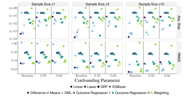
Panel B: Statistical Surrogacy

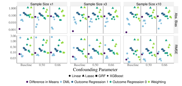
Notes: Figure 2 compares measurements of the absolute bias and root mean squared error for the estimators formulated in Section 4, in addition to the difference in means estimator defined in (5.1). The y-axes are displayed in logs, base 10. The long-term outcome is total household assets. Panels A and B display results for the Latent Unconfounded Treatment and Statistical Surrogacy Models defined in 2.1 and 2.2, respectively. The columns of each panel vary the sample size multiplier $h$. Each sub-panel displays results for the baseline, unconfounded, case, as well as for the cases that the confounding parameter $\phi$ has been set to $1/2$ and $2/3$. Results for each estimator are displayed with dots of different colors. Results for different nuisance parameter estimators are displayed with dots of different shapes.

In both the Latent Unconfounded Treatment Model and the Statistical Surrogacy Model, the biases of the DML estimators considered in Section 4.1 tend to be substantially smaller than the biases of the alternative outcome regression or weighting estimators considered in Section 4.2, so long as the nuisance parameters are not estimated by linear regression. The weighting estimator has performance more comparable to the DML estimator in the Latent Unconfounded Treatment Model. The performances of the weighting estimator and the outcome regression estimators in the Statistical Surrogacy Model are more similar.

Figure 3 displays measurements of estimator quality for just the DML estimators in a format analogous to Figure 2, with the addition of a third row measuring one minus the coverage probability of confidence intervals constructed around each estimator. We report these estimates of coverage probabilities in Supplementary Section D.5. Confidence intervals constructed with the intervals given in (A.41) around the estimators formulated in 4.1 have coverage probabilities that are reasonably close to the nominal level.

Figure 3. Finite-Sample Performance with Different Nuisance Parameter Estimators

Panel A: Latent Unconfounded Treatment

Panel B: Statistical Surrogacy

Notes: Figure 3 displays measurements of the quality of the estimators formulated in Section 4.1 implemented with several alternative choices of nuisance parameter estimators. The long-term outcome is total household assets. Panels A and B display results for the estimators defined in 4.1 for the Latent Unconfounded Treatment and Statistical Surrogacy Models defined in 2.1 and 2.2, respectively. The columns of each panel vary the sample size multiplier $h$. The rows of each panel display the absolute value of the bias, one minus the coverage probability, and the root mean squared error of each estimator, from top to bottom, respectively. A dotted line denoting one minus the nominal coverage probability, 0.05, is displayed in each sub-panel in the third row. Each sub-panel displays a bar graph comparing measurements of the performance of the estimator defined in 4.1, constructed with three types of nuisance parameter estimators, with the difference in means estimator (5.1). Each sub-panel displays results for the baseline, unconfounded, case, as well as for the cases that the confounding parameter $\phi$ has been set to $1/2$ and $2/3$.

6. Conclusion

We study the estimation of long-term treatment effects through the combination of short-term experimental and long-term observational data sets. We derive efficient influence functions and calculate corresponding semiparametric efficiency bounds for this problem. These calculations facilitate the development of estimators that accommodate the applications of standard machine learning algorithms for estimating nuisance parameters. We demonstrate with simulation that these estimators are able to recover long-term treatment effects in realistic settings.

Important unresolved practical issues remain. Methods for choosing valid and informative short-term outcomes and assessing of the sensitivity of estimates to violations of identifying assumptions would be valuable. Additional useful extensions include the incorporation of instruments and continuous treatments and the accommodation of settings with limited covariate overlap.

In the case of estimation of average treatment effects under unconfoundedness, recent promising work (e.g., Athey et al.,, 2018; Bradic et al.,, 2019; Tan,, 2020) has developed estimators that are specifically optimized to handle high-dimensional covariates and are able to attain various notions of optimality under weak assumptions on, e.g., the sparsity of the outcome regression or propensity score models. It is not immediately clear how to apply these ideas to long-term average treatment effects. Further consideration of this problem would be a potentially valuable extension, as the resultant estimators may be particularly well-suited to the case where there are many short-term outcomes. Some progress on a related problem (where, effectively, there is a single short-term outcome) has been made by Viviano and Bradic, (2021).

Supplemental Appendix to: Semiparametric Estimation of
Long-Term Treatment Effects Jiafeng Chen David M. Ritzwoller Harvard Business School Stanford Graduate School of Business jiafengchen@g.harvard.edu ritzwoll@stanford.edu

Contents  appendix.Asubsection.A.1subsection.A.2subsection.A.3subsection.A.4subsection.A.5subsection.A.6subsection.A.7subsection.A.8subsubsection.A.8.1subsubsection.A.8.2subsubsection.A.8.3appendix.Bsubsection.B.1subsection.B.2subsection.B.3appendix.Csubsection.C.1subsection.C.2subsubsection.C.2.1subsubsection.C.2.2subsubsection.C.2.3subsubsection.C.2.4subsubsection.C.2.5subsection.C.3subsubsection.C.3.1subsubsection.C.3.2subsubsection.C.3.3subsubsection.C.3.4appendix.Dsubsection.D.1subsection.D.2subsection.D.3subsection.D.4section*.52section*.53section*.54section*.55section*.56section*.57subsection.D.5  

Appendix A Proofs for Results Presented in the Main Text

A.1. Proof of Proposition 2.1

Unless otherwise noted, we drop the dependence on the individual $i$. It will suffice to consider the parameter

$$\theta_{1,1}=\mathbb{E}_{P_{\star}}[Y(1)\mid G=1]\leavevmode\nobreak\ ,$$

as the point-identification of $\theta_{1,0}=\mathbb{E}[Y(0)\mid G=1]$ will follow by an analogous argument.

We consider Latent Unconfounded Treatment Model, specified in 2.1, and repeat the argument provided in support of Theorem 1 of Athey et al., 2020a . Define the functions

$$\mu_{1}(s,x) =\mathbb{E}_{P}[Y\mid S=s,X=x,W=1,G=1]$$

$$=\mathbb{E}_{P_{\star}}[Y(1)\mid S(1)=s,X=x,W=1,G=1]$$

and

$$\overline{\mu}_{1}(x) =\mathbb{E}_{P}[\mu_{1}(S,X)\mid X=x,W=1,G=0]$$

$$=\mathbb{E}_{P_{\star}}[\mu_{1}(S(1),X)\mid X=x,W=1,G=0]$$

and observe that, by Assumption 2.2, $\mu_{1}(s,x)$ is identified from the observational sample and $\overline{\mu}_{1}(x)$ is identified from the experimental sample given the identification of $\mu_{1}(s,x)$. Observe that

$$\mathbb{E}_{P_{\star}}[Y(1)\mid G=1]$$

$$=\mathbb{E}_{P_{\star}}[\mathbb{E}_{P_{\star}}[Y(1)\mid X,G=1]\mid G=1]$$

$$=\mathbb{E}_{P_{\star}}[\mathbb{E}_{P_{\star}}[Y(1)\mid X,G=0]\mid G=1]$$ (Assumption 2.3)

$$=\mathbb{E}_{P_{\star}}[\mathbb{E}_{P_{\star}}[\mathbb{E}_{P_{\star}}[Y(1)\mid S(1),X,G=1]\mid X,G=0]\mid G=1]$$ (Assumption 2.3)

$$=\mathbb{E}_{P_{\star}}[\mathbb{E}_{P_{\star}}[\mathbb{E}_{P_{\star}}[Y(1)\mid S(1),X,W=1,G=1]\mid X,G=0]\mid G=1]$$ (Assumption 2.4)

$$=\mathbb{E}_{P_{\star}}[\mathbb{E}_{P_{\star}}[\mu_{1}(S(1),X)]\mid X,G=0]\mid G=1]$$

$$=\mathbb{E}_{P_{\star}}[\mathbb{E}_{P_{\star}}[\mu_{1}(S(1),X)]\mid X,W=1,G=0]\mid G=1]$$ (Assumption 2.1)

$$=\mathbb{E}_{P_{\star}}[\overline{\mu}_{1}(X)\mid G=1]\leavevmode\nobreak\ .$$

Hence, $\tau_{1}$ is identified as $\overline{\mu}_{1}(x)$ is identified.

A.2. Proof of Proposition 2.2

We consider the Statistical Surrogacy Model, specified in 2.2. Define the function

$$\nu(s,x)=\mathbb{E}_{P}[Y\mid S=s,X=x,G=1]$$

and observe that $\nu(s,x)$ is identified from the observational sample by Assumption 2.2. Observe that

$$\mathbb{E}_{P_{\star}}[Y(1)\mid G=1] =\mathbb{E}_{P_{\star}}[\mathbb{E}_{P_{\star}}[Y(1)\mid X,G=1]\mid G=1]$$

$$=\mathbb{E}_{P_{\star}}[\mathbb{E}_{P_{\star}}[Y(1)\mid X,G=0]\mid G=1]$$ (Assumption 2.3)

$$=\mathbb{E}_{P_{\star}}[\mathbb{E}_{P_{\star}}[Y(1)\mid X,W=1,G=0]\mid G=1]\leavevmode\nobreak\ ,$$ (Assumption 2.1)

and that

$$\mathbb{E}_{P_{\star}}[Y(1)\mid X,W=1,G=0]$$

$$=\mathbb{E}_{P}[Y\mid X,W=1,G=0]$$

$$=\mathbb{E}_{P}[\mathbb{E}_{P}[Y\mid S,X,W=1,G=0]\mid X,W=1,G=0]$$

$$=\mathbb{E}_{P}[\mathbb{E}_{P}[Y\mid S,X,G=0]\mid X,W=1,G=0]$$ (Assumption 2.5)

$$=\mathbb{E}_{P}[\mathbb{E}_{P}[Y\mid S,X,G=1]\mid X,W=1,G=0]$$ (Assumption 2.6)

$$=\mathbb{E}_{P}[\nu(S,X)\mid X,W=1,G=0]\leavevmode\nobreak\ .$$

It is clear that $\mathbb{E}_{P}[\nu(S,X)\mid X,W=1,G=0]$ is identified from the experimental sample by Assumption 2.2, and that therefore $\tau_{1}$ is identified.  

A.3. Proof of Theorem 3.1. Part 1

Throughout, for a general functional $\varphi$ on $\mathcal{M}_{\lambda}$ and an arbitrary random variable $D$ with distribution $Q$ in $\mathcal{M}_{\lambda}$, we write $\varphi(Q)=\varphi(D)$ with a minor abuse of notation.We let

$$\varphi^{\prime}(D)=\varphi^{\prime}(D;0)=\frac{d}{d\varepsilon}\varphi(Q_{\varepsilon}){\small\bigg{\rvert}}_{\varepsilon=0}$$

denote the pathwise derivative of $\varphi(\cdot)$ on some regular parametric submodel $\mathcal{Q}=\{Q_{\varepsilon}:\varepsilon\in[-1,1]\}$ of $\mathcal{M}_{\lambda}$ evaluated at $\varepsilon=0$.

It suffices to derive the efficient influence function for the parameter $\theta_{1,1}$, defined more generally by $\theta_{w,g}=\mathbb{E}[Y_{i}(w)\mid G_{i}=g]$, as an analogous argument will hold for $\theta_{0,1}$. Unless otherwise noted, we drop the dependence on the individual $i$. We omit the subscript $w$ on the nuisance functions $\mu_{w}(s,x)$, $\overline{\mu}_{w}(x)$, and $\varrho_{w}(s,x)$, as only the case $W=1$ will be relevant.

The presentation of the proof will be somewhat constructive, as we hope to convey the rationale behind the form of the efficient influence function, for which we have had to take a few educated guesses in forming a conjecture. Nonetheless, we state that the efficient influence function $\psi_{1,1}(b)$ takes the form

$$\psi_{1,1}(b)=\frac{gw(y-\mu(s,x))}{\pi\rho(s,x)}+\frac{(1-g)w}{(1-\gamma(x))\varrho(x)}\frac{\gamma(x)}{\pi}(\mu(s,x)-\overline{\mu}(x))+\frac{g}{\pi}(\overline{\mu}(x)-\theta_{1,1})$$

The reader can of course verify Theorem 3.1 directly by using this stated form of the influence function and checking a series of conditions that we lay out.

The argument proceeds as follows. First, we factorize the density of the observed data and relate each factor to conditional densities of the complete data distribution. Second, for an arbitrary smooth parametric submodel, we characterize the tangent space of the distribution of the observed data as a linear space of mean-zero square-integrable functions. Third, we conjecture a functional form that explicitly resides in the tangent space, where we note that the efficient influence function is the unique influence function for the target statistical functional $\theta_{1,1}$ in the tangent space of $\theta_{1,1}$ (Chapter 25 of Van der Vaart,, 1998). Fourth, we state the conditions an influence function of the pathwise derivative of $\theta_{1,1}$ necessarily satisfies, and we verify that the conjectured efficient influence function satisfies these conditions.

Density Factorization. Consider the random variable

$$A_{1}=(Y(1),S(1),W,G,X)\equiv(Y^{*},S^{*},W,G,X)$$

where we observe $B_{1}=(WGY^{*},WS^{*},W,G,X)$. Let $Y=WGY^{*}$ and $S=WS^{*}$. Recall that the distribution of the complete data is denoted by $P_{\star}$, with density $p_{\star}$ with respect to $\lambda$, and that the distribution of the observed data is denoted by $P$, with density $p$ with respect to $\lambda$. Observe that the densities under the complete data distribution and the observed data distribution agree when data isn’t missing. That is, for all $(y,s)\in\mathbb{R}\times\mathbb{R}^{d}$ and events $E\in\mathcal{A}$, we have that

$$p_{\star}(y\mid W=1,G=1,E)=p(y\mid W=1,G=1,E)$$

and

$$p_{\star}(s\mid W=1,E)=p(s\mid W=1,E)$$

and that for all events $E$ measurable with respect to the $\sigma$-algebra generated by $(W,G,X)$, we have that $P(E)=P_{\star}(E)$.

By Assumptions 2.1, 2.3, and 2.4, the density of the observed data $p$ admits the factorization

$$p(b_{1})=\,\, p(y\mid G=1,X=x,W=1,S=s)^{wg}p(s,W=1\mid G=1,X=x)^{wg}$$

$$p(s\mid G=0,X=x,W=1)^{w(1-g)}$$

$$P(W=w\mid G=0,X=x)^{1-g}P(W=0\mid G=1,X=x)^{(1-w)g}P(G=g\mid X=x)p(x)\leavevmode\nobreak\ .$$

Each of the terms of this expression can be rewritten in terms of the density of the complete data $p_{\star}$. In particular, we have that the first term can be written

$$p(y\mid G=1,X=x,W=1,S=s) =p_{\star}(y\mid G=1,X=x,W=1,S=s)$$

$$=p_{\star}(y\mid G=1,X=x,S=s)$$ (Assumption 2.4)

$$=p_{\star}(y\mid x,s)\leavevmode\nobreak\ , p_{\star}$$ (Assumption 2.3, noting that is the measure of the potential outcomes. )

the second and third terms can be written

$$p(s,W=1\mid G=1,X=x) =p_{\star}(S^{*}=s,W=1\mid G=1,X=x)$$

$$=p_{\star}(W=1\mid S^{*}=s,G=1,X=x)p_{\star}(S^{*}=s\mid G=1,X=x)$$

$$=\rho(s,x)p_{\star}(s\mid x)$$ (Assumption 2.3)

and

$$p(s\mid G=0,X=x,W=1) =p_{\star}(S^{*}=s\mid G=0,X=x)$$ (Assumption 2.1)

$$=p_{\star}(s\mid x)\leavevmode\nobreak\ ,$$ (Assumption 2.3)

the fourth term can be written

$$P(W=w\mid G=0,X=x) =\varrho(x)^{w}(1-\varrho(x))^{1-w}\leavevmode\nobreak\ ,$$ (Assumption 2.1)

and finally the fifth term can be written

$$P(W=0\mid G=1,X=x) =P_{\star}(W=0\mid G=1,X=x)$$

$$=\int P_{\star}(W=0\mid G=1,X=x,S=s)\,dP_{\star}(s\mid x)$$

$$=\int(1-\rho(s,x))p_{\star}(s\mid x)\,ds.$$

As a result, we obtain a factorization of the density of the observed data in terms of conditional distributions of the complete data

$$p(b_{1})=\,\, p_{\star}(y\mid x,s)^{wg}p_{\star}(s\mid x)^{w}\rho(s,x)^{wg}\left({\int(1-\rho(s,x))p_{\star}(s\mid x)\,ds}\right)^{(1-w)g}$$

$$\gamma(x)^{g}(1-\gamma(x))^{1-g}(\varrho(x)^{w}(1-\varrho(x))^{1-w})^{1-g}p(x)\leavevmode\nobreak\ .$$ (A.1)

Characterization of the Tangent Space. Let $\mathcal{P}$ be any regular parametric submodel of $\mathcal{M}_{\lambda}$ indexed by $\varepsilon\in\mathbb{R}$, with densities $p_{\varepsilon}:=dP_{\varepsilon}/d\lambda$ with $p_{0}=dP/d\lambda$ and such that Assumptions 2.1, 2.3, and 2.4 hold for each $P_{\varepsilon}\in\mathcal{P}$. Let the subscript _⋆ distinguish log densities of the complete data from log densities of the observed data. By the factorization (A.1), we obtain the score

$$\ell^{\prime}(b_{1}) =wg\cdot\ell^{\prime}_{*}(y\mid x,s)+w\cdot\ell^{\prime}_{*}(s\mid x)+\ell^{\prime}_{*}(g,x)$$

$$-g(1-w)\left(\frac{\mathbb{E}_{P_{\star}}[\rho(S^{*},X)\ell^{\prime}_{*}(S^{*}\mid X)\mid G=0,W=1,X=x]}{1-\mathbb{E}_{P_{\star}}[\rho(S^{*},X)\mid G=0,W=1,X=x]}\right)$$

$$+g\left(w\cdot\frac{\rho^{\prime}(s,x)}{\rho(s,x)}-(1-w)\frac{\mathbb{E}_{P_{\star}}[\rho^{\prime}(S^{*},X)\mid G=0,W=1,X=x]}{1-\mathbb{E}_{P_{\star}}[\rho(S^{*},X)\mid G=0,W=1,X=x]}\right)$$

$$+(1-g)\varrho^{\prime}(x)\left(\frac{w-\varrho(x)}{\varrho(x)(1-\varrho(x))}\right)\leavevmode\nobreak\ .$$ (A.2)

Thus, the tangent space $\mathcal{T}$ is given by mean-square closure of the linear span of the functions

$$s(b_{1}) =wg\cdot s_{1}(y\mid x,s)+w\cdot s_{2}(s\mid x)+s_{3}(g,x)$$

$$-g(1-w)\left(\frac{\mathbb{E}_{P_{\star}}[\rho(S^{*},X)s_{2}(S^{*}\mid X)\mid G=0,W=1,X=x]}{1-\mathbb{E}_{P_{\star}}[\rho(S^{*},X)\mid G=0,W=1,X=x]}\right)$$

$$+g\left(w\cdot\frac{s_{4}(s,x)}{\rho(s,x)}-(1-w)\frac{\mathbb{E}_{P_{\star}}[s_{4}(S^{*},X)\mid G=0,W=1,X=x]}{1-\mathbb{E}_{P_{\star}}[\rho(S^{*},X)\mid G=0,W=1,X=x]}\right)$$

$$+(1-g)\left(s_{5}(x)\frac{w-\varrho(x)}{\varrho(x)(1-\varrho(x))}\right)\leavevmode\nobreak\ ,$$

where the functions $s_{1}$ through $s_{5}$ range over the space of mean-zero and square integrable functions that satisfy the restrictions

$$\mathbb{E}_{P}[s_{1}(Y\mid S,X)\mid W=1,G=1,S,X]=\mathbb{E}_{P_{\star}}[s_{1}(Y^{*}\mid S^{*},X)\mid S^{*}=s,X=x] =0\leavevmode\nobreak\ ,$$

$$\mathbb{E}_{P}[s_{2}(S\mid X)\mid W=1,G=0,X]=\mathbb{E}_{P_{\star}}[s_{2}(S^{*}\mid X)\mid X=x] =0\leavevmode\nobreak\ \text{, and}$$

$$\mathbb{E}_{P}[s_{3}(G,X)] =0\leavevmode\nobreak\ .$$

Pathwise Differentiability Conditions. In the following calculations, it is often easier to work with the complete data distribution. To that end, we note that for an arbitrary measurable function $h$, we have that certain conditional means of the observed distribution equal certain conditional means of the complete data distribution:

$$\mathbb{E}_{P}[h(Y,S,X)\mid W=1,G=1,X=x,S=s] =\mathbb{E}_{P_{\star}}[h(Y^{*},S,X)\mid G=1,X=x,S^{*}=s]\leavevmode\nobreak\ ,$$

$$\mathbb{E}_{P}[h(S,X)\mid G=0,W=1,X=x] =\mathbb{E}_{P_{\star}}[h(S^{*},X)\mid G=0,X=x]$$

$$=\mathbb{E}_{P_{\star}}[h(S^{*},X)\mid G=1,X=x]\leavevmode\nobreak\ ,$$

$$\mathbb{E}_{P}[h(X)\mid G=1] =\mathbb{E}_{P_{\star}}\left[{h(X)\mid G=1}\right]\leavevmode\nobreak\ ,$$

and, as a result, for $h$,

$$\mathbb{E}_{P}[\mathbb{E}_{P}[\mathbb{E}_{P}[h(Y,S,X)\mid W=1,G=1,X,S]\mid W=1,G=0,X]\mid G=1]$$

$$\quad=\mathbb{E}_{P_{\star}}\left[{h(Y^{*},S^{*},X)\mid G=1}\right]=\mathbb{E}_{P_{\star}}\left[{\frac{G}{\pi}h(Y^{*},S^{*},X)}\right]\leavevmode\nobreak\ .$$

Note that $\theta_{1,1}$ is such a functional with $h(y,s,x)=y$.

Observe that the parameter of interest can be written

$$\theta_{1,1} =\mathbb{E}_{P_{\star}}[Y^{*}\mid G=1]$$

$$=\mathbb{E}_{P}[\mathbb{E}_{P}[\mathbb{E}_{P}[Y\mid W=1,G=1,X,S]\mid W=1,G=0,X]\mid G=1]$$

$$=\iiint\frac{y}{\pi}p_{\star}(y\mid s,x)p_{\star}(s\mid x)p(x,G=1)\,\text{d}\lambda(y)\text{d}\lambda(s)\text{d}\lambda(x)\leavevmode\nobreak\ .$$

The pathwise derivative of this parameter at 0 on $\mathcal{P}$ is given by

$$\theta_{1,1}^{\prime} =\mathbb{E}_{P_{\star}}[Y^{*}\ell^{\prime}(Y^{*}\mid S^{*},X)\mid G=1]$$

$$+\mathbb{E}_{P_{\star}}[Y^{*}\ell^{\prime}(S^{*}\mid X)\mid G=1]+\mathbb{E}_{P_{\star}}[Y^{*}\ell^{\prime}(X,G=1)\mid G=1]\leavevmode\nobreak\ .$$ (A.3)

Now, observe that

$$G\cdot\ell^{\prime}_{*}(X,G=1) =G\cdot\ell^{\prime}_{*}(X,G)-G\cdot\ell^{\prime}_{*}(G=1)\leavevmode\nobreak\ ,$$

and that

$$\ell^{\prime}_{*}(G=1) =\mathbb{E}_{P_{\star}}[\ell^{\prime}_{*}(X,G)\mid G=1]\leavevmode\nobreak\ .$$

Thus, each of the terms in (A.3) can be written in terms of conditional scores by

$$\mathbb{E}_{P_{\star}}[Y^{*}\ell^{\prime}(Y^{*}\mid S^{*},X)\mid G=1] =\mathbb{E}_{P_{\star}}[\pi^{-1}GY^{*}\ell^{\prime}_{*}(Y^{*}\mid S^{*},X)]\leavevmode\nobreak\ ,$$

$$\mathbb{E}_{P_{\star}}[Y^{*}\ell^{\prime}(S^{*}\mid X)\mid G=1] =\mathbb{E}_{P_{\star}}[\pi^{-1}GY^{*}\ell^{\prime}_{*}(S^{*}\mid X)]\leavevmode\nobreak\ \text{, and}$$

$$\mathbb{E}_{P_{\star}}[Y^{*}\ell^{\prime}(X,G=1)\mid G=1] =\mathbb{E}_{P_{\star}}[\pi^{-1}GY^{*}\ell^{\prime}_{*}(X,G=1)]$$

$$=\mathbb{E}_{P_{\star}}[\pi^{-1}GY^{*}\ell^{\prime}_{*}(X,G)]-\mathbb{E}_{P_{\star}}[\pi^{-1}GY^{*}]\ell^{\prime}_{*}(G=1)$$

$$=\mathbb{E}_{P_{\star}}[\pi^{-1}GY^{*}\ell^{\prime}_{*}(X,G)]-\theta_{1,1}\cdot\mathbb{E}_{P_{\star}}[\ell^{\prime}_{*}(X,G)\mid G=1]\leavevmode\nobreak\ ,$$

respectively.

An influence function for $\theta_{1,1}$ is a mean-zero and square-integrable function $\tilde{\psi}_{1,1}(B_{1})$ that satisfies the condition

$$\theta_{1,1}^{\prime}=\mathbb{E}_{P}[\tilde{\psi}_{1,1}(B_{1})\ell^{\prime}(B_{1})]\leavevmode\nobreak\ .$$ (A.4)

Hence, by (A.2) and (A.3), in order to establish that a mean-zero and square-integrable function $\tilde{\psi}_{1,1}(B_{1})$ is an influence function for $\theta_{1,1}$, it suffices to show that the terms in the right-hand side of (A.4) match the terms in the right-hand side of (A.3):

$$\frac{1}{\pi}\mathbb{E}_{P_{\star}}[GY^{*}\ell^{\prime}_{*}(Y^{*}\mid S^{*},X)] =\mathbb{E}_{P}\left[{\tilde{\psi}_{1,1}(B_{1})GW\ell^{\prime}_{*}(Y\mid S,X)}\right]\leavevmode\nobreak\ ,$$ (A.5)

$$\frac{1}{\pi}\mathbb{E}_{P_{\star}}[GY^{*}\ell^{\prime}_{*}(S^{*}\mid X)] =\mathbb{E}_{P}\Bigg{[}\tilde{\psi}_{1,1}(B_{1})\Bigg{(}W\ell^{\prime}_{*}(S\mid X)$$

$$\quad\quad\quad\quad-G(1-W)\frac{\int\rho(s,X)p^{\prime}_{*}(s\mid X)\,\text{d}\lambda(s)}{1-\int\rho(s,X)p_{\star}(s\mid X)\,\text{d}\lambda(s)}\Bigg{)}\Bigg{]}\leavevmode\nobreak\ ,$$ (A.6)

$$\mathbb{E}_{P}[\tilde{\psi}_{1,1}(B_{1})\ell^{\prime}_{*}(G,X)] =\frac{1}{\pi}\mathbb{E}_{P_{\star}}[GY^{*}\ell^{\prime}_{*}(G,X)]-\theta_{1,1}\cdot\mathbb{E}_{P_{\star}}[\ell^{\prime}_{*}(G,X)\mid G=1]\leavevmode\nobreak\ ,$$ (A.7)

$$0 =\mathbb{E}_{P}\Bigg{[}\tilde{\psi}_{1,1}(B_{1})G\Bigg{(}W\frac{\rho^{\prime}(S,X)}{\rho(S,X)}$$

$$\quad\quad\quad\quad-(1-W)\frac{\int\rho^{\prime}(s,X)p_{\star}(s\mid X)\text{d}\lambda(s)}{1-\int\rho(s,X)p_{\star}(s\mid X)\,\text{d}\lambda(s)}\Bigg{)}\Bigg{]}\leavevmode\nobreak\ ,$$ (A.8)

$$0 =\mathbb{E}_{P}\left[{\tilde{\psi}_{1,1}(B_{1})(1-G)\frac{W-\varrho(X)}{\varrho(X)(1-\varrho(X))}\varrho^{\prime}(X)}\right]\leavevmode\nobreak\ .$$ (A.9)

Conjectured Efficient Influence Function. We begin by considering an element of the tangent space. For the unspecified functions $a(s,x)$ and $b(x)$, consider the choices

$$s_{1}(y,s,x) =\frac{y-\mu(s,x)}{\pi\rho(s,x)}\leavevmode\nobreak\ , s_{2}(s,x) =\frac{1}{\varrho(x)}\frac{a(s,x)}{(1-\gamma(x))}\leavevmode\nobreak\ ,$$

$$s_{3}(g,x) =g\cdot b(x), s_{4}(s,x) =-\rho(s,x)s_{2}(s,x)\leavevmode\nobreak\ \text{, and}$$

$$s_{5}(x) =0\leavevmode\nobreak\ .$$ (A.10)

These choices correspond to the following conjectured efficient influence function

$$\psi_{1,1}(b_{1}) =gw\cdot s_{1}(y,s,x)+w\cdot s_{2}(s,x)-gw\cdot s_{2}(s,x)+gb(x)$$

$$=gw\cdot s_{1}(y,s,x)+(1-g)w\cdot s_{2}(s,x)+g\cdot b(x)$$

$$=\frac{gw(y-\mu(s,x))}{\pi\rho(s,x)}+\frac{(1-g)w}{(1-\gamma(x))\varrho(x)}a(s,x)+g\cdot b(x)\leavevmode\nobreak\ .$$ (A.11)

In particular, $s_{4}$ is chosen so that certain terms cancel to construct the term $(1-g)ws_{2}(s,x)$, which does not, prima facie, belong in the tangent space (A.2).

In order to ensure that $\psi_{1,1}(b_{1})$ belongs to the tangent space, we require

$$\mathbb{E}_{P}[a(S,X)\mid W=1,G=0,X=x] =\mathbb{E}_{P_{\star}}[a(S^{*},X)\mid X=x]=0\leavevmode\nobreak\ \text{, and}$$ (A.12)

$$\mathbb{E}_{P}[G\cdot b(X)] =0\leavevmode\nobreak\ .$$ (A.13)

In the sequel, we verify that the choices

$$a(s,x) =\frac{\gamma(x)}{\pi}(\mu(s,x)-\overline{\mu}(x))\leavevmode\nobreak\ \text{, and}$$

$$b(x) =\frac{\overline{\mu}(x)-\theta_{1,1}}{\pi}$$

satisfy these conditions, and, moreover, give rise to the efficient influence function by satisfying the conditions (A.5)–(A.9).

Verifying Pathwise Differentiability Conditions. We begin by stating and proving a useful lemma for handling terms of the form $GWh(Y,S,X)$.

Lemma A.1.

Under the assumptions of Theorem 3.1, if $h(y,s,x)$ is any measurable function, then

$$\mathbb{E}_{P}\left[{\frac{GW}{\rho(S,X)}h(Y,S,X)}\right]=\mathbb{E}_{P_{\star}}\left[{Gh(Y^{*},S^{*},X)}\right]=\mathbb{E}_{P_{\star}}\left[{G\mathbb{E}[h(Y^{*},S^{*},X)\mid S^{*},X]}\right]\leavevmode\nobreak\ .$$

Proof.

Observe that

$$\mathbb{E}_{P}\left[{\frac{GW}{\rho(S,X)}h(Y,S,X)}\right] =\mathbb{E}_{P}\left[{\pi\frac{W}{\rho(S,X)}h(Y,S,X)\mid G=1}\right]$$

$$=\pi\mathbb{E}_{P_{\star}}\left[{\frac{W}{\rho(S^{*},X)}h(Y^{*},S^{*},X)\mid G=1}\right]$$

$$=\pi\mathbb{E}_{P_{\star}}\bigg{[}\rho^{-1}(S^{*},X)\mathbb{E}_{P_{\star}}[W\mid S^{*},X,G=1]$$

$$\quad\quad\quad\mathbb{E}_{P_{\star}}[h(Y^{*},S^{*},X)\mid S^{*},X,G=1]\mid G=1\bigg{]}$$ (Assumption 2.4)

$$=\mathbb{E}_{P_{\star}}[\pi h(Y^{*},S^{*},X)\mid G=1]$$

$$=\mathbb{E}_{P_{\star}}[Gh(Y^{*},S^{*},X)]\leavevmode\nobreak\ ,$$

giving the first equality. The second equality then follows from

$$\mathbb{E}_{P_{\star}}[Gh(Y^{*},S^{*},X)] =\pi\mathbb{E}_{P_{\star}}[\mathbb{E}_{P_{\star}}[h(Y^{*},S^{*},X)\mid S^{*},X,G=1]\mid G=1]$$

$$=\mathbb{E}_{P_{\star}}[G\mathbb{E}_{P_{\star}}[h(Y^{*},S^{*},X)\mid S^{*},X,G=1]]$$

$$=\mathbb{E}_{P_{\star}}[G\mathbb{E}_{P_{\star}}[h(Y^{*},S^{*},X)\mid S^{*},X]]\leavevmode\nobreak\ ,$$

completing the proof.  

It now suffices to verify the conditions (A.5)–(A.9) for choices of $a(S,X)$ and $b(X)$ that satisfy (A.12) and (A.13). The remainder of the proof verifies these conditions sequentially.

Condition (A.5): Observe that

$$\mathbb{E}_{P}\left[{\psi_{1,1}(B_{1})GW\ell^{\prime}_{*}(Y\mid S,X)}\right] =\mathbb{E}_{P}\left[{\frac{GWY}{\pi\rho(S,X)}\ell^{\prime}_{*}(Y\mid S,X)}\right]$$

$$=\mathbb{E}_{P_{\star}}\left[{\pi^{-1}GY^{*}\ell^{\prime}_{*}(Y^{*}\mid S^{*},X)}\right]\leavevmode\nobreak\ ,$$ (Lemma A.1)

as required.

Condition (A.6): We derive the restrictions on $a(s,x)$ implied by (A.6). Observe that the inner product from (A.6) can be written

$$\mathbb{E}_{P}\left[{\psi_{1,1}(B_{1})\left({W\ell^{\prime}_{*}(S\mid X)-G(1-W)\frac{\mathbb{E}_{P_{\star}}[\rho(S,X)\ell^{\prime}_{*}(S\mid X)\mid X]}{1-\mathbb{E}_{P_{\star}}[\rho(S,X)\mid X]}}\right)}\right]$$

$$\quad=\mathbb{E}_{P}\left[{\frac{GW(Y-\mu(S,X))\ell^{\prime}_{*}(S\mid X)}{\pi\rho(S,X)}}\right]-\mathbb{E}_{P}\left[{\frac{b(X)G(1-W)\mathbb{E}_{P_{\star}}[\rho(S,X)\ell^{\prime}_{*}(S\mid X)\mid X]}{1-\mathbb{E}_{P_{\star}}[\rho(S,X)\mid X]}}\right]$$

$$\quad+\mathbb{E}_{P}\left[{\frac{(1-G)Wa(S,X)}{(1-\gamma(X))\varrho(X)}\ell^{\prime}_{*}(S\mid X)}\right]+\mathbb{E}_{P}\left[{GWb(X)\ell^{\prime}_{*}(S\mid X)}\right]\leavevmode\nobreak\ .$$

Note that the first term can be eliminated by Lemma A.1:

$$\mathbb{E}_{P}\left[{\frac{GW(Y-\mu(S,X))\ell^{\prime}_{*}(S\mid X)}{\pi\rho(S,X)}}\right] =0\leavevmode\nobreak\ .$$

Observe that

$$\mathbb{E}_{P_{\star}}[G(1-W)\mid X]=P_{\star}(W\mid G=1,X)\gamma(X)=(1-\mathbb{E}_{P_{\star}}[\rho(S,X)\mid X])\gamma(X),$$

and thus the second term is given by

$$\mathbb{E}_{P}\left[{\frac{b(X)G(1-W)\mathbb{E}_{P_{\star}}[\rho(S^{*},X)\ell^{\prime}_{*}(S^{*}\mid X)\mid X]}{1-\mathbb{E}_{P_{\star}}[\rho(S^{*},X)\mid X]}}\right]$$

$$\quad=\mathbb{E}_{P_{\star}}\left[{\gamma(X)b(X)\mathbb{E}_{P_{\star}}[\rho(S^{*},X)\ell^{\prime}_{*}(S^{*}\mid X)\mid X]}\right]$$

$$\quad=\mathbb{E}_{P_{\star}}[\gamma(X)b(X)\rho(S^{*},X)\ell^{\prime}_{*}(S^{*}\mid X)]\leavevmode\nobreak\ .$$

Next, observe that

$$\mathbb{E}_{P_{\star}}[(1-G)W\mid S^{*},X]=(1-\gamma(X))P_{\star}(W=1\mid G=0,S^{*},X)=(1-\gamma(X))\varrho(X),$$

and therefore the third term can be written

$$\mathbb{E}_{P}\left[{\frac{(1-G)W}{(1-\gamma(X))\varrho(x)}a(S,X)\ell^{\prime}_{*}(S\mid X)}\right]=\mathbb{E}_{P_{\star}}\left[{a(S^{*},X)\ell^{\prime}_{*}(S^{*}\mid X)}\right]\leavevmode\nobreak\ .$$

The fourth term is given by

$$\mathbb{E}_{P}[GWb(X)\ell^{\prime}_{*}(S\mid X)]=\mathbb{E}_{P_{\star}}[\gamma(X)q(S^{*},X)b(X)\ell^{\prime}_{*}(S\mid X)]\leavevmode\nobreak\ ,$$

which cancels with the second term.

Thus, the condition (A.6) is equivalent to

$$\mathbb{E}_{P_{\star}}[\ell^{\prime}_{*}(S^{*}\mid X)a(S^{*},X)]=\mathbb{E}_{P_{\star}}\left[{\pi^{-1}GY^{*}\ell^{\prime}_{*}(S^{*}\mid X))}\right].$$ (A.14)

We proceed by verifying this condition for a choice of $a(S,X)$ that satisfies (A.12), as required. Consider the function

$$a(s,x)=\frac{\gamma(x)}{\pi}(\mu(s,x)-\overline{\mu}(x))\leavevmode\nobreak\ .$$

Then $\mathbb{E}_{P_{\star}}[a(S^{*},X)\mid X]=0$, which satisfies (A.12). Moreover,

$$\mathbb{E}_{P_{\star}}[a(S^{*},X)\ell^{\prime}_{*}(S^{*}\mid X)] =\mathbb{E}_{P_{\star}}\left[{\frac{\gamma(X)}{\pi}\mu(S^{*},X)\ell^{\prime}_{*}(S^{*}\mid X)}\right]$$

$$=\mathbb{E}_{P_{\star}}\left[{\frac{\mathbb{E}_{P_{\star}}[G\mid S^{*},X]}{\pi}\mathbb{E}_{P_{\star}}\left[{Y^{*}\ell^{\prime}_{*}(S^{*}\mid X)\mid S^{*},X}\right]}\right]$$

$$=\mathbb{E}_{P_{\star}}\left[{\pi^{-1}GY^{*}\ell_{*}^{\prime}(S^{*}\mid X)}\right]\leavevmode\nobreak\ ,$$

where the second to last equality follows by Assumption 2.3, which verifies (A.14) and thereby (A.6).

Condition (A.7): We derive the restrictions on $b(x)$ implied by (A.7). Note that the conjectured influence function (A.11) can be written as

$$\psi(b_{1})=gw\cdot\alpha(y,s,x)+(1-g)w\cdot\beta(s,x)+gb(x),$$

where

$$\mathbb{E}_{P}[\alpha(Y,S,X)\mid S=s,X=x,G=1,W=1] =\mathbb{E}_{P}[\beta(S,X)\mid G=0,W=1,X=x]=0\leavevmode\nobreak\ .$$

We first show that the terms in (A.7) involving $\alpha$ and $\beta$ are zero. Indeed, for terms involving $\alpha$, we have that

$$\mathbb{E}_{P}[GW\cdot\alpha(Y,S,X)\ell^{\prime}_{*}(G,X)]=\pi\mathbb{E}_{P}[\alpha(Y,S,X)\ell^{\prime}_{*}(G,X)\mid G=1,W=1]P(W=1\mid G=1)=0$$

since $\mathbb{E}_{P}[\alpha(Y,S,X)\ell^{\prime}_{*}(G,X;0)\mid G=1,W=1]=0$. Analogously, we have that

$$\mathbb{E}_{P}[(1-G)W\beta(S,X)\ell^{\prime}_{*}(G,X;0)]=0.$$

Therefore, (A.7) is equivalent to

$$\frac{1}{\pi}\mathbb{E}_{P_{\star}}[GY^{*}\ell^{\prime}_{*}(G,X)]-\theta_{1,1}\mathbb{E}[\ell^{\prime}_{*}(G,X)\mid G=1]=\mathbb{E}_{P}[Gb(X)\ell^{\prime}_{*}(G,X)].$$ (A.15)

We proceed by verifying this condition for a choice of $b(X)$.

Consider the function

$$b(x)=\frac{1}{\pi}(\overline{\mu}(x)-\theta_{1,1})\leavevmode\nobreak\ ,$$

which satisfies (A.13). We can compute

$$\mathbb{E}_{P}[G\pi^{-1}\mu(X)\ell^{\prime}_{*}(G,X)] =\mathbb{E}_{P_{\star}}\left[{\frac{G}{\pi}\mathbb{E}_{P_{\star}}[\mu(S^{*},X)\mid G=0,W=1,X]\ell^{\prime}_{*}(G,X;0)]}\right]$$

$$=\mathbb{E}_{P_{\star}}\left[{\frac{G}{\pi}\ell^{\prime}_{*}(G,X;0)\mathbb{E}_{P_{\star}}[\mathbb{E}_{P_{\star}}[Y\mid W=1,G=1,S^{*},X]\mid X]}\right]$$

$$=\mathbb{E}_{P_{\star}}\left[{\frac{\gamma(X)}{\pi}\ell^{\prime}_{*}(G,X;0)\mathbb{E}_{P_{\star}}\left[{\mathbb{E}_{P_{\star}}\left[{Y^{*}\mid S^{*},X}\right]\mid X}\right]}\right]$$

$$=\mathbb{E}_{P_{\star}}\left[{\frac{\gamma(X)}{\pi}\ell^{\prime}_{*}(G,X;0)Y^{*}}\right]$$

$$=\mathbb{E}_{P_{\star}}\left[{\frac{\mathbb{E}_{P_{\star}}[G\mid Y^{*},X]}{\pi}\ell^{\prime}_{*}(G,X;0)Y^{*}}\right]$$

$$=\mathbb{E}_{P_{\star}}\left[{\frac{G}{\pi}Y^{*}\ell^{\prime}_{*}(G,X;0)}\right],$$

and

$$-\mathbb{E}_{P_{\star}}[G\pi^{-1}\theta_{1,1}\ell^{\prime}_{*}(G,X;0)]=-\theta_{1,1}\mathbb{E}_{P_{\star}}[\ell^{\prime}_{*}(1,X;0)\mid G=1]$$

which verifies (A.15) and thereby (A.7).

Condition (A.8): Since the first and second terms $\alpha(Y,S,X)$ and $\beta(S,X)$ in the conjectured efficient influence function (A.11) are mean zero conditional on $S^{*}$ and $X$ and $X$, respectively, the right-hand side of (A.8) is equal to

$$\mathbb{E}_{P}\left[{b(X)\left({GW\frac{\rho^{\prime}(S,X)}{\rho(S,X)}-G(1-W)\frac{\mathbb{E}_{P_{\star}}[\rho^{\prime}(S^{*},X)\mid X]}{1-\mathbb{E}_{P_{\star}}[\rho(S^{*},X)\mid X]}}\right)}\right]$$

$$=\mathbb{E}_{P_{\star}}\left[{b(X)\gamma(X)\mathbb{E}_{P_{\star}}\left[{\rho(S^{*},X)\frac{\rho^{\prime}(S^{*},X)}{\rho(S^{*},X)}-(1-\rho(S^{*},X))\frac{\mathbb{E}_{P_{\star}}[\rho^{\prime}(S^{*},X)\mid X]}{1-\mathbb{E}_{P_{\star}}[\rho(S^{*},X)\mid X]}\mid G=1,S^{*},X}\right]}\right]$$

$$=\mathbb{E}_{P_{\star}}\left[{b(X)\gamma(X)\left({\rho^{\prime}(S^{*},X)-(1-\rho(S^{*},X))\frac{\mathbb{E}_{P_{\star}}[\rho^{\prime}(S^{*},X)\mid X]}{1-\mathbb{E}_{P_{\star}}[\rho(S^{*},X)\mid X]}}\right)}\right]=0$$

by iterated expectation conditional on $X$.

Condition (A.9): The only term on the right-hand side of (A.9) is

$$\mathbb{E}_{P}[(1-G)W\cdot\beta(S,X)\cdot(W-\rho(X))\delta(X)]$$

for some function $\delta(\cdot)$, where $(1-G)W\cdot\beta(S,X)$ is the second term in the conjectured efficient influence function (A.11). We have:

$$\mathbb{E}_{P}[(1-G)W\cdot\beta(S,X)\cdot(W-\varrho(X))\cdot\delta(X)]$$

$$=\mathbb{E}_{P}[\mathbb{E}_{P}[W\cdot\beta(S,X)\cdot(W-\varrho(X))\cdot\delta(X)\mid G=0,X](1-\gamma(X))]$$

$$=\mathbb{E}_{P_{\star}}[\beta(S^{*},X)\varrho(X)(1-\varrho(X))\cdot\delta(X)]=0$$

by the condition $\mathbb{E}_{P_{\star}}[\beta(S^{*},X)\mid X]=0$, completing the proof.  

A.4. Proof of Theorem 3.1. Part 2

We maintain the notation of the proof of Theorem 3.1, Part 1. In particular, we omit the $w$ subscript in the nuisance function $\overline{\nu}_{w}(x)$ and let

$$A_{1}=(Y(1),S(1),W,G,X)=(Y^{*},S^{*},W,G,X)$$

and $B_{1}=(Y,S,W,G,X)$ denote the complete and observed data, respectively. The efficient influence function we construct is

$$\xi_{1,1}(b) =\frac{g}{\pi}\left(\frac{\gamma(x)}{\gamma(s,x)}\frac{1-\gamma(s,x)}{1-\gamma(x)}\frac{\varrho(s,x)(y-\nu(S,X))}{\varrho(x)}+(\overline{\nu}_{1}(x)-\theta_{1,1})\right)$$

$$+\frac{1-g}{\pi}\frac{\gamma(x)}{1-\gamma(x)}\left(\frac{w(\nu(S,X)-\overline{\nu}_{1}(x))}{\varrho(x)}\right)\leavevmode\nobreak\ .$$

Density Factorization. By Assumptions 2.1, 2.6, 2.3, and 2.5, the density $p$ of the observed data distribution admits the factorization

$$p(b_{1})=\,\, p(x)\gamma(x)^{g}(1-\gamma(x))^{1-g}$$

$$p(y\mid G=1,s,x)^{g}p(s\mid G=1,x)^{g}$$

$$p(s\mid G=0,W=1,x)^{w(1-g)}(\varrho(x)^{w}(1-\varrho(x))^{1-w})^{1-g}\leavevmode\nobreak\ .$$ (A.16)

Characterization of the Tangent Space. Let $\mathcal{P}$ be any regular parametric submodel of $\mathcal{M}_{\lambda}$ indexed by $\varepsilon\in\mathbb{R}$, with densities $p_{\varepsilon}:=dP_{\varepsilon}/d\lambda$ with $p_{0}=dP/d\lambda$ and such that Assumptions 2.1, 2.6, 2.3, and 2.5 hold for each $P_{\varepsilon}\in\mathcal{P}$. By the factorization (A.4), we obtain the score

$$\ell^{\prime}(b_{1})=\,\, g\ell^{\prime}(y\mid s,x,G=1)+g\ell^{\prime}(s\mid x,G=1)+w(1-g)\ell^{\prime}(s\mid W=1,x,G=0)+\ell^{\prime}(x)$$

$$+ \frac{g-\gamma(x)}{\gamma(x)(1-\gamma(x))}\gamma^{\prime}(x)+(1-g)\frac{w-\varrho(x)}{\varrho(x)(1-\varrho(x))}\varrho^{\prime}(x).$$ (A.17)

Thus, the tangent space $\mathcal{T}$ is given by the mean-square closure of the linear span of the functions

$$s(b_{1})=\,\, g\cdot s_{1}(y\mid s,x,G=1)+g\cdot s_{2}(s\mid x,G=1)+w(1-g)\cdot s_{3}(s\mid W=1,x,G=0)+s_{4}(x)$$

$$+ \frac{g-\gamma(x)}{\gamma(x)(1-\gamma(x))}s_{5}(x)+(1-g)\frac{w-\varrho(x)}{\varrho(x)(1-\varrho(x))}s_{6}(x)\leavevmode\nobreak\ ,$$ (A.18)

where the functions $s_{1}$ through $s_{6}$ range over the space of mean-zero and square integrable functions that satisfy the restrictions

$$0 =\mathbb{E}_{P}[s_{1}(Y\mid S,X,G=1)\mid S,X,G=1]$$

$$=\mathbb{E}_{P}[s_{1}(Y\mid S,X,G=1)\mid S,X]\leavevmode\nobreak\ ,$$ (A.19)

$$0 =\mathbb{E}_{P}[s_{2}(S\mid X,G=1)\mid X,G=1]\leavevmode\nobreak\ ,$$ (A.20)

$$0 =\mathbb{E}_{P}[s_{3}(S\mid W=1,X,G=0)\mid W=1,X,G=0]$$

$$=\mathbb{E}_{P_{\star}}[s_{3}(S^{*}\mid W=1,X,G=0)\mid X,G=0]\leavevmode\nobreak\ ,$$ (A.21)

$$0 =\mathbb{E}_{P}[s_{4}(X)]\leavevmode\nobreak\ ,$$ (A.22)

and $s_{5},$ and $s_{6}$ are unconstrained, where (A.19) and (A.21) follow from Assumption 2.6 and Assumption 2.1, respectively.

Pathwise Differentiability Representation. Recall from the proof of Proposition 2.1 that, by Assumptions 2.1, 2.6, 2.3, and 2.5, the target parameter $\theta_{1,1}$ can be written as

$$\theta_{1,1} =\mathbb{E}_{P_{\star}}[Y^{*}\mid G=1]$$

$$=\mathbb{E}_{P}\left[{\mathbb{E}_{P}\left[{\mathbb{E}_{P}[Y\mid S,X,G=1]\mid W=1,X,G=0}\right]\mid G=1}\right]$$

$$=\iiint yp(y\mid s,x,G=1)p(s\mid x,W=1,G=0)p(x\mid G=1)\,d\lambda(y)\,\,d\lambda(s)\,\,d\lambda(x)\leavevmode\nobreak\ .$$

The pathwise derivative of this parameter is given by

$$\theta_{1,1}^{\prime}=\mathbb{E}_{P}[\mathbb{E}_{P}[\mathbb{E}_{P}[YU(Y,S,X)\mid S,X,G=1]\mid X,W=1,G=0]\mid G=1]$$

with

$$U(y,s,x) =\ell^{\prime}(y\mid s,x,G=1)+\ell^{\prime}(s\mid x,W=1,G=0)+\ell^{\prime}(x\mid G=1)$$

$$=\ell^{\prime}(y\mid s,x,G=1)+\ell^{\prime}(s\mid x,W=1,G=0)$$

$$+\ell^{\prime}(x)+\frac{\gamma^{\prime}(x)}{\gamma(x)}-\frac{\mathbb{E}_{P}[\gamma^{\prime}(X)+\gamma(X)\ell^{\prime}(X)]}{\pi}\leavevmode\nobreak\ ,$$

where final three terms follow from

$$p^{\prime}(x\mid G=1)=\ell^{\prime}(x\mid G=1)p(x\mid G=1)$$

and Bayes’ rule in the form of

$$\ell(x\mid G=1)=\log\gamma(x)+\ell(x)-\log\int\gamma(x)p(x)\,d\lambda(x)\leavevmode\nobreak\ .$$

Observe that, using the definitions of $\nu(s,x)$ and $\overline{\nu}(x)$, we may further simplify the pathwise derivative to give

$$\theta_{1,1}^{\prime}=\,\, \mathbb{E}_{P}[\mathbb{E}_{P}[\mathbb{E}_{P}[Y\ell^{\prime}(Y\mid S,X,G=1)\mid S,X,G=1]\mid X,W=1,G=0]\mid G=1]$$

$$+\mathbb{E}_{P}[\mathbb{E}_{P}[\nu(S,X)\ell^{\prime}(S\mid X,G=0,W=1)\mid X,W=1,G=0]\mid G=1]$$

$$+\pi^{-1}\mathbb{E}_{P}\left[{\overline{\nu}(X)\left({\gamma^{\prime}(X)+\gamma(X)\ell^{\prime}(X)}\right)}\right]-\pi^{-1}\mathbb{E}_{P}[\gamma^{\prime}(X)+\gamma(X)\ell^{\prime}(X)]\theta_{1,1}.$$ (A.23)

An influence function for $\theta_{1,1}$ is a mean-zero and square-integrable function $\tilde{\xi}_{1,1}(B_{1})$ that satisfies the condition

$$\theta^{\prime}_{1,1}=\mathbb{E}[\tilde{\xi}(B_{1})\ell^{\prime}(B_{1})]\leavevmode\nobreak\ .$$ (A.24)

We make a conjecture for such a function and verify that it satisfies this condition and is an element of the tangent space $\mathcal{T}$, establishing that it is the efficient influence function.

Conjectured Efficient Influence Function. We conjecture that the efficient influence function takes the form

$$\xi_{1,1}(b_{1})=g(y-\nu(s,x))\cdot f_{1}(s,x)+w(1-g)(\nu(s,x)-\overline{\nu}(x))\cdot f_{2}(x)+g\cdot f_{3}(x)\leavevmode\nobreak\ ,$$ (A.25)

for functions $f_{1}(s,x)$, $f_{2}(x)$, and $f_{3}(x)$ to be specified, where $f_{3}$ will be chosen to satisfy

$$\mathbb{E}_{P}[f_{3}(X)\mid G=1]=0=\mathbb{E}_{P}[f_{3}(X)\gamma(X)]\leavevmode\nobreak\ .$$ (A.26)

Observe that for this choice, $\xi_{1,1}(b)$ will be an element of the tangent space $\mathcal{T}$. This follows as

$$s_{1}(y\mid s,x,G=1)=(y-\nu(s,x))f_{1}(s,x)$$

satisfies (A.19), we make the choice

$$s_{2}(s\mid X,G=1)=0$$

satisfying (A.20),

$$s_{3}(s\mid W=1,x,G=0)=(\nu(s,x)-\overline{\nu}(x))f_{2}(x)$$

satisfies (A.21), and that setting $s_{4}(x)=\gamma(x)f_{3}(x)$ and $s_{5}(x)=\gamma(x)(1-\gamma(x))f_{3}(x)$ yields

$$gf_{3}(x)=s_{4}(x)+\frac{g-\gamma(x)}{\gamma(x)(1-\gamma(x))}s_{5}(x)\leavevmode\nobreak\ ,$$

satisfying (A.22), the mean zero conditions for $s_{4}$ and $s_{5}$ by (A.26), and implicitly satisfying (A.20) and the mean zero condition for $s_{6}$.

Verification of Pathwise Differentiability Representation. In the sequel, we make choices of $f_{1}(s,x)$, $f_{2}(x)$, and $f_{3}(x)$ such that the pathwise derivative of $\theta_{1,1}$ satisfies (A.24) and (A.26), completing the proof.

Our conjecture for $\xi_{1,1}(b_{1})$ allows for some simplification of the right-hand side of (A.24). Note that, for any measurable functions $h(S,X)$ and $k(X)$, we have

$$\mathbb{E}_{P}[G(Y-\nu(S,X))f_{1}(S,X)h(S,X)]=0=\mathbb{E}_{P}[(1-G)W(\nu(S,X)-\overline{\nu}(X))f_{2}(X)k(X)]$$

by iterated expectations. Thus, by additionally applying the mean-zero property of the scores $\ell^{\prime}(Y\mid S,X,G=1)$, $\ell^{\prime}(S\mid X,G=1)$, we can simplify the pathwise differentiability condition to give

$$\mathbb{E}_{P}\left[{\xi_{1,1}(B_{1})\ell^{\prime}(B_{1})}\right] =\mathbb{E}_{P}\left[{G(Y-\nu(S,X))f_{1}(S,X)\ell^{\prime}(Y\mid S,X,G=1)}\right]$$

$$+\mathbb{E}_{P}\left[{W(1-G)(\nu(S,X)-\overline{\nu}(X))f_{2}(X)\ell^{\prime}(S\mid W=1,X,G=0)}\right]$$

$$+\mathbb{E}_{P}\left[{\left({G\ell^{\prime}(X)+\gamma^{\prime}(X)}\right)f_{3}(X)}\right]\leavevmode\nobreak\ .$$ (A.27)

Therefore, we obtain a set of sufficient conditions for (A.24) by matching each term in (A.4) with (A.23), giving

$$\mathbb{E}_{P}\left[{G(Y-\nu(S,X))f_{1}(S,X)\ell^{\prime}(Y\mid S,X,G=1)}\right]$$ (A.28)

$$\quad\quad\quad=\mathbb{E}_{P}[\mathbb{E}_{P}[\mathbb{E}_{P}[Y\ell^{\prime}(Y\mid S,X,G=1)\mid S,X,G=1]\mid X,W=1,G=0]\mid G=1]$$

$$\mathbb{E}_{P}\left[{W(1-G)(\nu(S,X)-\overline{\nu}(X))f_{2}(X)\ell^{\prime}(S\mid W=1,G=0,X)}\right]$$ (A.29)

$$\quad\quad\quad=\mathbb{E}_{P}[\mathbb{E}_{P}[\mu(S,X)\ell^{\prime}(S\mid X,W=1,G=0)\mid X,W=1,G=0]\mid G=1]$$

$$\mathbb{E}_{P}\left[{\left({G\ell^{\prime}(X)+\gamma^{\prime}(X)}\right)f_{3}(X)}\right]$$ (A.30)

$$\quad\quad\quad=\mathbb{E}_{P}\left[{\pi^{-1}\overline{\nu}(X)\left({\gamma^{\prime}(X)+\ell^{\prime}(X)\gamma(X)}\right)}\right]-\pi^{-1}\mathbb{E}_{P}[\gamma^{\prime}(X)+\gamma(X)\ell^{\prime}(X)]\theta_{1,1}.$$

We complete the proof by considering each condition sequentially, making appropriate choices of $f_{1}(s,x)$, $f_{2}(x)$, and $f_{3}(x)$, where we note that each function appears in only one term.

Condition (A.28): Evaluating the left-hand side of (A.28) we find that

$$\mathbb{E}_{P}\left[{G(Y-\nu(S,X))f_{1}(S,X)\ell^{\prime}(Y\mid S,X,G=1)}\right]$$

$$=\mathbb{E}_{P}[GYf_{1}(S,X)\ell^{\prime}(Y\mid S,X,G=1)]$$

$$=\mathbb{E}_{P}[\gamma(X)\mathbb{E}_{P}[f_{1}(S,X)\mathbb{E}_{P}[Y\ell^{\prime}(Y\mid S,X,G=1)\mid S,X,G=1]\mid X,G=1]].$$

Thus, if we choose

$$f_{1}(s,x)=\frac{p(s\mid x,W=1,G=0)}{\gamma(x)p(s\mid x,G=1)}\frac{p(x\mid G=1)}{p(x)}$$

to change the measure of the two outer expectations, (A.28) is satisfied. Bayes’ rule calculations show that

$$f_{1}(s,x)=\frac{1}{\pi}\frac{\varrho(s,x)}{\varrho(x)}\frac{1-\gamma(s,x)}{\gamma(s,x)}\frac{\gamma(x)}{1-\gamma(x)}\leavevmode\nobreak\ .$$

Condition (A.29): Observe that, for any measurable function $h(s,x)$, we have that

$$\mathbb{E}_{P}[W(1-G)h(S,X)]=\mathbb{E}_{P}[\varrho(X)(1-\gamma(X))\mathbb{E}_{P}[h(S,X)\mid X,W=1,G=0]].$$

Also, recall that since $\ell^{\prime}(S\mid X,W=1,G=0)$ is a conditional score, it is conditionally orthogonal to any function of $X$; that is, for any measurable function $h(x)$,

$$\mathbb{E}_{P}[h(X)\ell^{\prime}(S\mid X,W=1,G=0)\mid X,W=1,G=0]=0\leavevmode\nobreak\ .$$

With the above two observations in mind, evaluating the left-hand side of (A.29), we find that

$$\mathbb{E}_{P}\left[{W(1-G)(\nu(S,X)-\overline{\nu}(X))f_{2}(X)\ell^{\prime}(S\mid W=1,G=0,X)}\right]$$

$$=\mathbb{E}_{P}\left[{\varrho(x)(1-\gamma(X))\mathbb{E}_{P}[(\nu(S,X)-\overline{\nu}(X))f_{2}(X)\ell^{\prime}(S\mid W=1,G=0,X)]}\right]$$

$$=\mathbb{E}_{P}\big{[}\varrho(x)(1-\gamma(X))f_{2}(X)\mathbb{E}_{P}[\nu(S,X)\ell^{\prime}(S\mid X,W=1,G=0)\mid X,W=1,G=0]\big{]}\leavevmode\nobreak\ .$$

Thus, again, if we choose

$$f_{2}(x)=\frac{p(x\mid G=1)}{p(x)\varrho(x)(1-\gamma(x))}=\frac{1}{\pi}\frac{1}{\varrho(x)}\frac{\gamma(x)}{1-\gamma(x)}\leavevmode\nobreak\ ,$$

again to change the measure of the outer expectation, then (A.29) is satisfied.

Condition (A.30): Lastly, consider the choice

$$f_{3}(x)=\frac{\overline{\nu}(X)-\theta_{1,1}}{\pi}\leavevmode\nobreak\ ,$$

which satisfies (A.26). In this case, we find that the left-hand side of (A.30) is given by

$$\mathbb{E}\left[{\left({G\ell^{\prime}(X)+\gamma^{\prime}(X)}\right)f_{3}(X)}\right]$$

$$=\mathbb{E}\left[{\frac{\gamma(X)\ell^{\prime}(X)+\gamma^{\prime}(X)}{\pi}\overline{\nu}(X)}\right]-\frac{1}{\pi}\mathbb{E}[\gamma(X)\ell^{\prime}(X)+\gamma^{\prime}(X)]\theta_{1,1},$$

which is exactly the right-hand side of (A.30).

Collecting the above choices for $f_{1}(s,x)$, $f_{2}(x)$, and $f_{3}(x)$ gives the efficient influence function

$$\xi_{1,1}(b) =\frac{g}{\pi}\left(\frac{\gamma(x)}{\gamma(s,x)}\frac{1-\gamma(s,x)}{1-\gamma(x)}\frac{\varrho(s,x)(y-\nu(S,X))}{\varrho(x)}+(\mu_{1}(x)-\theta_{1,1})\right)$$

$$+\frac{1-g}{\pi}\frac{\gamma(x)}{1-\gamma(x)}\left(\frac{w(\nu(S,X)-\mu_{1}(x))}{\varrho(x)}\right)\leavevmode\nobreak\ ,$$

as required.  

A.5. Proof of Theorem 3.2. Part 1

We maintain the notation from the proof of Theorem 3.1. Let $\tilde{\psi}_{1,1}(b_{1})$ be an influence function for $\theta_{1,1}$. It is necessarily that case that

$$\tilde{\psi}_{1,1}(b_{1})=\psi_{1,1}(b_{1})+f(b_{1})\leavevmode\nobreak\ ,$$

where $\psi_{1,1}(b_{1})$ is the efficient influence function in derived in the proof of Theorem 3.1 and $f(b_{1})$ is mean-zero and orthogonal to the tangent space $\mathcal{T}$, also defined in the proof of Theorem 3.1. Moreover, we may write

$$f(b_{1}) =gwf_{1}(y,s,x)+(1-g)wf_{2}(s,x)+g(1-w)f_{3}(x)$$

$$+(1-g)(1-w)f_{4}(x)+A\leavevmode\nobreak\ ,$$ (A.31)

where $A$ is a constant making $f$ mean-zero.

The orthogonality between $f(b_{1})$ and the tangent space $\mathcal{T}$ implies the following set of conditions that are analogous to the conditions (A.5) through (A.9) defined in the proof of Theorem 3.1:

$$0 =\mathbb{E}_{P}\left[{f(B_{1})GW\ell^{\prime}_{*}(Y\mid S,X)}\right]\leavevmode\nobreak\ ,$$ (A.32)

$$0 =\mathbb{E}_{P}\left[{f(B_{1})\left({W\ell^{\prime}_{*}(S\mid X)-G(1-W)\frac{\int\rho(s,X)p^{\prime}_{*}(s\mid X)\,d\lambda(s)}{1-\int\rho(s,X)p_{\star}(s\mid X)\,d\lambda(s)}}\right)}\right]\leavevmode\nobreak\ ,$$ (A.33)

$$0 =\mathbb{E}_{P}[f(B_{1})\ell^{\prime}_{*}(G,X)]\leavevmode\nobreak\ ,$$ (A.34)

$$0 =\mathbb{E}_{P}\left[{f(B_{1})G\left({W\frac{\rho^{\prime}(S,X)}{\rho(S,X)}-(1-W)\frac{\int\rho^{\prime}(s,X)p_{\star}(s\mid X)d\nu_{S}(s)}{1-\int\rho(s,X)p_{\star}(s\mid X)\,d\nu_{S}(s)}}\right)}\right]\leavevmode\nobreak\ ,$$ (A.35)

$$0 =\mathbb{E}_{P}\left[{f(B_{1})(1-G)\frac{W-\varrho(X)}{\varrho(X)(1-\varrho(X))}\varrho^{\prime}(X)}\right]\leavevmode\nobreak\ .$$ (A.36)

In the sequel, we characterize $f$ by deriving restrictions from each of these conditions for particular choices of the scores $\ell_{*}^{\prime}(\cdot)$, $\varrho^{\prime}(x)$, and $\rho^{\prime}(s,x)$.

Combining (A.32) and (A.31) yields

$$\mathbb{E}_{P}\left[{GWf_{1}(Y,S,X)\ell^{\prime}_{*}(Y\mid S,X)}\right]=0\leavevmode\nobreak\ .$$

As $\ell^{\prime}_{*}(Y\mid S,X)$ ranges over all conditionally mean-zero, square integrable functions, we may pick

$$\ell^{\prime}_{*}(Y\mid S,X)=f_{1}(Y,S,X)-\mathbb{E}_{P}[f_{1}(Y,S,X)\mid G=1,W=1,S,X],$$

from which we find that

$$0 =\mathbb{E}_{P}\left[{GWf_{1}(Y,S,X)\ell^{\prime}_{*}(Y\mid S,X)}\right]$$

$$=\mathbb{E}_{P}\left[{GWf_{1}^{2}(Y,S,X)-f_{1}(Y,S,X)\mathbb{E}_{P}[GWf_{1}(Y,S,X)\mid G=1,W=1,S,X]}\right]\leavevmode\nobreak\ ,$$

and so $f_{1}(Y,S,X)=f_{1}(S,X)$ does not depend on $Y$.

Next, observe that plugging (A.31) into (A.35), yields

$$0=\mathbb{E}_{P_{\star}}\left[{\gamma(X)\left({f_{1}(S^{*},X)\rho^{\prime}(S^{*},X)-f_{3}(X)\mathbb{E}_{P_{\star}}[\rho^{\prime}(S^{*},X)\mid X]}\right)}\right]$$

after simplification via law of iterated expectations. Choosing

$$\rho^{\prime}(S^{*},X)=\gamma(X)^{-1}\left({f_{1}(S^{*},X)-\mathbb{E}_{P_{\star}}[f_{1}(S^{*},X)\mid X]}\right)$$

establishes that

$$0=\mathbb{E}_{P_{\star}}[f_{1}^{2}(S^{*},X)-f_{1}(S^{*},X)\mathbb{E}[f_{1}(S^{*},X)\mid X]]\leavevmode\nobreak\ ,$$

and so $f_{1}(S,X)=f_{1}(X)$ does not depend on $S$. This then implies that $f_{1}(x)=f_{3}(x)$ by law of iterated expectations.

Now, plugging (A.31) into (A.33) yields

$$0=\mathbb{E}_{P_{\star}}\left[{(1-\gamma(X))\varrho(X)f_{2}(S^{*},X)\ell^{\prime}_{*}(S^{*}\mid X)}\right]\leavevmode\nobreak\ ,$$

again after simplification via law of iterated expectations. As we may choose

$$\ell^{\prime}_{*}(S^{*}\mid X)=f_{2}(S^{*},X)-\mathbb{E}_{P_{\star}}[f_{2}(S^{*},X)\mid X]\leavevmode\nobreak\ ,$$

we find similarly that $f_{2}$ is a function only of $X$.

Plugging (A.31) into (A.36), gives the condition

$$0=\mathbb{E}_{P}\left[{(1-\gamma(X))(f_{2}(X)-f_{4}(X))\varrho^{\prime}(X)}\right]$$

where picking $\varrho^{\prime}(X)=f_{2}(X)-f_{4}(X)$ implies that $f_{4}(x)=f_{2}(x)$.

Lastly, plugging (A.31) into (A.34), we find

$$0=\mathbb{E}_{P}\left[{\ell^{\prime}_{*}(G,X)(Gf_{3}(X)+(1-G)f_{2}(X))}\right].$$

We then find that that

$$\mathbb{E}_{P}[\ell^{\prime}_{*}(G,X)]=0=\mathbb{E}_{P}[\gamma(X)\ell^{\prime}_{*}(1,X)+(1-\gamma(X))\ell^{\prime}_{*}(0,X)]\leavevmode\nobreak\ ,$$

and so $f_{1}(x)=f_{2}(x)=f_{3}(x)=f_{4}(x)=C$ almost everywhere, for some constant $C$. Hence, $f(b)=0$ almost everywhere and the space of influence functions is a singleton.  

A.6. Proof of Theorem 3.2. Part 2

We demonstrate that $\xi_{1,1}$ is the unique influence function for $\theta_{1,1}$. An analogous argument verifies the statement for $\theta_{0,1}$, and therefore for $\tau_{1}$. We maintain the notation from the proof of Theorem 3.1, Part 2.

Let $\tilde{\xi}(b_{1})$ be an influence function for $\theta_{1,1}$. It is necessarily the case that

$$\tilde{\xi}_{1,1}(b_{1})=\xi_{1,1}(b_{1})+f(b_{1})\leavevmode\nobreak\ ,$$

where $\xi_{1,1}(b_{1})$ is the efficient influence function derived in Theorem 3.1, Part 2, and $f(b_{1})$ is mean-zero and orthogonal to the tangent space $\mathcal{T}$, defined in the proof of Theorem 3.1, Part 2. We may without loss of generality write

$$f(b)=g\cdot f_{1}(y,s,x)+(1-g)w\cdot f_{2}(s,x)+(1-g)(1-w)\cdot f_{3}(x)+A\leavevmode\nobreak\ ,$$

where $A$ is some constant making $f$ mean-zero.

The orthogonality between $f$ and the tangent space $\mathcal{T}$ implies that

$$\mathbb{E}_{P}[f(B_{1})\ell^{\prime}(B_{1})]=0$$ (A.37)

for any $\ell^{\prime}(\cdot)$ corresponding to a score of a parametric submodel.

We first argue that $f_{1}(y,s,x)=f_{1}(x)$ does not depend on $y$ or $s$. Consider all free components in the score (A.17), and set everything except for $\ell^{\prime}(y\mid s,x,G=1)$ to zero. Then the orthogonality condition (A.37) becomes

$$\mathbb{E}_{P}[Gf_{1}(Y,S,X)\ell^{\prime}(Y\mid S,X,G=1)]=0\leavevmode\nobreak\ .$$

Picking $\ell^{\prime}(Y\mid S,X,G=1)=f_{1}(Y,S,X)-\mathbb{E}_{P}[f_{1}(Y)\mid S,X,G=1]$ implies that $\mathbb{E}_{P}[Gf_{1}(Y,S,X)\ell^{\prime}(Y\mid S,X,G=1)]>0$ unless $f_{1}(Y,S,X)=\mathbb{E}[f_{1}(Y)\mid S,X,G=1]$ almost surely. Therefore $f_{1}(Y,S,X)$ does not depend on $Y$. Similarly, if we set every free component in (A.17) except for $\ell^{\prime}(S\mid X,G=1)$ to zero, then choosing $\ell^{\prime}(S\mid X,G=1)=f_{1}(S,X)-\mathbb{E}[f(S,X)\mid X,G=1]$ again implies that $f_{1}$ only depends on $X$. A similar argument with the score component $\ell^{\prime}(S\mid W=1,X,G=0)$ shows that $f_{2}(s,x)=f_{2}(x)$ depends only on $x$. Therefore, $f(b)$ must take the form

$$f(b)=g\cdot f_{1}(x)+(1-g)w\cdot f_{2}(x)+(1-g)(1-w)\cdot f_{3}(x).$$

The orthogonality condition (A.37) then takes the form

$$0 =\mathbb{E}_{P}[f(B)\ell^{\prime}(X)]+\mathbb{E}_{P}\left[{f(B)\frac{G-\gamma(X)}{\gamma(X)(1-\gamma(X))}\gamma^{\prime}(X)}\right]$$

$$\quad+\mathbb{E}_{P}\left[{(1-G)(Wf_{2}(X)+(1-W)f_{3}(X))\frac{W-\varrho(x)}{\varrho(x)(1-\varrho(x))}\varrho^{\prime}(x)}\right]$$

for any valid choices of $\ell^{\prime}(x),\gamma^{\prime}(x),\rho^{\prime}(x)$, as the other terms are zero by the mean-zero conditions on the conditional scores.

Observe that the third term can be simplified as

$$\mathbb{E}_{P}\left[{(1-G)(Wf_{2}(X)+(1-W)f_{3}(X))\frac{W-\varrho(x)}{\varrho(x)(1-\varrho(x))}\varrho^{\prime}(x)}\right]$$

$$=\mathbb{E}_{P}\left[{\frac{f_{2}(X)-f_{3}(X)}{1-\pi}\varrho^{\prime}(x)\mid G=0}\right].$$ (A.38)

Picking $\varrho^{\prime}(x)=f_{2}(x)-f_{3}(x),\ell^{\prime}(x)=\gamma^{\prime}(x)=0$ implies that $f_{2}(x)=f_{3}(x)$. Thus $f(b)=gf_{1}(x)+(1-g)f_{2}(x)$. Working with the second term in (A.38) (i.e. setting $\ell^{\prime}(x)=0=\rho^{\prime}(x)$ and considering choices of $\gamma^{\prime}(x)$) yields that

$$\mathbb{E}_{P}\left[{f(B)\frac{G-\gamma(X)}{\gamma(X)(1-\gamma(X))}\gamma^{\prime}(X)}\right]=\mathbb{E}_{P}[(f_{1}(X)-f_{2}(X))\gamma^{\prime}(X)]$$

Picking $\gamma^{\prime}(x)=f_{1}(x)-f_{2}(x)$ shows that $f_{1}(x)=f_{2}(x)$. Therefore, from the first term in (A.38), we find that for all $\ell^{\prime}$ s.t. $\mathbb{E}_{P}[\ell^{\prime}(X)]=0$,

$$\mathbb{E}_{P}[f(B_{1})\ell^{\prime}(X)]=\mathbb{E}_{P}[f_{1}(X)\ell^{\prime}(X)]=0\implies f_{1}(X)=0.$$

implies that $f_{1}(X)=0$ almost everywhere. Hence, $f(b_{1})=0$ almost everywhere, completing the proof.  

A.7. Proof of Theorem 4.1

In this section, we provide proofs for both Theorem 4.1 and for the analogous result for the statistical surrogacy model, stated as follows.

Theorem A.2.

Let $\mathcal{P}\subset\mathcal{M}_{\lambda}$ be the set of all probability distributions $P$ for $\{B_{i}\}_{i=1}^{n}$ that satisfy the Statistical Surrogacy Model stated in 2.2 in addition to Assumption 4.1. If LABEL:as:rates holds for $\mathcal{P}$, then

$$\sqrt{n}(\hat{\tau}_{1,\mathsf{DML}}-\tau_{1})\overset{d}{\to}\mathcal{N}(0,V_{1}^{\star\star})$$ (A.39)

uniformly over $P\in\mathcal{P}$, where $\hat{\tau}_{1,\mathsf{DML}}$ is defined in 4.1, $V_{1}^{\star\star}$ is defined in 3.1, and $\overset{d}{\to}$ denotes convergence in distribution. Moreover, we have that

$$\hat{V}_{1}^{\star\star}=\frac{1}{k}\sum_{\ell=1}^{k}\frac{1}{m}\sum_{i\in I_{\ell}}\left(\xi_{1}(B_{i},\hat{\tau}_{1,\mathsf{DML}},\hat{\varphi}(I_{\ell}^{c}))\right)^{2}\overset{p}{\to}V_{1}^{\star\star}$$ (A.40)

uniformly over $P\in\mathcal{P}$, where $\overset{p}{\to}$ denotes convergence in probability. As a result, we obtain the uniform asymptotic validity of the confidence intervals

$$\lim_{n\to\infty}\sup_{P\in\mathcal{P}}\Big{|}P\left(\tau_{1}\in\left[\hat{\tau}_{1,\mathsf{DML}}\pm z_{1-\alpha/2}\sqrt{\hat{V}_{1}^{\star\star}/n}\right]\right)-(1-\alpha)\Big{|}=0\leavevmode\nobreak\ ,$$ (A.41)

where $z_{1-\alpha/2}$ is the $1-\alpha/2$ quantile of the standard normal distribution.

To ease notation for the purposed of this proof, we change the notation introduced in 3.1. In particular, partition the collection of nuisance functions $\eta$ appearing as an argument in $\psi_{1}(B,\tau_{1},\eta)$ into long-term outcome means and propensity scores by $\eta=(\omega,\kappa)$, where we include the parameter $\pi$ in the propensity scores $\kappa$ to ease notation. Similarly partition the collection of nuisance function $\varphi$ appearing as an argument in $\xi_{1}(B,\tau_{1},\varphi)$ into $\varphi=(\vartheta,\zeta)$.

Observe that the efficient influence functions $\psi_{1}(b,\tau_{1},\eta)$ and $\xi_{1}(b,\tau_{1},\varphi)$ can be decomposed linearly into

$$\psi_{1}(b,\tau_{1},\eta)=\psi_{1}^{\alpha}(b,\eta)\cdot\tau_{1}+\psi_{1}^{\beta}(b,\eta)\quad\text{and}\quad\xi_{1}(b,\tau_{1},\varphi=\xi_{1}^{\alpha}(b,\varphi)\cdot\tau_{1}+\xi_{1}^{\beta}(b,\varphi)$$

where

$$\psi_{1}^{\alpha}(b,\eta) =\xi_{1}^{a}(b,\varphi)=-\frac{g}{\pi}\leavevmode\nobreak\ ,$$

$$\psi_{1}^{\beta}(b,\eta) =\frac{g}{\pi}\left(\frac{w(y-\mu_{1}(s,x))}{\rho_{1}(s,x)}-\frac{(1-w)(y-\mu_{0}(s,x))}{\rho_{0}(s,x)}+(\overline{\mu}_{1}(x)-\overline{\mu}_{0}(x))\right)$$

$$+\frac{1-g}{\pi}\left(\frac{\gamma(x)}{1-\gamma(x)}\left(\frac{w(\mu_{1}(s,x)-\overline{\mu}_{1}(x))}{\varrho(x)}-\frac{(1-w)(\mu_{0}(s,x)-\overline{\mu}_{0}(x))}{1-\varrho(x)}\right)\right),\text{ and}$$

$$\xi_{1}^{\beta}(b,\varphi) =\frac{g}{\pi}\left(\frac{\gamma(x)}{\gamma(s,x)}\frac{1-\gamma(s,x)}{1-\gamma(x)}\frac{(\varrho(s,x)-\varrho(x))(y-\nu(s,x))}{\varrho(x)(1-\varrho(x)}+(\overline{\nu}_{1}(x)-\overline{\nu}_{0}(x))\right)$$

$$\quad\quad+\frac{1-g}{\pi}\left(\frac{\gamma(x)}{1-\gamma(x)}\left(\frac{w(\nu(s,x)-\overline{\nu}_{1}(x))}{\varrho(x)}-\frac{(1-w)(\nu(s,x)-\overline{\nu}_{0}(x))}{1-\varrho(x)}\right)\right).$$

Consequently, it will suffice to verify the conditions of Theorem 3.1 of Chernozhukov et al., (2018). In particular, it will suffice to verify Assumption 3.1 and Assumption 3.2 therein.

Verification of Assumption 3.1 of Chernozhukov et al., (2018). Both $\psi_{1}(b,\tau_{1},\eta)$ and $\xi_{1}(b,\tau_{1},\varphi)$ are mean-zero, satisfying condition (a). By the above decomposition, both $\psi_{1}(b,\tau_{1},\eta)$ and $\xi_{1}(b,\tau_{1},\varphi)$ are linear in $\tau_{1}$ satisfying condition (b). It is clear that the mappings $\eta\mapsto\mathbb{E}_{P}\left[\psi_{1}(b,\tau_{1},\eta)\right]$ and $\varphi\mapsto\mathbb{E}_{P}\left[\xi_{1}(b,\tau_{1},\varphi)\right]$ are twice continuously Gateaux differentiable, as they are both smooth functions by the strict-overlap Assumption 2.2, satisfying condition (c). Both $\psi_{1}(b,\tau_{1},\eta)$ and $\xi_{1}(b,\tau_{1},\varphi)$ satisfy the “Neyman orthogonality” condition of Chernozhukov et al., (2018) by the orthogonality conditions (A.4) and (A.24), satisfying condition (d). Finally, as

$$\mathbb{E}_{P}\left[-\frac{g}{\pi}\right]=-1\leavevmode\nobreak\ ,$$

the singular values of $\mathbb{E}_{P}\left[\psi_{1}(b,\tau_{1},\eta)\right]$ and $\mathbb{E}_{P}\left[\xi_{1}(b,\tau_{1},\varphi))\right]$ are bounded away from zero, satisfying condition (e).

Verification of Assumption 3.2 of Chernozhukov et al., (2018). We note that Assumption 4.2 can be restated as: For all $P\in\mathcal{P}$, with probability at least $1-\Delta_{n}$, the nuisance estimator $\hat{\eta}_{n}$ (resp. $\hat{\varphi}_{n}$) belongs to a realization set $\mathcal{R}_{P,n}$. The realization set $\mathcal{R}_{P,n}$ contains nuisance parameter values $\tilde{\eta}=(\tilde{\omega},\tilde{\kappa})$ such that

1. $\|\tilde{\eta}-\eta\|_{P,q}\leq C$,

2. $\|\tilde{\eta}-\eta\|_{P,2}\leq\delta_{n}$, $\|\tilde{\kappa}-1/2\|_{P,\infty}\leq 1/2-\epsilon$, and

3. $\|\tilde{\omega}-\omega\|_{P,2}\cdot\|\tilde{\kappa}-\kappa\|_{P,2}\leq\delta_{n}/n^{1/2}$

Define the realization set $\mathcal{R}_{P,n}$ analogously for the Statistical Surrogacy Model, where the nuisance function $\varphi$ replaces $\eta$.

Condition (a). The nuisance parameter estimators are elements of their respective realization sets with probability $1-\Delta_{N}$ by Assumption 4.2, verifying condition (a).

Condition (b). To verify condition (b), in the Latent Unconfounded Treatment Model, we must demonstrate that

$$\sup_{\eta\in\mathcal{R}_{P,n}}\left(\mathbb{E}_{P}\left[\|\psi_{1}^{\alpha}\left(B;\eta\right)\|^{q}\right]\right)^{1/q} \leq C^{\prime},\text{ and}$$

$$\sup_{\eta\in\mathcal{R}_{P,n}}\left(\mathbb{E}_{P}\left[\|\psi_{1}\left(B;\tau_{1},\eta\right)\|^{q}\right]\right)^{1/q} \leq C^{\prime}$$

for some $C^{\prime}$. Analogous conditions suffice for the Statistical Surrogacy Model. Verification of the first inequality is immediate, as

$$\sup_{\eta\in\mathcal{R}_{P,n}}\left(\mathbb{E}_{P}\left[\|\psi_{1}^{\alpha}\left(B;\eta\right)\|^{q}\right]\right)^{1/q}=1\quad\text{and}\quad\sup_{\varphi\in\mathcal{R}_{P,n}}\left(\mathbb{E}_{P}\left[\|\xi_{1}^{a}\left(B;\varphi\right)\|^{q}\right]\right)^{1/q}=1\leavevmode\nobreak\ .$$

For the Latent Unconfounded Treatment Model, by the equalities

$$\mu_{w}\left(s,x\right)=\mathbb{E}_{P_{\star}}\left[Y\left(w\right)\mid S\left(w\right)=s,X=x\right]\quad\text{and}\quad\overline{\mu}_{w}\left(X\right)=\mathbb{E}_{P_{\star}}\left[Y\left(w\right)\mid X=x\right]\leavevmode\nobreak\ ,$$

we have that

$$\|\mu_{w}\left(S,X\right)\|_{P,q}\vee\|\overline{\mu}_{w}\left(X\right)\|_{P,q} \leq\|Y\left(w\right)\|_{P,q}\leq C$$

by Jensen’s inequality and Assumption 4.1, where $\vee$ denotes the join binary operation. Thus, for any $\tilde{\eta}\in\mathcal{R}_{P,n}$, we have that

$$\|\psi_{1}\left(B;\tau_{1},\tilde{\eta}\right)\|_{P,q} \leq C_{1}(\|\tilde{\mu}_{1}\left(S,X\right)\|_{P,q}+\|\tilde{\mu}_{0}\left(S,X\right)\|_{P,q}$$

$$\quad+\|\tilde{\overline{\mu}}_{1}\left(X\right)\|_{P,q}+\|\tilde{\overline{\mu}}_{0}\left(X\right)\|_{P,q}+\|Y\|_{P,q}+|\tau_{1}|)$$

$$\leq C_{1}(\|\mu_{1}\left(S,X\right)-\tilde{\mu}_{1}\left(S,X\right)\|_{P,q}+\|\tilde{\mu}_{0}\left(S,X\right)-\tilde{\mu}_{0}\left(S,X\right)\|_{P,q}$$

$$\quad+\|\mu_{1}\left(S,X\right)\|_{P,q}+\|\mu_{0}\left(S,X\right)\|_{P,q}+\|\overline{\mu}_{1}\left(X\right)-\tilde{\overline{\mu}}_{1}\left(X\right)\|_{P,q}$$

$$\quad+\|\overline{\mu}_{1}\left(X\right)-\tilde{\overline{\mu}}_{0}\left(X\right)\|_{P,q}+\|\tilde{\overline{\mu}}_{1}\left(X\right)\|_{P,q}+\|\tilde{\overline{\mu}}_{0}\left(X\right)\|_{P,q}$$

$$\quad+\|Y\|_{P,q}+|\tau_{1}|)\leq C_{2},$$

where the constants $C_{1}$ and $C_{2}$ depend only on $C$ and $\epsilon$, by the Assumption 2.2, the triangle inequality, and Assumption 4.2.

For the Statistical Surrogacy Model, by the equalities

$$\nu\left(s,x\right)=\mathbb{E}_{P}\left[Y\mid S=x,X=x,G=1\right]\quad\text{and}\quad\overline{\nu}_{w}\left(X\right)=\mathbb{E}_{P_{\star}}\left[Y\left(w\right)\mid X=x,W=w,G=0\right]$$

and the bounds

$$\|\mathbb{E}_{P}\left[Y\mid S=x,X=x\right]\|_{P,q} \geq\epsilon^{1/q}\|\nu\left(s,x\right)\|_{P,q},\text{ and}$$

$$\|\mathbb{E}_{P_{\star}}\left[Y\left(w\right)\mid X=x\right]\|_{P,q}\geq\epsilon^{1/q}\|\mathbb{E}_{P_{\star}}\left[Y\left(w\right)\mid X=x,W=w\right]\|_{P,q} \geq\epsilon^{2/q}\|\overline{\nu}_{w}\left(X\right)\|_{P,q}\leavevmode\nobreak\ ,$$

again we have that

$$\|\nu\left(S,X\right)\|_{P,q} \leq\epsilon^{-1/q}\|Y\|_{P,q}\leq 2\epsilon^{-1/q}\left(1-\epsilon\right)C\quad\text{and}\quad\|\overline{\nu}_{w}\left(X\right)\|_{P,q}\leq\epsilon^{-2/q}C$$

by Jensen’s inequality, Assumption 2.2, and Assumption 4.1. Thus, for any $\tilde{\varphi}\in\mathcal{R}_{P,n}$, we have by an analogous argument that

$$\|\xi_{1}\left(B;\tau_{1},\tilde{\varphi}\right)\|_{P,q} \leq C_{4},$$

where $C_{4}$ depends only on $C$, $\epsilon$, and $q$, by Assumption 3.1, the triangle inequality, and Assumption 4.2.

Condition (c). To verify condition (c), in the Latent Unconfounded Treatment Model, we must demonstrate that

$$\sup_{\tilde{\eta}\in\mathcal{R}_{P,n}}\|E_{P}\left[\psi_{1}^{\alpha}\left(B;\tilde{\eta}\right)-\psi_{1}^{\alpha}\left(B;\eta\right)\right]\|_{P,2} \leq\delta^{\prime}_{n},$$ (A.42)

$$\sup_{\tilde{\eta}\in\mathcal{R}_{P,n}}\left(E_{P}\left[\psi_{1}\left(B;\tau_{1},\tilde{\eta}\right)-\psi_{1}\left(B;\tau_{1},\eta\right)\right]^{2}\|^{1/2}\right) \leq\delta^{\prime}_{n},\text{ and}$$ (A.43)

$$\sup_{h_{0}\in\left(0,1\right),\tilde{\eta}\in\mathcal{R}_{P,n}}\bigg{\lVert}\frac{\partial^{2}}{\partial h^{2}}\mathbb{E}_{P}\left[\psi_{1}\left(B;\tau_{1},\eta+h\left(\tilde{\eta}-\eta\right)\right)\right]|_{h=h_{0}}\bigg{\rVert} \leq\delta^{\prime}_{n}/\sqrt{n}\leavevmode\nobreak\ ,$$ (A.44)

for some sequence of positive constants $\{\delta^{\prime}_{n}\}_{n\geq 1}$ converging to zero. Analogous conditions suffice for the Statistical Surrogacy Model. Verification of (A.42) is immediate as

$$\|E_{P}\left[\psi_{1}^{\alpha}\left(B;\tilde{\eta}\right)-\psi_{1}^{\alpha}\left(B;\eta_{0}\right)\right]\|_{P,2}=\|\pi^{-1}-\tilde{\pi}^{-1}\|_{P,2}\leq\epsilon^{-2}\delta_{n}$$

and

$$\|E_{P}\left[\psi_{1}^{a}\left(B;\tilde{\eta}\right)-\psi_{1}^{a}\left(B;\eta_{0}\right)\right]\|=\|\pi^{-1}-\tilde{\pi}^{-1}\|_{P,2}\leq\epsilon^{-2}\delta_{n}$$

for any $\tilde{\eta}$ and $\tilde{\varphi}$ in their respective realization sets.

For the Latent Unconfounded Treatment Model, observe that for any $\tilde{\eta}\in\mathcal{R}_{P,n}$, the triangle inequality gives the bound

$$\|\psi_{1}\left(B;\tau_{1},\tilde{\eta}\right)-\psi_{1}\left(B;\tau_{1},\eta_{0}\right)\|_{P,2}\leq\mathcal{I}_{1,1}+\mathcal{I}_{1,0}+\mathcal{I}_{2}+\mathcal{I}_{3}+\mathcal{I}_{4,1}+\mathcal{I}_{4,0}$$

where

$$\mathcal{I}_{1,1} =\bigg{\lVert}\frac{G}{\tilde{\pi}}\left(\frac{W\left(Y-\tilde{\mu}_{1}\left(S,X\right)\right)}{\tilde{\rho}_{1}\left(S,X\right)}\right)-\frac{G}{\pi}\left(\frac{W\left(Y-\mu_{1}\left(S,X\right)\right)}{\rho_{1}\left(S,X\right)}\right)\bigg{\rVert}_{P,2},$$

$$\mathcal{I}_{1,0} =\bigg{\lVert}\frac{G}{\tilde{\pi}}\left(\frac{\left(1-W\right)\left(Y-\tilde{\mu}_{0}\left(S,X\right)\right)}{\tilde{\rho}_{0}\left(S,X\right)}\right)-\frac{g}{\pi}\left(\frac{\left(1-W\right)\left(Y-\mu_{0}\left(S,X\right)\right)}{\rho_{0}\left(S,X\right)}\right)\bigg{\rVert}_{P,2},$$

$$\mathcal{I}_{2} =\bigg{\lVert}\frac{G}{\tilde{\pi}}\tilde{\overline{\mu}}_{1}\left(X\right)-\frac{G}{\pi}\overline{\mu}_{1}\left(x\right)\bigg{\|}_{P,2}+\bigg{\|}\frac{G}{\tilde{\pi}}\tilde{\overline{\mu}}_{0}\left(x\right)-\frac{G}{\pi}\overline{\mu}_{0}\left(x\right)\bigg{\rVert}_{P,2},$$

$$\mathcal{I}_{3} =\bigg{\lVert}\left(\pi^{-1}-\tilde{\pi}^{-1}\right)G\tau_{1}\bigg{\rVert}_{P,2},$$

$$\mathcal{I}_{4,1} =\bigg{\|}\frac{G}{\tilde{\pi}}\left(\frac{\tilde{\gamma}\left(X\right)}{1-\tilde{\gamma}\left(X\right)}\frac{W\left(\tilde{\mu}_{1}\left(S,X\right)-\tilde{\overline{\mu}}_{1}\left(X\right)\right)}{\tilde{\varrho}\left(X\right)}\right)$$

$$-\frac{G}{\pi}\left(\frac{\gamma\left(X\right)}{1-\gamma\left(X\right)}\frac{W\left(\mu_{1}\left(S,X\right)-\overline{\mu}_{1}\left(X\right)\right)}{\varrho\left(X\right)}\right)\bigg{\|}_{P,2},\text{ and}$$

$$\mathcal{I}_{4,0} =\bigg{\|}\frac{G}{\tilde{\pi}}\left(\frac{\tilde{\gamma}\left(X\right)}{1-\tilde{\gamma}\left(X\right)}\frac{\left(1-W\right)\left(\tilde{\mu}_{0}\left(S,X\right)-\tilde{\overline{\mu}}_{0}\left(X\right)\right)}{\tilde{\varrho}\left(X\right)}\right)$$

$$-\frac{G}{\pi}\left(\frac{\gamma\left(X\right)}{1-\gamma\left(X\right)}\frac{\left(1-W\right)\left(\mu_{0}\left(S,X\right)-\overline{\mu}_{0}\left(X\right)\right)}{1-\tilde{\varrho}\left(X\right)}\right)\bigg{\|}_{P,2}\leavevmode\nobreak\ .$$

Observe that

$$\mathcal{I}_{1,1} \leq\epsilon^{-2}\bigg{\lVert}\pi\left(\frac{W\left(Y-\tilde{\mu}_{1}\left(S,X\right)\right)}{\tilde{\rho}_{1}\left(S,X\right)}\right)-\tilde{\pi}\left(\frac{W\left(Y-\mu_{1}\left(S,X\right)\right)}{\rho_{1}\left(S,X\right)}\right)\bigg{\rVert}_{P,2}$$

$$\leq\epsilon^{-2}\bigg{\lVert}\frac{W\left(Y-\tilde{\mu}_{1}\left(S,X\right)\right)}{\tilde{\rho}_{1}\left(S,X\right)}-\frac{W\left(Y-\mu_{1}\left(S,X\right)\right)}{\rho_{1}\left(S,X\right)}\bigg{\rVert}_{P,2}+\bigg{\lVert}\left(\pi-\tilde{\pi}\right)\left(\frac{W\left(Y-\mu_{1}\left(S,X\right)\right)}{\rho_{1}\left(S,X\right)}\right)\bigg{\rVert}_{P,2}$$

$$\leq\epsilon^{-4}\left(\|\left(\rho_{1}\left(S,X\right)-\tilde{\rho}_{1}\left(S,X\right)\right)\left(Y-\mu_{1}\left(S,X\right)\right)\|_{P,2}+\|\rho_{1}\left(S,X\right)\left(\mu_{1}\left(S,X\right)-\tilde{\mu}_{1}\left(S,X\right)\right)\|_{P,2}\right)$$

$$+\epsilon^{-3}\bigg{\lVert}\left(\pi-\tilde{\pi}\right)\left(Y-\mu_{1}\left(S,X\right)\right)\bigg{\rVert}_{P,2}$$

$$\leq\epsilon^{-4}\left(\sqrt{C}\|\rho_{1}\left(S,X\right)-\tilde{\rho}_{1}\left(S,X\right)\|_{P,2}+\|\mu_{1}\left(S,X\right)-\tilde{\mu}_{1}\left(S,X\right)\|_{P,2}\right)+\epsilon^{-3}\sqrt{C}\|\pi-\tilde{\pi}\|_{P,2}$$

$$\leq\epsilon^{-3}\left(\epsilon^{-1}\left(\sqrt{C}+1\right)+\sqrt{C}\right)\delta_{n},$$

where the third inequality follows from $\mathbb{E}\left[\sigma^{2}\left(S,X\right)\mid X\right]\leq C$ and $\rho_{1}\left(S,X\right)\leq 1$. An analogous argument verifies that $\mathcal{I}_{1,0}\leq\epsilon^{-3}\left(\epsilon^{-1}\left(\sqrt{C}+1\right)+\sqrt{C}\right)\delta_{n}$. Likewise, we can see that

$$\mathcal{I}_{2} \leq\epsilon^{-2}\left(\|\tilde{\overline{\mu}}_{1}\left(X\right)-\overline{\mu}_{1}\left(x\right)\|_{P,2}+\|\tilde{\overline{\mu}}_{0}\left(X\right)-\overline{\mu}_{0}\left(X\right)\|_{P,2}\right)\leq 2\epsilon^{-2}\delta_{n}$$

and that

$$\mathcal{I}_{3}\leq\epsilon^{-2}\|\left(\tilde{\pi}-\pi\right)\tau_{1}\|_{P,2}\leq\epsilon^{-2}2C\delta_{n}.$$

Finally, if we define $\upsilon\left(X\right)$ by

$$\frac{1}{\upsilon\left(X\right)}=\frac{\gamma\left(X\right)}{\pi\left(1-\gamma\left(X\right)\right)\varrho\left(X\right)},$$

and observe that $\upsilon\left(X\right)\geq\epsilon^{3}/\left(1-\epsilon\right)=\epsilon_{\star}$, we have that

$$\mathcal{I}_{4,1} \leq\epsilon_{\star}^{-2}\|\upsilon\left(X\right)\left(\tilde{\mu}_{1}\left(S,X\right)-\tilde{\overline{\mu}}_{1}\left(X\right)\right)-\tilde{\upsilon}\left(X\right)\left(\mu_{1}\left(S,X\right)-\overline{\mu}_{1}\left(X\right)\right)\|_{P,2}$$

$$\leq\epsilon_{\star}^{-2}\|\upsilon\left(X\right)\left(\tilde{\mu}_{1}\left(S,X\right)-\mu_{1}\left(S,X\right)+\mu_{1}\left(S,X\right)-\overline{\mu}_{1}\left(X\right)+\overline{\mu}_{1}\left(X\right)-\tilde{\overline{\mu}}_{1}\left(X\right)\right)$$

$$\quad\quad-\tilde{\upsilon}\left(X\right)\left(\mu_{1}\left(S,X\right)-\overline{\mu}_{1}\left(X\right)\right)\|_{P,2}$$

$$\leq\epsilon_{\star}^{-4}\Big{(}\|\upsilon\left(X\right)\left(\tilde{\mu}_{1}\left(S,X\right)-\mu_{1}\left(S,X\right)\right)\|_{P,2}+\|\left(\upsilon\left(X\right)-\tilde{\upsilon}\left(X\right)\right)\left(\mu_{1}\left(S,X\right)-\overline{\mu}_{1}\left(X\right)\right)\|_{P,2}$$

$$\quad\quad+\|\upsilon\left(X\right)\left(\overline{\mu}_{1}\left(X\right)-\tilde{\overline{\mu}}_{1}\left(X\right)\right)\|_{P,2}\Big{)}\leq C_{5}\delta_{n}\leavevmode\nobreak\ ,$$

where $C_{5}$ depends only on $\epsilon$ and $C$, with an analogous argument giving $\mathcal{I}_{4,1}\leq C_{5}\delta_{N}$, verifying (A.43) for the Latent Unconfounded Treatment Model.

In turn, for the Statistical Surrogacy Model, observe that for any $\tilde{\varphi}\in\mathcal{R}_{P,n}$, the triangle inequality gives the bound

$$\|\xi_{1}\left(B;\tau_{1},\tilde{\varphi}\right)-\xi_{1}\left(B;\tau_{1},\varphi_{0}\right)\|_{P,2}\leq\mathcal{J}_{1,1}+\mathcal{J}_{1,0}+\mathcal{J}_{2}+\mathcal{J}_{3}+\mathcal{J}_{4,1}+\mathcal{J}_{4,0}$$

where

$$\mathcal{J}_{1,1} =\bigg{\|}\frac{G}{\tilde{\pi}}\left(\frac{\tilde{\gamma}\left(X\right)}{\tilde{\gamma}\left(S,X\right)}\frac{1-\tilde{\gamma}\left(X\right)}{1-\tilde{\gamma}\left(S,X\right)}\frac{\tilde{\varrho}\left(S,X\right)\left(Y-\tilde{\nu}\left(S,X\right)\right)}{\tilde{\varrho}\left(X\right)}\right)$$

$$\quad-\frac{G}{\pi}\left(\frac{\gamma\left(X\right)}{\gamma\left(S,X\right)}\frac{1-\gamma\left(X\right)}{1-\gamma\left(S,X\right)}\frac{\varrho\left(S,X\right)\left(Y-\nu\left(S,X\right)\right)}{\varrho\left(X\right)}\right)\bigg{\|}_{P,2},$$

$$\mathcal{J}_{1,0} =\bigg{\|}\frac{G}{\tilde{\pi}}\left(\frac{\tilde{\gamma}\left(X\right)}{\tilde{\gamma}\left(S,X\right)}\frac{1-\tilde{\gamma}\left(X\right)}{1-\tilde{\gamma}\left(S,X\right)}\frac{\left(1-\tilde{\varrho}\left(S,X\right)\right)\left(Y-\tilde{\nu}\left(S,X\right)\right)}{1-\tilde{\varrho}\left(X\right)}\right),$$

$$\quad-\frac{G}{\pi}\left(\frac{\gamma\left(X\right)}{\gamma\left(S,X\right)}\frac{1-\gamma\left(X\right)}{1-\gamma\left(S,X\right)}\frac{\left(1-\varrho\left(S,X\right)\right)\left(y-\nu\left(S,X\right)\right)}{1-\varrho\left(X\right)}\right)\bigg{\|}_{P,2}$$

$$\mathcal{J}_{2} =\bigg{\|}\frac{G}{\tilde{\pi}}\tilde{\overline{\nu}}_{1}\left(X\right)-\frac{G}{\pi}\overline{\nu}_{1}\left(x\right)\bigg{\|}_{P,2}+\bigg{\|}\frac{G}{\tilde{\pi}}\tilde{\overline{\nu}}_{0}\left(x\right)-\frac{G}{\pi}\overline{\nu}_{0}\left(x\right)\bigg{\|}_{P,2},$$

$$\mathcal{J}_{3} =\bigg{\|}\left(\pi^{-1}-\tilde{\pi}^{-1}\right)G\tau_{1}\bigg{\|}_{P,2},$$

$$\mathcal{J}_{4,1} =\bigg{\|}\frac{G}{\tilde{\pi}}\left(\frac{W\left(\tilde{\nu}_{1}\left(S,X\right)-\tilde{\overline{\nu}}_{1}\left(X\right)\right)}{\tilde{\varrho}\left(X\right)}\right)-\frac{G}{\pi}\left(\frac{W\left(\nu_{1}\left(S,X\right)-\overline{\nu}_{1}\left(X\right)\right)}{\varrho\left(X\right)}\right)\bigg{\|}_{P,2},\text{ and}$$

$$\mathcal{J}_{4,0} =\bigg{\|}\frac{G}{\tilde{\pi}}\left(\frac{\left(1-W\right)\left(\tilde{\nu}_{0}\left(S,X\right)-\tilde{\overline{\nu}}_{0}\left(X\right)\right)}{\tilde{\varrho}\left(X\right)}\right)-\frac{G}{\pi}\left(\frac{\left(1-W\right)\left(\nu_{0}\left(S,X\right)-\overline{\nu}_{0}\left(X\right)\right)}{1-\tilde{\varrho}\left(X\right)}\right)\bigg{\|}_{P,2}.$$

Bounds for each term follow similar arguments to their analogues for the case where treatment is observed in the observational sample. We omit their explicit derivation to avoid repetition, concluding the verification of (A.43).

The expressions for the first and second Gateaux derivatives

$$\frac{\partial}{\partial h}\mathbb{E}_{p}\left[\psi_{1}\left(B;\tau_{1},\eta+h\left(\tilde{\eta}-\eta\right)\right)\right]\quad\text{and}\quad\frac{\partial^{2}}{\partial h^{2}}\mathbb{E}_{p}\left[\psi_{1}\left(B;\tau_{1},\eta+h\left(\tilde{\eta}-\eta\right)\right)\right]$$

as well as

$$\frac{\partial}{\partial h}\mathbb{E}_{p}\left[\xi_{1}\left(B;\tau_{1},\varphi+h\left(\tilde{\varphi}-\varphi\right)\right)\right]\quad\text{and}\quad\frac{\partial^{2}}{\partial h^{2}}\mathbb{E}_{p}\left[\xi_{1}\left(B;\tau_{1},\varphi+h\left(\tilde{\varphi}-\varphi\right)\right)\right]$$

are very tedious. In particular, the second Gateaux derivatives each take more than a page to display in the present formatting. They are available upon request, but are omitted for the sake of clarity. The second Gateaux derivatives can be written as a sum of several terms, each upper bounded, by Hölder’s inequality, by the product between the $L_{2}\left(P\right)$ norms of the differences of components of $\tilde{\omega}-\omega$ and $\tilde{\kappa}-\kappa$, if treatment is observed in the observational sample, and $\tilde{\vartheta}-\vartheta$ and $\tilde{\zeta}-\zeta$, if treatment is not observed in the observational sample. Thus, by Assumption 4.2, (A.44) is satisfied in each case, completing the verification of condition (c). We refer the reader to the final passage in the proof of Theorem 5.1 of Chernozhukov et al., (2018) for an example of an argument with an identical structure for the substantially simpler context of the average treatment effect under ignorability.

Condition (d). Finally, to verify condition (d), we must demonstrate that $V_{1}^{\star}$ and $V_{1}^{\star\star}$ are non degenerate. Observe that

$$V_{1}^{\star} =\mathbb{E}_{P}\left[\frac{\gamma\left(X\right)}{\pi}\left(\frac{\sigma_{1}^{2}\left(S,X\right)}{\rho_{1}\left(S,X\right)}+\frac{\sigma_{0}^{2}\left(S,X\right)}{\rho_{0}\left(S,X\right)}+\left(\overline{\mu}_{1}\left(X\right)+\overline{\mu}_{0}\left(X\right)-\tau_{1}\right)^{2}+\Gamma_{0}\left(S,X\right)+\Gamma_{1}\left(S,X\right)\right)\right]$$

$$\geq\frac{\epsilon}{\pi\left(1-\epsilon\right)}\mathbb{E}_{P}\left[\sigma_{1}^{2}\left(S,X\right)+\sigma_{0}^{2}\left(S,X\right)\right]$$

$$+\frac{\epsilon^{2}}{\pi\left(1-\epsilon\right)^{2}}\mathbb{E}_{P}\left[\left(\mu_{1}\left(S,X\right)-\overline{\mu}_{1}\left(X\right)\right)^{2}+\left(\mu_{0}\left(S,X\right)-\overline{\mu}_{0}\left(X\right)\right)^{2}\right]$$

$$\geq 2\left(\frac{\epsilon}{\pi\left(1-\epsilon\right)}+\frac{\epsilon^{2}}{\pi\left(1-\epsilon\right)^{2}}\right)c,$$

as required. An analogous argument holds for $V_{1}^{\star\star}$, completing the proof.  

A.8. Proof of Theorem 4.2

We begin by giving an explicit construction for the estimator

$$\hat{\theta}_{1,1}(g_{\mathsf{w}})=\frac{1}{n}\sum_{i=1}^{n}\frac{G_{i}}{\hat{\pi}_{n}}\frac{W_{i}Y_{i}}{\hat{\rho}_{1n}(S_{i},X_{i})}$$

for the parameter $\theta_{1,1}=\mathbb{E}[Y(1)\mid G=1]$. We then state sufficient conditions for its asymptotic linearity and Gaussianity. The construction and sufficient conditions for the corresponding estimator of the parameter $\theta_{1,0}=\mathbb{E}[Y(0)\mid G=1]$ are analogous. To ease notation, we drop the subscript $\mathsf{w}$ from the parameter $\zeta_{\mathsf{w}}$. We will use the standard empirical process notation $\mathbb{P}_{n}f=\frac{1}{n}\sum_{i=1}^{n}f(B_{i})$, $\mathbb{P}f=\mathbb{E}_{P}[f(B_{i})]$, and $\mathbb{G}_{n}=\sqrt{n}(\mathbb{P}_{n}-\mathbb{P})$, where expectations are taken over $B_{i}$ and not over $f$ if $f$ is random. Our assumptions and argument closely follow Chen and Liao, (2015).

Observe that

$$\rho_{1}(s,x)=\frac{\zeta_{1}(s,x)}{1-\zeta_{1}(s,x)}\zeta_{2}(x)\frac{1-\zeta_{3}(x)}{\zeta_{3}(x)}\leavevmode\nobreak\ ,$$

where

$$\zeta_{1}(s,x) =P(G=1\mid S=s,W=1,X=x),$$

$$\zeta_{2}(x) =P(W=1\mid X=x,G=1),\quad\text{and}\quad\zeta_{3}(x)=P(G=1\mid W=1,X=x).$$

The parameter $\zeta=(\zeta_{1},\zeta_{2},\zeta_{3})$ can be estimated with the sieve extremum estimator

$$\hat{\zeta}_{n} =\operatorname*{arg\,min}_{h\in\mathcal{H}_{n}}\frac{1}{2n}\sum_{i=1}^{n}W_{i}(G_{i}-h_{1}(S_{i},X_{i}))^{2}+G_{i}(W_{i}-h_{2}(X_{i}))^{2}+W_{i}(G_{i}-h_{3}(X_{i}))^{2}$$

$$=\operatorname*{arg\,min}_{h\in\mathcal{H}_{n}}\mathbb{P}_{n}L(\cdot,h)\leavevmode\nobreak\ ,$$

where $\mathcal{H}_{n}$ is a sieve approximation of the parameter space for $\zeta\in\mathcal{H}$. The estimator $\hat{\rho}_{1n}$ is then derived from plugging $\hat{\zeta}_{n}$ into (A.8). The parametric nuisance parameter $\pi$ can be estimated by its sample analogue $\hat{\pi}_{n}=\frac{1}{n}\sum_{i=1}^{n}G_{i}.$

We begin by imposing a set of regularity conditions on the data generating distribution $P$, the estimator $\hat{\zeta}_{n}$, and the parameter space $\mathcal{H}$.

Assumption A.1.

Assume that

1. The parameter $\theta_{1,1}\in\mathrm{int}(\Theta)\subset\mathbb{R}$, where $\Theta$ is compact.

2. The nuisance parameters $\pi$ and $\zeta$ are bounded between $\varepsilon$ and $1-\varepsilon$, $\lambda$-almost surely, for some fixed constant $0<\varepsilon<1/2$.

3. The long-term outcome $Y_{i}$ has a finite fourth moment, i.e., $\mathbb{E}_{P}[|Y_{i}|^{4}]<\infty$.

4. The estimator $\hat{\zeta}_{n}$ is $n^{-1/4}$-consistent in $\|\cdot\|_{\infty}$, where $\|\zeta\|_{\infty}=\max_{j}\|\zeta_{j}\|_{\infty}$, in the sense that there exists a sequence $0\leq\delta_{n}=o(n^{-1/2})$ such that

   $$\delta_{n}^{-1}\lVert\hat{\zeta}_{n}-\zeta\rVert^{2}_{\infty}\overset{p}{\to}0$$

   and entries of $\hat{\zeta}_{n}(\cdot)$ belong to $[\epsilon,1-\epsilon]$, $\lambda$-almost surely.

5. The parameter space $\mathcal{H}=\mathcal{H}_{1}\times\mathcal{H}_{2}\times\mathcal{H}_{3}$ is a product of Donsker classes.

Next, we introduce more structure on the sieve space $\mathcal{H}_{n}$. We assume that $\mathcal{H}_{n}$ is dense in $\mathcal{H}$ in $\lVert\cdot\rVert_{\infty}$ as $n\to\infty$. Define

$$\bm{\Gamma}[v] =\frac{\partial{}}{\partial{\zeta}}\mathbb{E}_{P}\left[{\frac{GWY}{\pi\rho_{1}}}\right][v]$$

$$=\frac{d}{dt}\mathbb{E}_{P}\left[{\frac{GWY}{\pi\frac{\zeta_{1}+tv_{1}}{1-\zeta_{1}-tv_{1}}(\zeta_{2}+tv_{2})\frac{1-\zeta_{3}-tv_{3}}{\zeta_{3}+tv_{3}}}}\right]\bigg{\rvert}_{t=0}$$

$$=-\mathbb{E}_{P}\left[{\frac{GWY}{\pi\rho_{1}(S,X)}\left\{{\frac{1}{\zeta_{1}(1-\zeta_{1})}v_{1}+\frac{1}{\zeta_{2}}v_{2}+\frac{1}{\zeta_{3}(1-\zeta_{3})}v_{3}}\right\}}\right]$$ (A.46)

as the pathwise derivative of $\theta_{1,1}$ in $\zeta$ in the direction of $v=(v_{1},v_{2},v_{3})$. Similarly, define the inner product

$$\langle v,u\rangle=\mathbb{E}_{P}[W(v_{1}u_{1}+v_{3}u_{3})+Gv_{2}u_{2}]=\frac{\partial{{}^{2}}}{\partial{t_{1}\partial t_{2}}}\mathbb{E}_{P}[L(B,\zeta+t_{1}v+t_{2}u)]\bigg{\rvert}_{t_{1}=t_{2}=0}$$

as the cross-derivative of the first-step criterion function $L$ and let $\lVert\cdot\rVert$ denote the norm induced by $\langle\cdot,\cdot\rangle$. Define

$$\mathcal{V}=\mathrm{CL}\left({\left\{{h-\zeta=(h_{1}-\zeta_{1},h_{2}-\zeta_{2},h_{3}-\zeta_{3}):h\in\mathcal{H}}\right\}}\right)$$

as the closed linear span of the re-centered parameter space under $\lVert\cdot\rVert$. Note that $\bm{\Gamma}:\mathcal{V}\to\mathbb{R}$ is a bounded linear functional on $\mathcal{V}$. Define $v^{*}\in\mathcal{V}$ as the Riesz representer of $\bm{\Gamma}$ in $\langle\cdot,\cdot\rangle$: That is, for all $w\in\mathcal{V}$, we have that

$$\langle v^{*},w\rangle=\Gamma[w].$$

Similarly, let $\zeta_{n}=\operatorname*{arg\,min}_{h\in\mathcal{H}_{n}}\lVert h-\zeta\rVert$ be the projection of $\zeta$ to the sieve space in $\lVert\cdot\rVert$. Define

$$\mathcal{V}_{n}=\mathrm{CL}\left({\left\{{h-\zeta_{n}:h\in\mathcal{H}_{n}}\right\}}\right)$$

as the re-centered sieve space. Lastly, let $v^{*}_{n}$ be the Riesz representer in $\mathcal{V}_{n}$ of $\bm{\Gamma}[\cdot]$ in $\langle\cdot,\cdot\rangle$. We refer to $v^{*}$ as the Riesz representer and $v^{*}_{n}$ as the sieve Riesz representer. Note that these objects are defined under the inner product $\langle\cdot,\cdot\rangle$, which is different from how Riesz representers are defined in our efficiency calculations.

With this notation in place, we impose the following conditions.

Assumption A.2.

1. The rate condition $\lVert\hat{\zeta}_{n}-\zeta\rVert\lVert v_{n}^{*}-v^{*}\rVert=o_{p}(n^{-1/2})$ is satisfied.

2. Recall $\delta_{n}$ from Assumption A.1(4). Assume that the function classes

   $$\mathcal{F}_{n}=\left\{{h-\zeta:h\in\mathcal{H}_{n},\lVert h-\zeta\rVert_{\infty}<\delta_{n}^{1/2}}\right\}$$

   have finite uniform entropy integrals $J(1,\mathcal{F}_{n})$. The entropy integral $J(1,\mathcal{F}_{n})$ is defined as

   $$J(1,\mathcal{F}_{n})=\sup_{Q}\int_{0}^{1}\sqrt{1+\log N\left({\epsilon\delta_{n}^{1/2},\mathcal{F}_{n},L_{2}(Q)}\right)}\,d\epsilon<C<\infty,$$

   where $Q$ ranges over all discrete distributions, $N(\epsilon\delta_{n}^{1/2},\mathcal{F},L_{2}(Q))$ is a covering number in $L_{2}(Q)$-norm. We choose the envelope function $F$ for $\mathcal{F}_{n}$ as the constant function $F=\delta_{n}^{1/2}$.

Assumptions A.1 and A.2 are sufficient for the asymptotic linearity and Gaussianity of $\hat{\theta}_{1,1}(g_{\mathsf{w}})$. The following assumption collects these conditions for reference in the main text.

Assumption A.3.

Assumptions A.1 and A.2, in addition to their analogues that pertain to the corresponding weighted estimator of $\theta_{1,0}=\mathbb{E}[Y(0)\mid G=1]$, hold.

Under Assumption A.3, we can readily verify Theorem 4.2, stated in the main text using Corollary A.1 stated in Section A.8.1.

Proof of Theorem 4.2.

By an application of A.1 (and its analogue for $\mathbb{E}[Y(0)\mid G=1]$), we have that

$$\sqrt{n}(\hat{\tau}_{1}(g_{\mathsf{w}})-\tau_{1})=\frac{1}{\sqrt{n}}\sum_{i=1}^{n}\psi_{1}(B_{i},\tau_{1},\eta)+o_{p}(1).$$

where $\psi_{1}(\cdot)$ is the efficient influence function for $\tau_{1}$ under the Latent Unconfounded Treatment Model, derived in Theorem 3.1. As we have assumed that $\mathbb{E}_{P}[Y_{i}^{4}]<\infty$ and by and strict overlap, i.e., Assumption 2.2, we can readily verify that

$$\mathbb{E}_{P}[|\psi_{1}(B_{i},\tau_{1},\eta)|^{2+\epsilon}]<\infty$$

for some $\epsilon>0$. As a result, by the Lyapunov central limit theorem,

$$\frac{1}{\sqrt{n}}\sum_{i=1}^{n}\psi_{1}(B_{i},\tau_{1},\eta)\overset{d}{\longrightarrow}\mathcal{N}(0,V_{1}^{\star}),$$

by the definition of $V_{1}^{\star}$ given in 3.1. The proof is complete with an application of the continuous mapping theorem and Slutsky’s theorem.  

A.8.1. Asymptotic linearity

Define

$$\Delta_{i}[v]=-\frac{\partial{L(B_{i},\zeta)}}{\partial{\zeta}}[v]=W_{i}(G_{i}-\zeta_{1})v_{1}+G_{i}(W_{i}-\zeta_{2})v_{2}+W_{i}(G_{i}-\zeta_{3})v_{3}.$$

as the negative pathwise derivative of the first-stage loss function with respect to $\zeta$ in the direction of $v$, evaluated at the true nuisance $\zeta$. For a test value $\tilde{\zeta}$ of the nuisance parameter $\zeta$, let an infeasible moment condition be

$$\tilde{g}_{1}(B_{i},\theta_{1,1},\chi)=\frac{G_{i}W_{i}Y_{i}}{\pi\tilde{\rho}_{1}(S,X)}-\theta_{1,1},$$

where $\tilde{\rho}_{1}$ is derived from plugging $\chi$ into (A.8). $\tilde{g}_{1}$ is a moment condition that assumes knowledge of the true $\pi$.

Let $\tilde{\theta}_{1,1}$ be the $Z$ estimator based on the moment condition

$$\mathbb{P}_{n}\tilde{g}_{1}(\cdot,\tilde{\theta}_{1,1},\hat{\zeta}_{n})=0.$$ (A.50)

The following theorem applies Theorem 2.1 from Chen and Liao, (2015) to the moment condition (A.50). The result is key in that it shows that the influence of the sieve estimation of $\zeta$ on $\theta_{1n}$ is asymptotically linear and is given by $\Delta_{i}[v^{*}]$.

Theorem A.3.

Under Assumptions A.1 and A.2, we have that

$$\sqrt{n}(\tilde{\theta}_{1,1}-\theta_{1,1})=\frac{1}{\sqrt{n}}\sum_{i=1}^{n}\tilde{g}_{1}(B_{i},\theta,\zeta)+\Delta_{i}[v^{*}]+o_{p}(1).$$

Corollary A.1.

Under Assumptions A.1 and A.2, we have that

$$\sqrt{n}(\hat{\theta}_{1,1}-\theta_{1,1}) =\frac{1}{\sqrt{n}}\sum_{i=1}^{n}\left[{\tilde{g}_{1}(B_{i},\theta,\zeta)+\Delta_{i}[v^{*}]+\theta_{1,1}-\frac{G_{i}\theta_{1,1}}{\pi}}\right]+o_{p}(1)$$ (A.51)

$$=\frac{1}{\sqrt{n}}\sum_{i=1}^{n}\psi_{1,1}(B_{i})+o_{p}(1)\leavevmode\nobreak\ ,$$ (A.52)

where $\psi_{1,1}(\cdot)$ is the efficient influence function for $\theta_{1,1}$ under the Latent Unconfounded Treatment Model, derived in the the proof of Theorem 3.1.

Proof of A.1.

Note that

$$\sqrt{n}(\hat{\theta}_{1,1}-\theta_{1,1}) =\sqrt{n}\left({\frac{\pi}{\hat{\pi}_{n}}-1}\right)\theta_{1,1}+\sqrt{n}(\tilde{\theta}_{1,1}-\theta_{1,1})+\sqrt{n}(\tilde{\theta}_{1,1}-\theta_{1,1})\left({\frac{\pi}{\hat{\pi}_{n}}-1}\right)$$

$$=\frac{1}{\sqrt{n}}\sum_{i=1}^{n}\left[{\tilde{g}_{1}(B_{i},\theta_{1,1},\zeta)+\Delta_{i}[v^{*}]+\theta_{1,1}-\frac{G_{i}\theta_{1,1}}{\pi}}\right]+o_{p}(1)\leavevmode\nobreak\ ,$$

where the second equality follows from Lemma A.6, stated in Section A.8.3, and Theorem A.3. This verifies (A.51). The equality (A.52) follows from Lemma A.5, stated in Section A.8.2.  

Towards verifying Theorem A.3, we state the assumptions and main result of Chen and Liao, (2015). For that purpose, let $g(\cdot,\theta,\zeta)$ be a generic moment condition, with true parameter values $(\theta,\zeta)$ and generic parameter values $(\vartheta,h)$. Let $L(\cdot,\cdot)$ a generic first-stage loss function. Define the generic counterparts of other objects analogously, relative to $g$ and to $L$. Let $\bm{\Gamma}_{1}(\vartheta)$ be the derivative of $\mathbb{E}[g(\cdot,\theta,\zeta)]$ in $\theta$, evaluated at $\vartheta$. Let $\bm{\Gamma}_{2}(\vartheta)[v]$ be the pathwise derivative of $\mathbb{E}[g(\cdot,\theta,\zeta)]$ in $\zeta$, evaluated at $\vartheta$ and $\zeta$, in the direction $v$. Chen and Liao, (2015) maintain the following high-level assumptions.

Assumption A.4 (Assumption A.1 in Chen and Liao, (2015)).

Assume that $\lim_{n\to\infty}\lVert v^{*}_{n}\rVert<\infty$. Additionally assume that the estimator $\hat{\zeta}_{n}$ satisfies:

1. $\lvert\frac{1}{n}\sum_{i=1}^{n}\Delta_{i}[v^{*}_{n}]-\langle v^{*}_{n},\hat{\zeta}_{n}-\zeta\rangle\rvert=o_{p}(n^{-1/2})$

2. $\lVert\hat{\zeta}_{n}-\zeta\rVert\cdot\lVert v^{*}_{n}-v^{*}\rVert=o_{p}(n^{-1/2})$

Assumption A.5 (Assumption A.2 in Chen and Liao, (2015)).

Assume $\theta$ is in the interior of $\Theta$ and $\tilde{\theta}\overset{p}{\to}\theta$. Assume additionally that

1. The derivative

   $$\bm{\Gamma}_{1}(\vartheta)=\frac{\partial{\mathbb{E}_{P}[g(B_{i},\vartheta,\zeta)]}}{\partial{\vartheta}}$$

   exists in a neighborhood of $\theta$ and is continuous at $\theta$.

2. The pathwise derivative

   $$\bm{\Gamma}_{2}(\vartheta)[v]=\frac{\partial{\mathbb{E}_{P}[g(B_{i},\vartheta,\zeta)]}}{\partial{\zeta}}[v]$$

   exists in all directions $v$ and satisfies

   $$\lvert\bm{\Gamma}_{2}(\vartheta)[v]-\bm{\Gamma}_{2}(\theta)[v]\rvert\leq|\vartheta-\theta|\cdot o(1).$$

3. We have

   $$\lvert\mathbb{P}_{n}g(\cdot,\vartheta,\hat{\zeta}_{n})-\mathbb{P}g(\cdot,\vartheta,\zeta)-\bm{\Gamma}_{2}(\vartheta)[\hat{\zeta}_{n}-\zeta]\rvert=o_{p}(n^{-1/2}).$$

   for all $\vartheta=\theta+o(1)$

4. For all sequences $0<\kappa_{n}=o(1)$,

   $$\sup_{\lvert\vartheta-\theta\rvert<\kappa_{n},\lVert h-\zeta\rVert_{\infty}<\kappa_{n}}\lvert\mathbb{G}_{n}[g(\cdot,\vartheta,h)-g(\cdot,\theta,\zeta)]\rvert=o_{p}(1).$$

Theorem A.4 (Theorem 2.1 in Chen and Liao, (2015)).

Let $\tilde{\theta}_{n}$ be the estimator based on $g$: That is,

$$\mathbb{P}_{n}g(\cdot,\tilde{\theta}_{n},\hat{\zeta}_{n})=0.$$

Under Assumptions A.4 and A.5,

$$\sqrt{n}(\tilde{\theta}_{n}-\theta)=\frac{1}{\sqrt{n}}\sum_{i=1}^{n}g(B_{i},\theta,\zeta)+\Delta_{i}[v^{*}].$$

Proof intuition for Theorem A.4.

The influence of the first-step estimation is of the form

$$\sqrt{n}\bm{\Gamma}_{2}(\theta)[\hat{\zeta}_{n}-\zeta]=\sqrt{n}\langle\hat{\zeta}_{n}-\zeta,v^{*}_{k}\rangle,$$

for which we use Assumption A.5. The linearity of $\langle\hat{\zeta}_{n}-\zeta,v^{*}_{k}\rangle$ is assumed in Assumption A.4(1). As $n\to\infty$, $v_{k}^{*}\to v^{*}$, and Assumption A.4(2) controls the corresponding difference between $\langle v_{n}^{*},\hat{\zeta}_{n}-\zeta\rangle$ and $\langle v^{*},\hat{\zeta}_{n}-\zeta\rangle$.  

Proof of Theorem A.3.

It suffices to show that, in our setting, with $g$ chosen as $\tilde{g}$, Assumptions A.4 and A.5 follow from Assumptions A.1 and A.2. Assumption A.4(1) follows from Lemma A.7, stated in Section A.8.3. Assumption A.4(2) is assumed as Assumption A.2(1). Lastly, note that $\mathcal{V}_{n}$ consist of functions that are uniformly bounded, since entries of $\zeta$ are functions taking values in $[\varepsilon,1-\varepsilon]$. Thus, $\lim_{n\to\infty}\lVert v_{n}^{*}\rVert\leq\limsup_{n\to\infty}\lVert v_{n}^{*}\rVert_{\infty}<\infty$. This verifies Assumption A.4.

Next, the interiority and consistency in Assumption A.5 are assumed by Assumption A.1(1) and shown in Lemma A.6. Our moment function is (A.8.1), whose derivatives are particularly simple. The derivative $\bm{\Gamma}_{1}(\vartheta)=-1$ is a constant, and thus Assumption A.5(1) is satisfied. The derivative $\bm{\Gamma}_{2}(\vartheta)[v]$ in our setting does not depend on $\vartheta$, and so Assumption A.5(2) is satisfied.

Since $\bm{\Gamma}_{2}$ does not depend on $\vartheta$ and neither does $\mathbb{P}_{n}g(\cdot,\vartheta,\hat{\zeta}_{n})-\mathbb{P}g(\cdot,\vartheta,\zeta)$, we can simplify Assumption A.5(3) into

$$\lvert\mathbb{P}\tilde{g}_{1}(\cdot,\theta_{1,1},\hat{\zeta}_{n})-\mathbb{P}\tilde{g}_{1}(\cdot,\theta_{1,1},\zeta)-\bm{\Gamma}[\hat{\zeta}_{n}-\zeta]\rvert=o_{p}(n^{-1/2})$$

Consider the functional

$$t\mapsto\mathbb{P}\tilde{g}_{1}(\cdot,\theta,\zeta+t(\hat{\zeta}_{n}-\zeta)).$$

By Taylor’s theorem, there exists a $\tilde{t}\in(0,1)$ such that

$$\mathbb{P}\tilde{g}_{1}(\cdot,\theta_{1,1},\hat{\zeta}_{n})-\mathbb{P}\tilde{g}_{1}(\cdot,\theta_{1,1},\zeta)-\bm{\Gamma}[\hat{\zeta}_{n}-\zeta]=\frac{\partial{{}^{2}\mathbb{P}\tilde{g}_{1}(\cdot,\theta,\zeta+t(\hat{\zeta}_{n}-\zeta))}}{\partial{t^{2}}}\bigg{\rvert}_{t=\tilde{t}}.$$

It is tedious, but not difficult, to see that the second derivative term is quadratic in the deviation $\hat{\zeta}_{n}-\zeta$, and therefore satisfies

$$\bigg{\lvert}\frac{\partial{{}^{2}\mathbb{P}\tilde{g}_{1}(\cdot,\theta_{1,1},\zeta+t(\hat{\zeta}_{n}-\zeta))}}{\partial{t^{2}}}\bigg{\rvert}_{t=\tilde{t}}\bigg{\rvert}\leq C(\epsilon)\mathbb{E}|Y|\cdot\lVert\hat{\zeta}_{n}-\zeta\rVert_{\infty}^{2}=o_{p}(n^{-1/2}).$$

for some $C(\epsilon)$ that depends on $\epsilon$. Thus, it suffices to assume Assumption A.1(2,4).

Lastly, the stochastic equicontinuity condition Assumption A.5(4) is implied by the condition that

$$\mathcal{G}=\left\{{\tilde{g}_{1}(\cdot,\vartheta,h)-g(\cdot,\theta_{1,1},\zeta):\vartheta\in\Theta,h\in\mathcal{H}}\right\}$$

is Donsker. Note that by Assumption A.1(2) and the fact that $\Theta$ is compact, $g(\cdot,\vartheta,h)-g(\cdot,\theta_{1,1},\zeta)$ is a composition of Lipschitz functions (i.e. addition, multiplication, and division) of $\vartheta,h_{1},h_{2},h_{3}$. Therefore, since Lipschitz functions of Donsker classes are Donsker (Example 19.20 in Van der Vaart, (1998)), it suffices to assume that $\mathcal{H}$ is a product of Donsker classes (Assumption A.1(5)).  

A.8.2. The influence function for $\hat{\theta}_{1,1}$ is the efficient influence function

In this section, we show that the influence function expression given in (A.51) matches the efficient influence function for $\theta_{1,1}$, derived in the the proof of Theorem 3.1, yielding (A.52).

Lemma A.5.

Under Assumptions A.1 and A.2, we have that

$$\psi_{1,1}(B_{i})=\tilde{g}_{1}(B_{i},\theta_{1,1},\zeta)+\Delta_{i}[v^{*}]+\theta_{1,1}-\frac{G_{i}\theta_{1,1}}{\pi}.$$

Proof.

By inspection of $\psi_{1,1}(B_{i})$, it will suffice to show that

$$-\Delta_{i}[v^{*}]=\frac{G_{i}W_{i}\mu_{1}(S_{i},X_{i})}{\pi\rho_{1}(S_{i},X_{i})}-(1-G_{i})W_{i}\frac{1}{\pi\varrho(X_{i})}\frac{\gamma(X_{i})}{1-\gamma(X_{i})}(\mu_{1}(S_{i},X_{i})-\overline{\mu}_{1}(X_{i}))-\frac{G_{i}}{\pi}\overline{\mu}_{1}(X).$$

It is not difficult to verify that the choices

$$-v_{1}^{*}(S,X) =\frac{1}{\zeta_{1}(S,X)\pi}\frac{\gamma(X)}{1-\gamma(X)}\frac{1}{\varrho(S,X)}\mu_{1}(S,X)=\frac{\mu(S,X)}{\pi\rho_{1}(S,X)}\frac{1}{1-\zeta_{1}(S,X)}\leavevmode\nobreak\ ,$$

$$-v_{2}^{*}(X) =\frac{\overline{\mu}_{1}(X)}{\zeta_{2}(X)\pi}\leavevmode\nobreak\ ,\quad\text{and}$$

$$-v_{3}^{*}(X) =-\frac{1}{\varrho(X)}\frac{\gamma(X)}{1-\gamma(X)}\frac{1}{\zeta_{3}(X)\pi}\overline{\mu}_{1}(X)\leavevmode\nobreak\ ,$$

ensure that (A.8.2) is satisfied by (A.8.1). These terms can be derived by inspecting terms in (A.8.2) that are of the form $Wf(X),Wf(S,X),Gf(X)$, and matching them with corresponding expressions in (A.8.1).

The following identity (A.8.2) is useful for this verification. Note that, by Bayes rule,

$$\zeta_{3}(x)=\frac{\gamma(x)\zeta_{2}(x)}{\gamma(x)\zeta_{2}(x)+(1-\gamma(x))\varrho(x)}\implies\frac{\zeta_{3}(x)}{1-\zeta_{3}(x)}=\frac{\gamma(x)\zeta_{2}(x)}{(1-\gamma(x))\varrho(x)}$$

and so it is convenient to note that

$$\rho_{1}(s,x)\frac{1-\zeta_{1}(s,x)}{\zeta_{1}(s,x)}=\zeta_{2}(x)\frac{1-\zeta_{3}(x)}{\zeta_{3}(x)}=\varrho(x)\frac{1-\gamma(x)}{\gamma(x)}.$$

Lastly, we need to verify that this $v^{*}$ is actually the Riesz representer for $\bm{\Gamma}[\cdot]$. To do so, we need to check that for any $u=(u_{1}(s,x),u_{2}(x),u_{3}(x))$,

$$\mathbb{E}_{P}[W(v_{1}^{*}u_{1}+v_{3}^{*}u_{3})+Gv_{2}^{*}u_{2}]$$

$$=-\mathbb{E}_{P}\left[{\frac{GWY}{\pi\rho_{1}(S,X)}\left({\frac{u_{1}(S,X)}{\zeta_{1}(S,X)(1-\zeta_{1}(S,X))}+\frac{u_{2}(X)}{\zeta_{2}(X)}+\frac{v_{3}(X)}{\zeta_{3}(X)(1-\zeta_{3}(X))}}\right)}\right]\leavevmode\nobreak\ .$$

The remainder of the proof verifies that

$$\mathbb{E}[Wv_{1}^{*}u_{1}]=-\mathbb{E}_{P}\left[{\frac{GWY}{\pi\rho_{1}(S,X)}\frac{u_{1}(S,X)}{\zeta_{1}(S,X)(1-\zeta_{1}(S,X))}.}\right]$$

The other two terms can be verified analogously.

We first analyze the left-hand side. By law of total probability, we can break the left-hand side into

$$-\mathbb{E}_{P}\left[{Wv_{1}^{*}u_{1}}\right] =-\pi\mathbb{E}_{P}[Wv_{1}^{*}u_{1}\mid G=1]-(1-\pi)\mathbb{E}_{P}[Wv_{1}^{*}u_{1}\mid G=0]$$

$$\text{ where }-\pi\mathbb{E}_{P}[Wv_{1}^{*}u_{1}\mid G=1] =\pi\mathbb{E}_{P^{*}}[\rho_{1}(S(1),X)v_{1}^{*}(S(1),X)u_{1}(S(1),X)\mid G=1]$$

$$=\mathbb{E}_{P^{*}}\left[{\frac{\mu(S(1),X)u_{1}(S(1),X)}{(1-\zeta_{1})}\mid G=1}\right]$$

and where

$$-(1-\pi)\mathbb{E}_{P}[Wv_{1}^{*}u_{1}\mid G=0] =\frac{1-\pi}{\pi}\mathbb{E}_{P^{*}}\left[{\varrho(X)\frac{\mu(S(1),X)u_{1}(S(1),X)}{(1-\zeta_{1}(S(1),X))\rho_{1}(S(1),X)}\mid G=0}\right]$$

$$=\mathbb{E}_{P^{*}}\left[{\frac{1-\pi}{\pi}\frac{\gamma(X)}{1-\gamma(X)}\frac{1}{\zeta_{1}(S(1),X)}\mu_{1}(S(1),X)u_{1}(S(1),X)\mid G=0}\right]$$

$$=\mathbb{E}_{P^{*}}\left[{\frac{1}{\zeta_{1}(S(1),X)}\mu_{1}(S(1),X)u_{1}(S(1),X)\mid G=1}\right]$$

where the last step follows from the observation that

$$p(s(1),x\mid G=1)=\frac{\gamma(x)}{1-\gamma(x)}\frac{1-\pi}{\pi}p(x\mid G=0)p(s(1)\mid x).$$

We can also compute from the right-hand side that

$$\mathbb{E}\left[{\frac{GWY}{\pi\rho_{1}}\frac{1}{\zeta_{1}(1-\zeta_{1})}u_{1}}\right]=\mathbb{E}\left[{\frac{\mu(S(1),X)u_{1}(S(1),X)}{\zeta_{1}(1-\zeta_{1})}\mid G=1}\right]\leavevmode\nobreak\ .$$

Therefore, the terms involving $u_{1}$ in $\bm{\Gamma}[u]$ and $\langle v^{*},u\rangle$ do equal.  

A.8.3. Auxiliary Lemmas

Lemma A.6.

Under Assumption A.1(1–3),

$$\sqrt{n}(\hat{\pi}_{n}/\pi-1)=\frac{1}{\sqrt{n}}\sum_{i=1}^{n}\left({1-\frac{G_{i}}{\pi}}\right)+o_{p}(1)$$

and $\hat{\theta}_{1,1}-\theta=o_{p}(1).$

Proof.

The normality of $\hat{\pi}_{n}/\pi$ follows from the delta method. The consistency of $\hat{\theta}_{1n}$ follows from the sup-norm consistency of $\hat{\zeta}_{n}$. Both claims rely on Assumption A.1(2) to enforce continuity.  

Lemma A.7.

Under Assumptions A.1 and A.2, the condition Assumption A.4(1) is satisfied.

Proof.

Define $\epsilon_{n}=\pm\delta_{n}$. For some $h-\zeta\in\mathcal{F}_{n}$, defined in Assumption A.2(2), let $\tilde{h}=h+\epsilon_{n}v_{n}^{*}$. We first consider the quantity

$$\sup_{h-\zeta\in\mathcal{F}_{n}}\mathbb{G}_{n}\left[{L(\cdot,\tilde{h})-L(\cdot,h)+\Delta_{i}[\epsilon_{n}v_{n}^{*}]}\right].$$

Note that we can compute

$$L(\cdot,\tilde{h})-L(\cdot,h)+\Delta_{i}[\epsilon_{n}v_{n}^{*}]$$

$$=\epsilon_{n}\left({W(h_{1}-\zeta_{1})v_{n1}^{*}+G(h_{2}-\zeta_{2})v_{n2}^{*}+W(h_{3}-\zeta_{3})v_{n3}^{*}}\right)+\frac{1}{2}\epsilon_{n}^{2}({v_{n1}^{*}}^{2}+{v_{n2}^{*}}^{2}+{v_{n3}^{*}}^{2})$$

$$\equiv\epsilon_{n}R_{2}(\cdot,h,v_{n}^{*})+\epsilon_{n}^{2}R_{3}(\cdot,v_{n}^{*})$$

Note that $R_{3}$ does not depend on $h$, and hence

$$\sup_{h-\zeta\in\mathcal{F}_{n}}\mathbb{G}_{n}R_{3}(\cdot,v_{n}^{*})\leq\lvert\mathbb{G}_{n}R_{3}(\cdot,v_{n}^{*})\rvert=\sqrt{n}O_{p}\left({\mathbb{E}\lVert v_{n}^{*}\rVert_{2}^{2}}\right)=O_{p}(\sqrt{n})$$

where we note that $\mathbb{E}\lVert v_{n}^{*}\rVert_{2}^{2}<\infty$ since

$$\infty>\lVert v_{n}^{*}\rVert^{2}=\mathbb{E}\left[{P(W=1\mid S,X)({v_{n1}^{*}}^{2}+{v_{n3}^{*}}^{2})+P(G=1\mid X){v_{n2}^{*}}^{2}}\right]\geq\varepsilon\mathbb{E}[{v_{n1}^{*}}^{2}+{v_{n2}^{*}}^{2}+{v_{n3}^{*}}^{2}].$$

To bound $R_{2}$, observe that

$$\lVert R_{2}(\cdot,h_{1},v_{n}^{*})-R_{2}(\cdot,h_{2},v_{n}^{*})\rVert_{L_{2}(Q)}^{2} \lesssim\lVert v_{n}^{*}\rVert_{\infty}^{2}\lVert h_{1}-h_{2}\rVert_{L_{2}(Q)}^{2}$$

$$\lesssim\lVert h_{1}-h_{2}\rVert_{L_{2}(Q)}^{2}$$

where the implicit constant does not depend on $Q$. Observe too that for $h-\zeta\in\mathcal{F}_{n}$

$$|R_{2}(\cdot,h,v_{n}^{*})|\lesssim\delta_{n}^{1/2}$$

uniformly, and thus $C\delta_{n}^{1/2}$ serves as an envelope function for $\mathcal{R}_{n}$, defined below. Hence, letting

$$\mathcal{R}_{n}=\left\{{R_{2}(\cdot,h,v_{n}^{*}):h-\zeta\in\mathcal{F}_{n}}\right\},$$

we have that

$$\sqrt{1+\log N\left({C_{1}\epsilon\delta_{n}^{1/2},\mathcal{R}_{n},L_{2}(Q)}\right)}\leq C_{2}\sqrt{1+\log N\left({\epsilon\delta_{n}^{1/2},\mathcal{F}_{n},L_{2}(Q)}\right)}<C<\infty.$$

Hence, by Theorem 2.14.1 in van der Vaart and Wellner, (1996),

$$\mathbb{E}\sup_{h-\zeta\in\mathcal{F}_{n}}\lvert\mathbb{G}_{n}R_{2}(\cdot,h,v_{n}^{*})\rvert\lesssim\delta_{n}^{1/2}$$

This implies that

$$\eqref{eq:emp_proc_term_sieve}=O_{p}(\delta_{n}^{3/2}+\delta_{n}^{2}\sqrt{n}).$$

Now, consider some estimator $\hat{\zeta}$ and the event that $\lVert\hat{\zeta}_{n}-\zeta\rVert_{\infty}<\delta_{n}$. On this event, which occurs with probability tending to 1, $\lVert\hat{\zeta}_{n}-\zeta\rVert\leq C\delta_{n}$. Let $\tilde{\zeta}_{n}=\hat{\zeta}_{n}+\epsilon_{n}v_{n}^{*}$. Let $A_{n}=\mathbbm{1}\left({\lVert\hat{\zeta}_{n}-\zeta\rVert_{\infty}<\delta_{n}}\right)$.

Since $\hat{\zeta}_{n}$ minimizes the empirical criterion

$$0 \leq A_{n}\sqrt{n}\mathbb{P}_{n}[L(\cdot,\tilde{\zeta}_{n})-L(\cdot,\hat{\zeta}_{n})]$$

$$=\sqrt{n}A_{n}\mathbb{P}\left[{L(\cdot,\tilde{\zeta}_{n})-L(\cdot,\hat{\zeta}_{n})}\right]+A_{n}\mathbb{G}_{n}\left[{L(\cdot,\tilde{\zeta}_{n})-L(\cdot,\hat{\zeta}_{n})}\right]$$

$$=\sqrt{n}\frac{A_{n}}{2}\left({\lVert\tilde{\zeta}_{n}-\zeta\rVert^{2}-\lVert\hat{\zeta}_{n}-\zeta\rVert^{2}}\right)+A_{n}\mathbb{G}_{n}\left[{L(\cdot,\tilde{\zeta}_{n})-L(\cdot,\hat{\zeta}_{n})}\right] \mathbb{P}[L(\cdot,h)-L(\cdot,\zeta)]=\frac{1}{2}\lVert h-\zeta\rVert^{2} \langle\cdot,\cdot\rangle$$ (Note that by definition of )

$$\leq\sqrt{n}A_{n}\langle\hat{\zeta}_{n}-\zeta,\epsilon_{n}v_{n}^{*}\rangle+\sqrt{n}\frac{1}{2}\epsilon_{n}^{2}+A_{n}\mathbb{G}_{n}\left[{L(\cdot,\tilde{\zeta}_{n})-L(\cdot,\hat{\zeta}_{n})}\right]$$

$$\leq\sqrt{n}A_{n}\langle\epsilon_{n}v_{n}^{*},\hat{\zeta}_{n}-\zeta\rangle+\mathbb{G}_{n}[-\Delta_{i}[\epsilon_{n}v_{n}^{*}]]+O_{p}(\delta_{n}^{3/2}+\delta_{n}^{2}\sqrt{n}),$$

where the last step follows from our bound on (A.8.3).

Finally, this implies that

$$\mathbb{G}_{n}[\Delta_{i}[\epsilon_{n}v_{n}^{*}]]\leq\sqrt{n}A_{n}\langle\hat{\zeta}_{n}-\zeta,\epsilon_{n}v_{n}^{*}\rangle+O_{p}(\delta_{n}^{3/2}+\delta_{n}^{2}\sqrt{n}).$$

When $\epsilon_{n}=\delta_{n}$, (A.8.3) implies

$$\mathbb{G}_{n}\Delta_{i}[v_{n}^{*}]\leq\sqrt{n}A_{n}\langle\hat{\zeta}_{n}-\zeta,v_{n}^{*}\rangle+O_{p}(\delta_{n}^{1/2}+\delta_{n}\sqrt{n})=\sqrt{n}A_{n}\langle\hat{\zeta}_{n}-\zeta,v_{n}^{*}\rangle+o_{p}(1)$$

When $\epsilon_{n}=-\delta_{n}$, (A.8.3) implies

$$\sqrt{n}A_{n}\langle\hat{\zeta}_{n}-\zeta,v_{n}^{*}\rangle\leq\mathbb{G}_{n}\Delta_{i}[v_{n}^{*}]+o_{p}(1).$$

Thus, taken together

$$|\sqrt{n}A_{n}\langle\hat{\zeta}_{n}-\zeta,v_{n}^{*}\rangle-\mathbb{G}_{n}\Delta_{i}[v_{n}^{*}]|=o_{p}(1)$$

Note that (i) $\mathbb{P}\Delta_{i}[v]=0$ by the first-order condition of the first-step problem and (ii) $\sqrt{n}A_{n}\langle\hat{\zeta}_{n}-\zeta,v_{n}^{*}\rangle=\sqrt{n}\langle\hat{\zeta}_{n}-\zeta,v_{n}^{*}\rangle+o_{p}(1)$. As a result, we can rewrite the above display as

$$\lvert\langle\hat{\zeta}_{n}-\zeta,v_{n}^{*}\rangle-\mathbb{P}_{n}\Delta_{i}[v_{n}^{*}]\rvert=o_{p}(n^{-1/2})\leavevmode\nobreak\ ,$$

completing the proof.  

Appendix B Long-Term Treatment Effect for the Experimental Population

In this section, we develop results analogous to those presented in the main text for long-term average treatment effect for the experimental population, given by

$$\tau_{0}=\mathbb{E}_{P_{\star}}\left[Y_{i}(1)-Y_{i}(0)\mid G_{i}=0\right]\leavevmode\nobreak\ .$$ (B.1)

This estimand was considered in Athey et al., 2020b for the Statistical Surrogacy Model. The efficient influence functions and efficiency bounds we state in this section for that context correct those given in Theorem 1 and Theorem 3 of the February, 2020 draft of that paper.

B.1. Identification

The identifying assumptions for $\tau_{0}$ are slightly less restrictive than for $\tau_{1}$. In particular, in the case that treatment is not measured in the observational data set, it is unnecessary to impose the restriction Assumption 2.3. Thus, the set of assumptions that compose the Statistical Surrogacy Model will not include Assumption 2.3 in this section.

Proposition B.1.

1. (Athey et al., 2020a, ) Under the Latent Unconfounded Treatment Model, $\tau_{0}$ is point identified.

2. (Athey et al., 2020b, ) Under the Statistical Surrogacy Model, $\tau_{0}$ is point identified.

Proof.

The result follows almost immediately from inspection of the proof of Proposition 2.1 by considering the parameter

$$\theta_{0,1}=\mathbb{E}_{P_{\star}}[Y(1)\mid G=0]\leavevmode\nobreak\ .$$

In the Latent Unconfounded Treatment Model, the only difference will occur in the final step where it is apparent that

$$\mathbb{E}_{P_{\star}}[\mu_{1}(X)\mid G=0]$$

is identified. In the Statistical Surrogacy Model, the only difference is that Assumption 2.3 need not be invoked in order to condition on $G=0$, where again the expectation of $\mathbb{E}_{P}[\mu(S,X)\mid X,W=1,G=0]$ conditional on $G=0$ remains identified.  

B.2. Semiparametric Efficiency

Next, we state a theorem analogous to Theorem 3.1 for the case where the estimand of interest is the average long-term treatment effect $\tau_{0}$ in the experimental population.

Theorem B.2.

1. Under the Latent Unconfounded Treatment Model, where treatment is observed in the observational data set, the efficient influence function for the parameter $\tau_{1}$ is given by

   $$\psi_{0}(b,\tau_{0},\eta) =\frac{g}{1-\pi}\left(\frac{1-\gamma(x)}{\gamma(x)}\left(\frac{w(y-\mu_{1}(s,x))}{\rho_{1}(s,x)}-\frac{(1-w)(y-\mu_{0}(s,x))}{\rho_{0}(s,x)}\right)\right)$$ (B.2)

   $$+\frac{1-g}{1-\pi}\left(\frac{w(\mu_{1}(s,x)-\overline{\mu}_{1}(x))}{\varrho(x)}-\frac{(1-w)(\mu_{0}(s,x)-\overline{\mu}_{0}(x))}{1-\varrho(x)}+(\overline{\mu}_{1}(x)-\overline{\mu}_{0}(x))-\tau_{0}\right),$$

   where $\eta=(\omega,\kappa)$ collects nuisance functions with

   $$\omega=\left\{\mu_{w},\overline{\mu}_{w}\right\}_{w\in\{0,1\}}\quad\text{and}\quad\kappa=\{\{\rho_{w}\}_{w\in\{0,1\}},\varrho(\cdot),\gamma(\cdot),\pi\}\leavevmode\nobreak\ .$$

   collecting long-term outcome means and propensity scores, respectively.

2. Under the Statistical Surrogacy Model, where treatment is not observed in the observational data set, the efficient influence function for the parameter $\tau_{1}$ is given by

   $$\xi_{0}(b,\tau_{0},\varphi) =\frac{g}{1-\pi}\left(\frac{1-\gamma(s,x)}{\gamma(s,x)}\frac{(\varrho(s,x)-\varrho(x))(y-\nu(s,x))}{\varrho(x)(1-\varrho(x)}\right)$$ (B.3)

   $$+\frac{1-g}{1-\pi}\left(\frac{w(\nu(s,x)-\overline{\nu}_{1}(x))}{\rho(x)}-\frac{(1-w)(\nu(s,x)-\overline{\nu}_{0}(x))}{1-\rho(x)}+(\overline{\nu}_{1}(x)-\overline{\nu}_{0}(x))-\tau_{0}\right)\leavevmode\nobreak\ ,$$

   where $\varphi=(\vartheta,\zeta)$ collects nuisance functions with

   $$\vartheta=\left\{\nu,\{\overline{\nu}_{w}\}_{w\in\{0,1\}}\right\}\quad\text{and}\quad\zeta=\{\varrho(\cdot,\cdot),\varrho(\cdot),\gamma(\cdot,\cdot),\gamma(\cdot),\pi\}\leavevmode\nobreak\ .$$

   collecting long-term outcome means and propensity scores, respectively.

Corollary B.1.

Define the functionals

$$\Gamma_{w,0}(s,x) =\frac{\left(\mu_{w}(s,x)-\overline{\mu}_{w}(x)\right)^{2}}{\varrho(x)^{w}(1-\varrho(x))^{1-w}}\leavevmode\nobreak\ \leavevmode\nobreak\ \text{and}\leavevmode\nobreak\ \leavevmode\nobreak\ \Lambda_{w,0}(s,x)=\frac{\left(\nu(s,x)-\overline{\nu}_{w}(x)\right)^{2}}{\varrho(x)^{w}(1-\varrho(x))^{1-w}}\leavevmode\nobreak\ .$$

1. Under the Latent Unconfounded Treatment Model, the semiparametric efficiency bound for $\tau_{0}$ is given by

   $$V_{0}^{\star} =\mathbb{E}_{P}\Bigg{[}\frac{1-\gamma(X)}{(1-\pi)^{2}}\Bigg{(}\frac{1-\gamma(X)}{\gamma(X)}\left(\frac{\sigma_{1}^{2}(S,X)}{\rho_{1}(S,X)}+\frac{\sigma_{0}^{2}(S,X)}{\rho_{0}(S,X)}\right)$$

   $$\quad\quad\quad\quad\quad\quad+(\overline{\mu}_{1}(X)-\overline{\mu}_{0}(X)-\tau_{0})^{2}+\Gamma_{0,0}(S,X)+\Gamma_{1,0}(S,X)\Bigg{)}\Bigg{]}\leavevmode\nobreak\ .$$ (B.4)

2. Under the Statistical Surrogacy Model, the semiparametric efficiency bound for $\tau_{0}$ is given by

   $$V_{0}^{\star\star} =\mathbb{E}_{P}\Bigg{[}\frac{\gamma(X)}{(1-\pi)^{2}}\Bigg{(}\left(\frac{1-\gamma(S,X)}{\gamma(S,X)}\frac{\varrho(S,X)-\varrho(X)}{\varrho(X)(1-\varrho(X))}\right)^{2}\sigma^{2}(S,X)\Bigg{)}$$

   $$\quad\quad+\frac{1-\gamma(X)}{(1-\pi)^{2}}\Bigg{(}(\overline{\nu}_{1}(X)-\overline{\nu}_{0}(X)-\tau_{0})^{2}+\Lambda_{0,0}(S,X)+\Lambda_{1,0}(S,X)\Bigg{)}\Bigg{]}\leavevmode\nobreak\ .$$ (B.5)

Proof.

We maintain the same notation and follow the same structure as the proof of Theorem 3.1, emphasizing differences without repeating shared steps in the argument.

We begin by proving Part 1. The analogue of (A.3) for $\theta_{1,0}$ is

$$\theta_{1,0}^{\prime} =\mathbb{E}_{P_{\star}}[Y^{*}\ell^{\prime}(Y^{*}\mid S^{*},X)\mid G=0]$$ (B.6)

$$+\mathbb{E}_{P_{\star}}[Y^{*}\ell^{\prime}(S^{*}\mid X)\mid G=0]+\mathbb{E}_{P_{\star}}[Y^{*}\ell^{\prime}(X\mid G=0)\mid G=0]\leavevmode\nobreak\ ,$$ (B.7)

with each term now conditioned on $G=0$ and $\ell^{\prime}(X\mid G=0)$ replacing $\ell^{\prime}(X\mid G=1)$. Note also that

$$\ell^{\prime}_{*}(x\mid G=0)=\ell^{\prime}_{*}(x,G=0)-\mathbb{E}_{P_{\star}}[\ell^{\prime}_{*}(X,G=0)\mid G=0]\leavevmode\nobreak\ .$$

For a candidate influence function $\tilde{\psi}_{1,0}(b_{1})$, the analogues of the pathwise differentiability conditions (A.5) through (A.9) are

$$\frac{1}{1-\pi}\mathbb{E}_{P_{\star}}[(1-G)Y^{*}\ell^{\prime}_{*}(Y^{*}\mid S^{*},X)] =\mathbb{E}_{P}\left[{\tilde{\psi}_{1,0}(B_{1})GW\ell^{\prime}_{*}(Y\mid S,X)}\right]$$ (B.8)

$$\frac{1}{1-\pi}\mathbb{E}_{P_{\star}}[(1-G)Y^{*}\ell^{\prime}_{*}(S^{*}\mid X)] =\mathbb{E}_{P}\Bigg{[}\tilde{\psi}_{1,0}(B_{1})\Bigg{(}W\ell^{\prime}_{*}(S\mid X)$$

$$\quad-G(1-W)\frac{\int\rho(s,X)p^{\prime}_{*}(s\mid X)\,d\lambda(s)}{1-\int\rho(s,X)p_{\star}(s\mid X)\,d\lambda(s)}\Bigg{)}\Bigg{]}$$ (B.9)

$$\mathbb{E}_{P}[\tilde{\psi}_{1,0}(B_{1})\ell^{\prime}_{*}(G,X)] =\frac{1}{1-\pi}\mathbb{E}_{P_{\star}}[(1-G)Y^{*}\ell^{\prime}_{*}(G=0,X)]$$

$$\quad-\theta_{1,0}\mathbb{E}_{P_{\star}}\left[\ell^{\prime}_{*}(G=0,X)\mid G=0\right]$$ (B.10)

$$0 =\mathbb{E}_{P}\Bigg{[}\tilde{\psi}_{1,0}(B_{1})G\Bigg{(}W\frac{\rho^{\prime}(S,X)}{\rho(S,X)}$$

$$\quad\quad-(1-W)\frac{\int\rho^{\prime}(s,X)p_{\star}(s\mid X)d\lambda(s)}{1-\int\rho(s,X)p_{\star}(s\mid X)\,d\lambda(s)}\Bigg{)}\Bigg{]}$$ (B.11)

$$0 =\mathbb{E}_{P}\left[{\tilde{\psi}_{1,0}(B_{1})(1-G)\frac{W-\varrho(X)}{\varrho(X)(1-\varrho(X))}\varrho^{\prime}(X)}\right]$$ (B.12)

where the only differences relative to (A.5) through (A.9) are the replacement of $G$ with $1-G$ and $\pi$ with $1-\pi$ in (B.8) through (B.10) on the sides of the equalities that correspond to $\theta^{\prime}_{1,0}$. Since the density of the data doesn’t change with the estimand, the sides of the equalities that correspond to orthogonality condition

$$\mathbb{E}_{P}\left[\tilde{\psi}_{1,0}(B_{1})\ell^{\prime}(B_{1})\right]$$

remains unchanged relative to (A.5) through (A.9).

We make the same choices $s_{4}(s,x)=-\rho(s,x)s_{2}(s,x)$ and $s_{5}(x)=0$ as in (A.10), resulting in an conjectured efficient influence function of the form

$$\psi_{1,0}(b_{1})=gw\cdot s_{1}(y,s,x)+(1-g)w\cdot s_{2}(s,x)+s_{3}(g,x)$$

We make the conjecture that

$$s_{1}(y,s,x) =f_{1}(x)\cdot\frac{y-\mu(s,x)}{\rho(s,x)}\leavevmode\nobreak\ , s_{2}(s,x)=\frac{\mu(s,x)-\overline{\mu}(x)}{(1-\pi)\varrho(x)}\leavevmode\nobreak\ ,\quad\text{and}\quad$$

$$s_{3}(g,x) =\frac{1-g}{1-\pi}(\overline{\mu}(x)-\theta_{1,0})\leavevmode\nobreak\ ,$$ (B.13)

where

$$f_{1}(x)=\frac{1}{1-\pi}\frac{1-\gamma(x)}{\gamma(x)}\leavevmode\nobreak\ .$$

These choices satisfy the conditional mean-zero conditions for scores.

We verify the conditions (B.8) through (B.12) sequentially, completing the proof. To verify condition (B.8), we note that by the mean-zero property of the conditional scores, the right-hand side of (B.8) simplifies to

$$\mathbb{E}_{P_{\star}}\left[{f_{1}(X)\frac{GWY^{*}}{\rho(s,x)}\ell^{\prime}_{*}(Y^{*}\mid S^{*},X)}\right] =\mathbb{E}_{P_{\star}}[\pi f_{1}(X)Y^{*}\ell^{\prime}_{*}(Y^{*}\mid S^{*},X)\mid G=1]$$

$$=\mathbb{E}_{P_{\star}}\left[{\frac{1-\gamma}{\gamma}\frac{\pi}{1-\pi}Y^{*}\ell^{\prime}(Y^{*}\mid S^{*},X)\mid G=1}\right]$$

$$=\mathbb{E}\left[{Y^{*}\ell^{\prime}(Y^{*}\mid S^{*},X)\mid G=0}\right]$$

$$=\frac{1}{1-\pi}\mathbb{E}_{P_{\star}}[(1-G)Y^{*}\ell^{\prime}_{*}(Y^{*}\mid S^{*},X)]$$

$$=\mathbb{E}_{P}\left[{\tilde{\psi}_{1,0}(B_{1})GW\ell^{\prime}_{*}(Y\mid S,X)}\right]\leavevmode\nobreak\ .$$

where the third equality follows from the importance sampling argument

$$p_{\star}(y,s,x\mid G=1)=p_{\star}(y,s\mid x)p_{\star}(x\mid G=1)=p_{\star}(y,s\mid x)p_{\star}(x\mid G=0)\frac{1-\gamma}{\gamma}\frac{\pi}{1-\pi}\leavevmode\nobreak\ .$$

To verify condition (B.9), we note that by the mean-zero property of the conditional scores, the right-hand side of (B.9) simplifies to

$$\mathbb{E}_{P_{\star}}\left[{\frac{1-G}{1-\pi}W\frac{\mu(S,X)}{\varrho(x)}\ell^{\prime}(S^{*}\mid X)}\right] =\mathbb{E}_{P_{\star}}[\mu(S,X)\ell^{\prime}(S^{*}\mid X)\mid G=0]$$

$$=\mathbb{E}_{P_{\star}}[Y^{*}\ell^{\prime}(S^{*}\mid X)\mid G=0]\leavevmode\nobreak\ ,$$

which is equal to the left-hand side of (B.9).

To verify condition (B.10), we note again that by the mean-zero properties of the conditional scores, the left-hand side of (B.10) simplifies to

$$\mathbb{E}_{P}\left[{\frac{1-G}{1-\pi}(\overline{\mu}(X)-\theta_{1,0})\ell^{\prime}(G=0,X)}\right] =\mathbb{E}_{P_{\star}}\left[{(\overline{\mu}(X)-\theta_{1,0})\ell^{\prime}_{*}(G=0,X)\mid G=0}\right]$$

$$=\mathbb{E}_{P_{\star}}[\overline{\mu}(X)\ell^{\prime}_{*}(G=0,X)\mid G=0]$$

$$-\theta_{1,0}\mathbb{E}_{P_{\star}}[\ell^{\prime}_{*}(G=0,X)\mid G=0]$$

which is equal to the right-hand side of (B.10).

Finally, condition (B.11) holds by mean-zero properties of $s_{1}(y,s,x)$ and condition (B.12) holds by mean-zero properties of $s_{2}(y,s,x)$ and the fact that $\mathbb{E}_{P}[W-\varrho(x)\mid X,G=0]=0$, completing the argument.

Next, we prove Part 2. The analogue of the pathwise derivative (A.23) for $\theta_{1,0}$ is now

$$\theta_{1,0}^{\prime}=\,\, \mathbb{E}_{P}[\mathbb{E}_{P}[\mathbb{E}_{P}[Y\ell^{\prime}(Y\mid S,X,G=1)\mid S,X,G=1]\mid X,W=1,G=0]\mid G=0]$$

$$+\mathbb{E}_{P}[\mathbb{E}_{P}[\nu(S,X)\ell^{\prime}(S\mid X,G=0,W=1)\mid X,W=1,G=0]\mid G=0]$$

$$+\mathbb{E}_{P}\left[{(1-\pi)^{-1}\overline{\nu}(X)\left({-\gamma^{\prime}(X)+\ell^{\prime}(X)(1-\gamma(X))}\right)}\right]$$

$$+(1-\pi)^{-1}\mathbb{E}_{P}[\gamma^{\prime}(X)+\gamma(X)\ell^{\prime}(X)]\theta_{1,0}.$$ (B.14)

The conjectured efficient influence function is given by

$$\xi_{1,0}(b_{1})=g(y-\nu(s,x))\cdot f_{1}(s,x)+(1-g)w(\nu(s,x)-\overline{\nu}(x))\cdot f_{2}(x)+(1-g)\cdot f_{3}(x)$$

with $f_{1}(s,x)$, $f_{2}(x)$, and $f_{3}(x)$ to be specified, where $f_{3}(x)$ is chosen such that

$$\mathbb{E}[f_{3}(X)\mid G=0]=0\leavevmode\nobreak\ .$$

An argument very similar to that given in Section A.4 demonstrates that $\xi_{1,0}(b_{1})$ is in the tangent space.

Again, following a similar argument, we may verify that the choices

$$f_{1}(s,x) =\frac{\varrho(s,x)}{(1-\pi)\varrho(x)}\frac{1-\gamma(s,x)}{\gamma(s,x)}\leavevmode\nobreak\ ,$$

$$f_{2}(x) =\frac{1}{(1-\pi)\varrho(x)}\leavevmode\nobreak\ ,$$

$$f_{3}(x) =\frac{\nu(x)-\theta_{1,0}}{1-\pi}\leavevmode\nobreak\ ,\text{and}$$

satisfy the pathwise differentiability conditions. The conditions for $f_{1}(s,x)$ and $f_{2}(x)$ are such that multiplication of the density ratio

$$\frac{p(x\mid G=0)}{p(x\mid G=1)}=\frac{\pi}{1-\pi}\frac{1-\gamma(x)}{\gamma(x)}$$

with the choices for $f_{1}(s,x)$ and $f_{2}(x)$ given in Section A.4 yields the corresponding choices here.  

B.3. Estimation

In this section, we define a semiparametric estimator of the long-term treatment effect $\tau_{0}$ in the experimental population. This estimator is analogous to the estimator formulated in Section 4.1.1. Again, we use the “Double/Debiased Machine Learning” (DML) construction developed in Chernozhukov et al., (2018).

Definition B.1 (DML Estimators).

Let $\hat{\eta}(I)$ and $\hat{\varphi}(I)$ denote generic estimates of $\eta$ and $\varphi$ based on the data $\{B_{i}\}_{i\in I}$ for some subset $I\in[n]$. Let $\{I_{\ell}\}_{\ell=1}^{k}$ denote a random $k$-fold partition of $[n]$ such that the size of each fold is $m=n/k$. The estimator $\hat{\tau}_{0}$ is defined as the solution to

$$\frac{1}{k}\sum_{\ell=1}^{k}\frac{1}{m}\sum_{i\in I_{\ell}}\psi_{0}(B_{i},\hat{\tau}_{0},\hat{\eta}(I_{\ell}^{c}))=0\quad\text{or}\quad\frac{1}{k}\sum_{\ell=1}^{k}\frac{1}{m}\sum_{i\in I_{\ell}}\xi_{0}(B_{i},\hat{\tau}_{0},\hat{\varphi}(I_{\ell}^{c}))=0$$

for the Latent Unconfounded Treatment and Statistical Surrogacy Models, respectively.

Theorem B.3 demonstrates that $\hat{\tau}_{0}$ is semiparametrically efficient for $\tau_{0}$ under the Latent Unconfounded Treatment Model.

Theorem B.3 (DML Estimation and Inference).

Let $\mathcal{P}\subset\mathcal{M}_{\lambda}$ be the set of all probability distributions $P$ for $\{B_{i}\}_{i=1}^{n}$ that satisfy the Latent Unconfounded Treatment Model stated in 2.1 in addition to Assumption 4.1. If Assumption 4.2 holds for every $\mathcal{P}$, then

$$\sqrt{n}(\hat{\tau}_{0}-\tau_{0})\overset{d}{\to}\mathcal{N}(0,V_{0}^{\star})$$ (B.15)

uniformly over $P\in\mathcal{P}$, where $\hat{\tau}_{0}$ is defined in B.1, $V_{0}^{*}$ is defined in B.1, and $\overset{d}{\to}$ denotes convergence in distribution. Moreover, we have that

$$\hat{V}_{0}^{*}=\frac{1}{k}\sum_{\ell=1}^{k}\frac{1}{m}\sum_{i\in I_{\ell}}\left(\psi_{0}(B_{i},\hat{\tau}_{0},\hat{\eta}(I_{\ell}^{c}))\right)^{2}\overset{p}{\to}V_{0}^{\star}$$ (B.16)

uniformly over $P\in\mathcal{P}$, where $\overset{p}{\to}$ denotes convergence in probability, and as a result we obtain the uniform asymptotic validity of the confidence intervals

$$\lim_{n\to\infty}\sup_{P\in\mathcal{P}}\Big{|}P\left(\tau_{0}\in\left[\hat{\tau}_{1}\pm z_{1-\alpha/2}\sqrt{\hat{V}_{0}^{\star}/n}\right]\right)-(1-\alpha)\Big{|}=0\leavevmode\nobreak\ ,$$ (B.17)

where $z_{1-\alpha/2}$ is the $1-\alpha/2$ quantile of the standard normal distribution.

Theorem B.4 (DML Estimation and Inference).

Let $\mathcal{P}\subset\mathcal{M}_{\lambda}$ be the set of all probability distributions $P$ for $\{B_{i}\}_{i=1}^{n}$ that satisfy the Statistical Surrogacy Model stated in 2.2 in addition to Assumption 4.1. If Assumption 4.2 holds for every $\mathcal{P}$, then

$$\sqrt{n}(\hat{\tau}_{0}-\tau_{0})\overset{d}{\to}\mathcal{N}(0,V_{0}^{\star\star})$$ (B.18)

uniformly over $P\in\mathcal{P}$, where $\hat{\tau}_{0}$ is defined in B.1, $V_{0}^{\star\star}$ is defined in B.1, and $\overset{d}{\to}$ denotes convergence in distribution. Moreover, we have that

$$\hat{V}_{0}^{\star\star}=\frac{1}{k}\sum_{\ell=1}^{k}\frac{1}{m}\sum_{i\in I_{\ell}}\left(\xi_{0}(B_{i},\hat{\tau}_{0},\hat{\varphi}(I_{\ell}^{c}))\right)^{2}\overset{p}{\to}V_{0}^{\star\star}$$ (B.19)

uniformly over $P\in\mathcal{P}$, where $\overset{p}{\to}$ denotes convergence in probability, and as a result we obtain the uniform asymptotic validity of the confidence intervals

$$\lim_{n\to\infty}\sup_{P\in\mathcal{P}}\Big{|}P\left(\tau_{0}\in\left[\hat{\tau}_{1}\pm z_{1-\alpha/2}\sqrt{\hat{V}_{0}^{\star\star}/n}\right]\right)-(1-\alpha)\Big{|}=0\leavevmode\nobreak\ ,$$ (B.20)

where $z_{1-\alpha/2}$ is the $1-\alpha/2$ quantile of the standard normal distribution.

Proof of Theorem B.3 and Theorem B.4.

The proof of Theorem B.3 is very similar to the proof of Theorem 4.1, being obtained by verifying the conditions of Theorem 3.1 of Chernozhukov et al., (2018). The arguments in support of the verification of Assumption 3.1 are identical, with $1-g$ replacing $g$ in the statement supporting condition (e). Similarly, the arguments supporting the verification of Assumption 3.2 are very similar, where the constants premultiplying the various bounds derived in support of conditions (b), (c), and (d) will be slightly different, but will be obtained with the same arguments, which we omit to avoid repetition. The second Gateaux derivatives of the efficient influence functions have the same structure, and so the third inequality in condition (c) will again follow from Hölder’s inequality and Assumption 4.2.  

Appendix C Additional Results

C.1. Consistency Double Robustness

Recall that, in Remark 3.2, we divide the nuisance parameters $\eta$ or $\varphi$ into $(\omega,\kappa,\pi)$, where $\omega$ consists of a set of outcome regression nuisance parameters, and $\kappa$ consists of a set of propensity score-type nuisance parameters. We note that the mean-zero properties of the efficient influence function is preserved as long as one of $\omega,\kappa$ is set at its respective true value. In this section, we show a consistency analogue of this double robustness result.

To economize on notation, we note that the solutions $\hat{\tau}_{1n}$ to both $\psi_{1}=0$ and $\xi_{1}=0$ take the form

$$\hat{\tau}_{1n}=\tau_{1n}(\hat{\omega}_{n},\hat{\kappa}_{n})=\frac{1}{n}\sum_{i=1}^{n}g(B_{i};\hat{\omega}_{n}(B_{i}),\hat{\kappa}_{n}(B_{i}),\hat{\pi}_{n})$$

when $\hat{\pi}_{n}=\frac{1}{n}\sum_{i}G_{i}$ is used. Here, $\hat{\omega}_{n}(B_{i}),\hat{\kappa}_{n}(B_{i})$ evaluates the nuisance parameters at $B_{i}$. Define $\lVert\cdot\rVert_{\infty}$ entrywise as $\lVert\theta\rVert_{\infty}=\max_{j}\lVert\theta_{j}\rVert_{\infty}$ for a vector of nuisance parameters $\theta$.

Theorem C.1.

Let $\hat{\tau}_{1n}$ be as in (C.1), derived either from either $g$ equal to $\psi_{1}$ or $\xi_{1}$ under either the Latent Unconfoundedness or the Statistical Surrogacy Models. Assume that $\hat{\pi}_{n}=\frac{1}{n}\sum_{i}G_{i}$. Assume additionally that (i) entries in $\kappa$ are bounded uniformly between $[1-\varepsilon,\varepsilon]$ for some $\varepsilon>0$, (ii) entries in $\omega$ are bounded uniformly by some finite $C>0$, (iii) entries in $\hat{\kappa}_{n}$ are bounded uniformly between $[1-\varepsilon,\varepsilon]$ almost surely, (iv) entries in $\hat{\omega}_{n}$ are bounded uniformly by $C$ almost surely, (v) all nuisance parameters, except for $\hat{\pi}_{n}$, are estimated on a hold-out sample, and (vi) $\mathbb{E}_{P}|Y|^{2}<\infty$. Then:

1. If $\lVert\hat{\omega}_{n}-\omega\rVert_{\infty}\overset{p}{\to}0$, then $\hat{\tau}_{1n}\overset{p}{\to}\tau_{1}$.

2. If $\lVert\hat{\kappa}_{n}-\kappa\rVert_{\infty}\overset{p}{\to}0$, then $\hat{\tau}_{1n}\overset{p}{\to}\tau_{1}$.

Proof.

Let $A_{n}=\mathbbm{1}(\hat{\pi}_{n}\in[\varepsilon/2,1-\varepsilon/2])$ be an event that occurs with probability tending to one. For either (1) or (2), let $\eta_{C}$ collect the consistently estimated nuisance parameters, and let $\eta_{I}$ collect the rest. Let $\hat{\eta}_{Cn}$, $\hat{\eta}_{In}$ be their estimated analogues. Note that $\pi$ is always in $\eta_{C}$.

Note that under either model, by Taylor’s theorem, on the event $A_{n}$,

$$g(B_{i};\hat{\omega}_{n}(B_{i}),\hat{\kappa}_{n}(B_{i}))=g(B_{i};\eta_{C}(B_{i}),\hat{\eta}_{In}(B_{i}))+\frac{\partial{}}{\partial{\eta_{Ci}}}g(B_{i};\eta_{Ci},\hat{\eta}_{In}(B_{i}))\bigg{\rvert}_{\eta_{Ci}=\tilde{\eta}_{Ci}}(\hat{\eta}_{Cn}(B_{i})-\eta_{C}(B_{i}))$$

where $\tilde{\eta}_{Ci}$ lies somewhere on the line segment connecting $\hat{\eta}_{Cn}(B_{i})$ and $\eta_{C}(B_{i})$. Hence, by inspecting the derivative of $g$, we find that, for some constant $M$ that depends on $(C,\varepsilon)$,

$$\bigg{\lvert}\hat{\tau}_{1n}-\frac{1}{n}\sum_{i=1}^{n}g(B_{i};\eta_{C}(B_{i}),\hat{\eta}_{In}(B_{i}))\bigg{\rvert}$$

$$=A_{n}\bigg{\lvert}\hat{\tau}_{1n}-\frac{1}{n}\sum_{i=1}^{n}g(B_{i};\eta_{C}(B_{i}),\hat{\eta}_{In}(B_{i}))\bigg{\rvert}+o_{p}(1)$$

$$\leq\lVert\hat{\eta}_{Cn}-\eta_{C}\rVert_{\infty}\frac{A_{n}}{n}\sum_{i=1}^{n}\bigg{\lvert}\frac{\partial{}}{\partial{\eta_{Ci}}}g(B_{i};\eta_{Ci},\hat{\eta}_{In}(B_{i}))\bigg{\rvert}_{\eta_{Ci}=\tilde{\eta}_{Ci}}\bigg{\rvert}+o_{p}(1)$$

$$\leq M(C,\varepsilon)\lVert\hat{\eta}_{Cn}-\eta_{C}\rVert_{\infty}\frac{1}{n}\sum_{i=1}^{n}|Y_{i}|+o_{p}(1)$$ ((i)–(iv))

$$=o_{p}(1).$$ (vi)

It suffices to then show that

$$\bigg{\lvert}\tau_{1}-\frac{1}{n}\sum_{i=1}^{n}g(B_{i};\eta_{C}(B_{i}),\hat{\eta}_{In}(B_{i}))\bigg{\rvert}=o_{p}(1).$$

Note that, conditional on $\hat{\eta}_{In}$, $\frac{1}{n}\sum_{i=1}^{n}g(B_{i};\eta_{C}(B_{i}),\hat{\eta}_{In}(B_{i}))$ is an average of i.i.d. random variables with mean $\tau_{1}$, by the double robust property and (v). By the law of large numbers applied to triangular arrays, which uses (i)–(iv) and (vi), for almost every sequence $\hat{\eta}_{In}$, for every $\epsilon>0$,

$$P\left({\bigg{\lvert}\tau_{1}-\frac{1}{n}\sum_{i=1}^{n}g(B_{i};\eta_{C}(B_{i}),\hat{\eta}_{In}(B_{i}))\bigg{\rvert}>\epsilon\mid\hat{\eta}_{In}}\right)\to 0.$$

Thus, by the dominated convergence theorem applied to left-hand side of the previous display, treating it as a random variable indexed by $n$,

$$P\left({\bigg{\lvert}\tau_{1}-\frac{1}{n}\sum_{i=1}^{n}g(B_{i};\eta_{C}(B_{i}),\hat{\eta}_{In}(B_{i}))\bigg{\rvert}>\epsilon}\right)$$

$$=\mathbb{E}\left[{P\left({\bigg{\lvert}\tau_{1}-\frac{1}{n}\sum_{i=1}^{n}g(B_{i};\eta_{C}(B_{i}),\hat{\eta}_{In}(B_{i}))\bigg{\rvert}>\epsilon\mid\hat{\eta}_{In}}\right)}\right]\to 0\leavevmode\nobreak\ ,$$

as required.  

C.2. Known Nuisance Functions

In this section, we assess how the efficient influence functions derived in Theorem 3.1 change if different components of the nuisance functions $\eta$ and $\varphi$ are known. We consider only estimation of the long-term treatment effect in the observational sample $\tau_{1}$. The case of the treatment effect in the experimental sample $\tau_{1}$ is analogous.

First, we consider the Latent Unconfounded Treatment Model. We show that the efficient influence function, and thereby, the semiparametric efficiency bound, is unchanged if the propensity score in the experimental sample $\varrho(x)$ is known. This result echoes an analogous result for estimation of the average treatment effects under ignorability given in Hahn, (1998). On the other hand, if the probability of being included in observational sample $\gamma(x)$ is known, then there is a change in the efficient influence function. In particular, the term $(g/\pi)((\overline{\mu}_{1}(x)-\overline{\mu}_{0}(x))-\tau_{1})$ in $\psi_{1}(b,\tau_{1},\eta)$ is replaced by $(\gamma(x)/\pi)((\overline{\mu}_{1}(x)-\overline{\mu}_{0}(x))-\tau_{1})$. Proofs for these results are given in Sections C.2.1 and C.2.2, respectively.

Theorem C.2.

Consider the Latent Unconfounded Treatment Model, given in 2.1.

(i) If the propensity score in the experimental sample $\varrho(x)$ is known, then the efficient influence function for the parameter $\tau_{1}$ is unchanged.

(ii) If the probability of being included in observational sample $\gamma(x)$ is known, then the efficient influence function for the parameter $\tau_{1}$ is given by

$$\check{\psi}_{1}(b,\tau_{1},\eta) =\frac{1}{\pi}\Bigg{(}g\left(\frac{w(y-\mu_{1}(s,x))}{\rho_{1}(s,x)}-\frac{(1-w)(y-\mu_{0}(s,x))}{\rho_{0}(s,x)}\right)+\gamma(x)\left((\overline{\mu}_{1}(x)-\overline{\mu}_{0}(x))-\tau_{1}\right)$$

$$+\frac{(1-g)\gamma(x)}{1-\gamma(x)}\left(\frac{w(\mu_{1}(s,x)-\overline{\mu}_{1}(x))}{\varrho(x)}-\frac{(1-w)(\mu_{0}(s,x)-\overline{\mu}_{0}(x))}{1-\varrho(x)}\right)\Bigg{)},$$ (C.2)

where, again, the parameter $\eta$ collects the nuisance functions appearing in (C.2).

Next, we provide analogous results for the Statistical Surrogacy Model. Here, however, the efficient influence function is additionally invariant to knowledge of the distribution in the observational sample of the short-term outcomes conditional on the covariates, i.e. the law $S\mid X,G=1$. Proofs are given in Sections C.2.3, C.2.4, and C.2.5.

Theorem C.3.

Consider the Statistical Surrogacy Model, given in 2.2.

(i) If the propensity score in the experimental sample $\varrho(x)$ is known, then the efficient influence function for the parameter $\tau_{1}$ is unchanged.

(ii) If the distribution of the short-term outcomes, conditional on the pretreatment covariates, is known in observational dataset, then the efficient influence function for the parameter $\tau_{1}$ is unchanged.

(iii) If the probability of being included in observational sample $\gamma(x)$ is known, then the efficient influence function for the parameter $\tau_{1}$ is given by

$$\check{\xi}_{1}(b,\tau_{1},\eta) =\frac{g}{\pi}\left(\frac{\gamma(x)}{\gamma(s,x)}\frac{1-\gamma(s,x)}{1-\gamma(x)}\frac{(\varrho(s,x)-\varrho(x))(y-\nu(s,x))}{\varrho(x)(1-\varrho(x)}\right)+\frac{\gamma(x)}{\pi}\left((\overline{\nu}_{1}(x)-\overline{\nu}_{0}(x))-\tau_{1}\right)$$

$$+\frac{1-g}{\pi}\left(\frac{\gamma(x)}{1-\gamma(x)}\left(\frac{w(\nu(s,x)-\overline{\nu}_{1}(x))}{\varrho(x)}-\frac{(1-w)(\nu(s,x)-\overline{\nu}_{0}(x))}{1-\varrho(x)}\right)\right)\leavevmode\nobreak\ ,$$ (C.3)

where, again, the parameter $\varphi$ collects the nuisance functions appearing in (C.3).

C.2.1. Proof of Theorem C.2, Part (i)

Let $\mathcal{P}$ be a regular parametric submodel of $\mathcal{M}_{\lambda}$, indexed by $\varepsilon\in\mathbb{R}$ and such that Assumptions 2.1, 2.3, and 2.4 hold for each $P_{\varepsilon}\in\mathcal{P}$. Additionally, suppose that

$$p_{\varepsilon}\left(W=1\mid x,G=0\right)=\varrho\left(x\right)$$

for all $\varepsilon\in\mathbb{R}$ and some fixed function $\varrho\left(x\right)$.

In this case, we have the score

$$\ell^{\prime}\left(b_{1}\right) =wg\cdot\ell_{*}^{\prime}\left(y\mid x,s\right)+w\cdot\ell_{*}^{\prime}\left(s\mid x\right)+\ell_{*}^{\prime}\left(g,x\right)$$

$$-g\left(1-w\right)\left(\frac{\mathbb{E}_{P_{\star}}\left[\rho\left(S^{*},X\right)\ell_{*}^{\prime}\left(S^{*}\mid X\right)\mid G=0,W=1,X=x\right]}{1-\mathbb{E}_{P_{\star}}\left[\rho\left(S^{*},X\right)\mid G=0,W=1,X=x\right]}\right)$$

$$+g\left(w\cdot\frac{\rho^{\prime}\left(s,x\right)}{\rho\left(s,x\right)}-\left(1-w\right)\frac{\mathbb{E}_{P_{\star}}\left[\rho^{\prime}\left(S^{*},X\right)\mid G=0,W=1,X=x\right]}{1-\mathbb{E}_{P_{\star}}\left[\rho\left(S^{*},X\right)\mid G=0,W=1,X=x\right]}\right)$$

and so the tangent space $\mathcal{T}$ is given by the mean-square closure of the linear space of the functions

$$s\left(b_{1}\right) =wg\cdot s_{1}\left(y\mid x,s\right)+w\cdot s_{2}\left(s\mid x\right)+s_{3}\left(g,x\right)$$

$$-g\left(1-w\right)\left(\frac{\mathbb{E}_{P_{\star}}\left[\rho\left(S^{*},X\right)s_{2}\left(S^{*}\mid X\right)\mid G=0,W=1,X=x\right]}{1-\mathbb{E}_{P_{\star}}\left[\rho\left(S^{*},X\right)\mid G=0,W=1,X=x\right]}\right)$$

$$+g\left(w\cdot\frac{s_{4}\left(s,x\right)}{\rho\left(s,x\right)}-\left(1-w\right)\frac{\mathbb{E}_{P_{\star}}\left[s_{4}\left(S^{*},X\right)\mid G=0,W=1,X=x\right]}{1-\mathbb{E}_{P_{\star}}\left[\rho\left(S^{*},X\right)\mid G=0,W=1,X=x\right]}\right)$$

where the functions $s_{1}$ through $s_{4}$ range over the space of mean-zero and square integrable functions that additionally satisfy the restrictions

$$\mathbb{E}_{P}\left[s_{1}\left(Y\mid X,S\right)\mid W=1,G=1,S,X\right] =0\quad\text{and}$$ (C.4)

$$\mathbb{E}_{P}\left[s_{2}\left(S\mid X\right)\mid W=1,G=0,X\right] =0.$$ (C.5)

Recall the integral representation

$$\theta_{1,1}=\int\int\int\frac{y}{\pi}p_{\star}\left(y\mid s,x\right)p_{\star}\left(s\mid x\right)p\left(x,G=1\right)\text{d}\lambda\left(y\right)\text{d}\lambda\left(s\right)\text{d}\lambda\left(x\right).$$ (C.6)

Observe that $p\left(w=1\mid x,G=0\right)$ does not appear in (C.6). Thus, the pathwise derivative of $\theta_{1,1}$ at $0$ on the submodel of $\mathcal{P}$ is again given by (A.3). Thus, it will suffice to choose functions $s_{1}\left(\cdot\right)$ through $s_{4}\left(\cdot\right)$ satisfying the above conditions and whose resultant score function satisfies (A.5) through (A.8).

Consider the choices

$$s_{1}\left(y,s,x\right) =\frac{y-\mu\left(s,x\right)}{\pi\rho\left(s,x\right)}, s_{2}\left(y,s\right) =\frac{1}{\pi}\frac{1}{\varrho\left(x\right)}\frac{\gamma\left(x\right)}{1-\gamma\left(x\right)}\left(\mu\left(s,x\right)-\overline{\mu}\left(x\right)\right),$$

$$s_{3}\left(g,x\right) =\frac{g}{\pi}\left(\overline{\mu}\left(x\right)-\theta_{1,1}\right)\text{, and} s_{4}\left(y,s\right) =-\rho\left(s,x\right)s_{2}\left(s,x\right),$$

which again yield the conjectured influence function

$$\psi_{1,1}\left(b_{1}\right)=\frac{gw\left(y-\overline{\mu}\left(s,x\right)\right)}{\pi\rho\left(s,x\right)}+\frac{\left(1-g\right)w}{\left(1-\gamma\left(x\right)\right)\varrho\left(x\right)}\frac{\gamma\left(x\right)}{\pi}\left(\mu\left(s,x\right)-\overline{\mu}\left(x\right)\right)+\frac{g}{\pi}\left(\overline{\mu}\left(x\right)-\theta_{1,1}\right).$$

Each of these choices are mean-zero and square integrable, and satisfy the conditions (C.4) and (C.5), as before. The arguments verifying the conditions (A.5) through (A.8) given in proof of Theorem 3.1, Part 1, completeing the proof.  

C.2.2. Proof of Theorem C.2, Part (ii)

Let $\mathcal{P}$ be a regular parametric submodel of $\mathcal{M}_{\lambda}$, indexed by $\varepsilon\in\mathbb{R}$ and such that Assumptions 2.1, 2.3, and 2.4 hold for each $P_{\varepsilon}\in\mathcal{P}$. Additionally, suppose that

$$p_{\varepsilon}\left(G=1\mid X=x\right)=\gamma\left(x\right)$$

for all $\varepsilon\in\mathbb{R}$ and some fixed function $\gamma\left(x\right)$.

In this case, we have the score

$$\ell^{\prime}\left(b_{1}\right) =wg\cdot\ell_{*}^{\prime}\left(y\mid x,s\right)+w\cdot\ell_{*}^{\prime}\left(s\mid x\right)+\ell_{*}^{\prime}\left(x\right)$$

$$-g\left(1-w\right)\left(\frac{\mathbb{E}_{P_{\star}}\left[\rho\left(S^{*},X\right)\ell_{*}^{\prime}\left(S^{*}\mid X\right)\mid G=0,W=1,X=x\right]}{1-\mathbb{E}_{P_{\star}}\left[\rho\left(S^{*},X\right)\mid G=0,W=1,X=x\right]}\right)$$

$$+g\left(w\cdot\frac{\rho^{\prime}\left(s,x\right)}{\rho\left(s,x\right)}-\left(1-w\right)\frac{\mathbb{E}_{P_{\star}}\left[\rho^{\prime}\left(S^{*},X\right)\mid G=0,W=1,X=x\right]}{1-\mathbb{E}_{P_{\star}}\left[\rho\left(S^{*},X\right)\mid G=0,W=1,X=x\right]}\right)$$

$$+\left(1-g\right)\varrho^{\prime}\left(x\right)\left(\frac{w-\varrho\left(x\right)}{\varrho\left(x\right)\left(1-\varrho\left(x\right)\right)}\right)$$

and so the tangent space $\mathcal{T}$ is given by the mean-square closure of the linear space of the functions

$$s\left(b_{1}\right) =wg\cdot s_{1}\left(y\mid x,s\right)+w\cdot s_{2}\left(s\mid x\right)+s_{3}\left(x\right)$$

$$-g\left(1-w\right)\left(\frac{\mathbb{E}_{P_{\star}}\left[\rho\left(S^{*},X\right)s_{2}\left(S^{*}\mid X\right)\mid G=0,W=1,X=x\right]}{1-\mathbb{E}_{P_{\star}}\left[\rho\left(S^{*},X\right)\mid G=0,W=1,X=x\right]}\right)$$

$$+g\left(w\cdot\frac{s_{4}\left(s,x\right)}{\rho\left(s,x\right)}-\left(1-w\right)\frac{\mathbb{E}_{P_{\star}}\left[s_{4}\left(S^{*},X\right)\mid G=0,W=1,X=x\right]}{1-\mathbb{E}_{P_{\star}}\left[\rho\left(S^{*},X\right)\mid G=0,W=1,X=x\right]}\right)$$

$$+\left(1-g\right)\left(s_{5}\left(x\right)\cdot\frac{w-\varrho\left(x\right)}{\varrho\left(x\right)\left(1-\varrho\left(x\right)\right)}\right)$$

where the functions $s_{1}$ through $s_{5}$ range over the space of mean-zero and square integrable functions that additionally satisfy the restrictions (C.4) and (C.5). By the integral representation (C.6) and the fact that

$$p_{\varepsilon}\left(x,G=1\right)=\gamma\left(x\right)p_{\varepsilon}\left(x\right)$$

for all $\varepsilon\in\mathbb{R}$, the pathwise derivative of $\theta_{1,1}$ at $0$ on $\mathcal{P}$ is given by

$$\theta_{1,1}^{\prime} =\mathbb{E}_{P_{\star}}\left[Y^{*}\ell^{\prime}\left(Y^{*}\mid S^{*},X\right)\mid G=1\right]$$

$$+\mathbb{E}_{P_{\star}}\left[Y^{*}\ell^{\prime}\left(S^{*}\mid X\right)\mid G=1\right]+\mathbb{E}_{P_{\star}}\left[Y^{*}\ell^{\prime}\left(X\right)\mid G=1\right].$$ (C.7)

Each of the terms in (C.7) can be written in terms of conditional scores by

$$\mathbb{E}_{P_{\star}}\left[Y^{*}\ell^{\prime}\left(Y^{*}\mid S^{*},X\right)\mid G=1\right] =\mathbb{E}_{P_{\star}}\left[\pi^{-1}GY^{*}\ell_{*}^{\prime}\left(Y^{*}\mid S^{*},X\right)\right],$$

$$\mathbb{E}_{P_{\star}}\left[Y^{*}\ell^{\prime}\left(S^{*}\mid X\right)\mid G=1\right] =\mathbb{E}_{P_{\star}}\left[\pi^{-1}GY^{*}\ell_{*}^{\prime}\left(S^{*}\mid X\right)\right],\quad\text{and}$$

$$\mathbb{E}_{P_{\star}}\left[Y^{*}\gamma\left(X\right)\ell^{\prime}\left(X\right)\mid G=1\right]. =\mathbb{E}_{P_{\star}}\left[\pi^{-1}GY^{*}\ell_{*}^{\prime}\left(X\right)\right],$$

respectively. Thus, in order to establish that a mean-zero and square-integrable function $\tilde{\psi}_{1,1}\left(B_{1}\right)$ is an influence function for $\theta_{1,1}$ it suffices to verify the conditions (A.5) through (A.9), with (A.7) replaced by

$$\mathbb{E}_{P_{\star}}\left[\pi^{-1}\gamma^{2}\left(X\right)Y^{*}\ell_{*}^{\prime}\left(X\right)\right]=\mathbb{E}_{P}\left[\tilde{\psi}_{1,1}\left(B_{1}\right)\ell_{*}^{\prime}\left(X\right)\right].$$ (C.8)

Consider the choices

$$s_{1}\left(y,s,x\right) =\frac{y-\mu\left(s,x\right)}{\pi\rho\left(s,x\right)}, s_{2}\left(y,s\right) =\frac{1}{\pi}\frac{1}{\varrho\left(x\right)}\frac{\gamma\left(x\right)}{1-\gamma\left(x\right)}\left(\mu\left(s,x\right)-\overline{\mu}\left(x\right)\right),$$

$$s_{3}\left(x\right) =\frac{\gamma\left(x\right)}{\pi}\overline{\mu}\left(x\right)-\theta_{1,1} s_{4}\left(y,s\right) =-\rho\left(s,x\right)s_{2}\left(s,x\right),\quad\text{and}$$

$$s_{5}\left(x\right) =0,$$

which yield the conjectured influence function

$$\check{\psi}_{1,1}\left(b_{1}\right) =\frac{gw\left(y-\mu\left(s,x\right)\right)}{\pi\rho\left(s,x\right)}+\frac{\left(1-g\right)w}{\pi\varrho\left(x\right)}\frac{\gamma\left(x\right)}{1-\gamma\left(x\right)}\left(\mu\left(s,x\right)-\overline{\mu}\left(x\right)\right)+\frac{\gamma\left(x\right)}{\pi}\left(\overline{\mu}\left(x\right)-\theta_{1,1}\right).$$

These choices are again mean-zero and square integrable, and satisfy the conditions (C.4) and (C.5). Thus, it suffices to check that the conditions (A.5), (A.6), (A.8), (A.9), and (C.8) continue to hold.

The conditions (A.5), (A.6), and (A.8) continue to hold through iterated expectation conditional on $X$ by the fact the only term changed relative to $\psi_{1,1}\left(b_{1}\right)$ is $s_{3}\left(x\right)$. The condition (A.9) continues to hold as

$$\mathbb{E}_{P}\left[\frac{1-G}{\pi}\left(\gamma\left(X\right)\overline{\mu}\left(X\right)-\theta_{1,1}\right)\frac{W-\varrho\left(X\right)}{\varrho\left(X\right)\left(1-\varrho\left(X\right)\right)}\varrho^{\prime}\left(X\right)\right]$$

$$=\mathbb{E}_{P}\left[\frac{\left(1-G\right)}{\pi}\left(\mathbb{E}_{P}\left[G\mid X\right]\gamma\left(X\right)\overline{\mu}\left(X\right)-\theta_{1,1}\right)\frac{W-\varrho\left(X\right)}{\varrho\left(X\right)\left(1-\varrho\left(X\right)\right)}\varrho^{\prime}\left(X\right)\right]$$

$$=-\mathbb{E}_{P}\left[\frac{\theta_{1,1}\left(1-G\right)}{\pi}\frac{\theta_{1,1}\left(W-\varrho\left(X\right)\right)}{\varrho\left(X\right)\left(1-\varrho\left(X\right)\right)}\varrho^{\prime}\left(X\right)\right]=0.$$

Thus, it remains to verify the new condition (C.8). This condition reduces to

$$\mathbb{E}_{P_{\star}}\left[\pi^{-1}GY^{*}\ell_{*}^{\prime}\left(X\right)\right]=\mathbb{E}_{P}\left[\frac{1}{\pi}\gamma\left(X\right)\overline{\mu}\left(X\right)\ell_{*}^{\prime}\left(X\right)\right],$$

as before. Observe that

$$\mathbb{E}_{P}\left[\pi^{-1}\gamma\left(X\right)\overline{\mu}\left(X\right)\ell_{*}^{\prime}\left(X\right)\right] =\mathbb{E}_{P}\left[\pi^{-1}\gamma\left(X\right)\mathbb{E}_{P}\left[\mu\left(S,X\right)\mid G=0,W=1,X\right]\ell_{*}^{\prime}\left(X\right)\right]$$

$$=\mathbb{E}_{P}\left[\pi^{-1}\gamma\left(X\right)\mathbb{E}_{P^{*}}\left[\mu\left(S^{*},X\right)\mid X\right]\ell_{*}^{\prime}\left(X\right)\right]$$

$$=\mathbb{E}_{P}\left[\pi^{-1}\gamma\left(X\right)\mathbb{E}_{P^{*}}\left[\mathbb{E}_{P^{*}}\left[Y^{*}\mid W=1,G=1,S,X\right]\mid X\right]\ell_{*}^{\prime}\left(X\right)\right]$$

$$=\mathbb{E}_{P}\left[\pi^{-1}\mathbb{E}\left[G\mid X,Y^{*}\right]Y^{*}\ell_{*}^{\prime}\left(X\right)\right]$$

$$=\mathbb{E}_{P_{\star}}\left[\pi^{-1}GY^{*}\ell_{*}^{\prime}\left(X\right)\right]$$

where the second to last equality follows from Assumption 2.3, completing the proof.  

C.2.3. Proof of Theorem C.3, Part (i)

Let $\mathcal{P}$ be a regular parametric submodel of $\mathcal{M}_{\lambda}$, indexed by $\varepsilon\in\mathbb{R}$ and such that Assumptions 2.1, 2.6, 2.3, and 2.5 hold for each $P_{\varepsilon}\in\mathcal{P}$. Additionally, suppose that

$$p_{\varepsilon}\left(W=1\mid x,G=0\right)=\varrho\left(x\right)$$

for all $\varepsilon\in\mathbb{R}$ and some fixed function $\varrho\left(x\right)$.

In this case, we have the score

$$\ell^{\prime}\left(b_{1}\right) =g\cdot\ell^{\prime}\left(y\mid x,s,G=1\right)+g\cdot\ell^{\prime}\left(s\mid x,G=1\right)+w\left(1-g\right)\cdot\ell^{\prime}\left(s\mid W=1,x,G=0\right)$$

$$+\ell^{\prime}\left(x\right)+\frac{g-\gamma\left(x\right)}{\gamma\left(x\right)\left(1-\gamma\left(x\right)\right)}\gamma^{\prime}\left(x\right)$$

and so the tangent space $\mathcal{T}$ is given by the mean-square closure of the linear space of the functions

$$s\left(b_{1}\right) =g\cdot s_{1}\left(y\mid x,s,G=1\right)+g\cdot s_{2}\left(s\mid x,G=1\right)+w\left(1-g\right)s_{3}\left(s\mid W=1,x,G=0\right)$$

$$+s_{4}\left(x\right)+\frac{g-\gamma\left(x\right)}{\gamma\left(x\right)\left(1-\gamma\left(x\right)\right)}s_{5}\left(x\right)$$

where the functions $s_{1}$ through $s_{5}$ range over the space of mean-zero and square integrable functions that additionally satisfy the restrictions

$$\mathbb{E}_{P}\left[s_{1}\left(Y\mid X,S,G=1\right)\mid S,X,G=1\right] =0,$$ (C.9)

$$\mathbb{E}_{P}\left[s_{2}\left(S\mid X,G=1\right)\mid X,G=1\right] =0,\quad\text{and}$$ (C.10)

$$\mathbb{E}_{P}\left[s_{3}\left(S\mid X,W=1G=0\right)\mid X,W=1G=0\right] =0.$$ (C.11)

Consider the choices

$$s_{1}\left(y\mid s,x,G=1\right) =\frac{1}{\pi}\frac{\varrho\left(s,x\right)}{\varrho\left(x\right)}\frac{1-\gamma\left(s,x\right)}{\gamma\left(s,x\right)}\frac{\gamma\left(x\right)}{1-\gamma\left(x\right)}\left(y-\nu\left(s,x\right)\right),$$ (C.12)

$$s_{2}\left(s\mid X,G=1\right) =0,$$ (C.13)

$$s_{3}\left(s\mid x,W=1,G=1\right) =\frac{1}{\pi}\frac{1}{\varrho\left(x\right)}\frac{\gamma\left(x\right)}{1-\gamma\left(x\right)}\left(\nu\left(s,x\right)-\overline{\nu}\left(x\right)\right),$$ (C.14)

$$s_{4}\left(x\right) =\gamma\left(x\right)\left(\frac{\overline{\nu}\left(x\right)-\theta_{1,1}}{\pi}\right),\quad\text{and}$$ (C.15)

$$s_{5}\left(x\right) =\gamma\left(x\right)\left(1-\gamma\left(x\right)\right)\left(\frac{\overline{\nu}\left(x\right)-\theta_{1,1}}{\pi}\right).$$ (C.16)

These choices are again mean-zero and square integrable, and satisfy the conditions (C.9), (C.10), and (C.11).

Recall the integral representation

$$\theta_{1,1}=\int\int\int yp\left(y\mid s,x,G=1\right)p\left(s\mid x,W=1,G=0\right)p\left(x\mid G=1\right)\text{d$\lambda\left(x\right)\text{d}\lambda\left(s\right)\text{d}\lambda\left(x\right).$}$$ (C.17)

Observe that $p\left(w=1\mid x,G=0\right)$ does not appear in (C.17). Thus, the pathwise derivative of $\theta_{1,1}$ at $0$ on the submodel of $\mathcal{P}$ is again given by (A.23). Thus, it will suffice to verify the conditions

$$\mathbb{E}_{P}\left[Gs_{1}\left(Y\mid S,X,G=1\right)\ell^{\prime}\left(Y\mid X,S,G=1\right)\right]$$ (C.18)

$$\quad\quad=\mathbb{E}_{P}\left[\mathbb{E}_{P}\left[\mathbb{E}_{P}\left[Y\ell^{\prime}\left(Y\mid S,X,G=1\right)\mid S,X,G=1\right]\mid X,W=1,G=0\right]\mid G=1\right]$$

$$\mathbb{E}_{P}\left[W\left(1-G\right)s_{3}\left(S\mid X,W=1,G=1\right)\ell^{\prime}\left(y\mid x,s,G=1\right)\right]$$ (C.19)

$$\quad\quad=\mathbb{E}_{P}\left[\mathbb{E}_{P}\left[\nu\left(S,X\right)\ell^{\prime}\left(S\mid X,W=1,G=0\right)\mid X,W=1,G=0\right]\mid G=1\right]$$

$$\mathbb{E}_{P}\left[\left(G\ell^{\prime}\left(X\right)+\gamma^{\prime}\left(X\right)\right)\left(\overline{\nu}\left(x\right)-\theta_{1,1}\right)\right]$$ (C.20)

$$\quad\quad=\mathbb{E}_{P}\left[\overline{\nu}\left(X\right)\left(\gamma^{\prime}\left(X\right)+\ell^{\prime}\left(X\right)\gamma\left(X\right)\right)\right]-\mathbb{E}_{P}\left[\gamma^{\prime}\left(X\right)+\ell^{\prime}\left(X\right)\gamma\left(X\right)\right]\theta_{1,1}$$

These are identical to the conditions (A.28), (A.29), and (A.30) and so are verified in the Proof of Theorem 3.1, Part 2.  

C.2.4. Proof of Theorem C.3, Part (ii)

Let $\mathcal{P}$ be a regular parametric submodel of $\mathcal{M}_{\lambda}$, indexed by $\varepsilon\in\mathbb{R}$ and such that Assumptions 2.1, 2.6, 2.3, and 2.5 hold for each $P_{\varepsilon}\in\mathcal{P}$. Additionally, suppose that

$$p_{\varepsilon}\left(s\mid x,G=1\right)=f\left(s\mid x\right)$$

for all $\varepsilon\in\mathbb{R}$ and some fixed function $f\left(s\mid x\right)$.

In this case, we have the score

$$\ell^{\prime}\left(b_{1}\right) =g\cdot\ell^{\prime}\left(y\mid x,s,G=1\right)+w\left(1-g\right)\cdot\ell^{\prime}\left(s\mid W=1,x,G=0\right)$$

$$+\ell^{\prime}\left(x\right)+\frac{g-\gamma\left(x\right)}{\gamma\left(x\right)\left(1-\gamma\left(x\right)\right)}\gamma^{\prime}\left(x\right)+\left(1-g\right)\frac{w-\varrho\left(x\right)}{\varrho\left(x\right)\left(1-\varrho\left(x\right)\right)}\varrho^{\prime}\left(x\right)$$

and so the tangent space $\mathcal{T}$ is given by the mean-square closure of the linear space of the functions

$$s\left(b_{1}\right) =g\cdot s_{1}\left(y\mid x,s,G=1\right)+w\left(1-g\right)s_{3}\left(s\mid W=1,x,G=0\right)$$

$$+s_{4}\left(x\right)+\frac{g-\gamma\left(x\right)}{\gamma\left(x\right)\left(1-\gamma\left(x\right)\right)}s_{5}\left(x\right)+\left(1-g\right)\frac{w-\varrho\left(x\right)}{\varrho\left(x\right)\left(1-\varrho\left(x\right)\right)}s_{6}\left(x\right)$$

where the functions $s_{1}$ through $s_{6}$ range over the space of mean-zero and square integrable functions that additionally satisfy the restrictions (C.9) and (C.11). Consider the choices (C.12) through (C.16), noting that in this case $s_{2}\left(\cdot\right)$ does not appear, and additionally choose $s_{6}\left(x\right)=0$. These choices are again mean-zero and square integrable, and satisfy the conditions (C.9) and (C.11).

Observe that in the the integral representation (C.17), the quantity $p\left(s\mid x,G=1\right)$ does not appear. Thus, the pathwise derivative of $\theta_{1,1}$ at $0$ on the submodel of $\mathcal{P}$ is again given by (A.23) and it will again suffice to verify the conditions (C.18) through (C.20). These are identical to the conditions (A.28), (A.29), and (A.30) and so are verified in the Proof of Theorem 3.1, Part 2.  

C.2.5. Proof of Theorem C.3, Part (iii)

Let $\mathcal{P}$ be a regular parametric submodel of $\mathcal{M}_{\lambda}$, indexed by $\varepsilon\in\mathbb{R}$ and such that Assumptions 2.1, 2.6, 2.3, and 2.5 hold for each $P_{\varepsilon}\in\mathcal{P}$. Additionally, suppose that

$$p_{\varepsilon}\left(G=1\mid X=x\right)=\gamma\left(x\right)$$

for all $\varepsilon\in\mathbb{R}$ and some fixed function $\gamma\left(x\right)$.

In this case, we have the score

$$\ell^{\prime}\left(b_{1}\right) =g\cdot\ell^{\prime}\left(y\mid x,s,G=1\right)+g\cdot\ell^{\prime}\left(s\mid x,G=1\right)+w\left(1-g\right)\cdot\ell^{\prime}\left(s\mid W=1,x,G=0\right)$$

$$+\ell^{\prime}\left(x\right)+\left(1-g\right)\frac{w-\varrho\left(x\right)}{\varrho\left(x\right)\left(1-\varrho\left(x\right)\right)}\varrho^{\prime}\left(x\right)$$

and so the tangent space $\mathcal{T}$ is given by the mean-square closure of the linear space of the functions

$$s\left(b_{1}\right) =g\cdot s_{1}\left(y\mid x,s,G=1\right)+g\cdot s_{2}\left(s\mid x,G=1\right)+w\left(1-g\right)s_{3}\left(s\mid W=1,x,G=0\right)$$

$$+s_{4}\left(x\right)+\left(1-g\right)\frac{w-\varrho\left(x\right)}{\varrho\left(x\right)\left(1-\varrho\left(x\right)\right)}s_{6}\left(x\right)$$

where the functions $s_{1}$ through $s_{6}$ range over the space of mean-zero and square integrable functions that additionally satisfy the restrictions (C.9) through (C.11). Consider the choices (C.12) through (C.14) as well as

$$s_{4}\left(x\right) =\frac{\gamma\left(x\right)\overline{\nu}\left(x\right)}{\pi}-\theta_{1,1}\quad\text{and}\quad s_{6}\left(x\right)=0,$$

which yield the conjectured influence function

$$\check{\xi}_{1,1}\left(b_{1}\right) =\frac{g}{\pi}\frac{\varrho\left(s,x\right)}{\varrho\left(x\right)}\frac{1-\gamma\left(s,x\right)}{\gamma\left(s,x\right)}\frac{\gamma\left(x\right)}{1-\gamma\left(x\right)}\left(y-\nu\left(s,x\right)\right)$$

$$+\frac{1}{\pi}\frac{\gamma\left(x\right)}{1-\gamma\left(x\right)}\frac{w\left(\nu\left(s,x\right)-\overline{\nu}\left(x\right)\right)}{\varrho\left(x\right)}+\frac{\gamma\left(x\right)\overline{\nu}\left(x\right)}{\pi}-\theta_{1,1}.$$

These choices are again mean-zero and square integrable, and satisfy the conditions (C.9) and (C.11).

Observe that

$$p_{\varepsilon}\left(x\mid G=1\right)=\frac{\gamma\left(x\right)p_{\varepsilon}\left(x\right)}{\pi}.$$

Thus, by the integral representation (C.17) the pathwise derivative of $\theta_{1,1}$ at $0$ on the submodel of $\mathcal{P}$ is given by

$$\theta_{1,1}^{\prime}=\mathbb{E}_{P}\left[\mathbb{E}_{P}\left[\mathbb{E}_{P}\left[YU\left(Y,S,X\right)\mid S,X,G=1\right]\mid X,W=1,G=0\right]\mid G=1\right],$$

where

$$U\left(y,s,x\right)=\ell^{\prime}\left(y\mid s,x,G=1\right)+\ell^{\prime}\left(s\mid x,W=1,G=0\right)+\ell^{\prime}\left(x\right).$$

Thus, we have that

$$\theta_{1,1}^{\prime} =\mathbb{E}_{P}\left[\mathbb{E}_{P}\left[\mathbb{E}_{P}\left[Y\ell^{\prime}\left(Y\mid S,X,G=1\right)\mid S,X,G=1\right]\mid X,W=1,G=0\right]\mid G=1\right]$$

$$+\mathbb{E}_{P}\left[\mathbb{E}_{P}\left[\nu\left(S.X\right)\ell^{\prime}\left(S\mid X,W=1,G=0\right)\mid X,W=1,G=0\right]\mid G=1\right]$$

$$+\pi^{-1}\mathbb{E}_{P}\left[\overline{\nu}\left(X\right)\gamma\left(X\right)\ell^{\prime}\left(X\right)\right].$$

Note that the first two lines in this expression are unchanged relative to (A.23). By the choices of $s_{1}\left(\cdot\right)$ through $s_{6}\left(\cdot\right)$ given above, we have that

$$\mathbb{E}\left[\check{\xi}_{1,1}\left(B_{1}\right)\ell^{\prime}\left(B_{1}\right)\right] =\mathbb{E}_{P}\left[Gs_{1}\left(Y\mid S,X,G=1\right)\ell^{\prime}\left(Y\mid X,S,G=1\right)\right]$$

$$+\mathbb{E}\left[W\left(1-G\right)s_{3}\left(S\mid X,W=1,G=1\right)\ell^{\prime}\left(Y\mid X,S,G=1\right)\right]+\mathbb{E}\left[s_{4}\left(X\right)\ell^{\prime}\left(X\right)\right].$$

The equality

$$\mathbb{E}_{P}\left[\check{\xi}_{1,1}\left(B_{1}\right)\ell^{\prime}\left(B_{1}\right)\right]=\theta_{1,1}^{\prime},$$

follows from the fact that (C.18) and (C.19) hold, as $s_{1}\left(\cdot\right)$ and $s_{3}\left(\cdot\right)$ are unchanged relative to the proof of Theorem 3.1, Part 2, and

$$\mathbb{E}_{P}\left[s_{4}\left(X\right)\ell^{\prime}\left(X\right)\right]=\pi^{-1}\mathbb{E}_{P}\left[\overline{\nu}\left(X\right)\gamma\left(X\right)\ell^{\prime}\left(X\right)\right]$$

holds by definition, completing the proof.  

C.3. Nested Condition Expectation Estimation

In this section, we derive explicit rates of convergence for estimators of the nested condition expectation functions $\overline{\mu}_{w}(x)$ and $\overline{\nu}_{w}(x)$, defined in Equations 3.2 and 3.4, based on linear sieves. To simplify exposition, we focus attention on the conditional expectation functions

$$\mu\left(s,x\right) =\mathbb{E}_{P}\left[Y\mid S=s,X=x,G=1\right]\quad\text{and}\quad\overline{\mu}\left(x\right)=\mathbb{E}_{P}\left[\mu\left(S,x\right)\mid X=x,G=0\right]\leavevmode\nobreak\ ,$$

and let $Z_{i}=(S_{i},X_{i})$ collect the short-term outcomes and pretreatment covariates.

C.3.1. Estimation

We consider the following simple linear sieve estimators for $\mu(\cdot,\cdot)$ and $\overline{\mu}(\cdot)$. For functions $h$ and $\overline{h}$ in $L_{2}\left(P_{Z}\right)$ and $L_{2}\left(P_{X}\right)$, define the loss functions

$$L\left(h,A\right)=G\left(Y-h\left(Z\right)\right)^{2}\quad\text{and}\quad\overline{L}\left(h,A\right)=\left(1-G\right)\left(\mu\left(X,S\right)-\overline{h}\left(X\right)\right)^{2}$$ (C.21)

as well as the population risk functions

$$R_{P}\left(h\right)=\mathbb{\mathbb{E}}_{P}\left[L\left(h,A\right)\right]\quad\text{and}\quad\overline{R}_{P}\left(h\right)=\mathbb{\mathbb{E}}_{P}\left[\overline{L}\left(h,A\right)\right].$$ (C.22)

It is clear that the functions $\mu\left(\cdot,\cdot\right)$ and $\overline{\mu}\left(\cdot\right)$ minimize the risks (C.22) over $L^{2}\left(P_{Z}\right)$ and $L^{2}\left(P_{X}\right)$.

Throughout, we assume that the functions $\mu(\cdot,\cdot)$ and $\overline{\mu}(\cdot)$ are elements of the linear subspaces $\Theta\subseteq L_{2}\left(P_{Z}\right)$ and $\overline{\Theta}\subseteq L_{2}\left(P_{X}\right)$, respectively. Define the sequences of finite-dimensional parameter spaces $\Theta_{1}\subseteq\Theta_{2}\subseteq\cdots\subseteq\Theta$ and $\overline{\Theta}_{1}\subseteq\overline{\Theta}_{2}\subseteq\cdots\subseteq\overline{\Theta}$. Let $\Pi_{m}:\Theta\to\Theta_{m}$ denote the $L_{2}\left(P_{Z}\right)$ projection of $\Theta$ onto $\Theta_{m}$ and let $\overline{\Pi}_{m}:\overline{\Theta}\to\overline{\Theta}_{m}$ denote the $L_{2}\left(P_{X}\right)$ projection of $\overline{\Theta}$ onto $\overline{\Theta}_{m}$.

Define the empirical criterion and associated sieve extremum estimator

$$R_{n}\left(h\right)=\sum_{i=1}^{n}G_{i}\left(Y-h\left(Z_{i}\right)\right)^{2}\quad\text{and}\quad\hat{\mu}_{m,n}=\underset{h\in\Theta_{m}}{\arg\min\text{ }}R_{n}\left(h\right).$$ (C.23)

Proceeding analogously, define the infeasible empirical criterion and associated sieve extremum estimator

$$\overline{R}_{n}\left(\overline{h}\right)=\sum_{i=1}^{n}G_{i}\left(\mu\left(Z_{i}\right)-\overline{h}\left(X_{i}\right)\right)^{2}\quad\text{and}\quad\hat{\overline{\mu}}_{m,n}^{*}=\underset{h\in\Theta_{m}}{\arg\min\text{ }}\overline{R}_{n}\left(\overline{h}\right)$$ (C.24)

in addition to the feasible empirical criterion and associated sieve extremum estimator

$$\overline{R}_{m,n}\left(\overline{h}\right)=\sum_{i=1}^{n}\left(1-G_{i}\right)\left(\hat{\mu}_{m,n}\left(Z_{i}\right)-\overline{h}\left(X_{i}\right)\right)^{2}\quad\text{and}\quad\hat{\overline{\mu}}_{m,n}=\underset{h\in\overline{\Theta}_{m}}{\arg\min\text{ }}\overline{R}_{m,n}\left(\overline{h}\right).$$ (C.25)

C.3.2. Consistency

The following assumptions are sufficient to show that the estimators $\hat{\mu}_{m,n}$ and $\quad\hat{\overline{\mu}}_{m,n}$ are consistent in the norm $\|\cdot\|_{P,2}$ for their respective estimands.

Assumption C.1.

(i) The variables $Z_{i}$ have support $\mathcal{Z}=\mathcal{S\times\mathcal{X}},$ where $\mathcal{S}\subset\mathbb{R}^{d}$ and $\mathcal{X}\subset\mathbb{R}^{k}$ are compact.

(ii) The sieve spaces $\Theta_{m}$ and $\overline{\Theta}_{m}$ satisfy

$$\|\Pi_{m}\left(\mu\right)-\mu\|_{P_{Z},2}\to 0\quad\text{and}\quad\|\overline{\Pi}_{m}\left(\overline{\mu}\right)-\overline{\mu}\|_{P_{X},2}\to 0$$

as $n\to\infty$.

Consistency follows from Lemmas C.7 and C.8, which are stated and proved in Section C.3.4.

Theorem C.4.

Under Assumption C.1, the estimators $\hat{\mu}_{m,n}$ and $\hat{\overline{\mu}}_{m,n}$ satisfy

$$\|\hat{\mu}_{m,n}-\mu\|_{P,2}\overset{p}{\to}0\quad\text{and}\quad\|\hat{\overline{\mu}}_{m,n}-\overline{\mu}\|_{P,2}\overset{p}{\to}0,$$

respectively, as $n,m\to\infty$.

Proof.

By strict convexity, the population risk function $R_{P}\left(h\right)$ has a unique minimizer over the convex subspace $\Theta_{m}$, denoted by $\mu_{m}^{*}$. We have that $\|\hat{\mu}_{m,n}-\mu_{m}^{*}\|_{P,2}\overset{p}{\to}0$ as $n\to\infty$ and $\|\mu_{m}^{*}-\mu\|_{P,2}\to 0$ as $m\to\infty$ by Lemmas C.7 and C.8, respectively. The triangle inequality then gives

$$\|\hat{\mu}_{m,n}-\mu\|_{P,2}\leq\|\hat{\mu}_{m,n}-\mu_{m}^{*}\|_{P,2}+\|\mu_{m}^{*}-\mu\|_{P,2}\overset{p}{\to}0,$$

as $m,n\to\infty$. An identical argument establishes the convergence of $\hat{\overline{\mu}}_{m,n}$.  

C.3.3. Rate of Convergence

Next, derive explicit rates of convergence for the linear sieve estimators $\hat{\mu}_{m,n}$ and $\hat{\overline{\mu}}_{m,n}$. We discipline this exercise by assuming that the functions $\mu(\cdot)$ and $\overline{\mu}(\cdot)$ are elements of Hölder classes with known parameterizations.

To this end, we fix the following notation. If $\mathcal{X}$ is a compact set in $\mathbb{R}^{d}$ and $0<\gamma\leq 1$ is a constant, then a real-valued function $h$ on $\mathcal{X}$ is said to satisfy a Hölder condition with exponent $\gamma$ if there is a positive number $c$ such that $|h\left(x\right)-h\left(y\right)|\leq c\|x-y\|_{2}^{\gamma}$ for all $x,y\in\mathcal{X}$. For a $d$-dimensional multi-index $\beta$, let $D^{\beta}$ denote the associated Differential operator and let $|\beta|=\beta_{1}+\cdots+\beta_{d}$. A real-valued function $h$ on $\mathcal{X}$ is said to be $p$-smooth if it is $m$ times continuously differentiable on $\mathcal{X}$, $D^{\beta}h$ satisfies a Hölder condition with exponent $\gamma$ for all $|\beta|=m$, and $m+\gamma=p$. The Hölder class $\Lambda^{p}\left(\mathcal{X}\right)$ denotes the space of all $p$-smooth functions on $\mathcal{X}$. Let $C^{m}\left(\mathcal{X}\right)$ denote the space of all $m$-times continuously differentiable functions on $\mathcal{X}$. The Hölder ball on $\mathcal{X}$ with width $c$ and smoothness $p$ is given by

$$\Lambda_{c}^{p}\left(\mathcal{X}\right) =\left\{h\in C^{m}\left(\mathcal{X}\right):\sup_{|\beta|\leq m}\sup_{x\in\mathcal{X}}|D^{\beta}h\left(x\right)|\leq c,\sup_{|\beta|=m}\sup_{x,y\in\mathcal{X},x\neq y}\frac{|D^{\beta}h\left(x\right)-D^{\beta}h\left(y\right)|}{|x-y|_{2}^{\gamma}}|\leq c\right\}.$$

We make the following assumptions on the regularity of the data, smoothness of the target functions, the quality of their approximation by the chosen linear sieve spaces.

Assumption C.2.

(i) The moment bounds

$$\sup_{z\in\mathcal{Z}}\text{ }\mathbb{E}_{P}\left[\left(Y-\mu\left(z\right)\right)^{2}\mid Z=z,G=1\right] <C\quad\text{and}$$ (C.26)

$$\sup_{z\in\mathcal{Z}}\text{ }\mathbb{E}_{P}\left[\left(\mu\left(S,x\right)-\overline{\mu}\left(x\right)\right)^{2}\mid X=x,G=0\right] <\overline{C}$$

hold for $\lambda$-almost every $z\in\mathcal{Z}$ and $x\in\mathcal{X}$, respectively.

(ii) The densities of $X_{i}$ and $Z_{i}$ are uniformly bounded away from zero and infinity.

(iii) The function classes $\Theta$ and $\overline{\Theta}$ are given by $\Lambda_{c}^{p}\left(\mathcal{Z}\right)$ and $\overline{\mu}\in\Lambda_{\overline{c}}^{\overline{p}}\left(\mathcal{X}\right)$, respectively.

(iv) The sieve spaces $\Theta_{n}$ and $\overline{\Theta}_{n}$ are linear and satisfy

$$\mathsf{dim}\left(\Theta_{n}\right)=J_{n}^{d+k}\quad\text{and}\quad\mathsf{dim}\left(\overline{\Theta}_{n}\right)=J_{n}^{k}$$

as well as

$$\inf_{h\in\Theta_{n}}\|h-\mu\|=O\left(J_{n}^{-p}\right)\quad\text{and}\quad\inf_{h\in\Theta_{n}}\|h-\overline{\mu}\|=O\left(\overline{J}_{n}^{-\overline{p}}\right)$$

for some sequences $J_{n}$ and $\overline{J}_{n}$, respectively.

The following Theorem, stating rates of convergence for the estimators $\hat{\mu}_{m,n}$ and $\hat{\overline{\mu}}_{m,n}$, is a consequence of Theorem 3.2 of Chen, (2007). The proof uses Lemma 2 of Chen and Shen, (1998), in addition to Lemmas C.10 and C.12, which are stated and proved in Section C.3.4.

Theorem C.5.

Suppose that Assumption C.1, (i), and Assumption C.2 hold, and that the sieve spaces $\Theta_{n}$ and $\overline{\Theta}_{n}$ are chosen such that

$$J_{n}\asymp\left(\frac{n}{\log n}\right)^{\frac{1}{2p+d+k}}\quad\text{and}\quad\overline{J}_{n}\asymp\left(\frac{n}{\log n}\right)^{\frac{1}{2\overline{p}+k}}.$$ (C.27)

(i) The estimator $\hat{\mu}_{n,n}$ satisfies

$$\|\hat{\mu}_{n,n}-\mu\|_{P,2} =O_{P}\left(\left(\frac{\log n}{n}\right)^{\frac{p}{2p+d+k}}\right)$$ (C.28)

as $n\to\infty$.

(ii) If

$$\frac{\overline{p}}{2\overline{p}+k}\leq\frac{1}{2}\frac{p}{2p+d+k},$$

then the estimator $\hat{\overline{\mu}}_{n,n}$ satisfies

$$\|\hat{\overline{\mu}}_{n,n}-\overline{\mu}\|_{P,2}=O_{P}\left(\left(\frac{\log n}{n}\right)^{\frac{p}{2p+d+k}}\right)$$ (C.29)

as $n\to\infty$.

Remark C.1.

Assumption C.2, (iv), will hold if $\Theta_{n}$ is the $d+k$ tensor product of the space of polynomials of degree $J_{n}$ or less. Similar statements hold for different choices of sieve spaces, e.g., tensor products of univariate splines or orthogonal wavelets. See e.g., Section 2.3 of Chen, (2007) for further discussion. $\blacksquare$

Proof.

First, we verify the conditions of Theorem 3.2 of Chen, (2007), re-stated here as Lemma C.9, for the loss functions $L_{P}\left(\cdot,A\right)$ and $\overline{L}_{P}\left(\cdot,A\right)$, defined in (C.21). These conditions will allow for the application of Lemma C.12 in both cases. For this task, we will make frequent use of the functions $K(y,z)$ and $\overline{K}(s,x)$, defined in Lemma C.10.

In both cases, Condition (i) follows immediately from the smoothness and convexity of the population risk functions $R_{P}\left(\cdot\right)$ and $\overline{R}_{P}\left(\cdot\right)$ about their minimizers.

To verify Condition (ii), fix $h\in\Theta_{n}$ such that $\|h-\mu\|_{P,2}\leq\eta$, and observe that

$$\operatorname{Var}_{P}\left(L\left(h,A\right)-L\left(\mu,A\right)\right) \leq\mathbb{E}_{P}\left[\left(L\left(h,A\right)-L\left(\mu,A\right)\right)^{2}\right]$$

$$\leq\mathbb{E}_{P}\left[\left(\left[K\left(Y,Z\right)\left(h\left(Z\right)-\mu\left(Z\right)\right)\right]\right)^{2}\right]\lesssim\|h-\mu\|_{p,2}^{2}\lesssim\eta^{2},$$

as required. Here, the second and third inequalities follow from Lemma C.10. An identical argument verifies Condition (ii) for the loss $\overline{L}_{P}\left(\cdot,A\right)$.

To verify Condition (iii) of Lemma C.9, again fix $h\in\Theta_{n}$ with $\|h-\mu\|_{P,2}\leq\eta$, and observe that

$$|L\left(h,A\right)-L\left(\mu,A\right)| \leq K\left(Y,Z\right)\|h-\mu\|_{\infty},$$

$$\lesssim K\left(Y,Z\right)\|h-\mu\|_{\lambda,2}^{\frac{2p}{2p+d+k}}\lesssim K\left(Y,Z\right)\|h-\mu\|_{P,2}^{\frac{2p}{2p+d+k}}\leavevmode\nobreak\ ,$$

where the first inequality follows from Lemma C.10, the second inequality follows from Lemma C.11, and the third inequality follows from Assumption C.2, Part (ii), which implies that $\|\cdot\|_{\lambda,2}$ and $\|\cdot\|_{P,2}$ are equivalent norms on $\mathcal{Z}$. Similarly, if $\overline{h}\in\overline{\Theta}_{n}$ with $\|\overline{h}-\overline{\mu}\|_{P,2}\leq\eta$, then

$$|\overline{L}\left(\overline{h},A\right)-\overline{L}\left(\overline{\mu},A\right)| \leq\overline{K}\left(S,X\right)\|\overline{h}-\overline{\mu}\|_{\infty},$$

$$\lesssim\overline{K}\left(S,X\right)\|\overline{h}-\overline{\mu}\|_{\lambda,2}^{\frac{2\overline{p}}{2\overline{p}+k}}\lesssim\overline{K}\left(S,X\right)\|\overline{h}-\overline{\mu}\|_{P,2}^{\frac{2\overline{p}}{2\overline{p}+k}}\leavevmode\nobreak\ ,$$

again by Lemmas C.10 and C.11 and Assumption C.2, Part (ii).

Thus, in the case of $L_{P}\left(\cdot,A\right)$, Condition (iii) is verified by setting $U\left(A\right)=C\cdot K\left(Y,Z\right)$ for some constant $C$ and $s=\frac{2p}{2p+d+k}$. Similarly, in the case of $\overline{L}_{P}\left(\cdot,A\right)$, Condition (iii) is verified by setting $U\left(A\right)=\overline{C}\cdot\overline{K}\left(S,X\right)$ for some constant $\overline{C}$ and $s=\frac{2\overline{p}}{2\overline{p}+k}$. In both cases, the required bound deterministic on $\mathbb{E}\left[U\left(A\right)^{2}\right]$ follows from Assumption C.2, Part (i), and the definitions of $K\left(Y,Z\right)$ and $\overline{K}\left(S,X\right)$.

Now, we apply Lemma C.12 to verify the rate (C.28) for the estimator $\hat{\mu}_{n,n}$. Observe that Assumption 4.2, Part (iv) implies Assumption C.1, Part (ii). Consequently, we have that $\|\hat{\mu}_{n,n}-\mu\|=o_{P}\left(1\right)$ as $n\to\infty$ by Theorem C.4. Thus, as $\hat{\mu}_{n,m}$ is a sequence of estimators that satisfy

$$\frac{1}{n}R_{n}\left(\hat{\mu}_{n,n}\right)=\sup_{h\in\Theta_{n}}\frac{1}{n}R_{n}\left(h\right)\leavevmode\nobreak\ ,$$

the rate (C.28) follows from Assumption 4.2, Part (iv), and Lemma C.12.

It remains to verify the rate (C.29) for the estimator $\hat{\overline{\mu}}_{n,n}$. This result is achieved through an inductive application of Lemma C.12. First note that, Assumption 4.2, Part (iv) again implies that $\|\hat{\overline{\mu}}_{n,n}-\overline{\mu}\|=o_{P}\left(1\right)$ as $n\to\infty$ by Theorem C.4.

Observe that the rate (C.28) implies that for any $\overline{h}\in\overline{\Theta}_{n}$,

$$\frac{1}{n}\overline{R}_{n}\left(\overline{h}\right) =\frac{1}{n}\sum_{i=1}^{n}\left(1-G_{i}\right)\left(\left(\mu\left(S_{i},X_{i}\right)-\hat{\mu}_{n,n}\left(S_{i},X_{i}\right)\right)+\left(\hat{\mu}_{n,n}\left(S_{i},X_{i}\right)-\overline{h}\left(X_{i}\right)\right)\right)^{2}$$

$$=\frac{1}{n}\overline{R}_{n,n}\left(\overline{h}\right)+\frac{1}{n}\sum_{i=1}^{n}\left(1-G_{i}\right)\left(\mu\left(S_{i},X_{i}\right)-\hat{\mu}_{n,n}\left(S_{i},X_{i}\right)\right)^{2}$$

$$+\frac{2}{n}\sum_{i=1}^{n}\left(1-G_{i}\right)\left(\mu\left(S_{i},X_{i}\right)-\hat{\mu}_{n,n}\left(S_{i},X_{i}\right)\right)\left(\hat{\mu}_{n,n}\left(S_{i},X_{i}\right)-\overline{h}\left(X_{i}\right)\right)$$

$$=\frac{1}{n}\overline{R}_{n,n}\left(\overline{h}\right)+O_{P}\left(\left(\frac{\log n}{n}\right)^{\frac{2p}{2p+d+k}}\right)$$

$$+\frac{2}{n}\sum_{i=1}^{n}\left(1-G_{i}\right)\left(\mu\left(S_{i},X_{i}\right)-\hat{\mu}_{n,n}\left(S_{i},X_{i}\right)\right)\left(\hat{\mu}_{n,n}\left(S_{i},X_{i}\right)-\overline{h}\left(X_{i}\right)\right).$$ (C.30)

The term (C.30) can be written $C_{n}+D_{n}(\overline{h})$, where

$$C_{n} =\frac{2}{n}\sum_{i=1}^{n}\left(1-G_{i}\right)\left(\mu\left(S_{i},X_{i}\right)-\hat{\mu}_{n,n}\left(S_{i},X_{i}\right)\right)\cdot\left(\hat{\mu}_{n,n}\left(S_{i},X_{i}\right)-\overline{\mu}\left(X_{i}\right)\right)\quad\text{and}$$

$$D_{n}(\overline{h}) =\frac{2}{n}\sum_{i=1}^{n}\left(1-G_{i}\right)\left(\mu\left(S_{i},X_{i}\right)-\hat{\mu}_{n,n}\left(S_{i},X_{i}\right)\right)\cdot\left(\overline{\mu}\left(X_{i}\right)-\overline{h}\left(X_{i}\right)\right)\leavevmode\nobreak\ .$$

Observe that the term $C_{n}$ does not depend on $\overline{h}$. Consequently, if we define the auxillary loss function

$$\tilde{R}_{n}(\overline{b})=\overline{R}_{n}\left(\overline{h}\right)-nC_{n}\leavevmode\nobreak\ ,$$

then the minimization problem is unchanged, in the sense that

$$\hat{\overline{\mu}}_{m,n}^{*}=\underset{h\in\Theta_{m}}{\arg\min\text{ }}\tilde{R}_{n}\left(\overline{h}\right)\leavevmode\nobreak\ ,$$

as in (C.24), and we obtain the expansion

$$\frac{1}{n}\tilde{R}_{n}\left(\overline{h}\right)=\frac{1}{n}\overline{R}_{n,n}\left(\overline{h}\right)+D_{n}(\overline{h})+O_{P}\left(\left(\frac{\log n}{n}\right)^{\frac{2p}{2p+d+k}}\right)\leavevmode\nobreak\ ,$$ (C.31)

from the expression (C.30).

Observe that the relations

$$\frac{1}{n}\overline{R}_{n,n}\left(\hat{\overline{\mu}}_{n,n}\right) =\frac{1}{n}\tilde{R}_{n}\left(\hat{\overline{\mu}}_{n,n}\right)-D_{n}(\hat{\overline{\mu}}_{n,n})+O_{P}\left(\left(\frac{\log n}{n}\right)^{\frac{2p}{2p+d+k}}\right),$$ (C.32)

$$\frac{1}{n}\overline{R}_{n,n}\left(\hat{\overline{\mu}}_{n,n}\right) \geq\frac{1}{n}\overline{R}_{n,n}\left(\hat{\overline{\mu}}_{n,n}^{*}\right),\quad\text{and}$$

$$\frac{1}{n}\overline{R}_{n,n}\left(\hat{\overline{\mu}}_{n,n}^{*}\right) =\frac{1}{n}\tilde{R}_{n}\left(\hat{\overline{\mu}}_{n,n}^{*}\right)-D_{n}(\hat{\overline{\mu}}_{n,n}^{*})+O_{P}\left(\left(\frac{\log n}{n}\right)^{\frac{2p}{2p+d+k}}\right),$$ (C.33)

where $\hat{\overline{\mu}}_{n,n}$ is defined in (C.24), imply the inequality

$$\frac{1}{n}\overline{R}_{n}\left(\hat{\overline{\mu}}_{n,n}\right)\geq\frac{1}{n}\overline{R}_{n}\left(\hat{\overline{\mu}}_{n,n}^{*}\right)+\left(D_{n}(\hat{\overline{\mu}}_{n,n})-D_{n}(\hat{\overline{\mu}}_{n,n}^{*})\right)+O_{P}\left(\left(\frac{\log n}{n}\right)^{\frac{2p}{2p+d+k}}\right)\leavevmode\nobreak\ .$$ (C.34)

Moreover, the term $D_{n}(\hat{\overline{\mu}}_{n,n}^{*}))$ is bounded from above by

$$\frac{2}{n}\sum_{i=1}^{n}\|\mu\left(S_{i},X_{i}\right)-\hat{\mu}_{n,n}\left(S_{i},X_{i}\right)\|_{2}\|\overline{\mu}\left(X_{i}\right)-\overline{h}\left(X_{i}\right)\|_{2}=O_{P}\left(\left(\frac{\log n}{n}\right)^{\frac{p}{2p+d+k}+\frac{\overline{p}}{2\overline{p}+k}}\right)\leavevmode\nobreak\ ,$$ (C.35)

by the Cauchy-Schwarz inequality, the rate (C.28), and the choice (C.27). Plugging this bound into (C.34) implies

$$\frac{1}{n}\overline{R}_{n}\left(\hat{\overline{\mu}}_{n,n}\right)\geq\frac{1}{n}\overline{R}_{n}\left(\hat{\overline{\mu}}_{n,n}^{*}\right)+D_{n}(\hat{\overline{\mu}}_{n,n})+O_{P}\left(\left(\frac{\log n}{n}\right)^{\frac{p}{2p+d+k}+\min\big{\{}\frac{p}{2p+d+k},\frac{\overline{p}}{2\overline{p}+k}\big{\}}}\right)\leavevmode\nobreak\ .$$ (C.36)

Thus, in order to apply Lemma C.12, must must control the term $D_{n}(\hat{\overline{\mu}}_{n,n})$.

To this end, suppose that it were known that

$$\|\hat{\overline{\mu}}_{n,n}-\overline{\mu}\|_{2,P}=O_{P}\left(\left(\frac{\log n}{n}\right)^{s}\right)$$ (C.37)

for some constant $0\leq s<1$. In this case, the term $D_{n}(\hat{\overline{\mu}}_{n,n})$ is similarly bounded from above by

$$\frac{2}{n}\sum_{i=1}^{n}\|\mu\left(S_{i},X_{i}\right)-\hat{\mu}_{n,n}\left(S_{i},X_{i}\right)\|_{2}\|\overline{\mu}\left(X_{i}\right)-\overline{h}\left(X_{i}\right)\|_{2}=O_{P}\left(\left(\frac{\log n}{n}\right)^{\frac{p}{2p+d+k}+s}\right)\leavevmode\nobreak\ ,$$ (C.38)

by the Cauchy-Schwarz inequality and the rate (C.28), which again implies

$$\frac{1}{n}\overline{R}_{n}\left(\hat{\overline{\mu}}_{n,n}\right)\geq\frac{1}{n}\overline{R}_{n}\left(\hat{\overline{\mu}}_{n,n}^{*}\right)+O_{P}\left(\left(\frac{\log n}{n}\right)^{\frac{p}{2p+d+k}+\min\big{\{}s,\frac{p}{2p+d+k},\frac{\overline{p}}{2\overline{p}+k}\big{\}}}\right)\leavevmode\nobreak\ .$$ (C.39)

Hence, by Assumption C.2, Part (iv), Lemma C.12 implies that

$$\|\hat{\overline{\mu}}_{n,n}-\overline{\mu}\|_{2,P}=O_{P}\left(\left(\frac{\log n}{n}\right)^{r(s)}\right)\leavevmode\nobreak\ ,$$ (C.40)

where

$$r(s)=\max\bigg{\{}\frac{1}{2}\left(\frac{p}{2p+d+k}+\min\bigg{\{}s,\frac{p}{2p+d+k},\frac{\overline{p}}{2\overline{p}+k}\bigg{\}}\right),\frac{\overline{p}}{2\overline{p}+k}\bigg{\}}\leavevmode\nobreak\ .$$ (C.41)

Observe that we have shown $\overline{\mu}_{n,n}$ converges to $\overline{\mu}$ in $\|\cdot\|_{2,P}$ at rate $s$, then it also converges at the rate $r(s)$.

To conclude the proof, observe that (C.37) must be satisfied by $s=0$, as $\hat{\overline{\mu}}_{n,n}$ and $\overline{\mu}$ are subsets of $\Lambda^{\overline{p}}_{\overline{c}(\mathcal{X})}$. Thus, if we define the sequence $(s_{i})_{i=0}^{\infty}$ by $s_{i}=r(s_{i-1})$, with initial condition $s_{0}=1$, we find that

$$\lim_{i\to\infty}s_{i}=\frac{p}{2p+d+k}\quad\text{if}\quad\frac{\overline{p}}{2\overline{p}+k}\leq\frac{1}{2}\frac{p}{2p+d+k}\leavevmode\nobreak\ ,$$

and so the rate of covergence (C.29) is obtained by induction.  

C.3.4. Auxiliary Lemmas

Lemma C.6 (Newey and McFadden,, 1994, Theorem 2.7, ).

If there is a function $Q_{0}\left(\theta\right)$ defined on a convex set $\Theta$ such that (i) $Q_{0}\left(\theta\right)$ is uniquely minimized at $\theta_{0}$, (ii) $\theta_{0}$ is an element of the interior of $\Theta$, (ii) the function $\hat{Q}_{n}\left(\theta\right)$ defined on $\Theta$ is concave, and (iv) $\hat{Q}_{n}\left(\theta\right)\to Q_{0}\left(\theta\right)$ for all $\theta\in\Theta$, then

$$\hat{\theta}_{n}=\arg\max_{\theta\in\Theta}\text{ }\hat{Q}_{n}\left(\theta\right)$$

exists with probability one and $\hat{\theta}_{n}\overset{p}{\to}\theta_{0}$ as $n\to\infty$.

Lemma C.7.

Under Assumption C.1, the estimators $\hat{\mu}_{m,n}$ and $\hat{\overline{\mu}}_{m,n}$ satisfy

$$\|\hat{\mu}_{m,n}-\mu_{m}^{*}\|_{P,2}\overset{p}{\to}0\quad\text{and}\quad\|\hat{\overline{\mu}}_{m,n}-\overline{\mu}_{m}^{*}\|_{P,2}\overset{p}{\to}0$$

as $n\to\infty$ and $m$ is sufficiently large, respectively.

Proof.

It will suffice to verify the conditions of Lemma C.6. Note first that both $\Theta_{m}$ and $\overline{\Theta}_{m}$ are convex. The population criteria $R_{P}\left(\cdot\right)$ and $\overline{R}_{P}\left(\cdot\right)$ are both uniquely minimized at $\mu_{m}^{*}$ and $\overline{\mu}_{m}^{*}$ over $\Theta_{m}$ and $\overline{\Theta}_{m}$, respectively, by convexity. Both $\mu_{m}^{*}$ and $\overline{\mu}_{m}^{*}$ are elements of the interiors of $\Theta_{m}$ and $\overline{\Theta}_{m}$ for sufficiently large $m$ by Lemma C.8. It is clear that the functions $R_{n}\left(h\right)$ and $\overline{R}_{m,n}\left(\overline{h}\right)$ are strictly convex.

The pointwise convergence

$$R_{n}\left(h\right)\overset{\text{p}}{\to}R_{p}\left(h\right)$$

as $n\to\infty$ for $m$ sufficiently large follows from the weak law of large numbers, and so

$$\|\hat{\mu}_{m,n}-\mu_{m}^{*}\|_{P,2}\overset{p}{\to}0$$ (C.42)

as $n\to\infty$ for $m$ sufficiently large follows from Lemma C.6. Consequently, the pointwise convergence

$$\overline{R}_{n}\left(\overline{h}\right)\overset{\text{p}}{\to}\overline{R}_{p}\left(\overline{h}\right)$$

follows from (C.42) and the weak law of large numbers, again giving that $\|\hat{\overline{\mu}}_{m,n}-\overline{\mu}_{m}^{*}\|_{P,2}\overset{p}{\to}0$ as $n\to\infty$ for $m$ sufficiently large by Lemma C.6.  

Lemma C.8.

Under Assumption C.1, the unique minimizers $\mu_{m}^{*}$ and $\overline{\mu}_{n}^{*}$ of $R_{P}\left(h\right)$ and $\overline{R}_{P}\left(h\right)$ over $\Theta_{m}$ and $\overline{\Theta}_{m}$ satisfy

$$\|\mu_{m}^{*}-\mu\|_{P,2}\to 0\quad\text{and}\quad\|\overline{\mu}_{n}^{*}-\overline{\mu}\|_{P,2}\to 0$$

as $m\to\infty$, respectively.

Proof.

We prove only $\|\mu_{m}^{*}-\mu\|_{P,2}\to 0$ as $m\to\infty$, as the argument for $\|\overline{\mu}_{n}^{*}-\overline{\mu}\|_{P,2}\to 0$ as $m\to\infty$ is identical. Assume, by the way of contradiction, that there exists some $\delta>0$ such that $\|\mu_{m}^{*}-\mu\|_{P,2}>\delta$ for all $m$ greater than some integer $m_{1}$. As $R_{P}\left(\cdot\right)$ is strictly convex on $\Theta$, we have that

$$R_{P}\left(\mu_{m}^{*}\right)>R_{P}\left(\mu\right)+\varepsilon$$ (C.43)

for all $m\geq\max\left\{m_{0},m_{1}\right\}$ for some $\varepsilon>0$. By the continuity of $R_{P}\left(\cdot\right)$, there exists some $\delta^{\prime}>0$ such that $\|\mu^{\prime}-\mu\|_{P,2}<\delta^{\prime}$ implies

$$R_{P}\left(\mu^{\prime}\right)<R_{P}\left(\mu\right)+\varepsilon.$$ (C.44)

By Assumption C.1, (ii), there exists some integer $m_{1}$ such that $\|\Pi_{m}\left(\mu\right)-\mu\|_{P,2}<\delta^{\prime}$ for all $m\geq m_{1}$. Thus, by (C.44) and (C.43), we have that

$$R_{P}\left(\Pi_{m}\left(\mu\right)\right)<R_{P}\left(\mu\right)+\varepsilon<R_{P}\left(\mu_{m}^{*}\right),$$

for all $m\geq\max\left\{m_{0},m_{1}\right\}$, giving a contradiction, as $\mu_{m}^{*}$ minimizes $R_{P}\left(\cdot\right)$ over $\Theta_{m}$.  

Lemma C.9 (Chen,, 2007, Theorem 3.2,).

Let $\left\{X_{i}\right\}_{i=1}^{n}$ be an independent sequence of random variables with an identical distribution $P$. Fix a sieve $\Theta_{1}\subseteq\Theta_{2}\subseteq\cdots\subseteq\Theta$. For some loss function $\ell\left(x,\theta\right)$, let $\theta^{*}\in\Theta$ be the population risk minimizer

$$\theta^{*}=\underset{\theta\in\Theta}{\arg\min}\text{ }\mathbb{E}_{P}\left[\ell\left(\theta,X_{i}\right)\right]$$

and let $\|\cdot\|$ be some norm on $\Theta$. Define the function class

$$\mathcal{F}_{n}=\left\{\ell\left(\theta,\cdot\right)-\ell\left(\theta^{*},\cdot\right):\|\theta-\theta^{*}\|\leq\delta,\theta\in\Theta_{n}\right\}.$$

For some constant $b>0$, let

$$\delta_{n}=\underset{\delta\in\left(0,1\right)}{\inf}\frac{1}{\sqrt{n}\delta^{2}}\int_{b\delta^{2}}^{\delta}\sqrt{H_{[]}\left(w,\mathcal{F}_{n},\|\cdot\|\right)}\text{d}w\leq 1,$$

where $H_{[]}\left(w,\mathcal{F}_{n},\|\cdot\|\right)$ is the $L^{r}\left(P\right)$ metric entropy with bracketing of the class $\mathcal{F}_{n}$. Assume that the following conditions hold:

(i) There exists constants $c_{1},c_{2}>0$ such that

$$c_{1}\mathbb{E}\left[\ell\left(\theta,X_{i}\right)-\ell\left(\theta^{*},X_{i}\right)\right]\leq\|\theta-\theta^{*}\|^{2}\leq c_{2}\mathbb{E}\left[\ell\left(\theta,X_{i}\right)-\ell\left(\theta^{*},X_{i}\right)\right]$$

for any $\theta\in\Theta$.

(ii) There is a constant $C_{1}>0$ such that for sufficiently small $\eta>0$,

$$\sup_{\theta\in\Theta_{n}:\|\theta-\theta^{*}\|\leq\eta}\operatorname{Var}\left(\ell\left(\theta,X_{i}\right)-\ell\left(\theta^{*},X_{i}\right)\right)\leq C_{1}\eta^{2}.$$

(iii) For any $\eta>0$, there exists a constant $s\in\left(0,2\right)$ such that

$$\sup_{\theta\in\Theta_{n}:\|\theta-\theta^{*}\|\leq\eta}|\ell\left(\theta,X_{i}\right)-\ell\left(\theta^{*},X_{i}\right)|\leq\eta^{s}U\left(X_{i}\right)$$

with $\mathbb{E}\left[U\left(Z_{i}\right)^{\gamma}\right]\leq C_{2}$ for some $\gamma\geq 2$.

If $\hat{\theta}_{n}$ is a sequence of estimators satisfying

$$\|\hat{\theta}_{n}-\theta^{*}\| =o_{P}\left(1\right),$$ (C.45)

$$\frac{1}{n}\sum_{i=1}^{n}\ell\left(\hat{\theta}_{n},X_{i}\right) \geq\sup_{\theta\in\Theta_{n}}\frac{1}{n}\sum\ell\left(\theta,X_{i}\right)+O_{P}\left(\varepsilon_{n}^{2}\right),\quad and$$ (C.46)

$$\max\left\{\delta_{n},\inf_{\theta\in\Theta_{n}}\|\theta^{*}-\theta\|\right\} =O\left(\varepsilon_{n}\right),$$ (C.47)

as $n\to\infty$ for some sequence $\varepsilon_{n}$, then $\|\hat{\theta}_{n}-\theta^{*}\|=O_{P}\left(\varepsilon_{n}\right)$ as $n\to\infty$.

Lemma C.10.

Suppose that Assumption C.2 holds.

(i) There exists a function $K\left(Y,Z\right)$ and a constant $C$ such that such that

$$|L\left(h,a\right)-L\left(\mu,a\right)|\leq K\left(y,z\right)|h\left(z\right)-\mu\left(z\right)|,$$

for each $a=\left(y,z,g\right)\in\mathbb{R}\times\mathcal{S}\times\left\{0,1\right\}$, where

$$\sup_{z\in\mathcal{Z}}\text{ }\mathbb{E}_{P}\left[K\left(Y,Z\right)^{2}\mid Z=z\right]\leq C.$$

(ii) There exists a function $\overline{K}\left(S,Z\right)$ and a constant $\overline{C}$ such that such that

$$|\overline{L}\left(\overline{h},a\right)-\overline{L}\left(\overline{\mu},a\right)|\leq\overline{K}\left(s,z\right)|\overline{h}\left(x\right)-\overline{\mu}\left(x\right)|,$$

for each $a=\left(y,z,g\right)\in\mathbb{R}\times\mathcal{S}\times\left\{0,1\right\}$, where

$$\sup_{x\in\mathcal{X}}\text{ }\mathbb{E}_{P}\left[\overline{K}\left(S,X\right)^{2}\mid X=x\right]\leq\overline{C}.$$

Proof.

We provide the details of the verification of the first claim, as verification of the second claim follows by an identical argument. For any $h\in\Lambda_{c}^{p}\left(\mathcal{Z}\right)$ and $z\in\mathcal{Z}$, we have that

$$|L\left(h,a\right)-L\left(\mu,a\right)| =g|\left(y-h\left(z\right)\right)^{2}-\left(y-\mu\left(z\right)\right)^{2}|$$

$$=g\cdot|2\left(y-\lambda\left(z\right)h\left(z\right)+\left(1-\lambda\left(z\right)\right)\mu\left(z\right)\right)|\cdot|h\left(z\right)-\mu\left(z\right)|$$

for some function $\lambda\left(z\right)\in\left[0,1\right]$, by the Mean Value Theorem. Thus, we can set

$$K\left(y,z\right)=g\cdot|2\left(y-\lambda\left(z\right)h\left(z\right)+\left(1-\lambda\left(z\right)\right)\mu\left(z\right)\right)|.$$

We can verify that, for some constant $C$, we have that

$$\mathbb{E}_{P}\left[K\left(Y,Z\right)^{2}\mid Z=z\right] =4\mathbb{E}_{P}\left[G\left(Y-\lambda\left(Z\right)h\left(Z\right)+\left(1-\lambda\left(Z\right)\right)\mu\left(Z\right)\right)^{2}\mid Z=z\right]$$

$$=\mathbb{E}_{P}\left[G\left(\left(Y-\mu\left(Z\right)\right)-\lambda\left(Z\right)\left(h\left(Z\right)-\mu\left(Z\right)\right)\right)^{2}\mid Z=z\right]\leq C$$

for all $z\in\mathcal{Z}$, by the bound (C.26) in Assumption C.2 and the fact that both $h\left(z\right)$ and $\mu\left(z\right)$ are in $\Lambda_{c}^{p}\left(\mathcal{Z}\right)$, and are therefore bounded on $\mathcal{Z}$.  

Lemma C.11 (Chen and Shen,, 1998, Lemma 2, ).

If $\mathcal{X}$ is a compact subset of $\mathbb{R}^{d}$ and $h\in\Lambda_{c}^{p}\left(\mathcal{X}\right)$, then

$$\|h\|_{\infty}\leq 2\|h\|_{2}^{\frac{2p}{2p+d}}c^{1-\frac{2p}{2p+d}},$$

where $\|\cdot\|_{\infty}$ denotes the $L_{\infty}$ norm and $\|\cdot\|_{2}$ denotes the $L_{2}$ norm under the Lebesgue measure.

Lemma C.12.

Continue the notation of Lemma C.9. Assume that the conditions (i)-(iii) of Lemma C.9 are satisfied. Suppose that the function class $\Theta=\Lambda_{c}^{p}\left(\mathcal{X}\right)$, where $\mathcal{X}$ is some compact subset of $\mathbb{R}^{d}$, that the sieve spaces $\Theta_{n}$ are linear and satisfy

$$\mathsf{dim}\left(\Theta_{n}\right)\asymp\left(\frac{n}{\log n}\right)^{\frac{d}{2p+d}}\quad\text{and}\quad\inf_{h\in\Theta_{n}}\|h-\mu\|\asymp\left(\frac{\log n}{n}\right)^{\frac{p}{2p+d}}.$$ (C.48)

If $\hat{\theta}_{n}$ is a sequence of estimators satisfying the consistency condition (C.45) and optimization condition (C.46) for the sequence $\varepsilon_{n}$, then

$$\|\hat{\theta}_{n}-\theta^{*}\|_{P,2}=O_{P}\left(\max\left\{\varepsilon_{n},\left(\frac{\log n}{n}\right)^{\frac{p}{2p+d}}\right\}\right)$$ (C.49)

as $n\to\infty$.

Proof.

As the conditions of Lemma C.9 are satisfied, we have that

$$\|\hat{\theta}_{n}-\theta^{*}\|_{P,2} =O_{P}\left(\max\left\{\varepsilon_{n},\delta_{n},\inf_{h\in\Theta_{n}}\|h-\mu\|\right\}\right)$$

$$=O_{P}\left(\max\left\{\varepsilon_{n},\delta_{n},\left(\frac{\log n}{n}\right)^{\frac{p}{2p+d}}\|\right\}\right),$$ (C.50)

where

$$\delta_{n}=\underset{\delta\in\left(0,1\right)}{\inf}\frac{1}{\sqrt{n}\delta^{2}}\int_{b\delta^{2}}^{\delta}\sqrt{H_{[]}\left(w,\mathcal{F}_{n},\|\cdot\|_{2}\right)}\text{d}w\leq 1$$

and $H_{[]}\left(w,\mathcal{F}_{n},\|\cdot\|_{2}\right)$ is the $L^{2}\left(P\right)$ metric entropy with bracketing of the function class

$$\mathcal{F}_{n}=\left\{L\left(h,\cdot\right)-L\left(\mu,\cdot\right):\|h-\mu\|_{P,2}\leq\delta,h\in\Theta_{n}\right\}.$$

Now, Condition (iii) of Lemma C.9 implies that

$$H_{[]}\left(w,\mathcal{F}_{n},\|\cdot\|_{2}\right)\leq\log N\left(w^{1+\frac{d}{2p}},\Theta_{n},\|\cdot\|_{P,2}\right),$$

where $N\left(w,\mathcal{F}_{n},\|\cdot\|_{2}\right)$ is the covering number of $\mathcal{F}_{n}$. Moreover, we have that

$$\log N\left(w^{1+\frac{d}{2p}},\mathcal{F}_{n},\|\cdot\|_{2}\right)\lesssim\mathsf{dim}\left(\Theta_{n}\right)\log\left(\frac{1}{w}\right)$$

as $\Theta_{n}$ is an element of a finite dimensional linear sieve (see e.g., Section 3.2 of Chen,, 2007). Thus, we have that

$$\frac{1}{\sqrt{n}\delta^{2}}\int_{b\delta^{2}}^{\delta}\sqrt{H_{[]}\left(w,\mathcal{F}_{n},\|\cdot\|_{2}\right)}\text{d}w \leq\frac{1}{\sqrt{n}\delta^{2}}\int_{b\delta^{2}}^{\delta}\sqrt{\log N\left(w^{1+\frac{d}{2p}},\Theta_{n},\|\cdot\|_{P,2}\right)}\text{d}w$$

$$\lesssim\frac{1}{\delta}\sqrt{\frac{\mathsf{dim}\left(\Theta_{n}\right)}{n}\log\frac{1}{\delta}}$$

and that therefore

$$\delta_{n}=O\left(\sqrt{\frac{\mathsf{dim}\left(\Theta_{n}\right)\log n}{n}}\right)=O\left(\left(\frac{\log n}{n}\right)^{\frac{p}{2p+d}}\right)$$ (C.51)

by Assumption C.2 and the choice (C.48). The proof is then complete by plugging the rate (C.51) into the bound (C.50).  

Appendix D Simulation

D.1. Data

The data from Banerjee et al., (2015) were acquired from https://dataverse.harvard.edu/dataset.xhtml?persistentId=doi:10.7910/DVN/NHIXNT on September 10, 2021. We restrict attention to data from the program evaluation in Pakistan. Prior to cleaning, there are $1299$ households in this sample. We omit data from $399$ households who attrited from the sample prior to either of the post-treatment outcome measurements. We also omit data from 46 households who were missing measurements of all consumption variables for either of the post-treatment outcome measurements. Consequently, we obtain a cleaned sample of 854 households. Of these households, 446 were randomly assigned to participate in the program. There was perfect compliance with treatment assignment.

Some of the individuals are missing measurements for some of the variables. There are at most $14$ individuals missing a measurement of a given variable. For most continuously valued variables, we impute missing values with the mean value of that outcome. Five of the continuously valued variables are heavily censored, meaning that more than 50% of the observations are equal to zero. We impute missing values with zero for these variables. For categorical or binary valued variables, we impute missing values with the modal outcome of that variable.

We include variables belonging in five categories: consumption, food security, assets, finance, and income and revenue. The consumption variables are the total monthly consumption and the total monthly consumptions on food, non-food, and durable commodities. The food-security variables are an index for overall food-security and five binary variables indicating different aspects of food security (e.g., did a child in the household skip a meal). The assets variables are value of assets, the value of productive assets, and value of the household’s assets, each aggregated in two ways. The financial variables are the total amount of formal and informal loans outstanding and the total value of the households savings. The income and revenue variables are the income from agriculture, the income from business, the income from paid labor, the revenue from animals, and the self-assessed perception of economic status. We do not include the total income from business as a baseline covariate, as it is equal to zero for all individuals in the sample. We refer the reader to the appendix of Banerjee et al., (2015) for further information on the construction of these variables.

D.2. Simulation Calibration

We calibrate our simulation to the Banerjee et al., (2015) data with GANs. A GAN is composed of a pair of competing neural networks (Goodfellow et al.,, 2014). The objective of one neural network is to generate data similar to the training data. The objective of the other neural network is to distinguish between the true and generated data. These networks iteratively compete until the true and generated data are difficult to distinguish.

There are three GANs that contribute to generating a data point $A_{i}$. The first GAN is fit to the marginal distribution of the pre-treatment covariates (i.e., $X_{i}$). The second GAN is fit to the distribution of the short-term outcomes conditioned on pre-treatment covariates and treatment (i.e., $S_{i}|X_{i},W_{i}$). The third GAN takes two forms, depending on whether we are generating data designed to satisfy the assumptions in the Latent Unconfounded Treatment or Statistical Surrogacy Models. For the Latent Unconfounded Treatment Model, the third GAN is fit to the distribution of the long-term outcome conditioned on the short-term outcomes, the pre-treatment covariates, and treatment (i.e., $Y_{i}|S_{i},X_{i},W_{i}$). For the Statistical Surrogacy Model, the analogous distribution does not condition on treatment. In the Statistical Surrogacy Model treatment is assumed to be independent of $Y_{i}$, conditional on $S_{i}$ and $X_{i}$, by Assumption 2.5. By contrast, in the Latent Unconfounded Treatment Model, treatment is only independent of the potential outcomes $Y_{i}(w)$, conditional on $S_{i}$ and $X_{i}$, by Assumption 2.4.

We estimate the GANs needed to calibrate our simulation with the “wgan” python package associated with Athey et al., (2021). This package is available at https://github.com/gsbDBI/ds-wgan. Table 1 displays the choices of tuning parameters used for this calibration. All other tuning parameter choices are set to the wgan defaults.

Tuning Parameter		Distribution:	$X_{i}$	$S_{i}\mid X_{i},W_{i}$	$Y_{i}\mid S_{i},X_{i}$	$Y_{i}\mid S_{i},X_{i},W_{i}$
Batch Size			256	256	256	256
Epochs			30000	30000	5000	5000
Learning Rate	Critic		$10^{-4}$	$10^{-4}$	$10^{-4}$	$10^{-4}$
	Generator		$10^{-4}$	$10^{-4}$	$10^{-4}$	$10^{-4}$
Critic Dropout	Critic		0	0.1	0.1	0.1
	Generator		0.1	0.1	0.1	0.1
Critic Gradient Penalty			20	20	20	20

Table 1. Tuning Parameter Choices in GAN Estimation

Notes: Table 1 displays tuning parameter choices for the GAN estimation using the wgan package associated with Athey et al., (2021). Any tuning parameter choices not listed are set to the wgan defaults.

Figure 3 compares the moments of the data from Banerjee et al., (2015) to the GAN generated simulation data. The first two rows compare the means and variances of these data sets, and are displayed in log-scale. The second two rows compare correlations within and across variable types. For example, the third row compares the correlations of the pre-treatment covariates in the true and generated data, and the fourth row compares the correlations of the pre-treatment covariates and short-term outcomes. Note that in this comparison the long-term outcomes $Y_{i}$ includes both total assets, chosen as the long-term outcome in the main text, and total consumption, chosen as the long-term outcome in Section D.5.

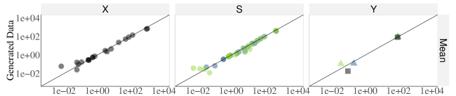
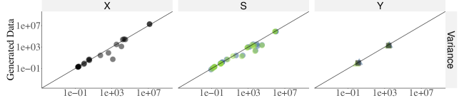
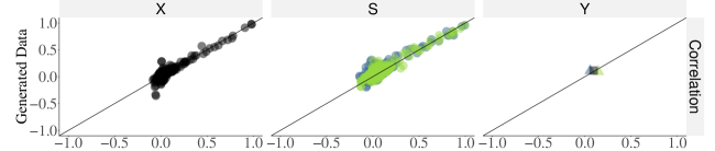
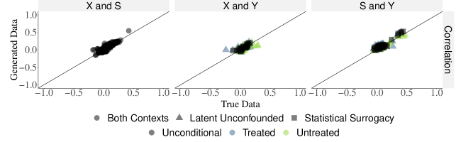
Figure D.4. Validation

Notes: Figure D.4 displays scatterplots comparing the moments of the data from Banerjee et al., (2015) to the GAN generated simulation data. Columns differentiate between different types of variables. In the first three rows, the columns correspond to the pre-treatment covariates, the short-term outcomes, and the long-term outcomes, respectively. The columns of the fourth row correspond to the three pairs of these three variable types. Rows differentiate between different types of moments. The first two rows compare the means and variances of the the true and generated data. The second two rows compare correlations of the true and generated data, within and across variable types, respectively. The x-axis of each sub-panel measures the moments of the true data. The y-axis of each sub-panel measures the moments of the generated data. The x and y axes in the first two rows are displayed in log-scale. A forty-five degree line is displayed in all sub-panels. Triangular and square dots correspond to data generated the Latent Unconfounded Treatment and Statistical Surrogacy Models, respectively. Circular dots correspond to data shared by both models. Blue and green dots denote moments conditioned on treatment being set to one and zero, respectively. Black dots denote unconditioned moments.

The joint distributions of the true and generated data match remarkably closely. This match holds both for data generated for the contexts in which treatment is and is not observed in the observational sample, and continues to hold if moments are conditioned on the treatment assignment being set to one and zero, respectively.

Figure D.5 displays histograms comparing the true and generated distributions for the long-term outcomes, conditioned on treatment assignment. These distributions again align remarkably closely. In each case, the distributions have similarly shaped supports and right tails.

Figure D.5. Comparison of True and Generated Long-Term Outcome Distributions

Panel A: Total Consumption

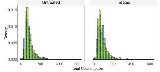
Panel B: Total Assets

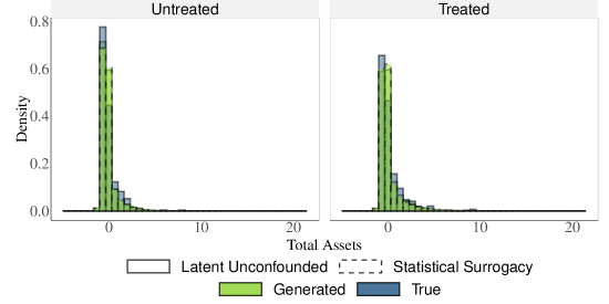
Notes: Figure D.5 displays histograms comparing the true and generated long term outcome distributions, conditioned by treatment assignment. Panel A compares the distributions for total consumption. Panel B compares distributions for total assets. Histograms for the generated and true data are displayed in green and blue, respectively. Solid and dotted lines border the histograms for the data generated for Latent Unconfounded Treatment and Statistical Surrogacy Models, respectively.

D.3. Design

To generate an observation $A_{i}$, we first generate a value of the pre-treatment covariates $X_{i}$ from the first GAN. This generated value of $X_{i}$ is then input into the second GAN to generate values of the treated and untreated short-term potential outcomes, i.e., generating $S_{i}(1)$ and $S_{i}(0)$ by taking draws from the GAN approximating the distributions of $S_{i}|X_{i},W_{i}=1$ and $S_{i}|X_{i},W_{i}=0$. We repeat this step, using the generated values $(X_{i},S(1))$ and $(X_{i},S_{i}(0))$ as inputs into the third GAN to generate the long-term treated and untreated potential outcomes $Y_{i}(1)$ and $Y_{i}(0)$, respectively. Each observation is assigned to being either “experimental” or “observational” uniformly at random, i.e., we draw each $G_{i}$ from a Bernoulli distribution with parameter $1/2$. Treatment is always assigned uniformly at random for experimental observations.

We consider two procedures for assigning treatment for the observational units. First, as a baseline, we assign treatment uniformly at random, leaving treatment assignment unconfounded. Second, we induce confounding. Specifically, we assign treatment with probability

$$\frac{1}{1+\exp(-(\tilde{\tau}_{c,i}+\tilde{\tau}_{a,i})\cdot\phi)}$$

where $\tilde{\tau}_{c,i}$ and $\tilde{\tau}_{a,i}$ denote the true treatment effects on short-term total consumption and total assets for unit $i$, normalized across observational units, and $\phi$ is a parameter indexing the degree of confounding. Written differently, the probability of being assigned treatment increases logistically with the true treatment effects on short-term outcomes. Large values of $\phi$ induce more confounding.

By repeating this process, we generate ten million simulation draws. We take the empirical distribution of this sample as the population distribution. In this sample, we observe both treated and untreated potential outcomes, and, thereby, the true treatment effects for each individual. It is worth noting the significant computational scale of the experiment reported in this section. The simulation requires parallelization on a large-scale computing cluster and uses roughly 60 years of cpu time.

Panel A of Figure D.6 plots the probability that an observational unit is assigned to treatment as a function of $\tilde{\tau}_{c,i}$ and $\tilde{\tau}_{a,i}$, the true treatment effects on short-term total consumption and total assets for unit $i$, normalized across observational units. This curve is displayed for $\phi$ equal to $0.50$ and $0.66$, which are the parameter values that we consider in out simulation analysis. Panels B and C display histograms of the treatment probabilities for all of the simulation draws for $\phi$ equal to $0.50$ and $0.66$. Observe that increasing $\phi$ increases the confounding in the data, in the sense that there are more simulation draws with propensity scores very different from one half.

Figure D.6. Visualization of Confounding Parameterization

Panel A: Parameterization of Confounding
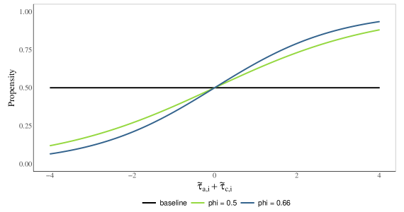
Panel B: Histogram of Propensities, $\phi=0.5$	Panel C: Histogram of Propensities, $\phi=0.66$

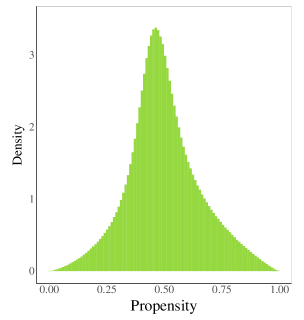
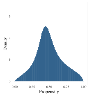
Notes: Panel A of Figure D.6 displays curves giving the probability of a simulation draw being assigned to treatment as a function of $\tilde{\tau}_{c,i}$ and $\tilde{\tau}_{a,i}$, the true treatment effects on short-term total consumption and total assets for unit $i$, normalized across observational units. Panels B and C display histograms of the treatment probabilities for all simulation draws for $\phi$ equal to $0.50$ and $0.66$, respectively.

D.4. Estimation Details

Cross-fitting:

Following the choice made in Chernozhukov et al., (2018), we set $k$ equal to five for the $k$-fold cross-fitting construction. We expect that alternative choices for this hyper-parameter will not impact the results of the simulation substantially, and so do not report results for different choices of $k$.

Propensity Score Estimation:

For the sake of numerical stability across simulations, we threshold all estimates of propensity scores to lie in $[0.05,0.95]$, which amounts to enforcing a value of $\varepsilon$ chosen for the strict overlap Assumption 2.2 in the estimation of propensity scores. The choice of this hyper-parameter may substantively impact results in cases, e.g., in which the covariate distributions of the experimental and observational distributions have limited overlap. We do not report results for alternative choices of these hyperparameters, but view the adaptation of the methods developed in Section 4 to setting in which there is limited overlap along one or more direction as a useful direction for further research.

Linear Regression:

We use ordinary linear regression and a generalized linear model with a binomial response type when estimating outcome mean and propensity score type nuisance functions, respectively.

Lasso:

We implement cross-validated Lasso (Tibshirani,, 1996) with the R package “glmnet’ (Hastie and Qian,, 2014). In each cross-fitting fold, we use $5$-fold cross-validation to choose the regularization parameter that gives the minimum mean cross-validation error. We use the binomial response type when estimating propensity scores.

GRF:

We implement generalized random forests (Athey et al.,, 2019) with the R package “grf”. When $h\in\{1,3\}$, we set the “honesty” hyper-parameter equal to false. In each cross-fitting fold, we choose the hyper-parameters “sample.fraction”, “mtry”, and “min.node.size” by setting the grf hyper-parameter “tune.parameters” equal to “all”. This option chooses $1000$ hyper-parameter values randomly, then chooses the hyper-parameter values with the minimum 5-fold cross-validation error. When $h=10$, we set “sample.fraction” equal to 0.1 in order to optimize memory usage, but tuned the other parameters in the same manner. We use regression forests to predict both long-term outcome means and propensity scores.

XGBoost:

We implement XGboost (Chen and Guestrin,, 2016) with the R package “xgboost” (Chen et al.,, 2015). We set the learning rate $\eta$ and max depth equal to $0.1$ and $2$, respectively. We choose the number of rounds with 5-fold cross validation, with the maximum number of rounds set to $100$. We use the root mean squared error and log-loss as the evaluation metrics for the estimation of long-term outcome means and propensity scores, respectively.

D.5. Additional Results

Figures D.7 and D.8 displays results analogous to Figures 2 and 3 in the main text, when total household consumption is chosen as the long-term outcome of interest. The results are very similar to the those reported in the main text.

Figure D.7. Comparison of Estimators

Panel A: Latent Unconfounded Treatment

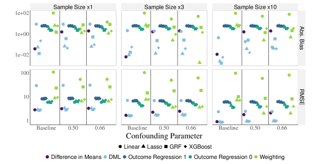
Panel B: Statistical Surrogacy

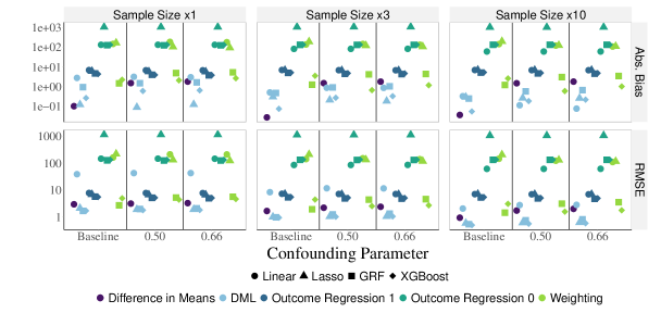
Notes: Figure D.7 compares measurements of the absolute bias and root mean squared error for the estimators formulated in Section 4, in addition to the difference in means estimator defined in (5.1). The y-axes are displayed in logs, base 10. The long-term outcome is total household consumption. Panels A and B display results for the Latent Unconfounded Treatment and Statistical Surrogacy Models defined in 2.1 and 2.2, respectively. The columns of each panel vary the sample size multiplier $h$. Each sub-panel displays results for the baseline, unconfounded, case, as well as for the cases that the confounding parameter $\phi$ has been set to $1/2$ and $2/3$. Results for each estimator are displayed with dots of different colors. Results for different nuisance parameter estimators are displayed with dots of different shapes.

Figure D.8. Finite-Sample Performance with Different Nuisance Parameter Estimators

Panel A: Latent Unconfounded Treatment

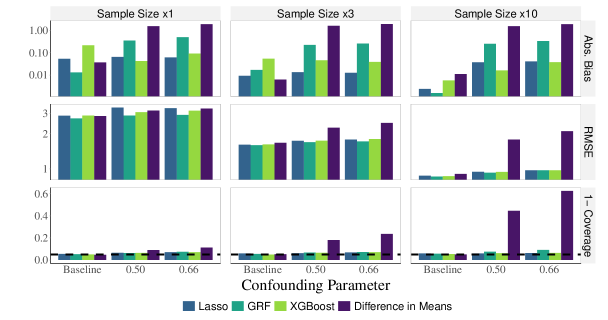
Panel B: Statistical Surrogacy

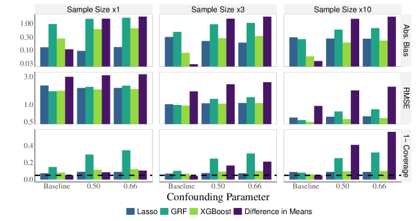
Notes: Figure D.8 displays measurements of the quality of the estimators formulated in Section 4.1 implemented with several alternative choices of nuisance parameter estimators. The long-term outcome is total household consumption. Panels A and B display results for the estimators defined in 4.1 for the Latent Unconfounded Treatment and Statistical Surrogacy Models defined in 2.1 and 2.2, respectively. The columns of each panel vary the sample size multiplier $h$. The rows of each panel display the absolute value of the bias, one minus the coverage probability, and the root mean squared error of each estimator, from top to bottom, respectively. A dotted line denoting one minus the nominal coverage probability, 0.05, is displayed in each sub-panel in the third row. Each sub-panel displays a bar graph comparing measurements of the performance of the estimator defined in 4.1, constructed with three types of nuisance parameter estimators, with the difference in means estimator (5.1). Each sub-panel displays results for the baseline, unconfounded, case, as well as for the cases that the confounding parameter $\phi$ has been set to $1/2$ and $2/3$.

Figure D.9. Comparison of Estimators

Panel A: Latent Unconfounded Treatment

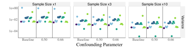
Panel B: Statistical Surrogacy

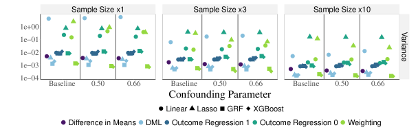
Notes: Figure D.9 compares measurements of variance for the estimators formulated in Section 4, in addition to the difference in means estimator defined in (5.1). The y-axes are displayed in logs, base 10. The long-term outcome is total household assets. All other formatting is analogous to Figure 2 in the main text.

Figure D.10. Comparison of Estimators

Panel A: Latent Unconfounded Treatment

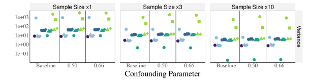
Panel B: Statistical Surrogacy

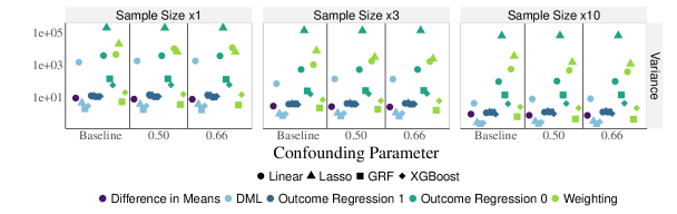
Notes: Figure D.10 compares measurements of variance for the estimators formulated in Section 4, in addition to the difference in means estimator defined in (5.1). The y-axes are displayed in logs, base 10. The long-term outcome is total household consumption. All other formatting is analogous to Figure D.7

Tables 2 and 3 present estimates of coverage probabilities of confidence intervals constructed around the estimators formulated in 4.1. Wald intervals constructed around the difference in means estimator severely undercover when there is confounding in the observational data set. The confidence intervals (A.41) tend to undercover, although the under-coverage is not as severe. Coverage is worse under the Statistical Surrogacy Model and is very poor when generalized random forests are used to estimate nuisance parameters. This is a result of the bias exhibited in Figure 3 and Figure D.8. By contrast, in the same situation, the coverage probabilities are much closer to the nominal level when nuisance parameters are estimated with the Lasso or XGBoost. As an exception, these intervals over cover if nuisance parameters are estimated with linear regression.

		Treatment Observed				Treatment Not Observed
	Confounding:	Baseline	0.5	0.66		Baseline	0.5	0.66
	Sample Size:	(1)	(2)	(3)		(4)	(5)	(6)
Difference in Means	$\times 1$	0.953	0.803	0.712		0.953	0.811	0.735
	$\times 3$	0.956	0.545	0.353		0.955	0.564	0.396
	$\times 10$	0.953	0.095	0.011		0.954	0.101	0.021
Linear	$\times 1$	0.992	0.995	0.994		0.976	0.979	0.977
	$\times 3$	0.999	0.999	1.000		0.974	0.981	0.983
	$\times 10$	1.000	1.000	1.000		0.946	0.983	0.985
Lasso	$\times 1$	0.946	0.908	0.901		0.904	0.862	0.843
	$\times 3$	0.945	0.922	0.911		0.823	0.877	0.884
	$\times 10$	0.945	0.930	0.929		0.522	0.742	0.784
GRF	$\times 1$	0.947	0.901	0.868		0.791	0.438	0.334
	$\times 3$	0.947	0.900	0.877		0.882	0.520	0.405
	$\times 10$	0.946	0.842	0.743		0.905	0.583	0.467
XGBoost	$\times 1$	0.947	0.908	0.891		0.868	0.784	0.746
	$\times 3$	0.952	0.909	0.900		0.916	0.834	0.807
	$\times 10$	0.949	0.925	0.916		0.917	0.849	0.839

Table 2. Coverage Probability Estimates: Total Assets

Notes: Table 2 compares estimates of the coverage probabilities of confidence intervals constructed around each estimator. The long-term outcome of interest is taken to be total assets. The nominal coverage probability is set to $0.95$ in each case. Standard Wald intervals are constructed around the difference in means estimator (5.1). Confidence intervals are constructed with (A.41) for the estimators formulated in 4.1.

		Treatment Observed				Treatment Not Observed
	Confounding:	Baseline	0.5	0.66		Baseline	0.5	0.66
	Sample Size:	(1)	(2)	(3)		(4)	(5)	(6)
Difference in Means	$\times 1$	0.953	0.910	0.887		0.948	0.914	0.895
	$\times 3$	0.948	0.820	0.763		0.957	0.834	0.788
	$\times 10$	0.950	0.554	0.374		0.949	0.590	0.436
Linear	$\times 1$	0.994	0.997	0.996		0.985	0.983	0.985
	$\times 3$	0.999	1.000	0.999		0.985	0.984	0.985
	$\times 10$	1.000	1.000	1.000		0.987	0.986	0.983
Lasso	$\times 1$	0.945	0.935	0.929		0.926	0.909	0.910
	$\times 3$	0.941	0.938	0.931		0.930	0.924	0.926
	$\times 10$	0.941	0.940	0.937		0.910	0.910	0.909
GRF	$\times 1$	0.948	0.937	0.926		0.852	0.705	0.654
	$\times 3$	0.945	0.932	0.928		0.898	0.753	0.692
	$\times 10$	0.943	0.925	0.908		0.918	0.747	0.680
XGBoost	$\times 1$	0.950	0.936	0.929		0.918	0.884	0.877
	$\times 3$	0.951	0.934	0.929		0.931	0.905	0.899
	$\times 10$	0.946	0.938	0.935		0.937	0.903	0.898

Table 3. Coverage Probability Estimates: Total Consumption

Notes: Table 3 compares estimates of the coverage probabilities of confidence intervals constructed around each estimator. The long-term outcome of interest is taken to be total consumption. The nominal coverage probability is set to $0.95$ in each case. Standard Wald intervals are constructed around the difference in means estimator (5.1). Confidence intervals are constructed with (A.41) for the estimators formulated in 4.1.

References

- \NAT@swatrue
- (1) Athey, S., Chetty, R., and Imbens, G. (2020a). Combining experimental and observational data to estimate treatment effects on long term outcomes. arXiv preprint arXiv:2006.09676. \NAT@swatrue
- (2) Athey, S., Chetty, R., Imbens, G., and Kang, H. (2020b). Estimating treatment effects using multiple surrogates: The role of the surrogate score and the surrogate index. \NAT@swatrue
- Athey and Imbens, (2017) Athey, S. and Imbens, G. W. (2017). The state of applied econometrics: Causality and policy evaluation. Journal of Economic Perspectives, 31(2):3–32. \NAT@swatrue
- Athey et al., (2021) Athey, S., Imbens, G. W., Metzger, J., and Munro, E. (2021). Using wasserstein generative adversarial networks for the design of monte carlo simulations. Journal of Econometrics. \NAT@swatrue
- Athey et al., (2018) Athey, S., Imbens, G. W., and Wager, S. (2018). Approximate residual balancing: debiased inference of average treatment effects in high dimensions. Journal of the Royal Statistical Society: Series B (Statistical Methodology), 80(4):597–623. \NAT@swatrue
- Athey et al., (2019) Athey, S., Tibshirani, J., and Wager, S. (2019). Generalized random forests. The Annals of Statistics, 47(2):1148–1178. \NAT@swatrue
- Banerjee et al., (2015) Banerjee, A., Duflo, E., Goldberg, N., Karlan, D., Osei, R., Parienté, W., Shapiro, J., Thuysbaert, B., and Udry, C. (2015). A multifaceted program causes lasting progress for the very poor: Evidence from six countries. Science, 348(6236). \NAT@swatrue
- Bang and Robins, (2005) Bang, H. and Robins, J. M. (2005). Doubly robust estimation in missing data and causal inference models. Biometrics, 61(4):962–973. \NAT@swatrue
- Begg and Leung, (2000) Begg, C. B. and Leung, D. H. (2000). On the use of surrogate end points in randomized trials. Journal of the Royal Statistical Society: Series A (Statistics in Society), 163(1):15–28. \NAT@swatrue
- Belloni et al., (2014) Belloni, A., Chernozhukov, V., and Wang, L. (2014). Pivotal estimation via square-root Lasso in nonparametric regression. The Annals of Statistics, 42(2):757 – 788. \NAT@swatrue
- Bia et al., (2020) Bia, M., Huber, M., and Lafférs, L. (2020). Double machine learning for sample selection models. arXiv preprint arXiv:2012.00745. \NAT@swatrue
- Bickel, (1982) Bickel, P. J. (1982). On adaptive estimation. The Annals of Statistics, pages 647–671. \NAT@swatrue
- Bickel et al., (1993) Bickel, P. J., Klaassen, C. A., Ritov, Y., and Wellner, J. A. (1993). Efficient and adaptive estimation for semiparametric models, volume 4. Johns Hopkins University Press Baltimore. \NAT@swatrue
- Bickel et al., (2009) Bickel, P. J., Ritov, Y., and Tsybakov, A. B. (2009). Simultaneous analysis of lasso and dantzig selector. The Annals of statistics, 37(4):1705–1732. \NAT@swatrue
- Bouguen et al., (2019) Bouguen, A., Huang, Y., Kremer, M., and Miguel, E. (2019). Using randomized controlled trials to estimate long-run impacts in development economics. Annual Review of Economics. \NAT@swatrue
- Bradic et al., (2019) Bradic, J., Wager, S., and Zhu, Y. (2019). Sparsity double robust inference of average treatment e ects. \NAT@swatrue
- Chen and Guestrin, (2016) Chen, T. and Guestrin, C. (2016). Xgboost: A scalable tree boosting system. In Proceedings of the 22nd acm sigkdd international conference on knowledge discovery and data mining, pages 785–794. \NAT@swatrue
- Chen et al., (2015) Chen, T., He, T., Benesty, M., Khotilovich, V., Tang, Y., Cho, H., et al. (2015). Xgboost: extreme gradient boosting. R package version 0.4-2, 1(4):1–4. \NAT@swatrue
- Chen, (2007) Chen, X. (2007). Large sample sieve estimation of semi-nonparametric models. Handbook of econometrics, 6:5549–5632. \NAT@swatrue
- Chen et al., (2008) Chen, X., Hong, H., and Tarozzi, A. (2008). Semiparametric efficiency in GMM models with auxiliary data. The Annals of Statistics, 36(2):808 – 843. \NAT@swatrue
- Chen and Liao, (2015) Chen, X. and Liao, Z. (2015). Sieve semiparametric two-step gmm under weak dependence. Journal of Econometrics, 189(1):163–186. \NAT@swatrue
- Chen et al., (2014) Chen, X., Liao, Z., and Sun, Y. (2014). Sieve inference on possibly misspecified semi-nonparametric time series models. Journal of Econometrics, 178:639–658. \NAT@swatrue
- Chen and Santos, (2018) Chen, X. and Santos, A. (2018). Overidentification in regular models. Econometrica, 86(5):1771–1817. \NAT@swatrue
- Chen and Shen, (1998) Chen, X. and Shen, X. (1998). Sieve extremum estimates for weakly dependent data. Econometrica, pages 289–314. \NAT@swatrue
- Chen and White, (1999) Chen, X. and White, H. (1999). Improved rates and asymptotic normality for nonparametric neural network estimators. IEEE Transactions on Information Theory, 45(2):682–691. \NAT@swatrue
- Chernozhukov et al., (2018) Chernozhukov, V., Chetverikov, D., Demirer, M., Duflo, E., Hansen, C., Newey, W., and Robins, J. (2018). Double/debiased machine learning for treatment and structural parameters. The Econometrics Journal, 21:C1–C68. \NAT@swatrue
- Chernozhukov et al., (2016) Chernozhukov, V., Escanciano, J. C., Ichimura, H., Newey, W. K., and Robins, J. M. (2016). Locally robust semiparametric estimation. arXiv preprint arXiv:1608.00033. \NAT@swatrue
- Crump et al., (2009) Crump, R. K., Hotz, V. J., Imbens, G. W., and Mitnik, O. A. (2009). Dealing with limited overlap in estimation of average treatment effects. Biometrika, 96(1):187–199. \NAT@swatrue
- Dal Bó et al., (2021) Dal Bó, E., Finan, F., Li, N. Y., and Schechter, L. (2021). Information technology and government decentralization: Experimental evidence from paraguay. Econometrica, 89(2):677–701. \NAT@swatrue
- Duflo et al., (2007) Duflo, E., Glennerster, R., and Kremer, M. (2007). Using randomization in development economics research: A toolkit. Handbook of development economics, 4:3895–3962. \NAT@swatrue
- Dynarski et al., (2021) Dynarski, S., Libassi, C., Michelmore, K., and Owen, S. (2021). Closing the gap: The effect of reducing complexity and uncertainty in college pricing on the choices of low-income students. American Economic Review, 111(6):1721–56. \NAT@swatrue
- D’Amour et al., (2021) D’Amour, A., Ding, P., Feller, A., Lei, L., and Sekhon, J. (2021). Overlap in observational studies with high-dimensional covariates. Journal of Econometrics, 221(2):644–654. \NAT@swatrue
- Farrell et al., (2021) Farrell, M. H., Liang, T., and Misra, S. (2021). Deep neural networks for estimation and inference. Econometrica, 89(1):181–213. \NAT@swatrue
- Fisher, (1925) Fisher, R. A. (1925). Statistical methods for research workers. Statistical methods for research workers., (1st. ed). \NAT@swatrue
- Foster and Syrgkanis, (2019) Foster, D. J. and Syrgkanis, V. (2019). Orthogonal statistical learning. arXiv preprint arXiv:1901.09036. \NAT@swatrue
- Frölich, (2007) Frölich, M. (2007). Nonparametric iv estimation of local average treatment effects with covariates. Journal of Econometrics, 139(1):35–75. \NAT@swatrue
- Gechter and Meager, (2021) Gechter, M. and Meager, R. (2021). Combining experimental and observational studies in meta-analysis: A mutual debiasing approach.”. Technical report, Mimeo. \NAT@swatrue
- Gertler et al., (2014) Gertler, P., Heckman, J., Pinto, R., Zanolini, A., Vermeersch, C., Walker, S., Chang, S. M., and Grantham-McGregor, S. (2014). Labor market returns to an early childhood stimulation intervention in jamaica. Science, 344(6187):998–1001. \NAT@swatrue
- Goodfellow et al., (2014) Goodfellow, I., Pouget-Abadie, J., Mirza, M., Xu, B., Warde-Farley, D., Ozair, S., Courville, A., and Bengio, Y. (2014). Generative adversarial nets. Advances in neural information processing systems, 27. \NAT@swatrue
- Graham, (2011) Graham, B. S. (2011). Efficiency bounds for missing data models with semiparametric restrictions. Econometrica, 79(2):437–452. \NAT@swatrue
- Gui, (2020) Gui, G. (2020). Combining observational and experimental data using first-stage covariates. arXiv preprint arXiv:2010.05117. \NAT@swatrue
- Gupta et al., (2019) Gupta, S., Kohavi, R., Tang, D., Xu, Y., Andersen, R., Bakshy, E., Cardin, N., Chandran, S., Chen, N., Coey, D., Curtis, M., Deng, A., Duan, W., Forbes, P., Frasca, B., Guy, T., Imbens, G. W., Saint Jacques, G., Kantawala, P., Katsev, I., Katzwer, M., Konutgan, M., Kunakova, E., Lee, M., Lee, M., Liu, J., McQueen, J., Najmi, A., Smith, B., Trehan, V., Vermeer, L., Walker, T., Wong, J., and Yashkov, I. (2019). Top challenges from the first practical online controlled experiments summit. ACM SIGKDD Explorations Newsletter, 21(1):20–35. \NAT@swatrue
- Hahn, (1998) Hahn, J. (1998). On the role of the propensity score in efficient semiparametric estimation of average treatment effects. Econometrica, pages 315–331. \NAT@swatrue
- Hastie and Qian, (2014) Hastie, T. and Qian, J. (2014). Glmnet vignette. Retrieved June, 9(2016):1–30. \NAT@swatrue
- Hirano et al., (2003) Hirano, K., Imbens, G. W., and Ridder, G. (2003). Efficient estimation of average treatment effects using the estimated propensity score. Econometrica, 71(4):1161–1189. \NAT@swatrue
- Horvitz and Thompson, (1952) Horvitz, D. G. and Thompson, D. J. (1952). A generalization of sampling without replacement from a finite universe. Journal of the American statistical Association, 47(260):663–685. \NAT@swatrue
- Hotz et al., (2005) Hotz, V. J., Imbens, G. W., and Mortimer, J. H. (2005). Predicting the efficacy of future training programs using past experiences at other locations. Journal of Econometrics, 125(1-2):241–270. \NAT@swatrue
- Hou et al., (2021) Hou, J., Mukherjee, R., and Cai, T. (2021). Efficient and robust semi-supervised estimation of ate with partially annotated treatment and response. \NAT@swatrue
- Ichimura and Newey, (2022) Ichimura, H. and Newey, W. K. (2022). The influence function of semiparametric estimators. Quantitative Economics, 13(1):29–61. \NAT@swatrue
- Imai et al., (2010) Imai, K., Keele, L., and Tingley, D. (2010). A general approach to causal mediation analysis. Psychological methods, 15(4):309. \NAT@swatrue
- Imbens et al., (2022) Imbens, G., Kallus, N., Mao, X., and Wang, Y. (2022). Long-term causal inference under persistent confounding via data combination. \NAT@swatrue
- Imbens, (2004) Imbens, G. W. (2004). Nonparametric estimation of average treatment effects under exogeneity: A review. Review of Economics and statistics, 86(1):4–29. \NAT@swatrue
- Kallus and Mao, (2020) Kallus, N. and Mao, X. (2020). On the role of surrogates in the efficient estimation of treatment effects with limited outcome data. arXiv preprint arXiv:2003.12408. \NAT@swatrue
- Kang and Schafer, (2007) Kang, J. D. and Schafer, J. L. (2007). Demystifying double robustness: A comparison of alternative strategies for estimating a population mean from incomplete data. Statistical science, pages 523–539. \NAT@swatrue
- Kennedy, (2022) Kennedy, E. H. (2022). Semiparametric doubly robust targeted double machine learning: a review. arXiv preprint arXiv:2203.06469. \NAT@swatrue
- Kennedy, (2023) Kennedy, E. H. (2023). Semiparametric doubly robust targeted double machine learning: a review. \NAT@swatrue
- Klaassen, (1987) Klaassen, C. A. J. (1987). Consistent Estimation of the Influence Function of Locally Asymptotically Linear Estimators. The Annals of Statistics, 15(4):1548 – 1562. \NAT@swatrue
- Le Cam, (1956) Le Cam, L. (1956). On the asymptotic theory of estimation and testing hypotheses. In Proceedings of the Third Berkeley Symposium on Mathematical Statistics and Probability, Volume 1: Contributions to the Theory of Statistics, volume 3, pages 129–157. University of California Press. \NAT@swatrue
- Little and Rubin, (2019) Little, R. J. and Rubin, D. B. (2019). Statistical analysis with missing data, volume 793. John Wiley & Sons. \NAT@swatrue
- Luo and Spindler, (2017) Luo, Y. and Spindler, M. (2017). -boosting for economic applications. American Economic Review, 107(5):270–73. \NAT@swatrue
- Muris, (2020) Muris, C. (2020). Efficient gmm estimation with incomplete data. Review of Economics and Statistics, 102(3):518–530. \NAT@swatrue
- Newey, (1994) Newey, W. K. (1994). The asymptotic variance of semiparametric estimators. Econometrica: Journal of the Econometric Society, pages 1349–1382. \NAT@swatrue
- Newey and McFadden, (1994) Newey, W. K. and McFadden, D. (1994). Large sample estimation and hypothesis testing. Handbook of econometrics, 4:2111–2245. \NAT@swatrue
- Newey and Robins, (2018) Newey, W. K. and Robins, J. R. (2018). Cross-fitting and fast remainder rates for semiparametric estimation. \NAT@swatrue
- Pearl, (1995) Pearl, J. (1995). Causal diagrams for empirical research. Biometrika, 82(4):669–688. \NAT@swatrue
- Prentice, (1989) Prentice, R. L. (1989). Surrogate endpoints in clinical trials: definition and operational criteria. Statistics in medicine, 8(4):431–440. \NAT@swatrue
- Ridder and Moffitt, (2007) Ridder, G. and Moffitt, R. (2007). The econometrics of data combination. Handbook of econometrics, 6:5469–5547. \NAT@swatrue
- Robins et al., (1995) Robins, J. M., Rotnitzky, A., and Zhao, L. P. (1995). Analysis of semiparametric regression models for repeated outcomes in the presence of missing data. Journal of the american statistical association, 90(429):106–121. \NAT@swatrue
- Rosenbaum and Rubin, (1983) Rosenbaum, P. R. and Rubin, D. B. (1983). The central role of the propensity score in observational studies for causal effects. Biometrika, 70(1):41–55. \NAT@swatrue
- Rosenman et al., (2020) Rosenman, E., Basse, G., Owen, A., and Baiocchi, M. (2020). Combining observational and experimental datasets using shrinkage estimators. arXiv preprint arXiv:2002.06708. \NAT@swatrue
- Rosenman et al., (2018) Rosenman, E., Owen, A. B., Baiocchi, M., and Banack, H. (2018). Propensity score methods for merging observational and experimental datasets. arXiv preprint arXiv:1804.07863. \NAT@swatrue
- Scharfstein et al., (1999) Scharfstein, D. O., Rotnitzky, A., and Robins, J. M. (1999). Adjusting for nonignorable drop-out using semiparametric nonresponse models. Journal of the American Statistical Association, 94(448):1096–1120. \NAT@swatrue
- Singh, (2021) Singh, R. (2021). A finite sample theorem for longitudinal causal inference with machine learning: Long term, dynamic, and mediated effects. \NAT@swatrue
- Singh, (2022) Singh, R. (2022). Generalized kernel ridge regression for long term causal inference: Treatment effects, dose responses, and counterfactual distributions. \NAT@swatrue
- Tan, (2020) Tan, Z. (2020). Model-assisted inference for treatment effects using regularized calibrated estimation with high-dimensional data. The Annals of Statistics, 48(2):811–837. \NAT@swatrue
- Tanner et al., (2015) Tanner, J. C., Candland, T., and Odden, W. S. (2015). Later impacts of early childhood interventions: a systematic review. Washington: Independent Evaluation Group, World Bank Group. \NAT@swatrue
- Tibshirani, (1996) Tibshirani, R. (1996). Regression shrinkage and selection via the lasso. Journal of the Royal Statistical Society: Series B (Methodological), 58(1):267–288. \NAT@swatrue
- Twitter Engineering, (2021) Twitter Engineering (2021). “We built a causal estimation framework on the idea of statistical ‘surrogacy’ (Athey et al 2016) - when we can’t wait to observe long-run outcomes, we create a model based on intermediate data.”. Tweet, @TwitterEng, 18 Oct, 12:18 P.M. \NAT@swatrue
- van der Laan and Petersen, (2004) van der Laan, M. J. and Petersen, M. L. (2004). Estimation of direct and indirect causal effects in longitudinal studies. \NAT@swatrue
- Van der Vaart, (1998) Van der Vaart, A. W. (1998). Asymptotic statistics. Cambridge university press. \NAT@swatrue
- van der Vaart and Wellner, (1996) van der Vaart, A. W. and Wellner, J. A. (1996). Weak convergence and empirical processes. Springer. \NAT@swatrue
- Viviano and Bradic, (2021) Viviano, D. and Bradic, J. (2021). Dynamic covariate balancing: estimating treatment effects over time. arXiv preprint arXiv:2103.01280. \NAT@swatrue
- Wager and Walther, (2015) Wager, S. and Walther, G. (2015). Adaptive concentration of regression trees, with application to random forests. arXiv preprint arXiv:1503.06388. \NAT@swatrue
- Yang et al., (2020) Yang, J., Eckles, D., Dhillon, P., and Aral, S. (2020). Targeting for long-term outcomes. arXiv preprint arXiv:2010.15835.