MLMOD: Machine Learning Methods for Data-Driven Modeling in LAMMPS

Summary

MLMOD is a software package for incorporating machine learning approaches and models into simulations of microscale mechanics and molecular dynamics in LAMMPS. Recent machine learning approaches provide promising data-driven approaches for learning representations for system behaviors from experimental data and high fidelity simulations. The package faciliates learning and using data-driven models for (i) dynamics of the system at larger spatial-temporal scales (ii) interactions between system components, (iii) features yielding coarser degrees of freedom, and (iv) features for new quantities of interest characterizing system behaviors. MLMOD provides hooks in LAMMPS for (i) modeling dynamics and time-step integration, (ii) modeling interactions, and (iii) computing quantities of interest characterizing system states. The package allows for use of machine learning methods with general model classes including Neural Networks, Gaussian Process Regression, Kernel Models, and other approaches. Here we discuss our prototype C++/Python package, aims, and example usage. The package is integrated currently with the mesocale and molecular dynamics simulation package LAMMPS and PyTorch. The source code for this initial version 1.0 of MLMOD has been archived to Zenodo (P. J. Atzberger, 2023). For related papers, examples, updates, and additional information see https://github.com/atzberg/mlmod and http://atzberger.org/.

Statement of Need

A practical challenge in using machine learning methods for simulations is the efforts required to incorporate learned system features to augment existing models and simulation methods. Our package MLMOD aims to address this aspect of data-driven modeling by providing a general interface for incorporating ML models using standardized representations and by leveraging existing simulation frameworks such as LAMMPS (Thompson et al., 2022). Our MLMOD package provides hooks which are triggered during key parts of simulation calculations. In this way standard machine learning frameworks can be used to train ML models, such as PyTorch (Paszke et al., 2019) and TensorFlow (Abadi et al., 2015), with the resulting models more amenable to being translated into practical simulations. The models obtained from learning can be accommodated in many forms, including Deep Neural Networks (DNNs) (Goodfellow et al., 2016), Kernel Regression Models (KRM) (Scholkopf & Smola, 2001), Gaussian Process Regression (GPR) (Rasmussen, 2004), and others (Hastie et al., 2001).

Data-Driven Modeling

Recent advances in machine learning, optimization, and available computational resources are presenting new opportunities for data-driven modeling and simulation in the natural sciences and engineering. Empirical successes in deep learning suggest promising non-linear techniques for learning representations for system behaviors and other underlying features (Goodfellow et al., 2016; Hinton & Salakhutdinov, 2006). Many previous deep learning methods have been developed for problems motivated by image analysis and natural language processing. However, scientific computations and associated dynamical systems present a unique set of challenges for developing and employing recent machine learning approaches (P. J. Atzberger, 2018; Brunton et al., 2016; Schmidt & Lipson, 2009).

In scientific and engineering applications there are often important constraints arising from physical principles required to obtain plausible models and there is a need for results to be more interpretable. In large-scale scientific computations, bottom-up modeling efforts aim to start as close as possible to first principles and perform computations to obtain insights into larger-scale emergent behaviors. Examples include the rheological responses of soft materials and complex fluids from microstructure interactions (Paul J. Atzberger, 2013; Bird, 1987; Kimura, 2009; Lubensky, 1997), molecular dynamics modeling of protein structures and functional domains from atomic level interactions (Brooks et al., 1983; Karplus & McCammon, 2002; McCammon & Harvey, 1988; Thompson et al., 2022), and prediction of weather and climate phenomena from detailed physical models, sensor data, and other measurements (Bauer et al., 2015; Richardson, 2007). Obtaining observables and quantities of interest (QoI) from simulations of such high fidelity detailed models can involve significant computational resources (Giessen et al., 2020; Lusk & Mattsson, 2011; Murr, 2016; Pan, 2021; Sanbonmatsu & Tung, 2007; Washington et al., 2009). Data-driven learning methods present opportunities to formulate more simplified models, provide model flexibility to accommodate subtle effects, or make predictions which are less computationally expensive.

Data-driven modeling can take many forms. As a specific motivation for the package and our initial implementations, we discuss a specific case in detail, but our package also can be used more broadly. In particular, we consider detailed molecular dynamics simulations of large spherical colloidal particles within a bath of much smaller solvent particles. A common problem is to infer interaction laws between the colloidal particles given the surrounding environment arising from the type of solution, charge, and other physical conditions. There is extensive theoretical literature on colloidal interactions and approximate models (Derjaguin, 1941; Doi, 2013; Jones et al., 2002). While analytic approaches have had success, there are many settings where challenges remain which limit the accuracy (Jones et al., 2002; Sidhu et al., 2018). Computational modeling and simulation provides opportunities for capturing phenomena in more physical detail and with better understanding of contributing effects.

While simulations of colloids including the solvent and other environmental factors can be used for making predictions, such computations can be expensive given the many degrees of freedom and small time-scales of solvent-solvent interactions. Colloid coarse-grained models are sought which utilize separation in scales, such as the contrast in size with the solvent and dynamical time-scales. In these circumstances, coarse-grained models aim to capture the effective colloidal interactions and their dynamics.

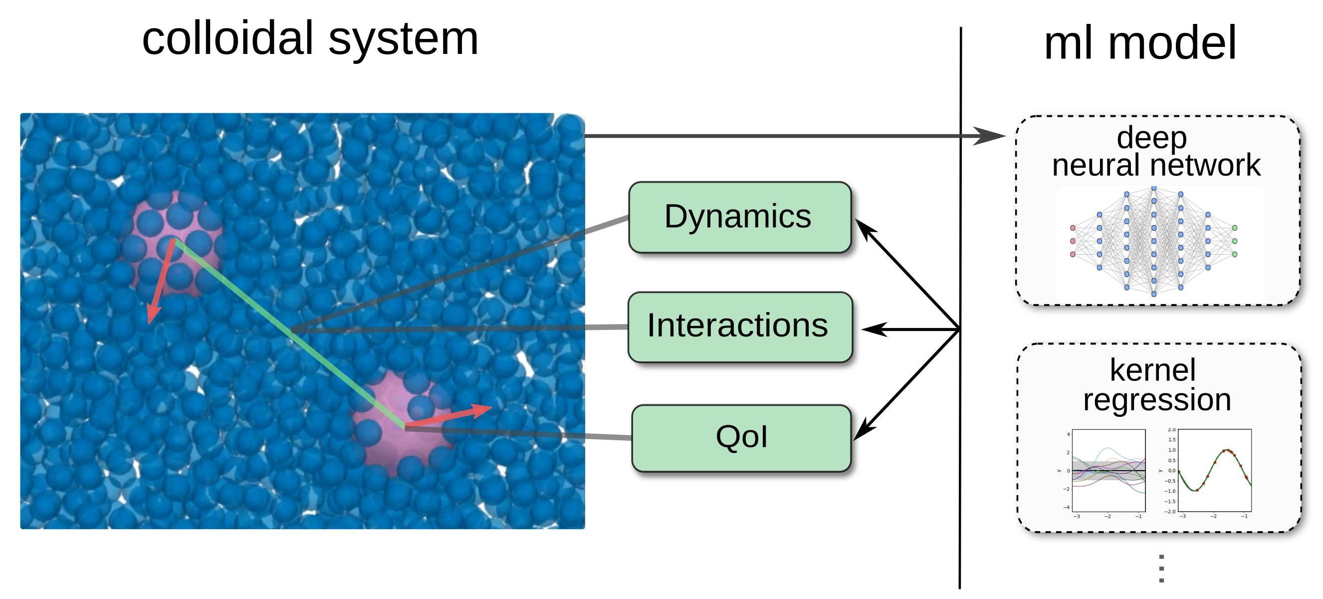
Figure 1: Data-driven modeling from detailed molecular simulations can be used to train machine learning (ML) models for performing simulations at larger spatial-temporal scales. This can include models for the dynamics, interactions, or for computing quantities of interest (QoI) characterizing the system state. The colloidal system for example could be modeled by dynamics at a larger scale with a mobility $M$ obtained from training. In the MLMOD package, the ML models can be represented by Deep Neural Networks, Kernel Regression Models, or other model classes.

Relative to detailed molecular dynamics simulations, this motivates a simplified model for the effective colloid dynamics

$$\frac{d\mathbf{X}}{dt}=\mathbf{M}(\mathbf{X})\mathbf{F}+k_{B}{T}\nabla_{X}\cdot\mathbf{M}(\mathbf{X})+\mathbf{g}$$

$$<\mathbf{g}(s)\mathbf{g}(t)^{T}>=2k_{B}{T}\mathbf{M}(\mathbf{X})\delta(t-s).$$

The $\mathbf{X}\in\mathbb{R}^{3n}$ refers to the collective configuration of all $n$ colloids in these Smoluchowski dynamics (Smoluchowski, 1906). The $\mathbf{g}(t)$ gives the thermal fluctuations for the temperature corresponding to $k_{B}{T}$. Here, the main objectives in this model are to determine (i) the mobility tensor $M=M(\mathbf{X})$ which captures the effective dynamic coupling between the colloidal particles, and (ii) the interaction laws $\mathbf{F}$ for configurations $\mathbf{X}$.

Machine learning methods provide data-driven approaches for learning representations and features for such modeling. Optimization using appropriate loss functions and training protocols can be used to identify system features underlying interactions, symmetries, and other structures. In machine learning methods this is accomplished by using a class of representations and by training with data to identify models from this class. For making predictions in unobserved cases, this allows for interpolation, and in some cases even extrapolation, especially when using explicit low dimensional latent spaces or when imposing other inductive biases (Lopez & Atzberger, 2022; Stinis et al., 2023). For example, consider the colloidal example in the simplified case when we assume the interactions can be approximated as pairwise. The problem reduces to a model $M=M(\mathbf{X}_{1},\mathbf{X}_{2})$ depending on six dimensions. This can be further constrained to learn only symmetric positive semi-definite tensors, for example by learning $L=L(\mathbf{X}_{1},\mathbf{X}_{2})$ to generate $M=LL^{T}$.

There are many ways we can obtain the model $M$. For example, a common way to estimate mobility in fluid mechanics is to apply active forces $\mathbf{F}$ and compute the velocity response $<\mathbf{V}>=<{d\mathbf{X}}/{dt}>\approx\tau^{-1}<\Delta_{\tau}\mathbf{X}(t)>\approx\mathbf{M}\mathbf{F}$. The $\Delta_{\tau}\mathbf{X}(t)=\mathbf{X}(t+\tau)-\mathbf{X}(t)$ for $\tau$ chosen carefully. For large enough forces $\mathbf{F}$, the thermal fluctuations can be averaged away readily by repeating this measurement and taking the mean. In statistical mechanics, another estimator is obtained when $\mathbf{F}=0$ by using the passive fluctuations of system. A moment-based estimator commonly used is $M(\mathbf{X})\approx({2k_{B}{T}\tau)^{-1}}<\Delta_{\tau}\mathbf{X}(t)\Delta_{\tau}\mathbf{X}(t)^{T}>$ for $\tau$ chosen carefully. While theoretically each of these estimators give information on $M$, in practice there can be subtleties such as a good choice for $\tau$, magnitude for $\mathbf{F}$, and role of fluctuations. Even for these more traditional estimators, it could still be useful for storage efficiency and convenience to train an ML model to provide a compressed representation and for interpolation for evaluating $M(\mathbf{X})$.

Machine learning methods also could be used to train more directly from simulation data for sampled colloid trajectories $\mathbf{X}(t)$ (Nielsen et al., 2000; Stinis et al., 2023). The training would select an ML model $M_{\theta}$ over some class of models $H$ parameterized by $\theta$, such as the weights and biases of a Deep Neural Network. For instance, this could be done by Maximum Likelihood Estimation (MLE) or other losses from the trajectory data $\mathbf{X}(t)$. The MLE optimizes the objective

$$M_{\theta}=\arg\min_{M_{\theta}\in{H}}-\log\rho_{\theta}(\mathbf{X}(t_{1}),\mathbf{X}(t_{2}),\ldots,\mathbf{X}(t_{m})).$$

The $\rho_{\theta}$ denotes the likelihood probability density for the model with $M=M_{\theta}$ and observing the trajectory data $\{\mathbf{X}(t_{i})\}$. To obtain tractable and robust training algorithms, further approximations and regularizations may be required to the MLE problem or alternatives used. This could include using variational inference approaches, further restrictions on the model architectures, priors, or other information (Blei et al., 2017; Kingma & Welling, 2014; Lopez & Atzberger, 2020; Stinis et al., 2023). Combining such approximations with further regularizations also could help facilitate learning, including of possible symmetries and other features of trained models $M(\mathbf{X})=M_{\theta}$.

The MLMOD package provides ways for transferring such learned models into practical simulations within LAMMPS. We discussed here one example of a basic data-driven modeling approach for colloids. The MLMOD package can be used more generally and supports broad classes of models for incorporating machine learning results into simulation components. Components can include the dynamics, interactions, or computing quantities of interest. The initial implementations we present supports the basic mobility modeling framework as a proof-of-concept, with longer-term aims to support more general classes of reduced dynamics and interactions in future releases.

Structure of the Package Components

The package is organized as a module within LAMMPS that is called each time-step and has the potential to serve multiple roles within simulations. This includes (i) serving as a time-step integrator updating the configuration of the system based on a specified learned model, (ii) evaluating interactions between system components to compute energy and forces, and (iii) computing quantities of interest (QoI) that can be used as state information during simulations or in statistics. The package is controlled by external XML files that specify the mode of operation and source for pre-trained models and other information, see the schematic in Figure 2.

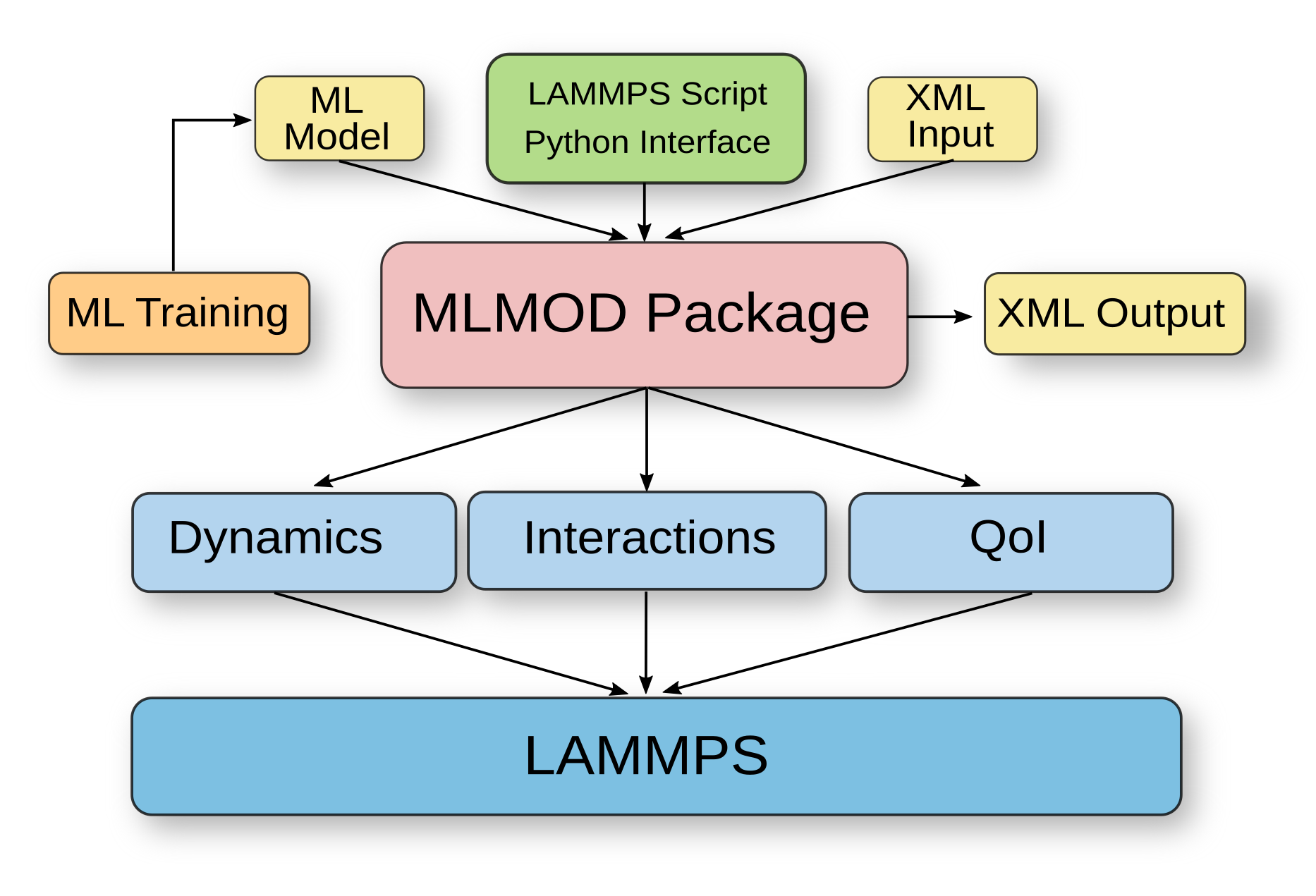
Figure 2: The MLMOD Package is structured modularly with subcomponents for providing ML models in simulations for the dynamics, interactions, and computing quantities of interest (QoI) characterizing the system state. The package makes use of standardized data formats such as XML for inputs and export ML model formats from machine learning frameworks.

The MLMOD Package is incorporated into a simulation by either using the LAMMPS scripting language or the python interface. This is done using the “fix” command in LAMMPS (Thompson et al., 2022), with this terminology historically motivated by algorithms for “fixing” molecular bonds as rigid each time-step. For our package the command to set up the triggers for our algorithms is fix m1 mlmod all filename.mlmod_params. This specifies the tag “m1” for this fix, particle groups controlled by the package as “all”, and the XML file of parameters. The XML file filename.mlmod_params specifies the MLMOD simulation mode and where to find the associated exported ML models. An example and more details are discussed below in the section on package usage. The MLMOD Package can evaluate machine learning models using frameworks such as C++ PyTorch API. This allows both for the possibility of doing on-the-fly learning and for using trained models to augment simulations.

A common approach would be to learn ML models by training on trajectory data from detailed high fidelity simulations using a machine learning framework, such as PyTorch (Paszke et al., 2019). Once the model is trained, it can be exported to a portable format such as Torch (Collobert et al., 2011). The MLMOD package would import these pre-trained models from Torch files such as trained_model.pt. This allows for these models to then be invoked by MLMOD to provide elements for (i) performing time-step integration to model dynamics, (ii) computing interactions between system components, and (iii) computing quantities of interest (QoI) for further computations or as statistics. This provides a modular and general way for data-driven models obtained from training with machine learning methods to be used to govern LAMMPS simulations.

Example Usage of the Package

We give one basic example usage of the package in the case for modeling colloids using a mobility tensor $M$. To set up the triggers for the MLMOD package during LAMMPS simulations a typical command would look like

fix m1 c_group mlmod model.mlmod_params

The m1 gives the tag for the fix, c_group specifies the label for the group of particles controlled by this instance of the MLMOD package. The mlmod specifies to use the MLMOD package with XML parameter file model.mlmod_params. The XML parameter file controls the package modes and the use of associated exported ML models.

Multiple instances of MLMOD package are permitted and can be used to control different groups of particles by adjusting the c_group. The package is designed with modularity so a mode is first defined in a parameter file and then different sets of algorithms and parameters can be used within the same simulation. For the mobility example, an implementation is given by the MLMOD simulation mode dX_MF_ML1. For this modeling mode, a typical parameter file would look like the following.

<?xml version="1.0" encoding="UTF-8"?>
<MLMOD>
  <model_data type="dX_MF_ML1">
    <M_ii_filename value="M_ii_torch.pt"/>
    <M_ij_filename value="M_ij_torch.pt"/>
  </model_data>
</MLMOD>

This specifies for an assumed mobility tensor of pairwise interactions the models for the self-mobility responses $M_{ii}(\mathbf{X})$ and the pairwise mobility response $M_{ij}(\mathbf{X})=M_{ji}(\mathbf{X})$, where $\mathbf{X}=(\mathbf{X}_{1},\mathbf{X}_{2})$. For example, a hydrodynamic model for interactions when the two colloids of radius $a$ are not too close together is to use the Oseen Tensors $M_{ii}=(6\pi\eta a)^{-1}{I}$ and $M_{ij}=(8\pi\eta r)^{-1}\left({I}+r^{-2}\mathbf{r}\mathbf{r}^{T}\right)$. The $\eta$ is the fluid viscosity, $\mathbf{r}=\mathbf{X}_{i}(t)-\mathbf{X}_{j}(t)$ with $r=\|\mathbf{r}\|$ give the particle separation. The responses are $\mathbf{V}_{\ell}=M_{\ell m}\mathbf{F}_{m}$ with $\ell,m\in\{1,2\}$ and summation notation. For different environments surrounding the colloids, these interactions would be learned from simulation data.

The dX_MF_ML1 mode indicates this type of mobility model has interactions from learned ML models. The ML models are given by the files M_ii_torch.pt and M_ij_torch.pt. Related modes can also be implemented to extend models to capture more complicated interactions or near-field effects. For example, to allow for localized many-body interactions with ML models giving contributions to mobility $M(\mathbf{X})$. In this way MLMOD can be used for hybrid modeling combining ML models with more traditional modeling approaches within a unified framework.

This gives one example, the ML interactions and integrators can be more general using any exported model from the machine learning framework. Currently, the implementation uses PyTorch and the export format based on torch script with .pt files. This allows for a variety of models to be used ranging from those based on Deep Neural Networks, Kernel Regression Models, and others.

Conclusion

The package MLMOD provides capabilities in LAMMPS for incorporating into simulations data-driven models for dynamics and interactions obtained from training with machine learning methods. We describe here our initial implementation. For updates, examples, and additional information please see https://github.com/atzberg/mlmod and http://atzberger.org/.

References

reAbadi, M., Agarwal, A., Barham, P., Brevdo, E., Chen, Z., Citro, C., Corrado, G. S., Davis, A., Dean, J., Devin, M., Ghemawat, S., Goodfellow, I., Harp, A., Irving, G., Isard, M., Jia, Y., Jozefowicz, R., Kaiser, L., Kudlur, M., … Zheng, X. (2015). TensorFlow: Large-scale machine learning on heterogeneous systems. https://www.tensorflow.org/

preAtzberger, Paul J. (2013). Incorporating shear into stochastic eulerian-lagrangian methods for rheological studies of complex fluids and soft materials. Physica D: Nonlinear Phenomena, 265, 57–70. https://doi.org/10.1016/j.physd.2013.09.002

preAtzberger, P. J. (2018). Importance of the mathematical foundations of machine learning methods for scientific and engineering applications. SciML2018 Workshop, Position Paper. https://arxiv.org/abs/1808.02213

preAtzberger, P. J. (2023). MLMOD package v1.0.1. Zenodo. https://doi.org/10.5281/zenodo.8327516

preBauer, P., Thorpe, A., & Brunet, G. (2015). The quiet revolution of numerical weather prediction. Nature, 525(7567), 47–55. https://doi.org/10.1038/nature14956

preBird, C., R.B. (1987). Dynamics of polymeric liquids : Volume II kinetic theory. Wiley-Interscience. https://www.wiley.com/en-us/Dynamics+of+Polymeric+Liquids,+Volume+2:+Kinetic+Theory,+2nd+Edition-p-9780471802440

preBlei, D. M., Kucukelbir, A., & McAuliffe, J. D. (2017). Variational inference: A review for statisticians. Journal of the American Statistical Association, 112(518), 859–877. https://doi.org/10.1080/01621459.2017.1285773

preBrooks, B. R., Bruccoleri, R. E., Olafson, B. D., States, D. J., Swaminathan, S. a, & Karplus, M. (1983). CHARMM: A program for macromolecular energy, minimization, and dynamics calculations. Journal of Computational Chemistry, 4(2), 187–217. https://doi.org/10.1002/jcc.540040211

preBrunton, S. L., Proctor, J. L., & Kutz, J. N. (2016). Discovering governing equations from data by sparse identification of nonlinear dynamical systems. Proceedings of the National Academy of Sciences, 113(15), 3932–3937. https://doi.org/10.1073/pnas.1517384113

preCollobert, R., Kavukcuoglu, K., & Farabet, C. (2011). Torch7: A matlab-like environment for machine learning. BigLearn, NIPS Workshop. https://infoscience.epfl.ch/record/192376?ln=en

preDerjaguin, L., B.; Landau. (1941). Theory of the stability of strongly charged lyophobic sols and of the adhesion of strongly charged particles in solutions of electrolytes. Acta Physico Chemica URSS, 633(14). https://doi.org/10.1016/0079-6816(93)90013-l

preDoi, M. (2013). Soft matter physics. Oxford University Press. https://doi.org/10.1093/acprof:oso/9780199652952.001.0001

preGiessen, E. van der, Schultz, P. A., Bertin, N., Bulatov, V. V., Cai, W., Csányi, G., Foiles, S. M., Geers, M. G. D., González, C., Hütter, M., Kim, W. K., Kochmann, D. M., LLorca, J., Mattsson, A. E., Rottler, J., Shluger, A., Sills, R. B., Steinbach, I., Strachan, A., & Tadmor, E. B. (2020). Roadmap on multiscale materials modeling. Modelling and Simulation in Materials Science and Engineering, 28(4), 043001. https://doi.org/10.1088/1361-651x/ab7150

preGoodfellow, I., Bengio, Y., & Courville, A. (2016). Deep learning. The MIT Press. ISBN: 0262035618

preHastie, T., Tibshirani, R., & Friedman, J. (2001). Elements of statistical learning. Springer New York Inc. https://doi.org/10.1007/978-0-387-84858-7

preHinton, G., & Salakhutdinov, R. (2006). Reducing the dimensionality of data with neural networks. Science, 313(5786), 504–507. https://doi.org/10.1126/science.1127647

preJones, R. A. L., Jones, R. A. L., & R Jones, P. (2002). Soft condensed matter. OUP Oxford. ISBN: 9780198505891

preKarplus, M., & McCammon, J. A. (2002). Molecular dynamics simulations of biomolecules. Nature Structural Biology, 9(9), 646–652. https://doi.org/10.1038/nsb0902-646

preKimura, Y. (2009). Microrheology of soft matter. J. Phys. Soc. Jpn., 78(4), 8–8. https://doi.org/10.1143/JPSJ.78.041005

preKingma, D. P., & Welling, M. (2014). Auto-encoding variational bayes. 2nd International Conference on Learning Representations, ICLR 2014, Banff, AB, Canada, April 14-16, 2014, Conference Track Proceedings. http://arxiv.org/abs/1312.6114

preLopez, R., & Atzberger, P. J. (2020). Variational autoencoders for learning nonlinear dynamics of physical systems. https://arxiv.org/abs/2012.03448

preLopez, R., & Atzberger, P. J. (2022). GD-VAEs: Geometric dynamic variational autoencoders for learning nonlinear dynamics and dimension reductions. arXiv Preprint arXiv:2206.05183. https://arxiv.org/abs/2206.05183

preLubensky, T. C. (1997). Soft condensed matter physics. Solid State Communications, 102(2-3), 187-197-. https://doi.org/10.1016/S0038-1098(96)00718-1

preLusk, M. T., & Mattsson, A. E. (2011). High-performance computing for materials design to advance energy science. MRS Bulletin, 36(3), 169–174. https://doi.org/10.1557/mrs.2011.30

preMcCammon, J. A., & Harvey, S. C. (1988). Dynamics of proteins and nucleic acids. Cambridge University Press. https://doi.org/10.1017/CBO9781139167864

preMurr, L. E. (2016). Computer simulations in materials science and engineering. In Handbook of materials structures, properties, processing and performance (pp. 1–15). Springer International Publishing. https://doi.org/10.1007/978-3-319-01905-5_60-2

preNielsen, J. N., Madsen, H., & Young, P. C. (2000). Parameter estimation in stochastic differential equations: An overview. Annual Reviews in Control, 24, 83–94. https://doi.org/10.1016/S1367-5788(00)90017-8

prePan, J. (2021). Scaling up system size in materials simulation. Nature Computational Science, 1(2), 95–95. https://doi.org/10.1038/s43588-021-00034-x

prePaszke, A., Gross, S., Massa, F., Lerer, A., Bradbury, J., Chanan, G., Killeen, T., Lin, Z., Gimelshein, N., Antiga, L., Desmaison, A., Kopf, A., Yang, E., DeVito, Z., Raison, M., Tejani, A., Chilamkurthy, S., Steiner, B., Fang, L., … Chintala, S. (2019). PyTorch: An imperative style, high-performance deep learning library. In H. Wallach, H. Larochelle, A. Beygelzimer, F. dAlché-Buc, E. Fox, & R. Garnett (Eds.), Advances in neural information processing systems 32 (pp. 8024–8035). Curran Associates, Inc. http://papers.neurips.cc/paper/9015-pytorch-an-imperative- style-high-performance-deep-learning-library.pdf

preRasmussen, C. E. (2004). Gaussian processes in machine learning. In O. Bousquet, U. von Luxburg, & G. Rätsch (Eds.), Advanced lectures on machine learning: ML summer schools 2003, canberra, australia, february 2 - 14, 2003, tübingen, germany, august 4 - 16, 2003, revised lectures (pp. 63–71). Springer Berlin Heidelberg. https://doi.org/10.1007/978-3-540-28650-9_4

preRichardson, L. F. (2007). Weather prediction by numerical process. Cambridge university press. https://archive.org/details/weatherpredictio00richrich

preSanbonmatsu, K., & Tung, C.-S. (2007). High performance computing in biology: Multimillion atom simulations of nanoscale systems. Journal of Structural Biology, 157(3), 470–480. https://doi.org/10.1016/j.jsb.2006.10.023

preSchmidt, M., & Lipson, H. (2009). Distilling free-form natural laws from experimental data. 324, 81–85. https://doi.org/10.1126/science.1165893

preScholkopf, B., & Smola, A. J. (2001). Learning with kernels: Support vector machines, regularization, optimization, and beyond. MIT Press. ISBN: 0262194759

preSidhu, I., Frischknecht, A. L., & Atzberger, P. J. (2018). Electrostatics of nanoparticle-wall interactions within nanochannels: Role of double-layer structure and ion-ion correlations. ACS Omega, 3(9), 11340–11353. https://doi.org/10.1021/acsomega.8b01393

preSmoluchowski, V. (1906). Drei vorträge über diffusion, brownsche molekularbewegung und koagulation von kolloidteilchen. Ann. Phys, 21, 756. https://jbc.bj.uj.edu.pl/Content/387533/PDF/FIZART_SMOLUCHOWSKI_00093.pdf

preStinis, P., Daskalakis, C., & Atzberger, P. J. (2023). SDYN-GANs: Adversarial learning methods for multistep generative models for general order stochastic dynamics. arXiv Preprint arXiv:2302.03663. https://arxiv.org/abs/2302.03663

preThompson, A. P., Aktulga, H. M., Berger, R., Bolintineanu, D. S., Brown, W. M., Crozier, P. S., in ’t Veld, P. J., Kohlmeyer, A., Moore, S. G., Nguyen, T. D., Shan, R., Stevens, M. J., Tranchida, J., Trott, C., & Plimpton, S. J. (2022). LAMMPS - a flexible simulation tool for particle-based materials modeling at the atomic, meso, and continuum scales. Computer Physics Communications, 271, 108171. https://doi.org/10.1016/j.cpc.2021.108171

preWashington, W. M., Buja, L., & Craig, A. (2009). The computational future for climate and earth system models: On the path to petaflop and beyond. Philosophical Transactions of the Royal Society A: Mathematical, Physical and Engineering Sciences, 367(1890), 833–846. https://doi.org/10.1098/rsta.2008.0219

p