Deep Networks Provably Classify Data on Curves

Abstract

Data with low-dimensional nonlinear structure are ubiquitous in engineering and scientific problems. We study a model problem with such structure—a binary classification task that uses a deep fully-connected neural network to classify data drawn from two disjoint smooth curves on the unit sphere. Aside from mild regularity conditions, we place no restrictions on the configuration of the curves. We prove that when (i) the network depth is large relative to certain geometric properties that set the difficulty of the problem and (ii) the network width and number of samples are polynomial in the depth, randomly-initialized gradient descent quickly learns to correctly classify all points on the two curves with high probability. To our knowledge, this is the first generalization guarantee for deep networks with nonlinear data that depends only on intrinsic data properties. Our analysis proceeds by a reduction to dynamics in the neural tangent kernel (NTK) regime, where the network depth plays the role of a fitting resource in solving the classification problem. In particular, via fine-grained control of the decay properties of the NTK, we demonstrate that when the network is sufficiently deep, the NTK can be locally approximated by a translationally invariant operator on the manifolds and stably inverted over smooth functions, which guarantees convergence and generalization.

.tocmtchapter mtchaptersubsection mtappendixnone

1 Introduction

In applied machine learning, engineering, and the sciences, we are frequently confronted with the problem of identifying low-dimensional structure in high-dimensional data. In certain well-structured data sets, identifying a good low-dimensional model is the principal task: examples include convolutional sparse models in microscopy [47] and neuroscience [13, 19], and low-rank models in collaborative filtering [8, 11]. Even more complicated datasets from problems such as image classification exhibit some form of low-dimensionality: recent experiments estimate the effective dimension of CIFAR-10 as 26 and the effective dimension of ImageNet as 43 [65]. The variability in these datasets can be thought of as comprising two parts: a “probabilistic” variability induced by the distribution of geometries associated with a given class, and a “geometric” variability associated with physical nuisances such as pose and illumination. The former is challenging to model analytically; virtually all progress on this issue has come through the introduction of large datasets and high-capacity learning machines. The latter induces a much cleaner analytical structure: transformations of a given image lie near a low-dimensional submanifold of the image space (Figure 1). The celebrated successes of convolutional neural networks in image classification seem to derive from their ability to simultaneously handle both types of variability. Studying how neural networks compute with data lying near a low-dimensional manifold is an essential step towards understanding how neural networks achieve invariance to continuous transformations of the image domain, and towards the longer term goal of developing a more comprehensive mathematical understanding of how neural networks compute with real data. At the same time, in some scientific and engineering problems, classifying manifold-structured data is the goal—one example is in gravitational wave astronomy [25, 34], where the goal is to distinguish true events from noise, and the events are generated by relatively simple physical systems with only a few degrees of freedom.

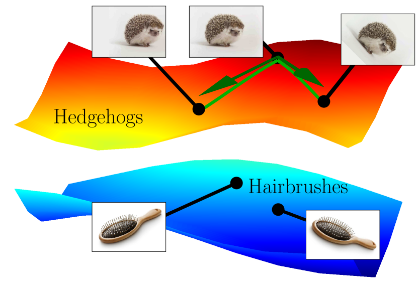
Figure 1: Low-dimensional structure in image data and the two curves problem. Left: Manifold structure in natural images arises due to invariance of the label to continuous domain transformations such as translations and rotations. Right: The two curve problem. We train a neural network to classify points sampled from a density $\rho$ on the submanifolds $\mathcal{M}_{+},\mathcal{M}_{-}$ of the unit sphere. We illustrate the angle injectivity radius $\Delta$ and curvature $1/\kappa$. These parameters help to control the difficulty of the problem: problems with smaller separation and larger curvature are more readily separated with deeper networks.

Motivated by these long term goals, in this paper we study the multiple manifold problem (Figure 1), a mathematical model problem in which we are presented with a finite set of labeled samples lying on disjoint low-dimensional submanifolds of a high-dimensional space, and the goal is to correctly classify every point on each of the submanifolds—a strong form of generalization. The central mathematical question is how the structure of the data (properties of the manifolds such as dimension, curvature, and separation) influences the resources (data samples, and network depth and width) required to guarantee generalization. Our main contribution is the first end-to-end analysis of this problem for a nontrivial class of manifolds: one-dimensional smooth curves that are non-intersecting, cusp-free, and without antipodal pairs of points. Subject to these constraints, the curves can be oriented essentially arbitrarily (say, non-linearly-separably, as in Figure 1), and the hypotheses of our results depend only on architectural resources and intrinsic geometric properties of the data. To our knowledge, this is the first generalization result for training a deep nonlinear network to classify structured data that makes no a-priori assumptions about the representation capacity of the network or about properties of the network after training.

Our analysis proceeds in the neural tangent kernel (NTK) regime of training, where the network is wide enough to guarantee that gradient descent can make large changes in the network output while making relatively small changes to the network weights. This approach is inspired by the recent work [61], which reduces the analysis of generalization in the one-dimensional multiple manifold problem to an auxiliary problem called the certificate problem. Solving the certificate problem amounts to proving that the target label function lies near the stable range of the NTK. The existence of certificates (and more generally, the conditions under which practically-trained neural networks can fit structured data) is open, except for a few very simple geometries which we will review below—in particular, [61] leaves this question completely open. Our technical contribution is to show that setting the network depth sufficiently large relative to intrinsic properties of the data guarantees the existence of a certificate (Theorem 3.1), resolving the one-dimensional case of the multiple manifold problem for a broad class of curves (Theorem 3.2). This leads in turn to a novel perspective on the role of the network depth as a fitting resource in the classification problem, which is inaccessible to shallow networks.

1.1 Related Work

Deep networks and low dimensional structure.

Modern applications of deep neural networks include numerous examples of low-dimensional manifold structure, including pose and illumination variations in image classification [2, 6], as well as detection of structured signals such as electrocardiograms [17, 23], gravitational waves [25, 34], audio signals [16], and solutions to the diffusion equation [52]. Conventionally, to compute with such data one might begin by extracting a low-dimensional representation using nonlinear dimensionality reduction (“manifold learning”) algorithms [58, 4, 60, 5, 3, 7, 15]. For supervised tasks, there is also theoretical work on kernel regression over manifolds [14, 22, 12, 55]. These results rely on very general Sobolev embedding theorems, which are not precise enough to specify the interplay between regularity of the kernel and properties of the data need to obtain concrete resource tradeoffs in the two curve problem. There is also a literature which studies the resource requirements associated with approximating functions over low-dimensional manifolds [33, 48, 42, 18]: a typical result is that for a sufficiently smooth function there exists an approximating network whose complexity is controlled by intrinsic properties such as the dimension. In contrast, we seek algorithmic guarantees that prove that we can efficiently train deep neural networks for tasks with low-dimensional structure. This requires us to grapple with how the geometry of the data influences the dynamics of optimization methods.

Neural networks and structured data—theory?

Spurred by insights in asymptotic infinite width [26, 28] and non-asymptotic [21, 24] settings, there has been a surge of recent theoretical work aimed at establishing guarantees for neural network training and generalization [30, 31, 38, 41, 32, 59, 53, 44]. Here, our interest is in end-to-end generalization guarantees, which are scarce in the literature: those that exist pertain to unstructured data with general targets, in the regression setting [40, 63, 50, 36], and those that involve low-dimensional structure consider only linear structure (i.e., spheres) [50]. For less general targets, there exist numerous works that pertain to the teacher-student setting, where the target is implemented by a neural network of suitable architecture with unstructured inputs [20, 44, 53, 37, 67]. Although adding this extra structure to the target function allows one to establish interesting separations in terms of e.g. sample complexity [53, 43, 35, 66] relative to the preceding analyses, which proceed in the “kernel regime”, we leverage kernel regime techniques in our present work because they allow us to study the interactions between deep networks and data with nonlinear low-dimensional structure, which is not possible with existing teacher-student tools. Relaxing slightly from results with end-to-end guarantees, there exist ‘conditional’ guarantees which require the existence of an efficient representation of the target mapping in terms of a certain RKHS associated to the neural network [38, 57, 61, 62]. In contrast, our present work obtains unconditional, end-to-end generalization guarantees for a nontrivial class of low-dimensional data geometries.

2 Problem Formulation

Notation.

We use bold notation $\bm{x}$, $\bm{A}$ for vectors and matrices/operators (respectively). We write $\lVert\bm{x}\rVert_{p}=(\sum_{i=1}^{n}\lvert x_{i}\rvert^{p})^{1/p}$ for the $\ell^{p}$ norm of $\bm{x}$, $\langle\bm{x},\bm{y}\rangle=\sum_{i=1}^{n}x_{i}y_{i}$ for the euclidean inner product, and for a measure space $(X,\mu)$, $\lVert g\rVert_{L^{p}_{\mu}}=(\int_{X}\lvert g(x)\rvert^{p}\mathop{}\!\mathrm{d}\mu(x))^{1/p}$ denotes the $L^{p}_{\mu}$ norm of a function $g:X\to\mathbb{R}$. The unit sphere in $\mathbb{R}^{n}$ is denoted $\mathbb{S}^{n-1}$, and $\angle(\bm{x},\bm{y})=\operatorname{\cos^{-1}}(\langle\bm{x},\bm{y}\rangle)$ denotes the angle between unit vectors. For a kernel $K:X\times X\to\mathbb{R}$, we write $\bm{K}_{\mu}[g](x)=\int_{X}K(x,x^{\prime})g(x^{\prime})\mathop{}\!\mathrm{d}\mu(x^{\prime})$ for the action of the associated Fredholm integral operator; an omitted subscript denotes Lebesgue measure. We write $\bm{P}_{S}$ to denote the orthogonal projection operator onto a (closed) subspace $S$. Full notation is provided in Appendix B.

2.1 The Two Curve Problem

A natural model problem for the tasks discussed in Section 1 is the classification of low-dimensional submanifolds using a neural network. In this work, we study the one-dimensional, two-class case of this problem, which we refer to as the two curve problem. To fix ideas, let $n_{0}\geq 3$ denote the ambient dimension, and let $\mathcal{M}_{+}$ and $\mathcal{M}_{-}$ be two disjoint smooth regular simple closed curves taking values in $\mathbb{S}^{n_{0}-1}$, which represent the two classes (Figure 1). In addition, we require that the curves lie in a spherical cap of radius $\pi/2$: for example, the intersection of the sphere and the nonnegative orthant $\{\bm{x}\in\mathbb{R}^{n_{0}}\nonscript\>|\allowbreak\nonscript\>\mathopen{}\bm{x}\geq 0\}$. Given $N$ i.i.d. samples $\{\bm{x}_{i}\}_{i=1}^{N}$ from a density $\rho$ supported on $\mathcal{M}=\mathcal{M}_{+}\cup\mathcal{M}_{-}$, which is bounded above and below by positive constants $\rho_{\max}$ and $\rho_{\min}$ and has associated measure $\mu$, as well as their corresponding $\pm 1$ labels, we train a feedforward neural network $f_{\bm{\theta}}:\mathbb{R}^{n_{0}}\to\mathbb{R}$ with ReLU nonlinearities, uniform width $n$, and depth $L$ (and parameters $\bm{\theta}$) by minimizing the empirical mean squared error using randomly-initialized gradient descent. Our goal is to prove that this procedure yields a separator for the geometry given sufficient resources $n$, $L$, and $N$—i.e., that $\operatorname{sign}(f_{\bm{\theta}_{k}})=1$ on $\mathcal{M}_{+}$ and $-1$ on $\mathcal{M}_{-}$ at some iteration $k$ of gradient descent.

To achieve this, we need an understanding of the progress of gradient descent. Let $f_{\star}:\mathcal{M}\to\{\pm 1\}$ denote the classification function for $\mathcal{M}_{+}$ and $\mathcal{M}_{-}$ that generates our labels, write $\zeta_{\bm{\theta}}(\bm{x})=f_{\bm{\theta}}(\bm{x})-f_{\star}(\bm{x})$ for the network’s prediction error, and let $\bm{\theta}_{k+1}=\bm{\theta}_{k}-(\tau/N)\sum_{i=1}^{N}\zeta_{\bm{\theta}_{k}}(\bm{x}_{i})\nabla_{\bm{\theta}}f_{\bm{\theta}_{k}}(\bm{x}_{i})$ denote the gradient descent parameter sequence, where $\tau>0$ is the step size and $\bm{\theta}_{0}$ represents our Gaussian initialization. Elementary calculus then implies the error dynamics equation $\zeta_{\bm{\theta}_{k+1}}=\zeta_{\bm{\theta}_{k}}-(\tau/N)\sum_{i=1}^{N}\Theta_{k}^{N}(\,\cdot\,,\bm{x}_{i})\zeta_{\bm{\theta}_{k}}(\bm{x}_{i})$ for $k=0,1,\dots$, where $\Theta_{k}^{N}:\mathcal{M}\times\mathcal{M}\to\mathbb{R}$ is a certain kernel. The precise expression for this kernel is not important for our purposes: what matters is that (i) making the width $n$ large relative to the depth $L$ guarantees that $\Theta_{k}^{N}$ remains close throughout training to its ‘initial value’ $\Theta^{\mathrm{NTK}}(\bm{x},\bm{x}^{\prime})=\langle\nabla_{\bm{\theta}}f_{\bm{\theta}_{0}}(\bm{x}),\nabla_{\bm{\theta}}f_{\bm{\theta}_{0}}(\bm{x}^{\prime})\rangle$, the neural tangent kernel; and (ii) taking the sample size $N$ to be sufficiently large relative to the depth $L$ implies that a nominal error evolution defined as $\zeta_{k+1}=\zeta_{k}-\tau\bm{\Theta}^{\mathrm{NTK}}_{\mu}[\zeta_{k}]$ with $\zeta_{0}=\zeta_{\bm{\theta}_{0}}$ uniformly approximates the actual error $\zeta_{\bm{\theta}_{k}}$ throughout training. In other words: to prove that gradient descent yields a neural network classifier that separates the two manifolds, it suffices to overparameterize, sample densely, and show that the norm of $\zeta_{k}$ decays sufficiently rapidly with $k$. This constitutes the “NTK regime” approach to gradient descent dynamics for neural network training [26].

The evolution of $\zeta_{k}$ is relatively straightforward: we have $\zeta_{k+1}=(\operatorname{\mathrm{Id}}-\tau\bm{\Theta}^{\mathrm{NTK}}_{\mu})^{k}[\zeta_{0}]$, and $\bm{\Theta}^{\mathrm{NTK}}_{\mu}$ is a positive, compact operator, so there exist an orthonormal basis of $L^{2}_{\mu}$ functions $v_{i}$ and eigenvalues $\lambda_{1}\geq\lambda_{2}\geq\dots\geq 0$ such that $\zeta_{k+1}=\sum_{i=1}^{\infty}(1-\tau\lambda_{i})^{k}\langle\zeta_{0},v_{i}\rangle_{L^{2}_{\mu}}v_{i}$. In particular, with bounded step size $\tau<\lambda_{1}^{-1}$, gradient descent leads to rapid decrease of the error if and only if the initial error $\zeta_{0}$ is well-aligned with the eigenvectors of $\bm{\Theta}^{\mathrm{NTK}}_{\mu}$ corresponding to large eigenvalues. Arguing about this alignment explicitly is a challenging problem in geometry: although closed-form expressions for the functions $v_{i}$ exist in cases where $\mathcal{M}$ and $\mu$ are particularly well-structured, no such expression is available for general nonlinear geometries, even in the one-dimensional case we study here. However, this alignment can be guaranteed implicitly if one can show there exists a function $g:\mathcal{M}\to\mathbb{R}$ of small $L^{2}_{\mu}$ norm such that $\bm{\Theta}^{\mathrm{NTK}}_{\mu}[g]\approx\zeta_{0}$—in this situation, most of the energy of $\zeta_{0}$ must be concentrated on directions corresponding to large eigenvalues. We call the construction of such a function the certificate problem [61, Eqn. (2.3)]:

Certificate Problem.

Given a two curves problem instance $(\mathcal{M},\rho)$, find conditions on the architectural hyperparameters $(n,L)$ so that there exists $g:\mathcal{M}\to\mathbb{R}$ satisfying $\lVert\bm{\Theta}^{\mathrm{NTK}}_{\mu}[g]-\zeta_{0}\rVert_{L^{2}_{\mu}}\lesssim 1/L$ and $\lVert g\rVert_{L^{2}_{\mu}}\lesssim 1/n$, with constants depending on the density $\rho$ and logarithmic factors suppressed.

The construction of certificates demands a fine-grained understanding of the integral operator $\bm{\Theta}_{\mu}^{\mathrm{NTK}}$ and its interactions with the geometry $\mathcal{M}$. We therefore proceed by identifying those intrinsic properties of $\mathcal{M}$ that will play a role in our analysis and results.

2.2 Key Geometric Properties

In the NTK regime described in Section 2.1, gradient descent makes rapid progress if there exists a small certificate $g$ satisfying $\bm{\Theta}^{\mathrm{NTK}}_{\mu}[g]\approx\zeta_{0}$. The NTK is a function of the network width $n$ and depth $L$—in particular, we will see that the depth $L$ serves as a fitting resource, enabling the network to accommodate more complicated geometries. Our main analytical task is to establish relationships between these architectural resources and the intrinsic geometric properties of the manifolds that guarantee existence of a certificate.

Intuitively, one would expect it to be harder to separate curves that are close together or oscillate wildly. In this section, we formalize these intuitions in terms of the curves’ curvature, and quantities which we term the angle injectivity radius and 🍀-number, which control the separation between the curves and their tendency to self-intersect. Given that the curves are regular, we may parameterize the two curves at unit speed with respect to arc length: for $\sigma\in\{\pm\}$, we write $\operatorname{len}(\mathcal{M}_{\sigma})$ to denote the length of each curve, and use $\mathbf{x}_{\sigma}(s):[0,\operatorname{len}(\mathcal{M}_{\sigma})]\to\mathbb{S}^{n_{0}-1}$ to represent these parameterizations. We let $\mathbf{x}_{\sigma}^{(i)}(s)$ denote the $i$-th derivative of $\mathbf{x}_{\sigma}$ with respect to arc length. Because our parameterization is unit speed, $\|\mathbf{x}_{\sigma}^{(1)}(s)\|_{2}=1$ for all $\mathbf{x}_{\sigma}(s)\in\mathcal{M}$. We provide full details regarding this parameterization in Section C.2.

Curvature and Manifold Derivatives.

Our curves $\mathcal{M}_{\sigma}$ are submanifolds of the sphere $\mathbb{S}^{n_{0}-1}$. The curvature of $\mathcal{M}_{\sigma}$ at a point $\mathbf{x}_{\sigma}(s)$ is the norm $\|\mathbf{P}_{\mathbf{x}_{\sigma}(s)^{\perp}}\mathbf{x}_{\sigma}^{(2)}(s)\|_{2}$ of the component $\mathbf{P}_{\mathbf{x}_{\sigma}(s)^{\perp}}\mathbf{x}_{\sigma}^{(2)}(s)$ of the second derivative of $\mathbf{x}_{\sigma}(s)$ that lies tangent to the sphere $\mathbb{S}^{n_{0}-1}$ at $\mathbf{x}_{\sigma}(s)$. Geometrically, this measures the extent to which the curve $\mathbf{x}_{\sigma}(s)$ deviates from a geodesic (great circle) on the sphere. Our technical results are phrased in terms of the maximum curvature $\kappa=\sup_{\sigma,s}\{\|\mathbf{P}_{\mathbf{x}_{\sigma}(s)^{\perp}}\mathbf{x}_{\sigma}^{(2)}(s)\|_{2}\}$. In stating results, we also use $\hat{\kappa}=\max\{\kappa,\tfrac{2}{\pi}\}$ to simplify various dependencies on $\kappa$. When $\kappa$ is large, $\mathcal{M}_{\sigma}$ is highly curved, and we will require a larger network depth $L$. In addition to the maximum curvature $\kappa$, our technical arguments require $\mathbf{x}_{\sigma}(s)$ to be five times continuously differentiable, and use bounds $M_{i}=\sup_{\sigma,s}\{\|\mathbf{x}_{\sigma}^{(i)}(s)\|_{2}\}$ on their higher order derivatives.

Angle Injectivity Radius.

Another key geometric quantity that determines the hardness of the problem is the separation between manifolds: the problem is more difficult when $\mathcal{M}_{+}$ and $\mathcal{M}_{-}$ are close together. We measure closeness through the extrinsic distance (angle) $\angle(\mathbf{x},\mathbf{x}^{\prime})=\cos^{-1}\left\langle\mathbf{x},\mathbf{x}^{\prime}\right\rangle$ between $\mathbf{x}$ and $\mathbf{x}^{\prime}$ over the sphere. In contrast, we use $d_{\mathcal{M}}(\mathbf{x},\mathbf{x}^{\prime})$ to denote the intrinsic distance between $\mathbf{x}$ and $\mathbf{x}^{\prime}$ on $\mathcal{M}$, setting $d_{\mathcal{M}}(\mathbf{x},\mathbf{x}^{\prime})=\infty$ if $\mathbf{x}$ and $\mathbf{x}^{\prime}$ reside on different components $\mathcal{M}_{+}$ and $\mathcal{M}_{-}$. We set

$$\Delta=\inf_{\mathbf{x},\mathbf{x}^{\prime}\in\mathcal{M}}\{\angle(\mathbf{x},\mathbf{x}^{\prime})\mid d_{\mathcal{M}}(\mathbf{x},\mathbf{x}^{\prime})\geq\tau_{1}\},$$ (2.1)

where $\tau_{1}=\frac{1}{\sqrt{20}\hat{\kappa}}$, and call this quantity the angle injectivity radius. In words, the angle injectivity radius is the minimum angle between two points whose intrinsic distance exceeds $\tau_{1}$. The angle injectivity radius $\Delta$ (i) lower bounds the distance between different components $\mathcal{M}_{+}$ and $\mathcal{M}_{-}$, and (ii) accounts for the possibility that a component will “loop back,” exhibiting points with large intrinsic distance but small angle. This phenomenon is important to account for: the certificate problem is harder when one or both components of $\mathcal{M}$ nearly self-intersect. At an intuitive level, this increases the difficulty of the certificate problem because it introduces nonlocal correlations across the operator $\bm{\Theta}^{\mathrm{NTK}}_{\mu}$, hurting its conditioning. As we will see in Section 4, increasing depth $L$ makes $\Theta^{\mathrm{NTK}}$ better localized; setting $L$ sufficiently large relative to $\Delta^{-1}$ compensates for these correlations.

🍀-number

The conditioning of $\bm{\Theta}^{\mathrm{NTK}}_{\mu}$ depends not only on how near $\mathcal{M}$ comes to intersecting itself, which is captured by $\Delta$, but also on the number of times that $\mathcal{M}$ can “loop back” to a particular point. If $\mathcal{M}$ “loops back” many times, $\bm{\Theta}^{\mathrm{NTK}}_{\mu}$ can be highly correlated, leading to a hard certificate problem. The 🍀-number (verbally, “clover number”) reflects the number of near self-intersections:

$$\text{{\char 86\relax}}(\mathcal{M})=\sup_{\mathbf{x}\in\mathcal{M}}\left\{N_{\mathcal{M}}\left(\left\{\mathbf{x}^{\prime}\nonscript\>\middle|\allowbreak\nonscript\>\mathopen{}d_{\mathcal{M}}(\mathbf{x},\mathbf{x}^{\prime})\geq\tau_{1},\angle(\mathbf{x},\mathbf{x}^{\prime})\leq\tau_{2}\right\},\frac{1}{\sqrt{1+\kappa^{2}}}\right)\right\}$$ (2.2)

with $\tau_{2}=\frac{19}{20\sqrt{20}\hat{\kappa}}$. The set $\left\{\mathbf{x}^{\prime}\nonscript\>\middle|\allowbreak\nonscript\>\mathopen{}d_{\mathcal{M}}(\mathbf{x},\mathbf{x}^{\prime})\geq\tau_{1},\angle(\mathbf{x},\mathbf{x}^{\prime})\leq\tau_{2}\right\}$ is the union of looping pieces, namely points that are close to $\mathbf{x}$ in extrinsic distance but far in intrinsic distance. $N_{\mathcal{M}}(T,\delta)$ is the cardinality of a minimal $\delta$ covering of $T\subset\mathcal{M}$ in the intrinsic distance on the manifold, serving as a way to count the number of disjoint looping pieces. The 🍀-number accounts for the maximal volume of the curve where the angle injectivity radius $\Delta$ is active. It will generally be large if the manifolds nearly intersect multiple times, as illustrated in Fig. 3. The 🍀-number is typically small, but can be large when the data are generated in a way that induces certain near symmetries, as in the right panel of Fig. 3.

\begin{overpic}[width=433.62pt]{./figures/slinky_3d_0.pdf} \put(2.0,0.0){$\text{{\char 86\relax}}=4$} \put(60.0,0.0){\framebox(0.0,0.0)[bl]{\includegraphics[width=44.80704pt]{figures/slinky_2d_0.pdf}}} \end{overpic}

\begin{overpic}[width=433.62pt]{./figures/slinky_3d_1.pdf} \put(2.0,0.0){$\text{{\char 86\relax}}=3$} \put(60.0,0.0){\framebox(0.0,0.0)[bl]{\includegraphics[width=44.80704pt]{figures/slinky_2d_1.pdf}}} \end{overpic}

\begin{overpic}[width=433.62pt]{./figures/slinky_3d_2.pdf} \put(2.0,0.0){$\text{{\char 86\relax}}=2$} \put(60.0,0.0){\framebox(0.0,0.0)[bl]{\includegraphics[width=44.80704pt]{figures/slinky_2d_2.pdf}}} \end{overpic}

\begin{overpic}[width=433.62pt]{./figures/slinky_3d_3.pdf} \put(2.0,0.0){$\text{{\char 86\relax}}=1$} \put(60.0,0.0){\framebox(0.0,0.0)[bl]{\includegraphics[width=44.80704pt]{figures/slinky_2d_3.pdf}}} \end{overpic}

\begin{overpic}[width=390.25534pt]{./figures/slinky_norm_vs_clover.pdf} \put(-7.0,5.0){\rotatebox{90.0}{Certificate Norm}} \put(40.0,-7.0){{\char 86\relax}-Number } \end{overpic}

\begin{overpic}[width=433.62pt,height=72.26999pt]{./figures/4_tSNE.pdf} \put(0.0,0.0){\framebox(0.0,0.0)[bl]{\includegraphics[width=18.06749pt]{figures/4.pdf}}} \end{overpic}

\begin{overpic}[width=433.62pt,height=72.26999pt]{./figures/1_tSNE.pdf} \put(0.0,0.0){\framebox(0.0,0.0)[bl]{\includegraphics[width=18.06749pt]{figures/1.pdf}}} \end{overpic}

Figure 3: The 🍀-number—theory and practice. Left: We generate a parametric family of space curves with fixed maximum curvature and length, but decreasing 🍀-number, by reflecting ‘petals’ of a clover about a circumscribing square. We set $\mathcal{M}_{+}$ to be a fixed circle with large radius that crosses the center of the configurations, then rescale and project the entire geometry onto the sphere to create a two curve problem instance. In the insets, we show a two-dimensional projection of each of the blue $\mathcal{M}_{-}$ curves as well as a base point $\bm{x}\in\mathcal{M}_{+}$ at the center (also highlighed in the three-dimensional plots). The intersection of $\mathcal{M}_{-}$ with the neighborhood of $\bm{x}$ denoted in orange represents the set whose covering number gives the 🍀-number of the configuration (see 2.2). Top right: We numerically generate a certificate for each of the four geometries at left and plot its norm as a function of 🍀-number. The trend demonstrates that increasing 🍀-number correlates with increasing classification difficulty, measured through the certificate problem: this is in line with the intuition we have discussed. Bottom right: t-SNE projection of MNIST images (top: a “four” digit; bottom: a “one” digit) subject to rotations. Due to the approximate symmetry of the one digit under rotation by an angle $\pi$, the projection appears to nearly intersect itself. This may lead to a higher 🍀-number compared to the embedding of the less-symmetric four digit. For experimental details for all panels, see Appendix A.

3 Main Results

Our main theorem establishes a set of sufficient resource requirements for the certificate problem under the class of geometries we consider here—by the reductions detailed in Section 2.1, this implies that gradient descent rapidly separates the two classes given a neural network of sufficient depth and width. First, we note a convenient aspect of the certificate problem, which is its amenability to approximate solutions: that is, if we have a kernel $\Theta$ that approximates $\Theta^{\mathrm{NTK}}$ in the sense that $\lVert\bm{\Theta}_{\mu}-\bm{\Theta}_{\mu}^{\mathrm{NTK}}\rVert_{L^{2}_{\mu}\to L^{2}_{\mu}}\lesssim n/L$, and a function $\zeta$ such that $\lVert\zeta-\zeta_{0}\rVert_{L^{2}_{\mu}}\lesssim 1/L$, then by the triangle inequality and the Schwarz inequality, it suffices to solve the equation $\bm{\Theta}_{\mu}[g]\approx\zeta$ instead. In our arguments, we will exploit the fact that the random kernel $\Theta^{\mathrm{NTK}}$ concentrates well for wide networks with $n\gtrsim L$, choosing $\Theta$ as

$$\Theta(\bm{x},\bm{x}^{\prime})=(n/2)\sum_{\ell=0}^{L-1}\prod_{\ell^{\prime}=\ell}^{L-1}\left(1-(1/\pi)\varphi^{[\ell^{\prime}]}(\angle(\bm{x},\bm{x}^{\prime})\right),$$ (3.1)

where $\varphi(t)=\operatorname{\cos^{-1}}((1-t/\pi)\cos t+(1/\pi)\sin t)$ and $\varphi^{[\ell^{\prime}]}$ denotes $\ell^{\prime}$-fold composition of $\varphi$; as well as the fact that for wide networks with $n\gtrsim L^{5}$, depth ‘smooths out’ the initial error $\zeta_{0}$, choosing $\zeta$ as the piecewise-constant function $\zeta(\bm{x})=-f_{\star}(\bm{x})+\int_{\mathcal{M}}f_{\bm{\theta}_{0}}(\bm{x}^{\prime})\mathop{}\!\mathrm{d}\mu(\bm{x}^{\prime})$. We reproduce high-probability concentration guarantees from the literature that justify these approximations in Appendix G.

Theorem 3.1 (Approximate Certificates for Curves).

Let $\mathcal{M}$ be two disjoint smooth, regular, simple closed curves, satisfying $\angle(\bm{x},\bm{x}^{\prime})\leq\pi/2$ for all $\bm{x},\bm{x}^{\prime}\in\mathcal{M}$. There exist absolute constants $C,C^{\prime},C^{\prime\prime},C^{\prime\prime\prime}$ and a polynomial $P=\operatorname{poly}(M_{3},M_{4},M_{5},\operatorname{len}(\mathcal{M}),\Delta^{-1})$ of degree at most $36$, with degree at most $12$ in $(M_{3},M_{4},M_{5},\operatorname{len}(\mathcal{M}))$ and degree at most $24$ in $\Delta^{-1}$, such that when

$$L \geq \max\Biggl{\{}\exp(C^{\prime}\operatorname{len}(\mathcal{M})\hat{\kappa}),\left(\Delta\sqrt{1+\kappa^{2}}\right)^{-C^{\prime\prime}\text{{\char 86\relax}}(\mathcal{M})},C^{\prime\prime\prime}\hat{\kappa}^{10},P,\rho_{\max}^{12}\Biggr{\}},$$

there exists a certificate $g$ with $\|g\|_{L^{2}_{\mu}}\leq\frac{C\lVert\zeta\rVert_{L^{2}_{\mu}}}{\rho_{\min}n\log L}$ such that $\lVert\mathbf{\Theta}_{\mu}[g]-\zeta\rVert_{L^{2}_{\mu}}\leq\frac{\lVert\zeta\rVert_{L^{\infty}}}{L}$.

Theorem 3.1 is our main technical contribution: it provides a sufficient condition on the network depth $L$ to resolve the approximate certificate problem for the class of geometries we consider, with the required resources depending only on the geometric properties we introduce in Section 2.2. Given the connection between certificates and gradient descent, Theorem 3.1 demonstrates that deeper networks fit more complex geometries, which shows that the network depth plays the role of a fitting resource in classifying the two curves. We provide a numerical corroboration of the interaction between the network depth, the geometry, and the size of the certificate in Figure 4. For any family of geometries with bounded 🍀-number, Theorem 3.1 implies a polynomial dependence of the depth on the angle injectivity radius $\Delta$, whereas we are unable to avoid an exponential dependence of the depth on the curvature $\kappa$. Nevertheless, these dependences may seem overly pessimistic in light of the existence of ‘easy’ two curve problem instances—say, linearly-separable classes, each of which is a highly nonlinear manifold—for which one would expect gradient descent to succeed without needing an unduly large depth. In fact, such geometries will not admit a small certificate norm in general unless the depth is sufficiently large: intuitively, this is a consequence of the operator $\bm{\Theta}_{\mu}$ being ill-conditioned for such geometries.

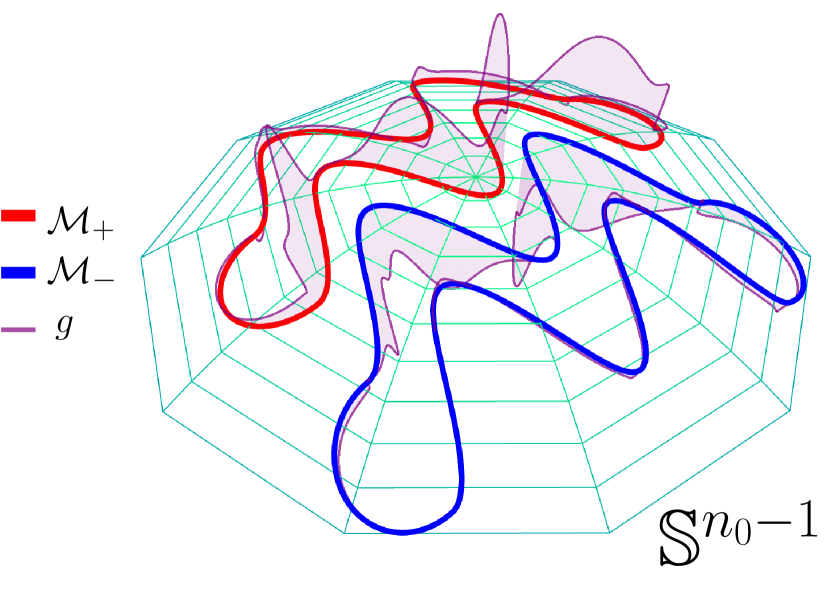
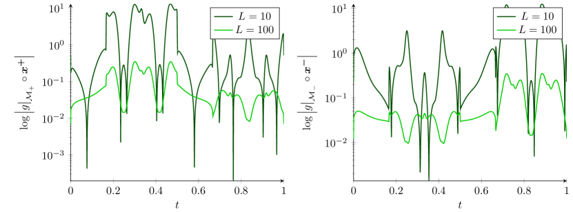
Figure 4: The effect of geometry and depth on the certificate. Left: The certificate $g$ computed numerically from the kernel $\Theta$ for depth $L=50$ (defined in 3.1) and the geometry from Figure 1 with a uniform density, graphed over the manifolds. Control of the norm of the certificate implies rapid progress of gradient descent, as reflected in Theorem 3.2. Comparing to Figure 1, we note that the certificate has large magnitude near the point of minimum distance between the two curves—this is suggestive of the way the geometry sets the difficulty of the fitting problem. Right: To visualize the certificate norm more precisely, we graph the log-magnitude of the certificate for kernels $\Theta$ of varying depth $L$, viewing them through the arc-length parameterizations $\bm{x}_{\sigma}$ for the curves (left: $\mathcal{M}_{+}$; right: $\mathcal{M}_{-}$). At a coarse scale, the maximum magnitude decreases as the depth increases; at a finer scale, curvature-associated defects are ‘smoothed out’. This indicates the role of depth as a fitting resource. See Appendix A for further experimental details.

The proof of Theorem 3.1 is novel, both in the context of kernel regression on manifolds and in the context of NTK-regime neural network training. We detail the key intuitions for the proof in Section 4. As suggested above, applying Theorem 3.1 to construct a certificate is straightforward: given a suitable setting of $L$ for a two curve problem instance, we obtain an approximate certificate $g$ via Theorem 3.1. Then with the triangle inequality and the Schwarz inequality, we can bound

$$\lVert\bm{\Theta}^{\mathrm{NTK}}_{\mu}[g]-\zeta_{0}\rVert_{L^{2}_{\mu}}\leq\lVert\bm{\Theta}_{\mu}^{\mathrm{NTK}}-\bm{\Theta}_{\mu}\rVert_{L^{2}_{\mu}\to L^{2}_{\mu}}\lVert g\rVert_{L^{2}_{\mu}}+\lVert\zeta_{0}-\zeta\rVert_{L^{2}_{\mu}}+\lVert\bm{\Theta}_{\mu}[g]-\zeta\rVert_{L^{2}_{\mu}},$$

and leveraging suitable probabilistic control (see Appendix G) of the approximation errors in the previous expression, as well as on $\lVert\zeta\rVert_{L^{2}_{\mu}}$, then yields bounds for the certificate problem. Applying the reductions from gradient descent dynamics in the NTK regime to certificates discussed in Section 2.1, we then obtain an end-to-end guarantee for the two curve problem.

Theorem 3.2 (Generalization).

Let $\mathcal{M}$ be two disjoint smooth, regular, simple closed curves, satisfying $\angle(\bm{x},\bm{x}^{\prime})\leq\pi/2$ for all $\bm{x},\bm{x}^{\prime}\in\mathcal{M}$. For any $0<\delta\leq 1/e$, choose $L$ so that

$$L \geq K\max\left\{\frac{1}{\left(\Delta\sqrt{1+\kappa^{2}}\right)^{C\text{{\char 86\relax}}(\mathcal{M})}},C_{\mu}\log^{9}(\tfrac{1}{\delta})\log^{24}(C_{\mu}n_{0}\log(\tfrac{1}{\delta})),e^{C^{\prime}\max\{\operatorname{len}(\mathcal{M})\hat{\kappa},\log(\hat{\kappa})\}},P\right\}$$

$$n =K^{\prime}L^{99}\log^{9}(1/\delta)\log^{18}(Ln_{0})$$

$$N \geq L^{10},$$

and fix $\tau>0$ such that $\frac{C^{\prime\prime}}{nL^{2}}\leq\tau\leq\frac{c}{nL}$. Then with probability at least $1-\delta$, the parameters obtained at iteration $\lfloor L^{39/44}/(n\tau)\rfloor$ of gradient descent on the finite sample loss yield a classifier that separates the two manifolds.

The constants $c,C,C^{\prime},C^{\prime\prime},K,K^{\prime}>0$ are absolute, and the constant $C_{\mu}$ is equal to $\frac{\max\{\rho_{\min}^{19},\rho_{\min}^{-19}\}(1+\rho_{\max})^{12}}{\left(\min\,\left\{\mu(\mathcal{M}_{+}),\mu(\mathcal{M}_{-})\right\}\right)^{11/2}}$. $P$ is a polynomial $\operatorname{poly}\{M_{3},M_{4},M_{5},\operatorname{len}(\mathcal{M}),\Delta^{-1}\}$ of degree at most $36$, with degree at most $12$ when viewed as a polynomial in $M_{3},M_{4},M_{5}$ and $\operatorname{len}(\mathcal{M})$, and of degree at most $24$ as a polynomial in $\Delta^{-1}$.

Theorem 3.2 represents the first end-to-end guarantee for training a deep neural network to classify a nontrivial class of low-dimensional nonlinear manifolds. We call attention to the fact that the hypotheses of Theorem 3.2 are completely self-contained, making reference only to intrinsic properties of the data and the architectural hyperparameters of the neural network (as well as $\operatorname{poly}(\log n_{0})$), and that the result is algorithmic, as it applies to training the network via constant-stepping gradient descent on the empirical square loss and guarantees generalization within $L^{2}$ iterations. Furthermore, Theorem 3.2 can be readily extended to the more general setting of regression on curves, given that we have focused on training with the square loss.

4 Proof Sketch

In this section, we provide an overview of the key elements of the proof of Theorem 3.1, where we show that the equation $\bm{\Theta}_{\mu}[g]\approx\zeta$ admits a solution $g$ (the certificate) of small norm. To solve the certificate problem for $\mathcal{M}$, we require a fine-grained understanding of the kernel $\Theta$. The most natural approach is to formally set $g=\sum_{i=1}^{\infty}\lambda_{i}^{-1}\langle\zeta,v_{i}\rangle_{L^{2}_{\mu}}v_{i}$ using the eigendecomposition of $\bm{\Theta}_{\mu}$ (just as constructed in Section 2.1 for $\bm{\Theta}_{\mu}^{\mathrm{NTK}}$), and then argue that this formal expression converges by studying the rate of decay of $\lambda_{i}$ and the alignment of $\zeta$ with eigenvectors of $\bm{\Theta}_{\mu}$; this is the standard approach in the literature [50, 57]. However, as discussed in Section 2.1, the nonlinear structure of $\mathcal{M}$ makes obtaining a full diagonalization for $\bm{\Theta}_{\mu}$ intractable, and simple asymptotic characterizations of its spectrum are insufficient to prove that the solution $g$ has small norm. Our approach will therefore be more direct: we will study the ‘spatial’ properties of the kernel $\Theta$ itself, in particular its rate of decay away from $\bm{x}=\bm{x}^{\prime}$, and thereby use the network depth $L$ as a resource to reduce the study of the operator $\bm{\Theta}_{\mu}$ to a simpler, localized operator whose invertibility can be proved using harmonic analysis. We will then use differentiability properties of $\Theta$ to transfer the solution obtained by inverting this auxiliary operator back to the operator $\bm{\Theta}_{\mu}$. We refer readers to Appendix E for the full proof.

We simplify the proceedings using two basic reductions. First, with a small amount of auxiliary argumentation, we can reduce from the study of the operator-with-density $\bm{\Theta}_{\mu}$ to the density-free operator $\bm{\Theta}$. Second, the kernel $\Theta(\mathbf{x},\mathbf{x}^{\prime})$ is a function of the angle $\angle(\mathbf{x},\mathbf{x}^{\prime})$, and hence is rotationally invariant. This kernel is maximized at $\angle(\mathbf{x},\mathbf{x}^{\prime})=0$ and decreases monotonically as the angle increases, reaching its minimum value at $\angle(\mathbf{x},\mathbf{x}^{\prime})=\pi$. If we subtract this minimum value, it should not affect our ability to fit functions, and we obtain a rotationally invariant kernel $\Theta^{\circ}(\mathbf{x},\mathbf{x}^{\prime})=\psi^{\circ}(\angle(\mathbf{x},\mathbf{x}^{\prime}))$ that is concentrated around angle $0$. In the following, we focus on certificate construction for the kernel $\Theta^{\circ}$. Both simplifications are justified in LABEL:sec:certificate_dc_density.

4.1 The Importance of Depth: Localization of the Neural Tangent Kernel

The first problem one encounters when attempting to directly establish (a property like) invertibility of the operator $\bm{\Theta}^{\circ}$ is its action across connected components of $\mathcal{M}$: the operator $\bm{\Theta}^{\circ}$ acts by integrating against functions defined on $\mathcal{M}=\mathcal{M}_{+}\cup\mathcal{M}_{-}$, and although it is intuitive that most of its image’s values on each component will be due to integration of the input over the same component, there will always be some ‘cross-talk’ corresponding to integration over the opposite component that interferes with our ability to apply harmonic analysis tools. To work around this basic issue (as well as others we will see below), our argument proceeds via a localization approach: we will exploit the fact that as the depth $L$ increases, the kernel $\Theta^{\circ}$ sharpens and concentrates around its value at $\bm{x}=\bm{x}^{\prime}$, to the extent that we can neglect its action across components of $\mathcal{M}$ and even pass to the analysis of an auxiliary localized operator. This reduction is enabled by new sharp estimates for the decay of the angle function $\psi^{\circ}$ that we establish in Section F.3. Moreover, the perspective of using the network depth as a resource to localize the kernel $\Theta^{\circ}$ and exploiting this to solve the classification problem appears to be new: this localization is typically presented as a deficiency in the literature (e.g. [51]).

At a more formal level, when the network is deep enough compared to geometric properties of the curves, for each point $\mathbf{x}$, the majority of the mass of the kernel $\Theta^{\circ}(\mathbf{x},\mathbf{x}^{\prime})$ is taken within a small neighborhood $d_{\mathcal{M}}(\mathbf{x},\mathbf{x}^{\prime})\leq r$ of $\mathbf{x}$. When $d_{\mathcal{M}}(\mathbf{x},\mathbf{x}^{\prime})$ is small relative to $\kappa$, we have $d_{\mathcal{M}}(\mathbf{x},\mathbf{x}^{\prime})\approx\angle(\mathbf{x},\mathbf{x}^{\prime})$. This allows us to approximate the local component by the following invariant operator:

$$\widehat{\mathbf{M}}[f](\mathbf{x}_{\sigma}(s))=\int_{s^{\prime}=s-r}^{s+r}\psi^{\circ}(\lvert s-s^{\prime}\rvert)f(\mathbf{x}_{\sigma}(s^{\prime}))ds^{\prime}.$$ (4.1)

This approximation has two main benefits: (i) the operator $\widehat{\mathbf{M}}$ is defined by intrinsic distance $s^{\prime}-s$, and (ii) it is highly localized. In fact, (4.1) takes the form of a convolution over the arc length parameter $s$. This implies that $\widehat{\mathbf{M}}$ diagonalizes in the Fourier basis, giving an explicit characterization of its eigenvalues and eigenvectors. Moreover, because $\widehat{\mathbf{M}}$ is localized, the eigenvalues corresponding to slowly oscillating Fourier basis functions are large, and $\widehat{\mathbf{M}}$ is stably invertible over such functions. Both of these benefits can be seen as consequences of depth: depth leads to localization, which facilitates approximation by $\widehat{\mathbf{M}}$, and renders that approximation invertible over low-frequency functions. In our proofs, we will work with a subspace $S$ spanned by low-frequency basis functions that are nearly constant over a length $2r$ interval (this subspace ends up having dimension proportional to $1/r$; see Section C.3 for a formal definition), and use Fourier arguments to prove invertibility of $\widehat{\bm{M}}$ over $S$ (see Lemma E.6).

4.2 Stable Inversion over Smooth Functions

Our remaining task is to leverage the invertibility of $\widehat{\mathbf{M}}$ over $S$ to argue that $\mathbf{\Theta}$ is also invertible. In doing so, we need to account for the residual $\mathbf{\Theta}-\widehat{\mathbf{M}}$. We accomplish this directly, using a Neumann series argument: when setting $r\lesssim L^{-1/2}$ and the dimension of the subspace $S$ proportional to $1/r$, the minimum eigenvalue of $\widehat{\mathbf{M}}$ over $S$ exceeds the norm of the residual operator $\mathbf{\Theta}^{\circ}-\widehat{\mathbf{M}}$ (Lemma E.2). This argument leverages a decomposition of the domain into “near”, “far” and “winding” pieces, whose contribution to $\mathbf{\Theta}^{\circ}$ is controlled using the curvature, angle injectivity radius and 🍀-number (LABEL:lem:near_ub, LABEL:lem:winding_ub, LABEL:lem:far_ub). This guarantees the strict invertibility of $\mathbf{\Theta}^{\circ}$ over the subspace $S$, and yields a unique solution $g_{S}$ to the restricted equation $\mathbf{P}_{S}\mathbf{\Theta}^{\circ}[g_{S}]=\zeta$ (Theorem E.1).

This does not yet solve the certificate problem, which demands near solutions to the unrestricted equation $\mathbf{\Theta}^{\circ}[g]=\zeta$. To complete the argument, we set $g=g_{S}$ and use harmonic analysis considerations to show that $\mathbf{\Theta}^{\circ}[g]$ is very close to $S$. The subspace $S$ contains functions that do not oscillate rapidly, and hence whose derivatives are small relative to their norm (LABEL:lem:fourier_deriv_lb). We prove that $\mathbf{\Theta}^{\circ}[g]$ is close to $S$ by controlling the first three derivatives of $\mathbf{\Theta}^{\circ}[g]$, which introduces dependencies on $M_{1},\cdots,M_{5}$ in the final statement of our results (LABEL:lem:Theta_Sperp_proj). In controlling these derivatives, we leverage the assumption that $\sup_{\bm{x},\bm{x}^{\prime}\in\mathcal{M}}\angle(\bm{x},\bm{x}^{\prime})\leq\pi/2$ to avoid issues that arise at antipodal points—we believe the removal of this constraint is purely technical, given our sharp characterization of the decay of $\psi^{\circ}$ and its derivatives. Finally, we move from $\mathbf{\Theta}^{\circ}$ back to $\mathbf{\Theta}$ by combining near solutions to $\mathbf{\Theta}^{\circ}[g]=\zeta$ and $\mathbf{\Theta}^{\circ}[g_{1}]=1$, and iterating the construction to reduce the approximation error to an acceptable level (LABEL:sec:certificate_dc_density).

5 Discussion

A role for depth.

In the setting of fitting functions on the sphere $\mathbb{S}^{n_{0}-1}$ in the NTK regime with unstructured (e.g., uniformly random) data, it is well-known that there is very little marginal benefit to using a deeper network: for example, [63, 36, 50] show that the risk lower bound for RKHS methods is nearly met by kernel regression with a $2$-layer network’s NTK in an asymptotic ($n_{0}\to\infty$) setting, and results for fitting degree-$1$ functions in the nonasymptotic setting [56] are suggestive of a similar phenomenon. In a similar vein, fitting in the NTK regime with a deeper network does not change the kernel’s RKHS [46, 49, 45], and in a certain “infinite-depth” limit, the corresponding NTK for networks with ReLU activations, as we consider here, is a spike, guaranteeing that it fails to generalize [54, 51]. Our results are certainly not in contradiction to these facts—we consider a setting where the data are highly structured, and our proofs only show that an appropriate choice of the depth relative to this structure is sufficient to guarantee generalization, not necessary—but they nonetheless highlight an important role for the network depth in the NTK regime that has not been explored in the existing literature. In particular, the localization phenomenon exhibited by the deep NTK is completely inaccessible by fixed-depth networks, and simultaneously essential to our arguments to proving Theorem 3.2, as we have described in Section 4. It is an interesting open problem to determine whether there exist low-dimensional geometries that cannot be efficiently separated without a deep NTK, or whether the essential sufficiency of the depth-two NTK persists.

Closing the gap to real networks and data.

Theorem 3.2 represents an initial step towards understanding the interaction between neural networks and data with low-dimensional structure, and identifying network resource requirements sufficient to guarantee generalization. There are several important avenues for future work. First, although the resource requirements in Theorem 3.1, and by extension Theorem 3.2, reflect only intrinsic properties of the data, the rates are far from optimal—improvements here will demand a more refined harmonic analysis argument beyond the localization approach we take in Section 4.1. A more fundamental advance would consist of extending the analysis to the setting of a model for image data, such as cartoon articulation manifolds, and the NTK of a convolutional neural network with architectural settings that impose translation invariance [29, 39]—recent results show asymptotic statistical efficiency guarantees with the NTK of a simple convolutional architecture, but only in the context of generic data [64]. The approach to certificate construction we develop in Theorem 3.1 will be of use in establishing guarantees analogous to Theorem 3.2 here, as our approach does not require an explicit diagonalization of the NTK. In addition, extending our certificate construction approach to smooth manifolds of dimension larger than one is a natural next step. We believe our localization argument generalizes to this setting: as our bounds for the kernel $\psi$ are sharp with respect to depth and independent of the manifold dimension, one could seek to prove guarantees analogous to Theorem 3.1 with a similar subspace-restriction argument for sufficiently regular manifolds, such as manifolds diffeomorphic to spheres, where the geometric parameters of Section 2.2 have natural extensions. Such a generalization would incur at best an exponential dependence of the network on the manifold dimension for localization in high dimensions.

More broadly, the localization phenomena at the core of our argument appear to be relevant beyond the regime in which the hypotheses of Theorem 3.2 hold: we provide a preliminary numerical experiment to this end in Section A.3. Training fully-connected networks with gradient descent on a simple manifold classification task, low training error appears to be easily achievable only when the decay scale of the kernel is small relative to the inter-manifold distance even at moderate depth and width, and this decay scale is controlled by the depth of the network.

.tocmtappendix mtchapternone mtappendixsubsection

Appendix A Details of Figures

A.1 Figure 3

🍀-number experiment.

In each panel, the two curves are projection of curves $\bm{x}_{+}:[0,2\pi]\to\mathbb{S}^{3}$ and $\bm{x}_{-}:[0,2\pi]\to\mathbb{S}^{3}$. We actually generate the curves as shown in the figure (i.e., in a three-dimensional space), then map them to the sphere using the map $(u,v,w)\mapsto(u,v,w,\sqrt{1-u^{2}-v^{2}-w^{2}})$. In this three-dimensional space, the top left panel’s blue curve (denoted $\bm{x}_{-}$ henceforth) and each panel’s red curve (denoted $\bm{x}_{+}$ henceforth, and which is the same for all panels) are defined by the parametric equations

$$\left(\begin{array}[]{c}x_{-,1}(t)\\ x_{-,2}(t)\\ x_{-,3}(t)\end{array}\right) = \left(\begin{array}[]{c}\cos(4t)\\ \cos\left(\frac{\pi}{8}\right)\cos(t)\left(\sin(4t)+1+\delta\right)+\sin\left(\frac{\pi}{8}\right)\sin(t)\left(\sin(4t)+1+\delta\right)\\ -\sin\left(\frac{\pi}{8}\right)\cos(t)\left(\sin(4t)+1+\delta\right)+\cos\left(\frac{\pi}{8}\right)\sin(t)\left(\sin(4t)+1+\delta\right)\end{array}\right)$$

$$\left(\begin{array}[]{c}x_{+,1}(t)\\ x_{+,2}(t)\\ x_{+,3}(t)\end{array}\right) = \left(\begin{array}[]{c}4\sin(t)\\ 4\left(\cos(t)-1\right)\\ 0\end{array}\right),$$

where $\delta$ sets the separation between the manifolds and is set here to $\delta=0.05$. We then rescale both curves by a factor $.01$: the scale of the curves is chosen such that the curvature of the sphere has a negligible effect on the curvature of the manifolds (since the chart mapping we use here distorts the curves more nearer to the boundary of the unit disk $\{(u,v,w)\nonscript\>|\allowbreak\nonscript\>\mathopen{}u^{2}+v^{2}+w^{2}\leq 1\}$).

From here, we use an “unfolding” process to obtain the blue curves in the other three panels from $\bm{x}_{-}$. To do this, points where $|\frac{\mathrm{d}x_{-,2}}{\mathrm{d}t}|=|\frac{\mathrm{d}x_{-,3}}{\mathrm{d}t}|$ are found numerically. There are $8$ such points in total, and parts of the curve between pairs of these points are reflected across the line defined by such a pair in the $(x_{2},x_{3})$ plane. This can be done for any number of pairs between $1$ and $4$, generating the curves shown. This procedure ensures that aside from the set of $8$ points, the curvature at every point along the curve is preserved and there is no discontinuity in the first derivative, while making the geometries loop back to the common center point more. For an additional visualization of the geometry, see Figure 5.

\begin{overpic}[width=433.62pt]{./figures/slinky_full.pdf} \put(90.0,35.2){$\text{{\char 86\relax}}=1$} \put(90.0,41.4){$\text{{\char 86\relax}}=2$} \put(90.0,47.6){$\text{{\char 86\relax}}=3$} \put(90.0,53.8){$\text{{\char 86\relax}}=4$} \put(90.0,60.5){$\mathcal{M}_{+}$} \end{overpic}

Figure 5: The two curve geometry described in Section A.1. The different choices of $\mathcal{M}_{-}$ that lead to different 🍀-number are overlapping. The legend indicates the 🍀-number of the two curves problem obtained by considering the same $\mathcal{M}_{+}$ but a different $\mathcal{M}_{-}$ as indicated by the color.

Given these geometries, in order to compute the certificate norm for the experiment in the top-right panel, we evaluate the resulting curves at $200$ points each, chosen by picking equally spaced points in $[0,2\pi]$ and evaluating the parametric equations. The certificate itself is evaluated numerically as in Section A.2.

Rotated MNIST digits.

We rotate an MNIST image around its center by $i*\pi/100$ for integer $i$ between $0$ and $199$. We then apply t-SNE [9] using the scikit-learn package with perplexity $20$ to generate the embeddings.

A.2 Figure 4

We give full implementation details for this figure here, mixed with conceptual ideas that underlie the implementation. The manifolds $\mathcal{M}_{+}$ and $\mathcal{M}_{-}$ are defined by parametric equations $\bm{x}_{+}:[0,1]\to\mathbb{S}^{2}$ and $\bm{x}_{-}:[0,1]\to\mathbb{S}^{2}$; it is not practical to obtain unit-speed parameterizations of general curves, so we also have parametric equations for their derivatives $\dot{\bm{x}}_{\sigma}:[0,1]\to\mathbb{R}^{2}$. These are important in our setting since for non-unit-speed curves, the chain rule gives for the integral of a function (say) $f:\mathcal{M}_{+}\to\mathbb{R}$

$$\int_{\mathcal{M}_{+}}f(\bm{x})\mathop{}\!\mathrm{d}\bm{x}=\int_{[0,1]}(f\circ\bm{x}_{+}(t))\lVert\dot{\bm{x}}_{+}(t)\rVert_{2}\mathop{}\!\mathrm{d}t.$$

In particular, in our experiments, we want to work with a uniform density $\rho=(\rho_{+},\rho_{-})$ on the manifolds, where the classes are balanced. To achieve this, use the previous equation to get that we require

$$1 =\int_{\mathcal{M}_{+}}\rho_{+}(\bm{x})\mathop{}\!\mathrm{d}\bm{x}+\int_{\mathcal{M}_{-}}\rho_{-}(\bm{x})\mathop{}\!\mathrm{d}\bm{x}$$

$$=\int_{\mathcal{M}_{+}}(\rho_{+}\circ\bm{x}_{+})(t)\lVert\dot{\bm{x}}_{+}(t)\rVert_{2}\mathop{}\!\mathrm{d}t+\int_{\mathcal{M}_{-}}(\rho_{-}\circ\bm{x}_{-})(t)\lVert\dot{\bm{x}}_{-}(t)\rVert_{2}\mathop{}\!\mathrm{d}t.$$

A uniform density on $\mathcal{M}$ is not a constant value—rather, it is characterized by being translation-invariant. It follows that $\rho_{\sigma}$ should be defined by

$$\rho_{\sigma}\circ\bm{x}_{\sigma}(t)=\frac{1}{2\lVert\dot{\bm{x}}_{\sigma}(t)\rVert_{2}}.$$

For the experiment, we solve a discretization of the certificate problem, for which the above ideas will be useful. Consider $\Theta$ in 3.1 for a fixed depth $L$ (and $n=2$, since width is essentially irrelevant here). By the above discussion, the certificate problem in this setting is to solve for the certificate $g=(g_{+},g_{-})$

$$f_{\star}=\frac{1}{2}\left(\int_{[0,1]}\Theta(\,\cdot\,,\bm{x}_{+}(t))g_{+}\circ\bm{x}_{+}(t)\mathop{}\!\mathrm{d}t+\int_{[0,1]}\Theta(\,\cdot\,,\bm{x}_{-}(t))g_{-}\circ\bm{x}_{-}(t)\mathop{}\!\mathrm{d}t\right).$$

Here, we have eliminated the initial random neural network output $f_{\bm{\theta}_{0}}$ from the RHS. Aside from making computation easier, this is motivated by fact that the network output is approximately piecewise constant for large depth $L$, and we therefore expect it not to play much of a role here. Let $M\in\mathbb{N}$ denote the discretization size. Then a finite-dimensional approximation of the previous integral equation is given by the linear system

$$f_{\star}\circ\bm{x}_{\sigma}(t_{i})=\frac{1}{2M}\left(\sum_{j=1}^{M}\Theta(\bm{x}_{\sigma}(t_{i}),\bm{x}_{+}(t_{j}))g_{+}\circ\bm{x}_{+}(t_{j})+\sum_{j=1}^{M}\Theta(\bm{x}_{\sigma}(t_{i}),\bm{x}_{-}(t_{j}))g_{-}\circ\bm{x}_{-}(t_{j})\right)$$ (A.1)

for all $i\in[M]$ and $\sigma\in\{\pm 1\}$, and where $t_{i}=(i-1)/M$. Of course, $f_{\star}\circ\bm{x}_{\sigma}(t)=\sigma$, so the equation simplifies further, and because the kernel $\Theta$ and this target $f_{\star}$ are smooth, there is a convergence of the data in this linear system in a precise sense to the data in the original integral equation as $M\to\infty$. In particular, define a matrix $\bm{T}^{+}$ by $T^{+}_{ij}=\Theta(\bm{x}_{+}(t_{i}),\bm{x}_{+}(t_{j}))$, define a matrix $\bm{T}^{-}$ by $T^{-}_{ij}=\Theta(\bm{x}_{-}(t_{i}),\bm{x}_{-}(t_{j}))$, and define a matrix $\bm{T}^{\pm}$ by $T^{\pm}_{ij}=\Theta(\bm{x}_{+}(t_{i}),\bm{x}_{-}(t_{j}))$, all of size $M\times M$. Then the $2M\times 2M$ linear system

$$\begin{bmatrix}\mathbf{1}\\ -\mathbf{1}\end{bmatrix}=\frac{1}{2M}\begin{bmatrix}\bm{T}^{+}&\bm{T}^{\pm}\\ \left(\bm{T}^{\pm}\right)^{\ast}&\bm{T}^{-}\end{bmatrix}\begin{bmatrix}\bm{g}_{+}\\ \bm{g}_{-}\end{bmatrix}$$ (A.2)

is equivalent to the discretization in A.1. We implement and solve the system in A.2 using the definitions we have given above, using the pseudoinverse of the $2M\times 2M$ matrix appearing in this expression to obtain $[\bm{g}_{+},\bm{g}_{-}]^{\ast}$, and plot the results in Figure 4, in particular interpreting $(\bm{g}_{\sigma})_{i}$ as the sampled point $g_{\sigma}\circ\bm{x}_{\sigma}(t_{i})$ as in A.1 when we plot in the left panel of Figure 4. Evidently, it would be immediate to modify the experiment to replace the LHS of A.1 by the error $f_{\bm{\theta}_{0}}-f_{\star}$: the same protocol given above would work, but there would be an element of randomness added to the experiments.

Specifically, in Figure 4 we set $M=900$. When plotting the solution to A.2, i.e. the vector $[\bm{g}_{+},\bm{g}_{-}]^{\ast}$, we moreover scale the vector by a factor of $0.3$ to facilitate visualization.

A.3 Kernel Decay Scale and Trainability of Realisting Networks: Empirical Evidence

\begin{overpic}[width=303.53267pt]{figures/training_error_varying_delta} \put(102.0,58.0){\rotatebox{270.0}{Log Training Error}} \put(15.0,-32.0){\framebox(0.0,0.0)[bl]{\includegraphics[scale={.5}]{figures/curves_delta_0p9.pdf}}} \put(51.0,-32.0){\framebox(0.0,0.0)[bl]{\includegraphics[scale={.5}]{figures/curves_delta_0p3.pdf}}} \par\put(15.0,65.0){ \leavevmode\hbox to28.45pt{\vbox to2.85pt{\text{[drawing]}}}} \put(19.0,-7.7){ \leavevmode\hbox to36.99pt{\vbox to35.57pt{\text{[drawing]}}}} \put(64.0,-7.7){ \leavevmode\hbox to36.99pt{\vbox to35.57pt{\text{[drawing]}}}} \put(27.0,65.0){{\color[rgb]{1,1,1}{$\psi^{\circ}$ Decay Scale}}} \end{overpic}

Figure 6: The decay properties of the NTK are predictive of trainability on a toy dataset. We plot the log training error of networks of varying depth that are trained to classify two curves with varying separation. The insets show a projection of the geometry onto the plane for separation values $0.3$ and $0.9$. For each depth $L$, the characteristic decay scale of the DC-subtracted NTK ($\psi^{\circ}$) is computed numerically and plotted in green. We find that small training loss is only achievable if the decay scale of the kernel is small compared to the inter-manifold distance, hence the decay scale is predictive of trainability.

One of the main insights into the manifold classification problem that is utilized to obtain Theorem 3.2 is that (roughly speaking) the depth of a fully-connected network controls the decay properties of the network’s NTK, and that fitting can be guaranteed once the decay occurs on a spatial scale that is small relative to certain geometric properties of the data. Here we provide empirical evidence that this phenomenon holds beyond the regime in which our main theorems hold, and in fact is relevant for networks of moderate width and depth as well.

We draw $400$ samples each from a uniform distribution over a union of two curves that are related by a rotation by a geodesic angle that is varied from $0.2$ to $1.0$ in increments of $0.1$. The curves are not linearly separable even for large angle (see insets in Fig. 6). These curves are embedded in $\mathbb{S}^{n_{0}-1}$ for $n_{0}=128$ and subjected to a rotation drawn uniformly from the Haar measure. We then train a fully-connected network to classify the curves using $\ell^{2}$ loss. The network has width $n=256$ and we vary the depth from $L=2$ to $L=10$, and train using full-batch gradient descent for $10^{5}$ iterations with learning rate $\tau=1/(4nL)$ (so that the total effective "training time" is independent of depth). We plot the log training error after training as a function of depth and the inter-manifold distance. For each depth $L$, we estimate an effective “decay scale” of the DC-subtracted skeleton $\psi^{\circ}$ by determining the point $s^{\star}$ such that $\psi^{\circ}(s^{\star})=\frac{\psi^{\circ}(0)}{2}$.

The results are presented in Fig. 6. We observe that the network convergences to small training loss only when the depth is large comparable to the inverse of the manifold separation. As the depth represents the decay rate of the NTK, this indicates that a deeper network generates a localized NTK, allowing faster decay of the training error and making the classification problem easy. Notice that since the geometry of the dataset and network architecture do not satisfy all the assumptions of Theorem 3.2, the experiment provides evidence that the underlying phenomena regarding the role of the depth hold in greater generality. This preliminary result also suggests that the connection between the network architecture and the data geometry, as expressed through the decay properties of the NTK, can have a dramatic effect on the training process even for fully-connected networks.

Appendix B Notation

We use bold lowercase $\mathbf{x}$ for vectors and uppercase $\mathbf{A}$ for matrices and operators. We generally use non-bold notation to represent scalars and scalar-valued functions. $\mathbb{R},\mathbb{C},\mathbb{Z}$ are used for the real numbers, complex numbers and integers, respectively. $\mathbb{N}_{0}$ represents non-negative integers, and $\mathbb{N}$ represents the natural numbers. $\mathbb{R}^{n}$ represents $n$-dimensional Euclidean space, $\mathbb{C}^{n}$ represents the space of complex $n$-tuples (as a $n$-dimensional vector space over $\mathbb{C}$) and $\mathbb{S}^{n-1}\subset\mathbb{R}^{n}$ represents the $n-1$ dimensional sphere centered at zero with unit radius. For a complex number $z=x+iy$ (or a complex-valued function), $\lvert z\rvert=\sqrt{x^{2}+y^{2}}$ denotes the complex modulus, and $\mkern 1.5mu\overline{\mkern-1.5muz\mkern-1.5mu}\mkern 1.5mu=x-iy$ denotes the complex conjugate. For $\bm{x},\bm{y}\in\mathbb{C}^{n}$, we denote $\lVert\mathbf{x}\rVert_{p}=\left(\sum_{i=1}^{n}\lvert x_{i}\rvert^{p}\right)^{1/p}$ as the $p$-norm and $\langle\bm{x},\bm{y}\rangle=\sum_{i=1}^{n}\mkern 1.5mu\overline{\mkern-1.5mux\mkern-1.5mu}\mkern 1.5mu_{i}y_{i}$ as the standard (second-argument-linear) inner product. We use $\mathbf{x}^{*}$ and $\mathbf{A}^{*}$ to represent the conjugate transpose of vectors or matrices of complex numbers (so e.g. $\bm{x}^{\ast}\bm{y}=\langle\bm{x},\bm{y}\rangle$). We use $\mathbf{P}_{S}$ to represent the orthogonal projection operator onto a closed subspace $S$ of a normed vector space (typically a Hilbert space).

For a Borel measure space $(X,\mu)$ and any measurable function $f:X\to\mathbb{C}$, we use $\lVert f\rVert_{L^{p}_{\mu}}=\linebreak(\int_{\mathbf{x}\in X}\lvert f(\mathbf{x})\rvert^{p}d\mu(\mathbf{x}))^{1/p}$ to represent the $L^{p}$ norm of $f$ for $0<p<\infty$. We omit the measure from the notation when it is clear from context. For $p=\infty$, we use $\lVert f\rVert_{L^{\infty}_{\mu}}=\inf\{C\geq 0\nonscript\>|\allowbreak\nonscript\>\mathopen{}\lvert f(\mathbf{x})\rvert\leq C\text{ for $\mu$-almost every $\mathbf{x}$}\}$ to represent its essential supremum. We denote the $L^{p}$ space of $(X,\mu)$ by $L^{p}_{\mu}(X)$ (or simply $L^{p}_{\mu}$ when the space is clear from context), which is formed by all complex-valued measurable functions with finite $L^{p}_{\mu}$ norm. For another space $(Y,\nu)$ and a (linear) operator $\bm{T}:L^{p}_{\mu}(X)\to L^{q}_{\nu}(Y)$, we represent its $L_{\mu}^{p}\to L_{\nu}^{q}$ operator norm as $\lVert\bm{T}\rVert_{L_{\mu}^{p}\to L_{\nu}^{q}}=\sup_{\lVert f\rVert_{L^{p}_{\mu}}=1}\lVert\bm{T}[f]\rVert_{L^{q}_{\nu}}$. When $X=Y$, $\mu=\nu$, and $p=q=2$ (and $(X,\mu)$ is sufficiently regular), we have a Hilbert space; we write $\langle f,g\rangle_{L^{2}_{\mu}}=\int_{X}\bar{f}(\bm{x})g(\bm{x})\mathop{}\!\mathrm{d}\mu(\bm{x})$ for the inner product, and $\bm{T}^{\ast}$ to denote the associated adjoint of an operator $\bm{T}$ (so e.g. $f^{\ast}=\langle f,\>\cdot\>\rangle$ denotes the corresponding dual element of a function $f$). We use $\operatorname{\mathrm{Id}}:L_{\mu}^{p}(X)\to L_{\mu}^{p}(X)$ to denote the identity operator, i.e. $\operatorname{\mathrm{Id}}[f]=f$ for every $f\in L^{p}_{\mu}$. For $S\subset X$, we use $\mathbbm{1}_{S}$ to represent the indicator function $\mathbbm{1}_{S}(\mathbf{x})=1,\forall\mathbf{x}\in S$ and $0$ otherwise; we will write $\mathbbm{1}$ to denote $\mathbbm{1}_{X}$. For a map $\varphi:X\to X$ and $i\in N$, we use $\varphi^{[i]}$ to denote its $i$-th fold iterated composition of itself, i.e. $\varphi^{[i]}(\mathbf{x})=\varphi\left(\varphi^{(i-1)}(\mathbf{x})\right)$. For $i\in N$, $f^{(i)}$ is normally used to represent a function of a real variable $f$’s $i$-th order derivatives. For example, when the space is a two curve problem instance $\mathcal{M}$, if $\mathbf{h}:\mathcal{M}\to\mathbb{C}^{n}$, we define its derivatives $\mathbf{h}^{(i)}$ in C.5; for a kernel $\Theta:\mathcal{M}\times\mathcal{M}\to\mathbb{R}$, we define its derivatives along the curve in LABEL:def:deriv-R.

For a Borel measure space $(X,\mu)$, a kernel $K$ is a mapping $K:X\times X\to\mathbb{R}$. We use $\mathbf{K}$ for its associated Fredholm integral operator. In other words, for measurable function $f$ we have $\mathbf{K}_{\mu}[g](\mathbf{x})=\int_{\mathbf{x}^{\prime}\in X}K(\mathbf{x},\mathbf{x}^{\prime})f(\mathbf{x}^{\prime})\mathop{}\!\mathrm{d}\mu(\mathbf{x}^{\prime})$. When $X$ is a Riemannian manifold, an omitted subscript/measure will always denote the Riemannian measure.

We use both lowercase and uppercase letters $c,C$ for absolute constants whose value are independent of all parameters and $c_{\tau}$, $C_{\tau}$ for numbers whose value only depend on some parameter $\tau$. Throughout the text, $c$ is used to represent numbers whose value should be small while $C$ is for those whose value should be large. We use $C_{1},C_{2},\dots$ for constants whose values are fixed within a proof while values of $C,C^{\prime},C^{\prime\prime},\dots$ may change from line to line.

Appendix C Key Definitions

C.1 Problem Formulation

The contents of this section will mirror Section 2.1, but provide additional technical details that were omitted there for the sake of concision and clarity of exposition. In this sense, we will focus on a rigorous formulation of the problem here, rather than on intuition: we encourage the reader to consult Section 2.1 for a more conceptually-oriented problem formulation. As in Section 2.1, we acknowledge that much of this material follows the technical exposition of [61].

Adopting the model proposed in [61], we let $\mathcal{M}_{+},\mathcal{M}_{-}$, denote two class manifolds, each a smooth, regular, simple closed curve in $\mathbb{S}^{n_{0}-1}$, with ambient dimension $n_{0}\geq 3$. We further assume $\mathcal{M}$ precludes antipodal points by asking

$$\angle(\mathbf{x},\mathbf{x}^{\prime})\leq\pi/2,\quad\forall\mathbf{x},\mathbf{x}^{\prime}\in\mathcal{M}.$$ (C.1)

We denote $\mathcal{M}=\mathcal{M}_{+}\cup\mathcal{M}_{-}$, and the data measure supported on $\mathcal{M}$ as $\mu$. We assume that $\mu$ admits a density $\rho$ with respect to the Riemannian measure on $\mathcal{M}$, and that this density is bounded from below by some $\rho_{\min}>0$. We will also write $\rho_{\max}=\sup_{\bm{x}\in\mathcal{M}}\rho(\bm{x})$. For background on curves and manifolds, we refer the reader to to [10, 27].

Given $N$ i.i.d. samples $(\mathbf{x}_{1},\cdots,\mathbf{x}_{N})$ from $\mu$ and their labels, given by the labeling function $f_{\star}:\mathcal{M}\to\{\pm 1\}$ defined by

$$f_{\star}(\bm{x})=\begin{cases}+1&\bm{x}\in\mathcal{M}_{+}\\ -1&\bm{x}\in\mathcal{M}_{-},\end{cases}$$

we train a fully-connected network with ReLU activations and $L$ hidden layers of width $n$ and scalar output. We will write $\bm{\theta}=(\bm{W}^{1},\dots,\bm{W}^{L+1})$ to denote an abstract set of admissible parameters for such a network; concretely, the features at layer $\ell\in\{1,2,\dots,L\}$ with parameters $\bm{\theta}$ and input $\bm{x}$ are written as $\bm{\alpha}_{\bm{\theta}}^{\ell}(\bm{x})=\left[\mathbf{W}^{\ell}\bm{\alpha}_{\bm{\theta}}^{\ell-1}(\bm{x})\right]_{+}$, where $[x]_{+}=\max\{x,0\}$ denotes the ReLU (and we adopt in general the convention of writing $[\bm{x}]_{+}$ to denote application of the scalar function $[\>\cdot\>]_{+}$ to each entry of the vector $\bm{x}$), with boundary condition $\bm{\alpha}_{\bm{\theta}}^{0}(\bm{x})=\bm{x}$, and the network output on an input $\bm{x}$ is written $f_{\bm{\theta}}(\bm{x})=\mathbf{W}^{L+1}\bm{\alpha}_{\bm{\theta}}^{L}(\bm{x})$. We will also write $\zeta_{\bm{\theta}}(\bm{x})=f_{\bm{\theta}}(\bm{x})-f_{\star}(\bm{x})$ to denote the fitting error. We use Gaussian initialization: if $\ell\in\{1,2,\dots,L\}$, the weights are initialized as $W_{ij}^{\ell}\sim_{\mathrm{i.i.d.}}\mathcal{N}(0,\frac{2}{n})$, and the top level weights are initialized as $W_{i}^{L+1}\sim_{\mathrm{i.i.d.}}\mathcal{N}(0,1)$ in order to preserve the expected feature norm. In the sequel, we will write $\bm{\theta}_{0}$ to denote the collection of these initial random parameters, and therefore $f_{\bm{\theta}_{0}}$ to denote the initial random network.

We will employ a convenient “empirical measure” notation to concisely represent finite-sample and population quantities in the analysis. Let $\mu^{N}=\frac{1}{N}\sum_{i=1}^{N}\delta_{\{\bm{x}_{i}\}}$ denote the empirical measure associated to our i.i.d. random sample from the population measure $\mu$, where $\delta_{\bm{p}}$ denotes a Dirac measure at a point $\bm{p}$. We train on the square loss $\mathcal{L}_{\mu^{N}}(\bm{\theta})=(1/2)\int_{\mathcal{M}}\left(\zeta_{\bm{\theta}}(\bm{x})\right)^{2}\mathop{}\!\mathrm{d}\mu^{N}(\bm{x})$ (of course one simply has $\mathcal{L}_{\mu^{N}}(\bm{\theta})=1/(2N)\sum_{i=1}^{N}\left(\zeta_{\bm{\theta}}(\bm{x}_{i})\right)^{2}$), which we minimize using randomly-initialized “gradient descent” starting at $\bm{\theta}_{0}$ with constant step size $\tau>0$. We put gradient descent in quotations here because the loss $\mathcal{L}_{\mu^{N}}$ is only almost-everywhere differentiable, due to the nondifferentiability of the ReLU activation $[\>\cdot\>]_{+}$: in this sense our algorithm for minimization is ‘gradient-like’, in that it corresponds to a gradient descent iteration at almost all values of the parameters. Concretely, we define

$$\bm{\beta}^{\ell}_{\bm{\theta}}(\bm{x})=\left(\bm{W}^{L+1}\bm{P}_{I_{L}(\bm{x})}\bm{W}^{L}\bm{P}_{I_{L-1}(\bm{x})}\dots\bm{W}^{\ell+2}\bm{P}_{I_{\ell+1}(\bm{x})}\right)^{\ast}$$

for $\ell=0,1,\dots,L-1$, where

$$I_{\ell}(\bm{x})=\left\{i\in[n]\nonscript\>\middle|\allowbreak\nonscript\>\mathopen{}\left\langle\bm{e}_{i},\bm{\alpha}^{\ell}_{\bm{\theta}}(\bm{x})\right\rangle>0\right\},\qquad\bm{P}_{I_{\ell}(\bm{x})}=\sum_{i\in I_{\ell}(\bm{x})}\bm{e}_{i}\bm{e}_{i}^{\ast}$$

denotes the orthogonal projection onto the set of coordinates where the $\ell$-th activation at input $\bm{x}$ is positive (above, $\bm{e}_{i}$ denotes the $i$-th canonical basis vector, having its $j$-th entry equal to $1$ if $j=i$ and $0$ otherwise). Then we define ‘formal gradients’ of the network output with respect to the parameters (denoted by an operator $\widetilde{\nabla}$) by

$$\widetilde{\nabla}_{\bm{W}^{\ell}}f_{\bm{\theta}}(\bm{x})=\bm{\beta}^{\ell-1}_{\bm{\theta}}(\bm{x})\bm{\alpha}^{\ell-1}_{\bm{\theta}}(\bm{x})^{\ast}$$

for $\ell\in[L]$, and

$$\widetilde{\nabla}_{\bm{W}^{L+1}}f_{\bm{\theta}}(\bm{x})=\bm{\alpha}^{L}_{\bm{\theta}}(\bm{x})^{\ast}.$$

As stated above, these expressions agree with the actual gradients at points of differentiability (to see this, apply the chain rule). We then define a formal gradient of $\mathcal{L}_{\mu^{N}}$ by

$$\widetilde{\nabla}\mathcal{L}_{\mu^{N}}(\bm{\theta})=\int_{\mathcal{M}}\widetilde{\nabla}f_{\bm{\theta}}(\bm{x})\zeta_{\bm{\theta}}(\bm{x})\mathop{}\!\mathrm{d}\mu^{N}(\bm{x}).$$

Thus, our gradient-like algorithm we study here is given by the sequence of parameters $\bm{\theta}_{k+1}=\bm{\theta}_{k}-\tau\widetilde{\nabla}\mathcal{L}_{\mu^{N}}(\bm{\theta}_{k})$, with $\bm{\theta}_{0}$ given by the Gaussian initialization we describe above.

Our study of this gradient-like iteration is facilitated by using kernel regime techniques, which we will describe now. Formally, the gradient descent iteration implies the following “error dynamics” equation:

$$\zeta_{\bm{\theta}^{N}_{k+1}}(\bm{x})=\zeta_{\bm{\theta}^{N}_{k}}(\bm{x})-\tau\int_{\mathcal{M}}\Theta_{k}^{N}(\bm{x},\bm{x}^{\prime})\zeta_{\bm{\theta}^{N}_{k}}(\bm{x}^{\prime})\mathop{}\!\mathrm{d}\mu^{N}(\bm{x}^{\prime}),$$

where $\Theta_{k}^{N}(\bm{x},\bm{x}^{\prime})=\int_{0}^{1}\langle\widetilde{\nabla}{f_{\bm{\theta}_{k}^{N}}(\bm{x}^{\prime})},\widetilde{\nabla}{f_{\bm{\theta}_{k}^{N}-t\tau\widetilde{\nabla}\mathcal{L}_{\mu^{N}}(\bm{\theta}_{k}^{N})}(\bm{x})}\rangle\mathop{}\!\mathrm{d}t$. For a proof of this claim, see [61, Lemma B.8]. As we describe in Section 2.1, under suitable conditions on the network width, depth, and the number of samples, this error dynamics update is well-approximated by a “nominal dynamics” update equation defined by $\zeta_{k+1}=\left(\operatorname{\mathrm{Id}}-\tau\bm{\Theta}_{\mu}^{\mathrm{NTK}}\right)[\zeta_{k}]$ with boundary condition $\zeta_{0}=\zeta_{\bm{\theta}_{0}}$, where $\Theta^{\mathrm{NTK}}(\bm{x},\bm{x}^{\prime})=\langle\widetilde{\nabla}f_{\bm{\theta}_{0}}(\bm{x}),\widetilde{\nabla}f_{\bm{\theta}_{0}}(\bm{x}^{\prime})\rangle$ is the “neural tangent kernel”. The analysis of this nominal evolution leads us to the certificate problem that we have posed in Section 2.1, and which we resolve for the two curve problem in this work.

In the remainder of this section, we introduce several notations for quantities related to the certificate problem which we will refer to throughout these appendices. We let $\Theta$ denote the following approximation to the neural tangent kernel:

$$\Theta(\bm{x},\bm{x}^{\prime})=\frac{n}{2}\sum_{\ell=0}^{L-1}\prod_{\ell^{\prime}=\ell}^{L-1}\left(1-\frac{\varphi^{[\ell^{\prime}]}(\angle(\bm{x},\bm{x}^{\prime}))}{\pi}\right),$$ (C.2)

where $\varphi^{[\ell]}$ denotes the $\ell$-fold composition of the angle evolution function $\varphi(t)=\cos^{-1}\left((1-\frac{t}{\pi})\cos t+\frac{\sin t}{\pi}\right)$. We let $\zeta$ denote the following piecewise constant approximation to $\zeta_{0}$:

$$\zeta(\bm{x})=-f_{\star}(\bm{x})+\int_{\mathcal{M}}f_{\bm{\theta}_{0}}(\bm{x}^{\prime})\mathop{}\!\mathrm{d}\mu(\bm{x}^{\prime}).$$ (C.3)

We also use the notation

$$\xi_{\ell}(t) =\prod_{\ell^{\prime}=\ell}^{L-1}\left(1-\frac{\varphi^{[\ell^{\prime}]}(t)}{\pi}\right)$$

$$\psi(t) =\frac{n}{2}\sum_{\ell=0}^{L-1}\xi_{\ell}(t)$$

for convenience. We find it convenient in our analysis to consider $\psi$ and its “DC component”, i.e., its value at $\pi$, separately. To this end, we write $\psi^{\circ}=\psi-\psi(\pi)$. We also write the subtracted approximate NTK as $\Theta^{\circ}(\bm{x},\bm{x}^{\prime})=\psi^{\circ}(\angle(\bm{x},\bm{x}^{\prime}))$. As a consequence, we have

$$\psi^{\circ}(\angle(\mathbf{x},\mathbf{x}^{\prime}))=\ \Theta^{\circ}(\mathbf{x},\mathbf{x}^{\prime})=\Theta(\mathbf{x},\mathbf{x}^{\prime})-\psi(\pi).$$ (C.4)

We use $\mathbf{\Theta}_{\mu}$ to represent the integral operator with

$$\mathbf{\Theta}_{\mu}[g](x)=\int_{\mathcal{M}}\Theta(\mathbf{x},\mathbf{x}^{\prime})g(\mathbf{x}^{\prime})\mathop{}\!\mathrm{d}\mu(\mathbf{x}^{\prime}),$$

and similarly for $\mathbf{\Theta}_{\mu}^{\circ}$. An omitted subscript/measure will denote the Riemannian measure on $\mathcal{M}$.

C.2 Geometric Properties

We assume our data manifold $\mathcal{M}=\mathcal{M}_{+}\cup\mathcal{M}_{-}$, where $\mathcal{M}_{+}$ and $\mathcal{M}_{-}$ each is a smooth, regular, simple closed curve on the unit sphere $\mathbb{S}^{n_{0}-1}$. Because the curves are regular, it is without loss of generality to assume they are unit-speed and parameterized with respect to arc length $s$, giving parameterizations as maps from $[0,\operatorname{len}(\mathcal{M}_{\sigma})]$ to $\mathbb{S}^{n_{0}-1}$, as we have defined them in Section 2.2 of the main body. Throughout the appendices, we will find it convenient to consider periodic extensions of these arc-length parameterizations, which are smooth and well-defined by the fact that our manifolds are smooth, closed curves: for $\sigma\in\{\pm\}$, we use $\mathbf{x}_{\sigma}(s):\mathbb{R}\to\mathbb{S}^{n_{0}-1}$ to represent these parameterizations of the two manifolds. We require that the two curves are disjoint. Notice that as the two curves do not self intersect, we have $\mathbf{x}_{\sigma}(s)=\mathbf{x}_{\sigma^{\prime}}(s^{\prime})$ if and only if $\sigma=\sigma^{\prime}$ and $s^{\prime}=s+k\operatorname{len}(\mathcal{M}_{\sigma})$ for some $k\in\mathbb{Z}$. Precisely, our arguments will require our curves to have ‘five orders’ of smoothness, in other words $\mathbf{x}_{\sigma}(s)$ must be five times continuously differentiable for $\sigma\in\{+,-\}$.

For a differentiable function $\mathbf{h}:\mathcal{M}\to\mathbb{C}^{p}$ with $p\in\mathbb{N}$, we define its derivative $\tfrac{d}{ds}\mathbf{h}$ as

$$\frac{d}{ds}\mathbf{h}(\mathbf{x}) =\left[\frac{d}{dt}\Bigr{|}_{s}\mathbf{h}\bigl{(}\mathbf{x}_{\sigma}(t)\bigr{)}\right]\Biggr{|}_{\mathbf{x}_{\sigma}(s)=\mathbf{x}}$$

$$=\left[\lim_{t\to 0}\frac{1}{t}(\mathbf{h}(\mathbf{x}_{\sigma}(s+t))-\mathbf{h}(\mathbf{x}_{\sigma}(s)))\right]\Biggr{|}_{\mathbf{x}_{\sigma}(s)=\mathbf{x}}.$$ (C.5)

We call attention to the “restriction” bar used in this notation: it should be read as “let $s$ and $\sigma$ be such that $\bm{x}_{\sigma}(s)=\bm{x}$” in the definition’s context. This leads to a valid definition in (C.5) because our curves are simple and disjoint, so for any choice $s,s^{\prime}$ with $\mathbf{x}_{\sigma}(s)=\mathbf{x}_{\sigma}(s^{\prime})=\mathbf{x}$, we have $\mathbf{x}_{\sigma}(s+t)=\mathbf{x}_{\sigma}(s^{\prime}+t)$ for all $t$. We will use this notation systematically throughout these appendices. We further denote its $i$-th order derivative by $\mathbf{h}^{(i)}(\mathbf{x})$. For $i\in\mathbb{N}$, we use $\mathcal{C}^{i}(\mathcal{M})$ to represent the collection of real-valued functions $h:\mathcal{M}\to\mathbb{R}$ whose derivatives $h^{(1)},\dots,h^{(i)}$ exist and are continuous.

In particular, consider the inclusion map $\mathbf{\iota}:\mathcal{M}\to\mathbb{R}^{n_{0}}$, which is the identification $\mathbf{\iota}(\bm{x})=\bm{x}$. Following the definition as above, we have

$$\mathbf{\iota}^{(i+1)}(\mathbf{x})=\left[\lim_{t\to 0}\frac{1}{t}(\mathbf{\iota}^{(i)}(\mathbf{x}_{\sigma}(s+t))-\mathbf{\iota}^{(i)}(\mathbf{x}_{\sigma}(s)))\right]\Biggr{|}_{\mathbf{x}_{\sigma}(s)=\mathbf{x}}.$$ (C.6)

In the sequel, with abuse of notation we will use $\mathbf{x}^{(i)}$ to represent $\mathbf{\iota}^{(i)}(\mathbf{x})$. For example, we will write expressions such as $\sup_{\bm{x}\in\mathcal{M}}\lVert\bm{x}^{(2)}\rVert_{2}$ to denote the quantity $\sup_{\bm{x}\in\mathcal{M}}\lVert\mathbf{\iota}^{(2)}(\bm{x})\rVert_{2}$. This notation will enable increased concision, and it is benign, in the sense that it is essentially an identification. We call attention to it specifically to note a possible conflict with our notation for the parameterizations and their derivatives $\bm{x}^{(i)}_{\sigma}$, which are maps from $\mathbb{R}$ to $\mathbb{R}^{n_{0}}$ (say), rather than maps defined on $\mathcal{M}$. In this context, we also use $\dot{\mathbf{x}}$ and $\ddot{\mathbf{x}}$ to represent first and second derivatives $\mathbf{x}^{(1)}$ and $\mathbf{x}^{(2)}$ for brevity. We have $\lVert\mathbf{x}\rVert_{2}=\lVert\dot{\mathbf{x}}\rVert_{2}=1$ from the fact that $\mathcal{M}\subset\mathbb{S}^{n_{0}-1}$ and that we have a unit-speed parameterization. This and associated facts are collected in Lemma E.3.

For any real or complex-valued function $h$, the integral operator over manifold can be written as

$$\int_{\mathbf{x}\in\mathcal{M}}h(\mathbf{x})d\mu(\mathbf{x}) =\sum_{\sigma=\pm}\int_{s=0}^{\operatorname{len}(\mathcal{M}_{\sigma})}h(\mathbf{x}_{\sigma}(s))\rho(\mathbf{x}_{\sigma}(s))ds,$$

$$\int_{\mathbf{x}\in\mathcal{M}}h(\mathbf{x})d\mathbf{x} =\sum_{\sigma=\pm}\int_{s=0}^{\operatorname{len}(\mathcal{M}_{\sigma})}h(\mathbf{x}_{\sigma}(s))ds.$$

We have defined key geometric properties in the main body, in Section 2.2. Our arguments will require slightly more technical definitions of these quantities, however. In the remainder of this section, we introduce the same definition of angle injectivity radius and 🍀-number with a variable scale, which helps us in proofs in Appendix E.

First, we give a precise definition for the intrinsic distance $d_{\mathcal{M}}$ on the curves. To separate the notions of “close over the sphere” and “close over the manifold”, we use the extrinsic distance (angle) $\angle(\mathbf{x},\mathbf{x}^{\prime})=\operatorname{\cos^{-1}}\left\langle\mathbf{x},\mathbf{x}^{\prime}\right\rangle$ to measures closeness between two points $\mathbf{x}$, $\mathbf{x}^{\prime}$ over the sphere. The distance over the manifold is measured through the intrinsic distance $d_{\mathcal{M}}(\mathbf{x},\mathbf{x}^{\prime})$, which takes $\infty$ when $\mathbf{x}$ and $\mathbf{x}^{\prime}$ reside on different components $\mathcal{M}_{+}$ and $\mathcal{M}_{-}$ and the length of the shortest curve on the manifold connecting the two points when they belong to the same component. More formally, we have

$$d_{\mathcal{M}}(\mathbf{x},\mathbf{x}^{\prime})=\begin{cases}\inf\{\lvert s-s^{\prime}\rvert\nonscript\>:\allowbreak\nonscript\>\mathopen{}\bm{x}_{\sigma}(s)=\bm{x},\,\bm{x}_{\sigma}(s^{\prime})=\bm{x}^{\prime}\}&f_{\star}(\bm{x})=f_{\star}(\bm{x}^{\prime}),\\ +\infty&\mathrm{otherwise},\end{cases}$$ (C.7)

where the infimum is taken over all valid $\sigma\in\{+,-\}$ and $(s,s^{\prime})\in\mathbb{R}^{2}$. Notice that as the curves $\mathcal{M}_{\sigma}$ do not intersect themselves, one has $x_{\sigma}(s_{1})=x_{\sigma}(s_{2})$ if and only if $s_{1}=s_{2}+k\operatorname{len}(\mathcal{M}_{\sigma})$ for some $k\in\mathbb{Z}$. Thus for any two points $\mathbf{x},\mathbf{x}^{\prime}$ that belong to the same component $\mathcal{M}_{\sigma}$, the above infimum is attained: there exist $s,s^{\prime}$ such that $\mathbf{x}_{\sigma}(s)=\mathbf{x},\mathbf{x}_{\sigma}(s^{\prime})=\mathbf{x}^{\prime}$, and $d_{\mathcal{M}}(\mathbf{x},\mathbf{x}^{\prime})=\lvert s-s^{\prime}\rvert$.

Angle Injectivity Radius

For $\varepsilon\in(0,1)$ we define the angle injectivity radius of scale $\varepsilon$ as

$$\Delta_{\varepsilon}=\min\left\{\frac{\sqrt{\varepsilon}}{\hat{\kappa}},\inf_{\mathbf{x},\mathbf{x}^{\prime}\in\mathcal{M}}\left\{\angle(\mathbf{x},\mathbf{x}^{\prime})\,\middle|\,d_{\mathcal{M}}(\mathbf{x},\mathbf{x}^{\prime})\geq\frac{\sqrt{\varepsilon}}{\hat{\kappa}}\right\}\right\},$$ (C.8)

which is the smallest extrinsic distance between two points whose intrinsic distance exceeds $\frac{\sqrt{\varepsilon}}{\hat{\kappa}}$ with

$$\hat{\kappa}=\max\left\{\kappa,\frac{2}{\pi}\right\}.$$ (C.9)

Observe that for any scale $\varepsilon$, $\Delta_{\varepsilon}$ is smaller than inter manifold separation $\min_{\mathbf{x}\in\mathcal{M}_{+},\mathbf{x}^{\prime}\in\mathcal{M}_{-}}\angle(\mathbf{x},\mathbf{x}^{\prime})$.

🍀-number

For $\varepsilon\in(0,1),\delta\in(0,(1-\varepsilon)]$, we define 🍀-number of scale $\varepsilon,\delta$ as

$$\text{{\char 86\relax}}_{\varepsilon,\delta}(\mathcal{M})=\sup_{\mathbf{x}\in\mathcal{M}}N_{\mathcal{M}}\left(\left\{\mathbf{x}^{\prime}\;\middle|\;d_{\mathcal{M}}(\mathbf{x},\mathbf{x}^{\prime})\geq\frac{\sqrt{\varepsilon}}{\hat{\kappa}}\;\text{and}\;\angle(\mathbf{x},\mathbf{x}^{\prime})\leq\frac{\delta\sqrt{\varepsilon}}{\hat{\kappa}}\right\},\frac{1}{\sqrt{1+\kappa^{2}}}\right).$$ (C.10)

Here, $N_{\mathcal{M}}(T,\varepsilon)$ is the size of a minimal $\varepsilon$ covering of $T$ in the intrinsic distance on the manifold. We call the set $\left\{\mathbf{x}^{\prime}\,\middle|\,d_{\mathcal{M}}(\mathbf{x},\mathbf{x}^{\prime})\geq\frac{\sqrt{\varepsilon}}{\hat{\kappa}},\;\angle(\mathbf{x},\mathbf{x}^{\prime})\leq\frac{\delta\sqrt{\varepsilon}}{\hat{\kappa}}\right\}$ appearing in this definition the winding piece of scale $\varepsilon$ and $\delta$: it contains points that are far away in intrinsic distance but close in extrinsic distance. We will give it a formal definition in E.6, where it will play a key role in our arguments.

In the sequel, we denote $\Delta,\text{{\char 86\relax}}(\mathcal{M})$ to be the angle injectivity radius and 🍀-number with the specific instantiations $\varepsilon=\frac{1}{20}$ and $\delta=1-\varepsilon$. These are key geometric features used in Theorem 3.1 and Theorem 3.2.

C.3 Subspace of Smooth Functions and Kernel Derivatives

As the behavior of the kernel and its approximation is easier to understand when constrained in a low frequency subspace, we first introduce the notion of low-frequency subspace formed by the Fourier basis on the two curves.

Fourier Basis and Subspace of Smooth Functions

We define a Fourier basis of functions over the manifold as

$$\phi_{\sigma,k}(\mathbf{x}_{\sigma^{\prime}}(s))=\begin{cases}\frac{1}{\sqrt{\mathrm{len}(\mathcal{M}_{\sigma})}}\exp\left(\frac{\mathfrak{i}2\pi ks}{\mathrm{len}(\mathcal{M}_{\sigma})}\right),&\sigma^{\prime}=\sigma\\ 0,&\sigma^{\prime}\neq\sigma\end{cases}$$ (C.11)

for each $k=0,1,\dots$, and further define a subspace of low frequency functions

$$S_{K_{+},K_{-}}=\mathrm{span}_{\mathbb{C}}\{\phi_{+,0},\phi_{+,-1},\phi_{+,1},\dots,\phi_{+,-K_{+}},\phi_{+,K_{+}},\phi_{-,0},\dots,\phi_{-,K_{-}}\}$$ (C.12)

for $K_{+},K_{-}\geq 0$. Using the fact that our curves are unit-speed, one can see that indeed C.11 defines an orthonormal basis for $L^{2}$ functions on $\mathcal{M}$.

Appendix D Main Results

Theorem D.1 (Generalization).

Let $\mathcal{M}$ be two disjoint smooth, regular, simple closed curves, satisfying $\angle(\mathbf{x},\mathbf{x}^{\prime})\leq\pi/2$ for all $\mathbf{x},\mathbf{x}^{\prime}\in\mathcal{M}$. For any $0<\delta\leq 1/e$, choose $L$ so that

$$L \geq K\max\left\{\frac{1}{\left(\Delta(1+\kappa^{2})\right)^{C\text{{\char 86\relax}}(\mathcal{M})}},C_{\mu}\log^{9}(\tfrac{1}{\delta})\log^{24}(C_{\mu}n_{0}\log(\tfrac{1}{\delta})),e^{C^{\prime}\max\{\operatorname{len}(\mathcal{M})\hat{\kappa},\log(\hat{\kappa})\}},P\right\}$$

$$n =K^{\prime}L^{99}\log^{9}(1/\delta)\log^{18}(Ln_{0})$$

$$N \geq L^{10},$$

and fix $\tau>0$ such that $\frac{C^{\prime\prime}}{nL^{2}}\leq\tau\leq\frac{c}{nL}$. Then with probability at least $1-\delta$, the parameters obtained at iteration $\lfloor L^{39/44}/(n\tau)\rfloor$ of gradient descent on the finite sample loss yield a classifier that separates the two manifolds.

The constants $c,C,C^{\prime},C^{\prime\prime},K,K^{\prime}>0$ are absolute, and the constant $C_{\mu}$ is equal to $\frac{\max\{\rho_{\min}^{19},\rho_{\min}^{-19}\}(1+\rho_{\max})^{12}}{\left(\min\,\left\{\mu(\mathcal{M}_{+}),\mu(\mathcal{M}_{-})\right\}\right)^{11/2}}$. $P$ is a polynomial $\operatorname{poly}\{M_{3},M_{4},M_{5},\operatorname{len}(\mathcal{M}),\Delta^{-1}\}$ of degree at most $36$, with degree at most $12$ when viewed as a polynomial in $M_{3},M_{4},M_{5}$ and $\operatorname{len}(\mathcal{M})$, and of degree at most $24$ as a polynomial in $\Delta^{-1}$.

Proof. The proof is an application of Theorem G.1; we note that the conditions on $n$, $L$, $\delta$, $N$, and $\tau$ imply all hypotheses of this theorem, except for the certificate condition. We will complete the proof by showing that the certificate condition is also satisfied, under the additional hypotheses on $L$ and with a suitable choice of $q_{\mathrm{cert}}$.

First, we navigate a difference in the formulation of the two curves’ regularity properties between our work and [61], from which Theorem G.1 is drawn. Theorem G.1 includes a condition $L\geq C\kappa^{2}_{\mathrm{ext}}C_{\lambda}$ for some absolute constant $C$, where $\kappa^{2}_{\mathrm{ext}}={\sup}_{\bm{x}\in\mathcal{M}}\lVert\ddot{\mathbf{x}}\rVert_{2}^{2}$ is a bound on the extrinsic curvature (we will discuss $C_{\lambda}$ momentarily). In our context, we have $M_{2}=\kappa_{\mathrm{ext}}$, and following Lemma E.3 (using that our curves are unit-speed spherical curves), we get that it suffices to require $L\gtrsim(1+\kappa^{2})C_{\lambda}$ instead. In turn, we can pass to $\hat{\kappa}$: since this constant is lower-bounded by a positive number and is larger than $\kappa$, it suffices to require $L\gtrsim\hat{\kappa}^{2}C_{\lambda}$. As for $C_{\lambda}$, this is a constant related to the angle injectivity radius $\Delta$, and is defined by $C_{\lambda}=K_{\lambda}^{2}/c_{\lambda}^{2}$, where these two constants satisfy

$$\forall s\in\left(0,c_{\lambda}/\kappa_{\mathrm{ext}}\right],(\mathbf{x},\mathbf{x}^{\prime})\in\mathcal{M}_{\star}\times\mathcal{M}_{\star},\,\star\in\{+,-\}\quad:\quad\angle(\bm{x},\bm{x}^{\prime})\leq s\Rightarrow d_{\mathcal{M}}(\bm{x},\bm{x}^{\prime})\leq K_{\lambda}s.$$

We will relate this constant to constants in our formulation. Consider any $\bm{x},\bm{x}^{\prime}\in\mathcal{M}$. If $\angle(\bm{x},\bm{x}^{\prime})\leq\frac{\Delta}{2}$ then from the definition of $\Delta$ we have $d_{\mathcal{M}}(\bm{x},\bm{x}^{\prime})\leq\frac{\sqrt{\varepsilon}}{\hat{\kappa}}$ and hence by E.31 we find $d_{\mathcal{M}}(\bm{x},\bm{x}^{\prime})\leq\angle(\bm{x},\bm{x}^{\prime})$. If on the other hand $\angle(\bm{x},\bm{x}^{\prime})>\frac{\Delta}{2}$, then a trivial bound gives

$$d_{\mathcal{M}}(\bm{x},\bm{x}^{\prime})\leq\mathrm{len}(\mathcal{M})=\frac{2\mathrm{len}(\mathcal{M})}{\Delta}\frac{\Delta}{2}<\frac{2\mathrm{len}(\mathcal{M})}{\Delta}\angle(\bm{x},\bm{x}^{\prime}).$$ (D.1)

We can thus choose $c_{\lambda}=1,K_{\lambda}=\max\left\{1,\frac{2\mathrm{len}(\mathcal{M})}{\Delta}\right\}$ to satisfy D.1, giving $C_{\lambda}=\max\left\{1,\frac{4\mathrm{len}^{2}(\mathcal{M})}{\Delta^{2}}\right\}$. Thus the requirement $L>C\kappa^{2}_{\mathrm{ext}}C_{\lambda}$ of Theorem G.1 is automatically satisfied if $L\gtrsim\max\{P,e^{C\operatorname{len}(\mathcal{M})\hat{\kappa}}\}$ for a suitable exponent $C$, where $P$ is the polynomial in the hypotheses of our result, and so our hypotheses imply this condition.

Next, we establish the certificate claim. The proof will follow closely the argument of [61, Proposition B.4]. Write $\Theta^{\mathrm{NTK}}$ for the network’s neural tangent kernel, as defined in Section C.1, and $\bm{\Theta}^{\mathrm{NTK}}_{\mu}$ for the associated Fredholm integral operator on $L^{2}_{\mu}$. In addition, write $\zeta_{0}=f_{\bm{\theta}_{0}}-f_{\star}$ for the initial random network error. Because we have modified some exponents in the constant $C_{\mu}$, and added conditions on $L$, all hypotheses of Theorem D.2 are satisfied: invoking it, we have that there exists $g:\mathcal{M}\to\mathbb{R}$ satisfying

$$\lVert g\rVert_{L^{2}_{\mu}}\leq C\frac{\lVert\zeta\rVert_{L^{2}_{\mu}}}{\rho_{\min}n}$$

and

$$\lVert\bm{\Theta}_{\mu}[g]-\zeta\rVert_{L^{2}_{\mu}}\leq\frac{\lVert\zeta\rVert_{L^{\infty}}}{L}.$$

By these bounds, the triangle inequality, the Minkowski inequality, and the fact that $\mu$ is a probability measure, we have

$$\left\lVert\bm{\Theta}^{\mathrm{NTK}}_{\mu}[g]-\zeta_{0}\right\rVert_{L^{2}_{\mu}} \leq\lVert\Theta-\Theta^{\mathrm{NTK}}\rVert_{L^{\infty}(\mathcal{M}\times\mathcal{M})}\lVert g\rVert_{L^{2}_{\mu}}+\lVert\bm{\Theta}_{\mu}[g]-\zeta\rVert_{L^{2}_{\mu}}+\lVert\zeta-\zeta_{0}\rVert_{L^{2}_{\mu}}$$

$$\leq C\lVert\Theta-\Theta_{\mathrm{NTK}}\rVert_{L^{\infty}(\mathcal{M}\times\mathcal{M})}\frac{\lVert\zeta\rVert_{L^{\infty}(\mathcal{M})}}{n\rho_{\min}}+\frac{\lVert\zeta\rVert_{L^{\infty}}}{L}+\lVert\zeta-\zeta_{0}\rVert_{L^{\infty}(\mathcal{M})}.$$ (D.2)

An application of Theorem G.2 gives that on an event of probability at least $1-e^{-cd}$

$$\lVert\Theta-\Theta^{\mathrm{NTK}}\rVert_{L^{\infty}(\mathcal{M}\times\mathcal{M})}\leq Cn/L$$

if $d\geq K\log(nn_{0}\operatorname{len}(\mathcal{M}))$ and $n\geq K^{\prime}d^{4}L^{5}$. In translating this result from [61], we use that in the context of the two curve problem, the covering constant $C_{\mathcal{M}}$ appearing in [61, Theorem B.2] is bounded by a constant multiple of $\operatorname{len}(\mathcal{M})$ (this is how we obtain Theorem G.2 and some other results in Appendix G). An application of Lemma G.3 gives

$$\mathbb{P}\left[\left\lVert\zeta_{0}-\zeta\right\rVert_{L^{\infty}(\mathcal{M})}\leq\frac{\sqrt{2d}}{L}\right]\geq 1-e^{-cd}$$

and

$$\mathbb{P}\left[\left\lVert\zeta_{0}\right\rVert_{L^{\infty}(\mathcal{M})}\leq\sqrt{d}\right]\geq 1-e^{-cd}$$

as long as $n\geq Kd^{4}L^{5}$ and $d\geq K^{\prime}\log(nn_{0}\operatorname{len}(\mathcal{M}))$, where we use these conditions to simplify the residual that appears in Lemma G.3. In particular, combining the previous two bounds with the triangle inequality and a union bound and then rescaling $d$, which worsens the constant $c$ and the absolute constants in the preceding conditions, gives

$$\mathbb{P}\left[\left\lVert\zeta\right\rVert_{L^{\infty}(\mathcal{M})}\leq\sqrt{d}\right]\geq 1-2e^{-cd}.$$

Combining these bounds using a union bound and substituting into D.2, we get that under the preceding conditions, on an event of probability at least $1-3e^{-cd}$ we have

$$\left\lVert\bm{\Theta}_{\mu}^{\mathrm{NTK}}[g]-\zeta_{0}\right\rVert_{L^{2}_{\mu}} \leq\frac{C\sqrt{d}}{L}\left(2+\frac{1}{\rho_{\min}}\right)$$

$$\leq\frac{C\sqrt{d}}{L}\max\{\rho_{\min},\rho_{\min}^{-1}\},$$ (D.3)

where we worst-case the density constant in the second line, and in addition, on the same event, we have by the norm bound on the certificate $g$

$$\lVert g\rVert_{L^{2}_{\mu}}\leq C\frac{\sqrt{d}}{n\rho_{\min}}.$$ (D.4)

To conclude, we simplify the preceding conditions on $n$ and turn the parameter $d$ into a parameter $\delta>0$ in order to obtain the form of the result necessary to apply Theorem G.1. We have in this one-dimensional setting

$$\operatorname{len}(\mathcal{M})\leq\frac{\operatorname{len}(\mathcal{M}_{+})}{\mu(\mathcal{M}_{+})}+\frac{\operatorname{len}(\mathcal{M}_{-})}{\mu(\mathcal{M}_{-})}\leq\frac{2}{\rho_{\min}}\leq 2\max\{\rho_{\min},\rho_{\min}^{-1}\},$$

where the second inequality here uses simply

$$\mu(\mathcal{M}_{+})=\int_{\mathcal{M}_{+}}\rho_{+}(\bm{x})\mathop{}\!\mathrm{d}\bm{x}\geq\operatorname{len}(\mathcal{M}_{+})\rho_{\min}$$

(say). Because $n\geq 1$ and $n_{0}\geq 3$ and $\max\{\rho_{\min},\rho_{\min}^{-1}\}\geq 1$, it therefore suffices to instead enforce the condition on $d$ as $d\geq K\log(nn_{0}C_{\mu})$, where $C_{\mu}$ is the constant defined in the lemma statement. But note from our hypotheses here that we have $n\geq L$ and $L\geq C_{\mu}$; so in particular it suffices to enforce $d\geq K\log(nn_{0})$ for an adjusted absolute constant. Choosing $d\geq(1/c)\log(1/\delta)$, we obtain that the previous two bounds D.3 and D.4 hold on an event of probability at least $1-3\delta$. When $\delta\leq 1/e$, given that $n_{0}\geq 3$ we have $nn_{0}\geq e$ and $\max\{\log(1/\delta),\log(nn_{0})\}\leq\log(1/\delta)\log(nn_{0})$, so that it suffices to enforce the requirement $d\geq K\log(1/\delta)\log(nn_{0})$ for a certain absolute constant $K>0$. We can then substitute this lower bound on $d$ into the two certificate bounds above to obtain the form claimed in G.1 in Theorem G.1 with the instantiation $q_{\mathrm{cert}}=1$, and this setting of $q_{\mathrm{cert}}$ matches the choice of $C_{\mu}$ that we have enforced in our hypotheses here. For the hypothesis on $n$, we substitute this lower bound on $d$ into the condition on $n$ to obtain the sufficient condition $n\geq K^{\prime}L^{5}\log^{4}(1/\delta)\log^{4}(nn_{0})$. Using a standard log-factor reduction (e.g. [61, Lemma B.15]) and possibly worsening absolute constants, we then get that it suffices to enforce $n\geq K^{\prime}L^{5}\log^{4}(1/\delta)\log^{4}(Ln_{0}\log(1/\delta))$, which is redundant with the (much larger) condition on $n$ that we have enforced here. This completes the proof.  

Theorem D.2 (Certificates).

Proof. This is a direct consequence of LABEL:lem:skeleton_dc_density. Notice that $\zeta$ in C.3 is a real, piecewise constant function over the manifolds, and therefore has its higher order derivatives vanish. This makes it directly belong to $\Phi(\lVert\zeta\rVert_{L^{2}},\frac{1}{20})$ defined in LABEL:def:smoothness and satisfy the condition in LABEL:lem:skeleton_dc_density with $K=1$.  

Appendix E Proof for the Certificate Problem

The goal of this section is to prove LABEL:lem:skeleton_dc_density, a generalized version of Theorem D.2. Instead of showing the certificate exists for the particular piecewise constant function $\zeta$ defined in (C.3), as claimed in Theorem D.2, LABEL:lem:skeleton_dc_density claims that for any reasonably $\zeta$ with bounded higher order derivatives, there exists a small norm certificate $g$ such that $\mathbf{\Theta}_{\mu}[g]\approx\zeta$. There are two main technical difficulties in establishing this result. First, $\mathbf{\Theta}$ contains a very large constant term: $\mathbf{\Theta}=\mathbf{\Theta}^{\circ}+\psi(\pi)\mathbbm{1}\mathbbm{1}^{\ast}$. This renders the operator $\mathbf{\Theta}$ somewhat ill-conditioned. Second, the eigenvalues of $\mathbf{\Theta}^{\circ}$ are not bounded away from zero: because the kernel is sufficiently regular, it is possible to demonstrate high-frequency functions $h$ for which $\|\mathbf{\Theta}^{\circ}[h]\|_{L^{2}}\ll\|h\|_{L^{2}}$.

Our proof handles these technical challenges sequentially: in Section E.1, we restrict attention to the DC subtracted kernel $\Theta^{\circ}$ and a subspace $S$ containing low-frequency functions, and show that the restriction $\mathbf{P}_{S}\mathbf{\Theta}^{\circ}\mathbf{P}_{S}$ to $S$ is stably invertible over $S$. In LABEL:sec:certificate_nonsmooth_ub, we argue that the solution $g$ to $\mathbf{P}_{S}\mathbf{\Theta}^{\circ}[g]=\zeta$ is regularized enough that $\mathbf{\Theta}^{\circ}[g]\approx\zeta$, i.e., the restriction to $S$ can be dropped. Finally, in LABEL:sec:certificate_dc_density we move from the DC subtracted kernel $\mathbf{\Theta}^{\circ}$ without density to the full kernel $\mathbf{\Theta}_{\mu}$. This move entails additional technical complexity; to maintain accuracy of approximation, we develop an iterative construction that successively applies the results of Section E.1–LABEL:sec:certificate_nonsmooth_ub to whittle away approximation errors, yielding a complete proof of LABEL:lem:skeleton_dc_density.

E.1 Invertibility Over a Subspace of Smooth Functions

Proof Sketch and Organization.

In this section, we solve a restricted version of the certificate problem for DC subtracted kernel $\mathbf{\Theta}^{\circ}$, over a subspace $S$ of low-frequency functions defined in (C.12). Namely, for $\zeta\in S$, we demonstrate the existence of a small norm solution $g\in S$ to the equation

$$\mathbf{P}_{S}\mathbf{\Theta}^{\circ}[g]=\zeta.$$ (E.1)

This equation involves the integral operator $\mathbf{\Theta}^{\circ}$, which acts via

$$\mathbf{\Theta}^{\circ}[g](\mathbf{x})=\int_{\mathbf{x}^{\prime}\in\mathcal{M}}\Theta^{\circ}(\mathbf{x},\mathbf{x}^{\prime})g(\mathbf{x}^{\prime})d\mathbf{x}^{\prime}.$$ (E.2)

We argue that this operator is invertible over $S$, by decomposing this integral into four pieces, which we call the Local, Near, Far, and Winding components. The formal definitions of these four components follow: for parameters $0<\varepsilon<1$, $r>0$, and $\delta>0$, we define

$$\text{\bf[Local]}: L_{r}(\mathbf{x}) =\left\{\mathbf{x}^{\prime}\in\mathcal{M}\,\middle|\,d_{\mathcal{M}}(\mathbf{x},\mathbf{x}^{\prime})<r\right\},$$ (E.3)

$$\text{\bf[Near]}: N_{r,\varepsilon}(\mathbf{x}) =\left\{\mathbf{x}^{\prime}\in\mathcal{M}\,\middle|\,r\leq d_{\mathcal{M}}(\mathbf{x},\mathbf{x}^{\prime})\leq\frac{\sqrt{\varepsilon}}{\hat{\kappa}}\right\},$$ (E.4)

$$\text{\bf[Far]}: F_{\varepsilon,\delta}(\mathbf{x}) =\left\{\mathbf{x}^{\prime}\in\mathcal{M}\,\middle|\,d_{\mathcal{M}}(\mathbf{x},\mathbf{x}^{\prime})\geq\frac{\sqrt{\varepsilon}}{\hat{\kappa}},\;\angle(\mathbf{x},\mathbf{x}^{\prime})>\frac{\delta\sqrt{\varepsilon}}{\hat{\kappa}}\right\},$$ (E.5)

$$\text{\bf[Winding]}: W_{\varepsilon,\delta}(\mathbf{x}) =\left\{\mathbf{x}^{\prime}\in\mathcal{M}\,\middle|\,d_{\mathcal{M}}(\mathbf{x},\mathbf{x}^{\prime})\geq\frac{\sqrt{\varepsilon}}{\hat{\kappa}},\;\angle(\mathbf{x},\mathbf{x}^{\prime})\leq\frac{\delta\sqrt{\varepsilon}}{\hat{\kappa}}\right\}.$$ (E.6)

It is easy to verify that for any choice of these parameters and any $\mathbf{x}\in\mathcal{M}$, these four pieces cover $\mathcal{M}$: i.e., $L_{r}(\mathbf{x})\cup N_{r,\varepsilon}(\mathbf{x})\cup F_{\varepsilon,\delta}(\mathbf{x})\cup W_{\varepsilon,\delta}(\mathbf{x})=\mathcal{M}$. Intuitively, the Local and Near pieces contain points that are close to $\mathbf{x}$, in the intrinsic distance on $\mathcal{M}$. The Far component contains points that are far from $\mathbf{x}$ in intrinsic distance, and far in the extrinsic distance (angle). The Winding component contains portions of $\mathcal{M}$ that are far in intrinsic distance, but close in extrinsic distance. Intuitively, this component captures parts of $\mathcal{M}$ that “loop back” into the vicinity of $\mathbf{x}$.

Parameter choice.

The specific parameters $r,\varepsilon,\delta$ will be chosen with an eye towards the properties of both $\mathcal{M}$ and $\mathbf{\Theta}^{\circ}$. The parameter $\varepsilon\in(0,\frac{3}{4})$ is a scale parameter, which controls $r=r_{\varepsilon}$ such that

1. $r$ is large enough to enable the local component $L_{r}(\mathbf{x})$ to dominate the kernel’s behavior;

2. $r$ is not too large, so the kernel stays sharp and localized over the local component $L_{r}(\bm{x})$.

Specifically, we choose

$$a_{\varepsilon} =(1-\varepsilon)^{3}(1-\varepsilon/12),$$ (E.7)

$$r_{\varepsilon} =6\pi L^{-\frac{a_{\varepsilon}}{a_{\varepsilon}+1}}.$$ (E.8)

Notice that when $\varepsilon\searrow 0$, we have $r_{\varepsilon}\approx L^{-1/2}$. So with a smaller choice of $\varepsilon$ we may get a larger local component with the price of a larger constant dependence.

We further choose $\delta$ to ensure that the Near and Far components overlap. To see that this is possible, note that at the boundary of the Near component, $d_{\mathcal{M}}(\mathbf{x},\mathbf{x}^{\prime})=\sqrt{\varepsilon}/\hat{\kappa}$; from Lemma E.4, we have

$$\angle(\mathbf{x},\mathbf{x}^{\prime})\;\geq\;d_{\mathcal{M}}(\mathbf{x},\mathbf{x}^{\prime})-\hat{\kappa}^{2}d_{\mathcal{M}}^{3}(\mathbf{x},\mathbf{x}^{\prime}),$$ (E.9)

so at this point $\angle(\mathbf{x},\mathbf{x}^{\prime})\geq(1-\varepsilon)\sqrt{\varepsilon}/\hat{\kappa}$. Thus as long as $\delta<1-\varepsilon$, Near and Far overlap.

Kernel as main and residual.

The kernel $\Theta^{\circ}(\mathbf{x},\mathbf{x}^{\prime})$ is a decreasing function of $\angle(\mathbf{x},\mathbf{x}^{\prime})$: $\Theta^{\circ}$ is largest over the Local component, smaller over the Near and Winding components, and smallest over the Far component. By choosing the scale parameter $r_{\varepsilon}$ as in E.8, we define an operator $\mathbf{M}_{\varepsilon}$ which captures the contribution of the Local component to the kernel:

$$\mathbf{M}_{\varepsilon}[f](\mathbf{x})=\int_{\mathbf{x}^{\prime}\in L_{r_{\varepsilon}}(\mathbf{x})}\psi^{\circ}(\angle(\mathbf{x},\mathbf{x}^{\prime}))f(\mathbf{x}^{\prime})d\mathbf{x}^{\prime}.$$ (E.10)

Because $\angle(\mathbf{x},\mathbf{x}^{\prime})$ is small over $L_{r_{\varepsilon}}(\bm{x})$ when $r_{\varepsilon}$ is chosen to be small compared to inverse curvature $1/\hat{\kappa}$, on this component, $d_{\mathcal{M}}(\mathbf{x},\mathbf{x}^{\prime})\approx\angle(\mathbf{x},\mathbf{x}^{\prime})$ (which we formalize in Lemma E.4). We will use this property to argue that $\mathbf{M}_{\varepsilon}$ can be approximated by a self-adjoint convolution operator, defined as

$$\widehat{\mathbf{M}}_{\varepsilon}[f](\mathbf{x}) =\int_{s^{\prime}=s-r_{\varepsilon}}^{s+r_{\varepsilon}}\psi^{\circ}(\lvert s-s^{\prime}\rvert)f(\mathbf{x}_{\sigma}(s^{\prime}))ds^{\prime}\Biggr{|}_{\mathbf{x}_{\sigma}(s)=\mathbf{x}}.$$ (E.11)

The restriction is valid because for any choice of $\sigma$ and $s$ such that $\mathbf{x}_{\sigma}(s)=\mathbf{x}$, the RHS has the same value. On the other hand, given that we require $0<\varepsilon<\frac{3}{4}$, E.7 and E.8 show that when $L$ is chosen larger than a certain absolute constant, we have $r_{\epsilon}\leq\pi$, assuring $\lvert s^{\prime}-s\rvert$ falls in the domain of $\psi^{\circ}$, which makes this operator well-defined. We will always assume such a choice has been made in the sequel, and in particular include it as a hypothesis in our results.

Notice that $\widehat{\mathbf{M}}_{\varepsilon}$ is an invariant operator: it commutes with the natural translation action on $\mathcal{M}$. As a result, it diagonalizes in the Fourier basis defined in C.11 (i.e., each of these functions is an eigenfunction of $\widehat{\mathbf{M}}_{\varepsilon}$). See Lemma E.6 and its proof for the precise formulation of these properties. This enables us to study its spectrum on the subspace of smooth functions defined in C.12 at the specific scale $\varepsilon$, defined as

$$S_{\varepsilon}=S_{K_{\varepsilon,+},K_{\varepsilon,-}}$$ (E.12)

with $K_{\varepsilon,\sigma}=\left\lfloor\frac{\varepsilon^{1/2}\mathrm{len}(\mathcal{M}_{\sigma})}{2\pi r_{\varepsilon}}\right\rfloor$ for $\sigma\in\{+,-\}$. In this way, we will establish that $\widehat{\mathbf{M}}_{\varepsilon}$ is stably invertible on $S_{\varepsilon}$.

In the remainder of the section, we show the diagonalizability and restricted invertibility of $\widehat{\mathbf{M}}_{\varepsilon}$ in Lemma E.6, and control the $L^{2}$ to $L^{2}$ operator norm of all four components of $\bm{\Theta}^{\circ}$ in Lemma E.7, LABEL:lem:near_ub, LABEL:lem:winding_ub and LABEL:lem:far_ub. Then we show $\bm{\Theta}^{\circ}$ is stably invertible using these results by a Neumann series construction (Lemma E.2) and finally prove the main theorem for this section in Theorem E.1.

Theorem E.1.

For any $\varepsilon\in(0,\tfrac{3}{4})$, $\delta\in(0,1-\varepsilon]$, there exist an absolute constant $C$ and constants $C_{\varepsilon},C_{\varepsilon,\delta}^{\prime},C_{\varepsilon}^{\prime\prime}$ depending only on the subscripted parameters such that if

$$L\geq\max\Biggl{\{}\,\exp\Bigl{(}C_{\varepsilon,\delta}^{\prime}\operatorname{len}(\mathcal{M})\hat{\kappa}\Bigr{)},\left(1+\frac{1}{\Delta_{\varepsilon}\sqrt{1+\kappa^{2}}}\right)^{C_{\varepsilon}^{\prime\prime}\text{{\char 86\relax}}_{\varepsilon,\delta}(\mathcal{M})},\left(\varepsilon^{-1/2}12\pi\hat{\kappa}\right)^{\frac{a_{\varepsilon}+1}{a_{\varepsilon}}},\;C_{\varepsilon}\;\Biggr{\}},$$

where $a_{\varepsilon}$, $r_{\varepsilon}$ as in E.7 and E.8 and we set subspace $S_{\varepsilon}$ and the invariant operator $\widehat{\mathbf{M}}_{\varepsilon}$ as in E.12 and E.11, we have $\mathbf{P}_{S_{\varepsilon}}\widehat{\mathbf{M}}_{\varepsilon}\mathbf{P}_{S_{\varepsilon}}$ is invertible over $S_{\varepsilon}$, and

$$\left\|\left(\mathbf{P}_{S_{\varepsilon}}\widehat{\mathbf{M}}_{\varepsilon}\mathbf{P}_{S_{\varepsilon}}\right)^{-1}\mathbf{P}_{S_{\varepsilon}}\left(\mathbf{\Theta}^{\circ}-\widehat{\mathbf{M}}_{\varepsilon}\right)\mathbf{P}_{S_{\varepsilon}}\right\|_{L^{2}\to L^{2}}\leq 1-\varepsilon.$$

Moreover, for any $\zeta\in S_{\varepsilon}$, the equation $\mathbf{P}_{S_{\varepsilon}}\mathbf{\Theta}^{\circ}[g]=\zeta$ has a unique solution $g_{\varepsilon}[\zeta]\in S_{\varepsilon}$ given by the convergent Neumann series

$$g_{\varepsilon}[\zeta]=\sum_{\ell=0}^{\infty}(-1)^{\ell}\left(\left(\mathbf{P}_{S_{\varepsilon}}\widehat{\mathbf{M}}_{\varepsilon}\mathbf{P}_{S_{\varepsilon}}\right)^{-1}\mathbf{P}_{S_{\varepsilon}}(\mathbf{\Theta}^{\circ}-\widehat{\mathbf{M}}_{\varepsilon})\mathbf{P}_{S_{\varepsilon}}\right)^{\ell}\left(\mathbf{P}_{S_{\varepsilon}}\widehat{\mathbf{M}}_{\varepsilon}\mathbf{P}_{S_{\varepsilon}}\right)^{-1}\zeta,$$ (E.13)

which satisfies

$$\|g_{\varepsilon}[\zeta]\|_{L^{2}}\leq\frac{C\lVert\zeta\rVert_{L^{2}}}{\varepsilon n\log L}.$$ (E.14)

Proof. We construct $g\in S_{\varepsilon}$ satisfying $\mathbf{P}_{S_{\varepsilon}}\mathbf{\Theta}^{\circ}[g]=\zeta$ by equivalently writing

$$\mathbf{P}_{S_{\varepsilon}}\mathbf{\Theta}^{\circ}[g] =\left(\mathbf{P}_{S_{\varepsilon}}\widehat{\mathbf{M}}_{\varepsilon}\mathbf{P}_{S_{\varepsilon}}+\mathbf{P}_{S_{\varepsilon}}\left(\mathbf{\Theta}^{\circ}-\widehat{\mathbf{M}}_{\varepsilon}\right)\mathbf{P}_{S_{\varepsilon}}\right)[g].$$

Under our hypotheses, Lemma E.2 implies the invertibility of $\mathbf{P}_{S_{\varepsilon}}\widehat{\mathbf{M}}_{\varepsilon}\mathbf{P}_{S_{\varepsilon}}$ with

$$\lambda_{\min}\left(\mathbf{P}_{S_{\varepsilon}}\widehat{\mathbf{M}}_{\varepsilon}\mathbf{P}_{S_{\varepsilon}}\right)\geq\frac{1}{1-\varepsilon}\left\|\mathbf{\Theta}^{\circ}-\widehat{\mathbf{M}}_{\varepsilon}\right\|_{L^{2}\to L^{2}},$$ (E.15)

where $\lambda_{\min}\left(\mathbf{P}_{S_{\varepsilon}}\widehat{\mathbf{M}}_{\varepsilon}\mathbf{P}_{S_{\varepsilon}}\right)$ is the minimum eigenvalue of the self-adjoint operator $\mathbf{P}_{S_{\varepsilon}}\widehat{\mathbf{M}}_{\varepsilon}\mathbf{P}_{S_{\varepsilon}}:S_{\varepsilon}\to S_{\varepsilon}$ as shown in Lemma E.6. In particular, $\mathbf{P}_{S_{\varepsilon}}\widehat{\bm{M}}_{\varepsilon}\mathbf{P}_{S_{\varepsilon}}$ is invertible, and the system we seek to solve can be written equivalently as

$$\left(\mathbf{P}_{S_{\varepsilon}}\widehat{\mathbf{M}}_{\varepsilon}\mathbf{P}_{S_{\varepsilon}}\right)^{-1}\zeta =\left(\operatorname{\mathrm{Id}}_{S_{\varepsilon}}+\left(\mathbf{P}_{S_{\varepsilon}}\widehat{\mathbf{M}}_{\varepsilon}\mathbf{P}_{S_{\varepsilon}}\right)^{-1}\mathbf{P}_{S_{\varepsilon}}\left(\mathbf{\Theta}^{\circ}-\widehat{\mathbf{M}}_{\varepsilon}\right)\mathbf{P}_{S_{\varepsilon}}\right)[g],$$

where the LHS of the last system is in $S_{\varepsilon}$. Next, we argue that the operator that remains on the RHS of the last equation is invertible. Noting that

$$\left\|\left(\mathbf{P}_{S_{\varepsilon}}\widehat{\mathbf{M}}_{\varepsilon}\mathbf{P}_{S_{\varepsilon}}\right)^{-1}\mathbf{P}_{S_{\varepsilon}}\left(\mathbf{\Theta}^{\circ}-\widehat{\mathbf{M}}_{\varepsilon}\right)\mathbf{P}_{S_{\varepsilon}}\right\|_{L^{2}\to L^{2}}$$

$$\qquad\qquad\leq\quad\left\|\left(\mathbf{P}_{S_{\varepsilon}}\widehat{\mathbf{M}}_{\varepsilon}\mathbf{P}_{S_{\varepsilon}}\right)^{-1}\right\|_{L^{2}\to L^{2}}\left\|\mathbf{P}_{S_{\varepsilon}}\left(\mathbf{\Theta}^{\circ}-\widehat{\mathbf{M}}_{\varepsilon}\right)\mathbf{P}_{S_{\varepsilon}}\right\|_{L^{2}\to L^{2}}$$

$$\qquad\qquad\leq\quad\lambda_{\min}\left(\mathbf{P}_{S_{\varepsilon}}\widehat{\mathbf{M}}_{\varepsilon}\mathbf{P}_{S_{\varepsilon}}\right)^{-1}\left\|\mathbf{\Theta}^{\circ}-\widehat{\mathbf{M}}_{\varepsilon}\right\|_{L^{2}\to L^{2}}$$

$$\qquad\qquad\leq\quad 1-\varepsilon$$ (E.16)

using both Lemma E.6 and E.15, we have by the Neumann series that

$$\left(\operatorname{\mathrm{Id}}_{S_{\varepsilon}}+\left(\mathbf{P}_{S_{\varepsilon}}\widehat{\mathbf{M}}_{\varepsilon}\mathbf{P}_{S_{\varepsilon}}\right)^{-1}\mathbf{P}_{S_{\varepsilon}}\left(\mathbf{\Theta}^{\circ}-\widehat{\mathbf{M}}_{\varepsilon}\right)\mathbf{P}_{S_{\varepsilon}}\right)^{-1} =\sum_{i=0}^{\infty}(-1)^{i}\left(\left(\mathbf{P}_{S_{\varepsilon}}\widehat{\mathbf{M}}_{\varepsilon}\mathbf{P}_{S_{\varepsilon}}\right)^{-1}\mathbf{P}_{S_{\varepsilon}}\left(\mathbf{\Theta}^{\circ}-\widehat{\mathbf{M}}_{\varepsilon}\right)\mathbf{P}_{S_{\varepsilon}}\right)^{i}.$$

Thus we know $g_{\varepsilon}[\zeta]$ in E.13 serves as the solution to the equation $\mathbf{P}_{S_{\varepsilon}}\mathbf{\Theta}^{\circ}[g]=\zeta$.

Furthermore, from Lemma E.6 when $L\geq C_{\varepsilon}$, we have

$$\left\|\left(\mathbf{P}_{S_{\varepsilon}}\widehat{\mathbf{M}}_{\varepsilon}\mathbf{P}_{S_{\varepsilon}}\right)^{-1}\zeta\right\|_{L^{2}} \leq\lambda_{\min}\left(\mathbf{P}_{S_{\varepsilon}}\widehat{\mathbf{M}}_{\varepsilon}\mathbf{P}_{S_{\varepsilon}}\right)^{-1}\lVert\zeta\rVert_{L^{2}}$$

$$\leq\frac{1}{cn\log L}\lVert\zeta\rVert_{L^{2}}.$$

Combining this bound with E.16 and the triangle inequality in the series representation E.13, we obtain the claimed norm bound in E.14:

$$\lVert g_{\varepsilon}[\zeta]\rVert_{L^{2}} \leq\sum_{\ell=0}^{\infty}(1-\varepsilon)^{\ell}\left\|\left(\mathbf{P}_{S_{\varepsilon}}\widehat{\mathbf{M}}_{\varepsilon}\mathbf{P}_{S_{\varepsilon}}\right)^{-1}\zeta\right\|_{L^{2}}$$

$$\leq\frac{C\lVert\zeta\rVert_{L^{2}}}{\varepsilon n\log L}.$$

 

Lemma E.2.

Let $\varepsilon\in(0,\frac{3}{4})$, $\delta\in(0,1-\varepsilon]$, and let $a_{\varepsilon}$, $\widehat{\mathbf{M}}_{\varepsilon}$ and $S_{\varepsilon}$ be as in E.7, E.11 and E.12. There are constants $C_{\varepsilon},C_{\varepsilon,\delta}^{\prime},C_{\varepsilon}^{\prime\prime}$ depending only on the subscripted parameters such that if

$$L\geq\max\Biggl{\{}\,\exp\Bigl{(}C_{\varepsilon,\delta}^{\prime}\operatorname{len}(\mathcal{M})\hat{\kappa}\Bigr{)},\left(1+\frac{1}{\Delta_{\varepsilon}\sqrt{1+\kappa^{2}}}\right)^{C_{\varepsilon}^{\prime\prime}\text{{\char 86\relax}}_{\varepsilon,\delta}(\mathcal{M})},\left(\varepsilon^{-1/2}12\pi\hat{\kappa}\right)^{\frac{a_{\varepsilon}+1}{a_{\varepsilon}}},\;C_{\varepsilon}\;\Biggr{\}},$$

we have $\mathbf{P}_{S_{\varepsilon}}\widehat{\mathbf{M}}_{\varepsilon}\mathbf{P}_{S_{\varepsilon}}$ is invertible over $S_{\varepsilon}$ with

$$\lambda_{\min}\left(\mathbf{P}_{S_{\varepsilon}}\widehat{\mathbf{M}}_{\varepsilon}\mathbf{P}_{S_{\varepsilon}}\right)\geq\frac{1}{1-\varepsilon}\left\|\mathbf{\Theta}^{\circ}-\widehat{\mathbf{M}}_{\varepsilon}\right\|_{L^{2}\to L^{2}}$$

where $\lambda_{\min}\left(\mathbf{P}_{S_{\varepsilon}}\widehat{\mathbf{M}}_{\varepsilon}\mathbf{P}_{S_{\varepsilon}}\right)$ is defined in Lemma E.6.

Proof. From triangle inequality for the $L^{2}\to L^{2}$ operator norm, we have

$$\left\lVert\mathbf{\Theta}^{\circ}-\widehat{\mathbf{M}}_{\varepsilon}\right\rVert_{L^{2}\to L^{2}} \leq\left\lVert\mathbf{\Theta}^{\circ}-{\mathbf{M}}_{\varepsilon}\right\rVert_{L^{2}\to L^{2}}+\left\lVert\mathbf{M}_{\varepsilon}-\widehat{\mathbf{M}}_{\varepsilon}\right\rVert_{L^{2}\to L^{2}}.$$

To bound the first term, we define

$$M_{\varepsilon}(\mathbf{x},\mathbf{x}^{\prime}) =\mathbbm{1}_{d_{\mathcal{M}}(\mathbf{x},\mathbf{x}^{\prime})<r_{\varepsilon}}\psi^{\circ}(\angle(\mathbf{x},\mathbf{x}^{\prime})).$$

Then it is a bounded symmetric kernel $\mathcal{M}\times\mathcal{M}\to\mathbb{R}$, and following E.10, $\mathbf{M}_{\varepsilon}$ is its associated Fredholm integral operator. We can thus apply Lemma E.5 and get

$$\left\lVert\mathbf{\Theta}^{\circ}-{\mathbf{M}}_{\varepsilon}\right\rVert_{L^{2}\to L^{2}} \leq\sup_{\mathbf{x}\in\mathcal{M}}\int_{\mathbf{x}^{\prime}\in\mathcal{M}}\left\lvert\Theta^{\circ}(\mathbf{x},\mathbf{x}^{\prime})-M_{\varepsilon}(\mathbf{x},\mathbf{x}^{\prime})\right\rvert d\mathbf{x}^{\prime}$$

$$=\sup_{\mathbf{x}\in\mathcal{M}}\int_{\mathbf{x}^{\prime}\in\mathcal{M}\setminus L_{r_{\varepsilon}}(\mathbf{x})}\left\lvert\Theta^{\circ}(\mathbf{x},\mathbf{x}^{\prime})\right\rvert d\mathbf{x}^{\prime}.$$

Because the Near, Far and Winding pieces cover $\mathcal{M}\setminus L_{r_{\varepsilon}}(\mathbf{x})$, we have

$$\int_{\mathbf{x}^{\prime}\in\mathcal{M}\setminus L_{r_{\varepsilon}}(\mathbf{x})}\lvert\Theta^{\circ}(\mathbf{x},\mathbf{x}^{\prime})\rvert d\mathbf{x}^{\prime} \leq \int_{\mathbf{x}^{\prime}\in N_{r_{\varepsilon},\varepsilon}(\mathbf{x})}\lvert\Theta^{\circ}(\mathbf{x},\mathbf{x}^{\prime})\rvert d\mathbf{x}^{\prime}+\int_{\mathbf{x}^{\prime}\in W_{\varepsilon,\delta}(\mathbf{x})}\lvert\Theta^{\circ}(\mathbf{x},\mathbf{x}^{\prime})\rvert d\mathbf{x}^{\prime}$$

$$+\int_{\mathbf{x}^{\prime}\in F_{\varepsilon,\delta}(\mathbf{x})}\lvert\Theta^{\circ}(\mathbf{x},\mathbf{x}^{\prime})\rvert d\mathbf{x}^{\prime}$$

From Lemma E.7, LABEL:lem:near_ub, LABEL:lem:winding_ub and LABEL:lem:far_ub, we know that there exist constants $C_{2},C_{3},C_{4}$ and for any $\varepsilon^{\prime\prime}\leq 1$ exist numbers $C_{\varepsilon^{\prime\prime}},C_{\varepsilon^{\prime\prime}}^{\prime}$ such that when $L\geq C_{\varepsilon^{\prime\prime}}$ and $L\geq\left(\varepsilon^{-1/2}12\pi\hat{\kappa}\right)^{\frac{a_{\varepsilon}+1}{a_{\varepsilon}}}$, we have

$$\left\|\mathbf{\Theta}^{\circ}-\widehat{\mathbf{M}}_{\varepsilon}\right\|_{L^{2}\to L^{2}} \leq\quad\sup_{\mathbf{x}\in\mathcal{M}}\int_{\mathbf{x}^{\prime}\in N_{r_{\varepsilon},\varepsilon}(\mathbf{x})}\lvert\Theta^{\circ}(\mathbf{x},\mathbf{x}^{\prime})\rvert d\mathbf{x}^{\prime}\,+\,\sup_{\mathbf{x}\in\mathcal{M}}\int_{\mathbf{x}^{\prime}\in W_{\varepsilon,\delta}(\mathbf{x})}\lvert\Theta^{\circ}(\mathbf{x},\mathbf{x}^{\prime})\rvert d\mathbf{x}^{\prime}$$

$$\qquad+\,\sup_{\mathbf{x}\in\mathcal{M}}\int_{\mathbf{x}^{\prime}\in F_{\varepsilon,\delta}(\mathbf{x})}\lvert\Theta^{\circ}(\mathbf{x},\mathbf{x}^{\prime})\rvert d\mathbf{x}^{\prime}\,+\,\left\|\mathbf{M}_{\varepsilon}-\widehat{\mathbf{M}}_{\varepsilon}\right\|_{L^{2}\to L^{2}}$$

$$\leq\quad\frac{3\pi n}{4(1-\varepsilon)}(1+\varepsilon^{\prime\prime})\log\left(\frac{\sqrt{\varepsilon}}{\hat{\kappa}r_{\varepsilon}}\right)\;+\;C_{\varepsilon^{\prime\prime}}^{\prime}n$$

$$\qquad+\,C_{2}\,\mathrm{len}(\mathcal{M})\,n\frac{\hat{\kappa}}{\delta\sqrt{\varepsilon}}$$

$$\qquad+\,C_{3}\,\text{{\char 86\relax}}_{\varepsilon,\delta}(\mathcal{M})\,n\log\left(1+\frac{\frac{1}{\sqrt{1+\kappa^{2}}}}{\Delta_{\varepsilon}}\right)$$

$$\qquad+\,C_{4}\,(1-\varepsilon)^{-2}\hat{\kappa}^{2}nr_{\varepsilon}^{2}.$$ (E.17)

Meanwhile, from Lemma E.6 there exists constant $C_{\varepsilon},C_{1}$ such that when $L\geq C_{\varepsilon}$

$$(1-\varepsilon)\,\lambda_{\min}\left(\mathbf{P}_{S_{\varepsilon}}\widehat{\mathbf{M}}_{\varepsilon}\mathbf{P}_{S_{\varepsilon}}\right)\geq(1-\varepsilon)^{2}\frac{3\pi n}{4}\log\left(1+\frac{L-2}{3\pi}r_{\varepsilon}\right)-C_{1}(1-\varepsilon)nr_{\varepsilon}\log^{2}L.$$ (E.18)

We will treat all named constants appearing in the previous two equations as fixed for the remainder of the proof. We argue that the first term in this expression is large enough to dominate each of the terms in (E.17) and the residual term in (E.18).

Set $\varepsilon^{\prime}=\frac{\varepsilon}{24}$. We will choose $\varepsilon^{\prime\prime}=\frac{\varepsilon^{\prime}}{1-2\varepsilon^{\prime}}<1$, so that both $\varepsilon^{\prime}$ and $\varepsilon^{\prime\prime}$ depend only on $\varepsilon$. Then, since $r_{\varepsilon}=6\pi L^{-\frac{a_{\varepsilon}}{a_{\varepsilon}+1}}$, when $L>4$, we have

$$\frac{L-2}{3\pi}r_{\varepsilon}=2(L-2)L^{-\frac{a_{\varepsilon}}{a_{\varepsilon}+1}}>L^{\frac{1}{a_{\varepsilon}+1}}.$$ (E.19)

Since moreover $a_{\varepsilon}=(1-\varepsilon)^{3}(1-\frac{\varepsilon}{12})=(1-\varepsilon)^{3}(1-2\varepsilon^{\prime})$, we have $a_{\varepsilon}\varepsilon^{\prime\prime}=\varepsilon^{\prime}(1-\varepsilon)^{3}$, and therefore $(1+\varepsilon^{\prime\prime})a_{\varepsilon}=(1-\varepsilon^{\prime})(1-\varepsilon)^{3}$. Thus

$$(1-\varepsilon^{\prime})(1-\varepsilon)^{2}\frac{3\pi n}{4}\log\left(1+\frac{L-2}{3\pi}r_{\varepsilon}\right) =\frac{3\pi n}{4(1-\varepsilon)}(1+\varepsilon^{\prime\prime})\,a_{\varepsilon}\log\left(1+\frac{L-2}{3\pi}r_{\varepsilon}\right)$$

$$\geq\frac{3\pi n}{4(1-\varepsilon)}(1+\varepsilon^{\prime\prime})\log\left(L^{\frac{a_{\varepsilon}}{a_{\varepsilon}+1}}\right)$$

$$\geq\frac{3\pi n}{4(1-\varepsilon)}(1+\varepsilon^{\prime\prime})\log\left(\frac{\sqrt{\varepsilon}}{\hat{\kappa}r_{\varepsilon}}\right),$$ (E.20)

where in the last bound we use $\sqrt{\varepsilon}\hat{\kappa}^{-1}\leq 6\pi$, given that $\varepsilon<1$ and $\hat{\kappa}\leq\pi/2$. The RHS at the end of this chain of inequalities is the first term of the RHS of the last bound in (E.17). Since the LHS has a leading coefficient of $(1-\varepsilon^{\prime})$, we can conclude provided we can split the remaining $\varepsilon^{\prime}$ across the remaining terms.

Next, we will cover the negative term in E.18 and the second and fifth terms in E.17. Using E.19, we have

$$\frac{\varepsilon^{\prime}}{3}(1-\varepsilon)^{2}\frac{3\pi n}{4}\log\left(1+\frac{L-2}{3\pi}r_{\varepsilon}\right)\geq\frac{\varepsilon^{\prime}}{3}(1-\varepsilon)^{2}\frac{3\pi n}{4}\frac{1}{a_{\varepsilon}+1}\log(L).$$ (E.21)

There exists a constant $C_{\varepsilon}$ such that when $L\geq C_{\varepsilon}$, we have for the RHS

$$\frac{\varepsilon^{\prime}}{3}(1-\varepsilon)^{2}\frac{3\pi n}{4}\frac{1}{a_{\varepsilon}+1}\log(L)\geq(C_{1}+C_{4}+C_{\varepsilon^{\prime\prime}}^{\prime})n.$$

In particular, we can take

$$C_{\varepsilon}\geq\exp\left(\frac{C_{1}+C_{4}+C_{\varepsilon^{\prime\prime}}^{\prime}}{\frac{\varepsilon^{\prime}}{3}(1-\varepsilon)^{2}\frac{3\pi}{4}\frac{1}{a_{\varepsilon}+1}}\right).$$

Next, there exists another constant $C_{\varepsilon}>0$ such that when $L\geq C_{\varepsilon}$, we have $r_{\varepsilon}\log^{2}L\leq 1$, whence by the previous bound

$$\frac{\varepsilon^{\prime}}{3}(1-\varepsilon)^{2}\frac{3\pi n}{4}\frac{1}{a_{\varepsilon}+1}\log(L)\geq(C_{1}r_{\varepsilon}\log^{2}L+C_{4}+C_{\varepsilon^{\prime\prime}}^{\prime})n.$$

Finally, notice that when $L\geq\left(\varepsilon^{-1/2}12\pi\hat{\kappa}\right)^{\frac{a_{\varepsilon}+1}{a_{\varepsilon}}}$, we have

$$r_{\varepsilon}=6\pi L^{-\frac{a_{\varepsilon}}{a_{\varepsilon}+1}}\leq\frac{\sqrt{\varepsilon}}{2\hat{\kappa}},$$

so $r_{\varepsilon}\hat{\kappa}\leq\sqrt{\varepsilon}/2$, and since $\varepsilon\in(0,3/4)$, we have

$$(1-\varepsilon)C_{1}nr_{\varepsilon}\log^{2}L+C_{4}(1-\varepsilon)^{-2}\hat{\kappa}^{2}nr_{\varepsilon}^{2}+C^{\prime}_{\varepsilon^{\prime\prime}}n \leq\left(C_{1}r_{\varepsilon}\log^{2}L+3C_{4}+C_{\varepsilon^{\prime\prime}}^{\prime}\right)n,$$

where we used that $\varepsilon\mapsto\varepsilon(1-\varepsilon)^{-2}$ is increasing. Combining our previous bounds, this gives

$$\frac{\varepsilon^{\prime}}{3}(1-\varepsilon)^{2}\frac{3\pi n}{4}\log\left(1+\frac{L-2}{3\pi}r_{\varepsilon}\right)\geq(1-\varepsilon)C_{1}nr_{\varepsilon}\log^{2}L+C_{4}(1-\varepsilon)^{-2}\hat{\kappa}^{2}nr_{\varepsilon}^{2}+C^{\prime}_{\varepsilon^{\prime\prime}}n,$$ (E.22)

as desired.

For the remaining two terms, define

$$C_{\varepsilon,\delta}^{\prime}=\frac{(a_{\varepsilon}+1)C_{2}}{(1-\varepsilon)^{2}\frac{\varepsilon^{\prime}}{3}\frac{3\pi}{4}\delta\sqrt{\varepsilon}},\quad C_{\varepsilon}^{\prime\prime}=\frac{(a_{\varepsilon}+1)C_{3}}{(1-\varepsilon)^{2}\frac{\varepsilon^{\prime}}{3}\frac{3\pi}{4}}.$$

We will use the estimate E.21 as our base. Then when

$$L\geq\max\Biggl{\{}\;\exp\Bigl{(}C_{\varepsilon,\delta}^{\prime}\operatorname{len}(\mathcal{M})\hat{\kappa}\Bigr{)},\left(1+\frac{1}{\Delta_{\varepsilon}\sqrt{1+\kappa^{2}}}\right)^{C_{\varepsilon}^{\prime\prime}\text{{\char 86\relax}}_{\varepsilon,\delta}(\mathcal{M})}\Biggr{\}},$$

we have

$$\frac{\varepsilon^{\prime}}{3}(1-\varepsilon)^{2}\frac{3\pi n}{4}\log\left(1+\frac{L-2}{3\pi}r_{\varepsilon}\right) \geq C_{2}\,\mathrm{len}(\mathcal{M})\,n\frac{\hat{\kappa}}{\delta\sqrt{\varepsilon}},$$ (E.23)

$$\frac{\varepsilon^{\prime}}{3}(1-\varepsilon)^{2}\frac{3\pi n}{4}\log\left(1+\frac{L-2}{3\pi}r_{\varepsilon}\right) \geq C_{3}\,\text{{\char 86\relax}}_{\varepsilon,\delta}(\mathcal{M})\,n\log\left(1+\frac{1}{\Delta_{\varepsilon}\sqrt{1+\kappa^{2}}}\right).$$ (E.24)

Combining (E.20), (E.22), (E.23), (E.24) completes the proof.  

Lemma E.3.

For any $\mathbf{x}\in\mathcal{M}$, we have

$$\left\langle\mathbf{x},\dot{\mathbf{x}}\right\rangle=\left\langle\dot{\mathbf{x}},\ddot{\mathbf{x}}\right\rangle=\left\langle\mathbf{x},\mathbf{x}^{(3)}\right\rangle =0,$$ (E.25)

$$\left\langle\mathbf{x},\ddot{\mathbf{x}}\right\rangle =-1,$$ (E.26)

$$\left\langle\mathbf{x},\mathbf{x}^{(4)}\right\rangle=-\left\langle\dot{\mathbf{x}},\mathbf{x}^{(3)}\right\rangle =\|\ddot{\mathbf{x}}\|_{2}^{2},$$

$$\left\langle\ddot{\mathbf{x}},\mathbf{x}^{(3)}\right\rangle =-\frac{1}{3}\left\langle\dot{\mathbf{x}},\mathbf{x}^{(4)}\right\rangle,$$

$$\lVert\mathbf{P}_{\mathbf{x}^{\perp}}\ddot{\mathbf{x}}\rVert_{2}^{2} =\|\ddot{\mathbf{x}}\|_{2}^{2}-1,$$

$$M_{2}=\sqrt{1+\kappa^{2}} \leq M_{4},$$ (E.27)

$$M_{2} <2\hat{\kappa},$$ (E.28)

$$\frac{1}{\hat{\kappa}} \leq\min\{\operatorname{len}(\mathcal{M}_{-}),\operatorname{len}(\mathcal{M}_{+})\},$$ (E.29)

where we use above the notation introduced near C.6.

Proof. As our curve is defined over sphere and has unit speed, we have

$$\lVert\mathbf{x}\rVert_{2}^{2}=\lVert\dot{\mathbf{x}}\rVert_{2}^{2}=1.$$

Taking derivatives on both sides, we get

$$\left\langle\mathbf{x},\dot{\mathbf{x}}\right\rangle=\left\langle\dot{\mathbf{x}},\ddot{\mathbf{x}}\right\rangle=0.$$

Continuing to take higher derivatives, we get the following relationships:

$$\|\dot{\mathbf{x}}\|_{2}^{2}+\left\langle\mathbf{x},\ddot{\mathbf{x}}\right\rangle =0,$$

$$3\left\langle\dot{\mathbf{x}},\ddot{\mathbf{x}}\right\rangle+\left\langle\mathbf{x},\mathbf{x}^{(3)}\right\rangle =0,$$

$$3\|\ddot{\mathbf{x}}\|_{2}^{2}+4\left\langle\dot{\mathbf{x}},\mathbf{x}^{(3)}\right\rangle+\left\langle\mathbf{x},\mathbf{x}^{(4)}\right\rangle =0,$$

$$\|\ddot{\mathbf{x}}\|_{2}^{2}+\left\langle\dot{\mathbf{x}},\mathbf{x}^{(3)}\right\rangle =0,$$

$$3\left\langle\ddot{\mathbf{x}},\mathbf{x}^{(3)}\right\rangle+\left\langle\dot{\mathbf{x}},\mathbf{x}^{(4)}\right\rangle =0.$$

which gives us by plugging in the previous constraints

$$\left\langle\mathbf{x},\ddot{\mathbf{x}}\right\rangle =-1,$$

$$\left\langle\mathbf{x},\mathbf{x}^{(3)}\right\rangle =0,$$

$$\left\langle\dot{\mathbf{x}},\mathbf{x}^{(3)}\right\rangle =-\|\ddot{\mathbf{x}}\|_{2}^{2},$$

$$\left\langle\mathbf{x},\mathbf{x}^{(4)}\right\rangle =\|\ddot{\mathbf{x}}\|_{2}^{2},$$

$$\left\langle\ddot{\mathbf{x}},\mathbf{x}^{(3)}\right\rangle =-\frac{1}{3}\left\langle\dot{\mathbf{x}},\mathbf{x}^{(4)}\right\rangle.$$

As a consequence, the intrinsic curvature $\lVert\mathbf{P}_{\mathbf{x}^{\perp}}\ddot{\mathbf{x}}\rVert_{2}$ and extrinsic curvature $\lVert\ddot{\mathbf{x}}\rVert_{2}$ are related by

$$\lVert\mathbf{P}_{\mathbf{x}^{\perp}}\ddot{\mathbf{x}}\rVert_{2}^{2} =\left\|\Bigl{(}\mathbf{I}-\mathbf{x}\mathbf{x}^{*}\Bigr{)}\ddot{\mathbf{x}}\right\|_{2}^{2}$$

$$=\left\langle\mathbf{x},\ddot{\mathbf{x}}\right\rangle^{2}+\left\langle\ddot{\mathbf{x}},\ddot{\mathbf{x}}\right\rangle-2\left\langle\mathbf{x},\ddot{\mathbf{x}}\right\rangle^{2}$$

$$=\|\ddot{\mathbf{x}}\|_{2}^{2}-1.$$

Thus we know

$$M_{2} =\sup_{\mathbf{x}\in\mathcal{M}}\;\lVert\ddot{\mathbf{x}}\rVert_{2}$$

$$=\sup_{\mathbf{x}\in\mathcal{M}}\sqrt{1+\lVert\mathbf{P}_{\mathbf{x}^{\perp}}\ddot{\mathbf{x}}\rVert_{2}^{2}}$$

$$=\sqrt{1+\sup_{\mathbf{x}\in\mathcal{M}}\{\lVert\mathbf{P}_{\mathbf{x}^{\perp}}\ddot{\mathbf{x}}\rVert_{2}\}^{2}}$$

$$=\sqrt{1+\kappa^{2}}$$

$$\leq\sqrt{\left(\frac{\pi}{2}\hat{\kappa}\right)^{2}+\kappa^{2}}$$

$$<2\hat{\kappa}.$$

Furthermore, the above shows that $M_{2}\geq 1$, so we have

$$M_{2}\leq M_{2}^{2} =\sup_{\mathbf{x}\in\mathcal{M}}\;\lVert\ddot{\mathbf{x}}\rVert_{2}^{2}$$

$$=\sup_{\mathbf{x}\in\mathcal{M}}\;\left\langle\mathbf{x},\mathbf{x}^{(4)}\right\rangle$$

$$\leq M_{4},$$

using one of our previously-derived relationships in the second line and Cauchy-Schwarz in the third. Finally, for any point $\mathbf{x}=\mathbf{x}_{\sigma}(s)$, as $\mathbf{x}_{\sigma}(s+\operatorname{len}(\mathcal{M}_{\sigma}))=\mathbf{x}_{\sigma}(s)$, we have

$$\mathbf{0}=\mathbf{x}_{\sigma}(s+\operatorname{len}(\mathcal{M}_{\sigma}))-\mathbf{x}_{\sigma}(s) =\int_{s^{\prime}=s}^{s+\operatorname{len}(\mathcal{M}_{\sigma})}\dot{\mathbf{x}}_{\sigma}(s^{\prime})ds^{\prime}$$

$$=\operatorname{len}(\mathcal{M}_{\sigma})\dot{\mathbf{x}}_{\sigma}(s)+\int_{s^{\prime}=s}^{s+\operatorname{len}(\mathcal{M}_{\sigma})}\int_{s^{\prime\prime}=s}^{s^{\prime}}\ddot{\mathbf{x}}_{\sigma}(s^{\prime\prime})ds^{\prime\prime}ds^{\prime}$$

which leads to

$$\operatorname{len}(\mathcal{M}_{\sigma}) =\left\lVert\operatorname{len}(\mathcal{M}_{\sigma})\dot{\mathbf{x}}_{\sigma}(s)\right\rVert_{2}$$

$$=\left\lVert\int_{s^{\prime}=s}^{s+\operatorname{len}(\mathcal{M}_{\sigma})}\int_{s^{\prime\prime}=s}^{s^{\prime}}\ddot{\mathbf{x}}_{\sigma}(s^{\prime\prime})ds^{\prime\prime}ds^{\prime}\right\rVert_{2}$$

$$\leq{\int_{s^{\prime}=s}^{s+\operatorname{len}(\mathcal{M}_{\sigma})}\int_{s^{\prime\prime}=s}^{s^{\prime}}M_{2}ds^{\prime\prime}ds^{\prime}}$$

$$=\frac{\operatorname{len}(\mathcal{M}_{\sigma})^{2}}{2}M_{2}<\operatorname{len}(\mathcal{M}_{\sigma})^{2}\hat{\kappa},$$

completing the proof, where the first line uses the unit-speed property, the second uses the previous relation, the third uses Jensen’s inequality (given that $\lVert\>\cdot\>\rVert_{2}$ is convex and $1$-homogeneous), and the last line comes from E.28.  

Lemma E.4.

Let $\hat{\kappa}=\max\left\{\kappa,\frac{2}{\pi}\right\}$. For $\sigma\in\{\pm\}$ and $\lvert s^{\prime}-s\rvert\leq\frac{1}{\hat{\kappa}}$, we have

$$\lvert s-s^{\prime}\rvert-\hat{\kappa}^{2}\lvert s-s^{\prime}\rvert^{3}\leq\angle\bigl{(}\mathbf{x}_{\sigma}(s),\mathbf{x}_{\sigma}(s^{\prime})\bigr{)}\leq\lvert s-s^{\prime}\rvert.$$ (E.30)

As a consequence, for $\lvert s-s^{\prime}\rvert\leq\frac{\sqrt{\varepsilon}}{\hat{\kappa}}$,

$$(1-\varepsilon)\lvert s-s^{\prime}\rvert\leq\angle\bigl{(}\mathbf{x}_{\sigma}(s),\mathbf{x}_{\sigma}(s^{\prime})\bigr{)}\leq\lvert s-s^{\prime}\rvert.$$ (E.31)

In particular, for any two points $\mathbf{x},\mathbf{x}^{\prime}\in\mathcal{M}_{\sigma}$, choosing $s,s^{\prime}$ such that $\bm{x}_{\sigma}(s)=\bm{x}$, $\bm{x}_{\sigma}(s^{\prime})=\bm{x}^{\prime}$, and $\lvert s-s^{\prime}\rvert=d_{\mathcal{M}}(\mathbf{x},\mathbf{x}^{\prime})$, we have when $d_{\mathcal{M}}(\mathbf{x},\mathbf{x}^{\prime})\leq\frac{\sqrt{\varepsilon}}{\hat{\kappa}}$

$$(1-\varepsilon)d_{\mathcal{M}}(\mathbf{x},\mathbf{x}^{\prime})\leq\angle\bigl{(}\mathbf{x},\mathbf{x}^{\prime}\bigr{)}\leq d_{\mathcal{M}}(\mathbf{x},\mathbf{x}^{\prime}).$$

Proof. We prove E.30 first.

The upper bound is direct from the fact that $\mathcal{M}$ is a pair of paths in the sphere and $\angle(\bm{x},\bm{x}^{\prime})$ is the length of a path in the sphere of minimum distance between points $\bm{x}$, $\bm{x}^{\prime}$, and then using the fact that the distance $\lvert s^{\prime}-s\rvert\geq d_{\mathcal{M}}(\mathbf{x}_{\sigma}(s),\mathbf{x}_{\sigma}(s^{\prime}))$ from C.7.

The lower bound requires some additional estimates. We fix $s,s^{\prime}$ satisfying our assumptions; as both $\lvert s-s^{\prime}\rvert$ and $\angle(\mathbf{x}_{\sigma}(s),\mathbf{x}_{\sigma}(s^{\prime}))$ are symmetric functions of $(s,s^{\prime})$, it suffices to assume that $s^{\prime}\geq s$. Define $t=s^{\prime}-s$, then by assumption we have $0\leq t\leq\frac{1}{\hat{\kappa}}\leq\frac{\pi}{2}$. As $\operatorname{\cos^{-1}}$ is strictly decreasing on $[-1,1]$, we only need to show that

$$\left\langle\mathbf{x}_{\sigma}(s),\mathbf{x}_{\sigma}(s+t)\right\rangle\leq\cos(t-\hat{\kappa}^{2}t^{3}).$$ (E.32)

Using the second order Taylor expansion at $s$, we have

$$\mathbf{x}_{\sigma}(s+t)=\mathbf{x}_{\sigma}(s)+\dot{\mathbf{x}}_{\sigma}(s)+\int_{a=s}^{s+t}\int_{b=s}^{a}\ddot{\mathbf{x}}_{\sigma}(b)db\,da$$

and so

$$\left\langle\mathbf{x}_{\sigma}(s),\mathbf{x}_{\sigma}(s+t)\right\rangle =\left\langle\mathbf{x}_{\sigma}(s),\mathbf{x}_{\sigma}(s)+\dot{\mathbf{x}}_{\sigma}(s)+\int_{a=s}^{s+t}\int_{b=s}^{a}\ddot{\mathbf{x}}_{\sigma}(b)db\,da\right\rangle$$

$$=\lVert\mathbf{x}_{\sigma}(s)\rVert_{2}^{2}+\left\langle\mathbf{x}_{\sigma}(s),\dot{\mathbf{x}}_{\sigma}(s)\right\rangle+\left\langle\mathbf{x}_{\sigma}(s),\int_{a=s}^{s+t}\int_{b=s}^{a}\ddot{\mathbf{x}}_{\sigma}(b)db\,da\right\rangle$$

$$=1+\int_{a=s}^{s+t}\int_{b=s}^{a}\left\langle\mathbf{x}_{\sigma}(s),\ddot{\mathbf{x}}_{\sigma}(b)\right\rangle db\,da$$ (E.33)

where we use properties established in Lemma E.3, in particular E.25 in the last line. Take second order Taylor expansion at $b$ for $\mathbf{x}_{\sigma}(s)$, we have similarly

$$\mathbf{x}_{\sigma}(s)=\mathbf{x}_{\sigma}(b)+\dot{\mathbf{x}}_{\sigma}(b)+\int_{c=s}^{b}\int_{d=c}^{b}\ddot{\mathbf{x}}_{\sigma}(d)dd\,dc.$$

From E.25 and E.26, we have $\left\langle\mathbf{x}_{\sigma}(b),\ddot{\mathbf{x}}_{\sigma}(b)\right\rangle=-1$ and $\left\langle\dot{\mathbf{x}}_{\sigma}(b),\ddot{\mathbf{x}}_{\sigma}(b)\right\rangle=0$. Thus uniformly for $b\in[s,s+t]$

$$\left\langle\mathbf{x}_{\sigma}(s),\ddot{\mathbf{x}}_{\sigma}(b)\right\rangle =-1+\left\langle\int_{c=s}^{b}\int_{d=c}^{b}\ddot{\mathbf{x}}_{\sigma}(d)dd\,dc,\ddot{\mathbf{x}}_{\sigma}(b)\right\rangle$$

$$=-1+\int_{c=s}^{b}\int_{d=c}^{b}\left\langle\ddot{\mathbf{x}}_{\sigma}(d),\ddot{\mathbf{x}}_{\sigma}(b)\right\rangle dd\,dc$$

$$\leq-1+\int_{c=s}^{b}\int_{d=c}^{b}\lVert\ddot{\mathbf{x}}_{\sigma}(d)\rVert_{2}\lVert\ddot{\mathbf{x}}_{\sigma}(b)\rVert_{2}dd\,dc$$

$$\leq-1+\int_{c=s}^{b}\int_{d=c}^{b}M_{2}^{2}dd\,dc$$

$$\leq-1+\frac{M_{2}^{2}}{2}(b-s)^{2},$$

where in the third line we use Cauchy-Schwarz. Plugging this last bound into E.33, it follows

$$\left\langle\mathbf{x}_{\sigma}(s),\mathbf{x}_{\sigma}(s+t)\right\rangle \leq 1+\int_{a=s}^{s+t}\int_{b=s}^{a}(-1+(M_{2}^{2}/2)(b-s)^{2})db\,da$$

$$=1-\frac{t^{2}}{2}+\frac{M_{2}^{2}}{2}\int_{a=s}^{s+t}\int_{b=s}^{a}(b-s)^{2}db\,da$$

$$=1-\frac{t^{2}}{2}+\frac{M_{2}^{2}}{4!}t^{4}$$

$$=1-\frac{t^{2}}{2}+\frac{1+\kappa^{2}}{4!}t^{4},$$ (E.34)

with an application of Lemma E.3 in the final equality. To conclude, we derive a suitable estimate for $\cos(t-\hat{\kappa}^{2}t^{3})$. Because $0\leq t\leq\hat{\kappa}^{-1}$, we have that $t^{-1}(t-\hat{\kappa}^{2}t^{3})\in[0,1]$, and because $t\leq\hat{\kappa}^{-1}\leq\pi/2$, we can apply concavity of $\cos$ on $[0,\pi/2]$ to obtain

$$\cos(t-\hat{\kappa}^{2}t^{3})\geq\frac{t-\hat{\kappa}^{2}t^{3}}{t}\cos(t)+\left(1-\frac{t-\hat{\kappa}^{2}t^{3}}{t}\right)\cos(0).$$

Next, the estimate $\cos(x)\geq 1-\frac{x^{2}}{2}+\frac{x^{4}}{4!}-\frac{x^{6}}{6!}$ for all $x$, a consequence of Taylor expansion, gives

$$(1-\hat{\kappa}^{2}t^{2})\cos(t)+\hat{\kappa}^{2}t^{2} \geq(1-\hat{\kappa}^{2}t^{2})\left(1-\frac{t^{2}}{2}+\frac{t^{4}}{4!}-\frac{t^{6}}{6!}\right)+\hat{\kappa}^{2}t^{2}$$

$$=1-\frac{t^{2}}{2}+\frac{t^{4}}{4!}+\frac{\hat{\kappa}^{2}t^{4}}{2}-\frac{t^{6}}{6!}-\frac{\hat{\kappa}^{2}t^{6}}{4!}+\frac{\hat{\kappa}^{2}t^{8}}{6!}$$

after distributing. Because $\hat{\kappa}\geq\kappa$, we can split terms and write

$$t^{4}/4!+\hat{\kappa}^{2}t^{4}/2\geq\frac{1+\kappa^{2}}{4!}t^{4}+\hat{\kappa}^{2}t^{4}/4,$$

and then grouping terms in the preceding estimates gives

$$\cos(t-\hat{\kappa}^{2}t^{3})\geq 1-\frac{t^{2}}{2}+\frac{1+\kappa^{2}}{4!}t^{4}+\hat{\kappa}^{2}t^{4}\left(\frac{1}{4}-\frac{t^{2}}{4!}+\frac{t^{4}}{6!}-\frac{t^{2}}{6!\hat{\kappa}^{2}}\right).$$

By way of E.34 and E.32, we will therefore be done if we can show that

$$\frac{1}{4}-\left(\frac{1}{4!}+\frac{1}{6!\hat{\kappa}^{2}}\right)t^{2}+\frac{t^{4}}{6!}\geq 0.$$

This is not hard to obtain: for example, we can prove the weaker but sufficient bound

$$1-\frac{1}{3!}\left(1+\frac{1}{30\hat{\kappa}^{2}}\right)t^{2}\geq 0$$

by noticing that because $t\leq\hat{\kappa}^{-1}$, it suffices to show

$$\frac{1}{\hat{\kappa}^{2}}\left(1+\frac{1}{30\hat{\kappa}^{2}}\right)\leq 6,$$

and because the LHS of the previous line is an increasing function of $\hat{\kappa}^{-1}$ and moreover $\hat{\kappa}^{-1}\leq\pi/2$, this bound follows by verifying that indeed $(\pi/2)^{2}(1+(1/30)(\pi/2)^{2})\leq 6$. Because $s,s^{\prime}$ were arbitrary we have thus proved E.30.

For the remaining claims, E.31 follows naturally from the fact that when $\lvert s-s^{\prime}\rvert\leq\frac{\sqrt{\varepsilon}}{\hat{\kappa}}$, we have $\lvert s-s^{\prime}\rvert-\hat{\kappa}^{2}\lvert s-s^{\prime}\rvert^{3}\geq(1-\varepsilon)\lvert s-s^{\prime}\rvert$. The final claim is a restatement of E.31 under the additional stated hypotheses.  

Invertibility of $\widehat{\mathbf{M}}$ over $S$.

Lemma E.5 (Young’s inequality for Fredholm operators).

Let $K:\mathcal{M}\times\mathcal{M}\to\mathbb{R}$ satisfy $K(\bm{x},\bm{x}^{\prime})=K(\bm{x}^{\prime},\bm{x})$ for all $(\bm{x},\bm{x}^{\prime})\in\mathcal{M}\times\mathcal{M}$ and $\sup_{(\bm{x},\bm{x}^{\prime})\in\mathcal{M}\times\mathcal{M}}\lvert K(\bm{x},\bm{x}^{\prime})\rvert<+\infty$, and let $\mathbf{K}$ denote its Fredholm integral operator (defined as $g\mapsto\mathbf{K}[g]=\int_{\mathcal{M}}K(\,\cdot\,,\mathbf{x}^{\prime})g(\mathbf{x}^{\prime})d\mathbf{x}^{\prime}$). For any $1\leq p\leq+\infty$, we have

$$\lVert\mathbf{K}\rVert_{L^{p}\to L^{p}}\leq\sup_{\mathbf{x}\in\mathcal{M}}\int_{\mathbf{x}^{\prime}\in\mathcal{M}}\lvert K(\mathbf{x},\mathbf{x}^{\prime})\rvert d\mathbf{x}^{\prime}.$$

Proof. The proof uses the M. Riesz convexity theorem for interpolation of operators [1, §V, Theorem 1.3], which we need here in the form of a special case: it states that for all $1\leq p\leq+\infty$, one has

$$\lVert\bm{K}\rVert_{L^{p}\to L^{p}}\leq\lVert\bm{K}\rVert_{L^{\infty}\to L^{\infty}}^{1/p}\lVert\bm{K}\rVert_{L^{1}\to L^{1}}^{1-1/p}.$$ (E.35)

To proceed, we will bound the two operator norm terms on the RHS. We have

(E.36)

The first inequality above uses the triangle inequality for the integral. In the third line, we rearrange the order of integration using Fubini’s theorem, given that $g$ is integrable and $K$ is bounded on $\mathcal{M}\times\mathcal{M}$. In the fourth line, we use $L^{1}$-$L^{\infty}$ control of the integrand (i.e., Hölder’s inequality), and in the final line we use that $\lVert g\rVert_{L^{1}}=1$ along with symmetry of $K$ and nonnegativity of the integrand to to re-index and remove the outer absolute value. On the other hand, $L^{1}$-$L^{\infty}$ control and the triangle inequality give immediately

$$\lVert\mathbf{K}\rVert_{L^{\infty}\to L^{\infty}} =\sup_{\mathbf{x}\in\mathcal{M},\,\lVert g\rVert_{L^{\infty}}=1}\left|\int_{\mathbf{x}^{\prime}\in\mathcal{M}}K(\mathbf{x},\mathbf{x}^{\prime})g(\mathbf{x}^{\prime})d\mathbf{x}^{\prime}\right|$$

$$\leq\sup_{\mathbf{x}\in\mathcal{M}}\int_{\mathbf{x}^{\prime}\in\mathcal{M}}\lvert K(\mathbf{x},\mathbf{x}^{\prime})\rvert d\mathbf{x}^{\prime}.$$

These two bounds are equal; plugging them into E.35 thus proves the claim.  

Lemma E.6.

Let $\varepsilon\in(0,\frac{3}{4})$, $r_{\varepsilon},S_{\varepsilon}$ and $\widehat{\mathbf{M}}_{\varepsilon}$ be as defined in E.8, C.12 and E.11. Then $\widehat{\mathbf{M}}_{\varepsilon}$ diagonalizes in the Fourier orthonormal basis (C.11). Write $\lambda_{\min}\left(\mathbf{P}_{S_{\varepsilon}}\widehat{\mathbf{M}}_{\varepsilon}\mathbf{P}_{S_{\varepsilon}}\right)$ for the minimum eigenvalue of the operator $\mathbf{P}_{S_{\varepsilon}}\widehat{\mathbf{M}}_{\varepsilon}\mathbf{P}_{S_{\varepsilon}}:S_{\varepsilon}\to S_{\varepsilon}$. Then there exist constants $c,C$ and a constant $C_{\varepsilon}$ such that when $L\geq C_{\varepsilon}$, we have

$$\lambda_{\min}\left(\mathbf{P}_{S_{\varepsilon}}\widehat{\mathbf{M}}_{\varepsilon}\mathbf{P}_{S_{\varepsilon}}\right) \geq(1-\varepsilon)\frac{3\pi n}{4}\log\left(1+\frac{L-2}{3\pi}r_{\varepsilon}\right)-Cnr_{\varepsilon}\log^{2}L,$$

$$\geq cn\log L.$$

As a consequence, $\mathbf{P}_{S_{\varepsilon}}\widehat{\mathbf{M}}_{\varepsilon}\mathbf{P}_{S_{\varepsilon}}$ is invertible over $S_{\varepsilon}$, and

$$\left\|\left(\mathbf{P}_{S_{\varepsilon}}\widehat{\mathbf{M}}_{\varepsilon}\mathbf{P}_{S_{\varepsilon}}\right)^{-1}\right\|_{L^{2}\to L^{2}}=\lambda_{\min}^{-1}\left(\mathbf{P}_{S_{\varepsilon}}\widehat{\mathbf{M}}_{\varepsilon}\mathbf{P}_{S_{\varepsilon}}\right).$$

Proof. Choose $L\gtrsim 1$ to guarantee that $\widehat{\bm{M}}_{\varepsilon}$ is well-defined. We use $\psi^{\circ}$ to denote the DC subtracted skeleton, as defined in (C.4), and $(\phi_{\sigma,k})_{\sigma,k}$ the (intrinsic) Fourier basis on $\mathcal{M}$, as defined in (C.11). For any Fourier basis function $\phi_{\sigma,k}$, we have

$$\widehat{\mathbf{M}}_{\varepsilon}[\phi_{\sigma,k}](\mathbf{x}_{\sigma}(s)) =\int_{s^{\prime}=s-r_{\varepsilon}}^{s+r_{\varepsilon}}\psi^{\circ}(\lvert s-s^{\prime}\rvert)\phi_{\sigma,k}\left(\mathbf{x}_{\sigma}(s^{\prime})\right)ds^{\prime}$$

$$=\int_{s^{\prime}=-r_{\varepsilon}}^{r_{\varepsilon}}\psi^{\circ}(\lvert s^{\prime}\rvert)\exp\left(\frac{i2\pi ks^{\prime}}{\operatorname{len}(\mathcal{M}_{\sigma})}\right)ds^{\prime}\phi_{\sigma,k}(\mathbf{x}_{\sigma}(s))$$

$$=\phi_{\sigma,k}(\mathbf{x}_{\sigma}(s))\int_{s^{\prime}=-r_{\varepsilon}}^{r_{\varepsilon}}\psi^{\circ}(\lvert s^{\prime}\rvert)\cos\left(\frac{2\pi ks^{\prime}}{\operatorname{len}(\mathcal{M}_{\sigma})}\right)ds^{\prime},$$

which shows that each Fourier basis function is an eigenfunction of $\widehat{\mathbf{M}}_{\varepsilon}$; because these functions form an orthonormal basis for $L^{2}(\mathcal{M})$ (by classical results from Fourier analysis on the circle), $\widehat{\mathbf{M}}_{\varepsilon}$ diagonalizes in this basis. Moreover, because $S_{\varepsilon}$ is the span of Fourier basis functions, $\bm{P}_{S_{\varepsilon}}$ also diagonalizes in this basis, and hence so does $\bm{P}_{S_{\varepsilon}}\widehat{\bm{M}}_{\varepsilon}\bm{P}_{S_{\varepsilon}}$. Because $\widehat{\bm{M}}_{\varepsilon}$ is self-adjoint and $\bm{P}_{S_{\varepsilon}}$ is an orthogonal projection, $\bm{P}_{S_{\varepsilon}}\widehat{\bm{M}}_{\varepsilon}\bm{P}_{S_{\varepsilon}}$ is self-adjoint; and because $\dim(S_{\varepsilon})<+\infty$, the operator $\bm{P}_{S_{\varepsilon}}\widehat{\bm{M}}_{\varepsilon}\bm{P}_{S_{\varepsilon}}$ has finite rank, and therefore has a well-defined minimum eigenvalue, which we denote as in the statement of the lemma. As $K_{\varepsilon,\sigma}=\lfloor\frac{\varepsilon^{1/2}\operatorname{len}(\mathcal{M}_{\sigma})}{2\pi r_{\varepsilon}}\rfloor$, we have for any $\lvert k_{\sigma}\rvert\leq K_{\varepsilon,\sigma}$ and any $\lvert s^{\prime}\rvert\leq r_{\varepsilon}$,

$$1\geq\cos\left(\frac{2\pi k_{\sigma}s^{\prime}}{\operatorname{len}(\mathcal{M}_{\sigma})}\right)\geq 1-\left(\frac{2\pi k_{\sigma}s^{\prime}}{\operatorname{len}(\mathcal{M}_{\sigma})}\right)^{2}\geq 1-\varepsilon.$$

Then for $\sigma\in\{+,-\}$ and $\lvert k\rvert\leq K_{\varepsilon,\pm}$,

$$\widehat{\mathbf{M}}_{\varepsilon}[\phi_{\sigma,k}](\mathbf{x}_{\sigma}(s)) =\phi_{\sigma,k}(\mathbf{x}_{\sigma}(s))\int_{s^{\prime}=-r_{\varepsilon}}^{r_{\varepsilon}}\psi^{\circ}(\lvert s^{\prime}\rvert)\cos\left(\frac{2\pi ks^{\prime}}{\operatorname{len}(\mathcal{M}_{\sigma})}\right)ds^{\prime}$$

$$\geq(1-\varepsilon)\phi_{\sigma,k}(\mathbf{x}_{\sigma}(s))\int_{s^{\prime}=-r_{\varepsilon}}^{r_{\varepsilon}}\psi^{\circ}(\lvert s^{\prime}\rvert)ds^{\prime},$$

and so

$$\lambda_{\min}\left(\mathbf{P}_{S_{\varepsilon}}\widehat{\mathbf{M}}_{\varepsilon}\mathbf{P}_{S_{\varepsilon}}\right)\;\geq\;2(1-\varepsilon)\int_{0}^{r_{\varepsilon}}\psi^{\circ}(s)\,ds.$$

From Lemma F.7, we have if $L\gtrsim 1$

$$2\int_{s=0}^{r_{\varepsilon}}\psi^{\circ}(s)ds\;\geq\;\frac{3\pi n}{4}\log\left(1+\frac{L-2}{3\pi}r_{\varepsilon}\right)-Cnr_{\varepsilon}\log^{2}L.$$

In particular, as $r_{\varepsilon}=6\pi L^{-\frac{a_{\varepsilon}}{a_{\varepsilon}+1}}$, there exists a constant $C_{\varepsilon}$ such that when $L\geq C_{\varepsilon}^{\prime}$, we have

$$Cnr_{\varepsilon}\log^{2}L\leq\frac{\varepsilon}{4}\frac{3\pi n}{4}\log\left(1+\frac{L-2}{3\pi}r_{\varepsilon}\right),$$

and thus

$$\lambda_{\min}\left(\mathbf{P}_{S_{\varepsilon}}\widehat{\mathbf{M}}_{\varepsilon}\mathbf{P}_{S_{\varepsilon}}\right) \geq(1-\varepsilon)\left(1-\frac{\varepsilon}{4}\right)\frac{3\pi n}{4}\log\left(1+\frac{L-2}{3\pi}r_{\varepsilon}\right)$$

$$\geq\left(1-\frac{5\varepsilon}{4}\right)\frac{3\pi n}{4}\log\left(L^{1-\frac{a_{\varepsilon}}{a_{\varepsilon}+1}}\right)$$

$$=\left(1-\frac{5\varepsilon}{4}\right)\frac{3\pi n}{4}\frac{1}{a_{\varepsilon}+1}\log L$$

$$\geq\left(1-\frac{5}{4}\cdot\frac{3}{4}\right)\frac{3\pi n}{4}\cdot\frac{1}{2}\log L$$

$$\geq cn\log L$$

$$>0,$$

where we used $L\gtrsim 1$ in the second inequality, and $\varepsilon<3/4$ and $a_{\varepsilon}\leq 1$ in the third inequality. So $\mathbf{P}_{S_{\varepsilon}}\widehat{\mathbf{M}}_{\varepsilon}\mathbf{P}_{S_{\varepsilon}}$ is invertible over $S_{\varepsilon}$, with

$$\left(\mathbf{P}_{S_{\varepsilon}}\widehat{\mathbf{M}}_{\varepsilon}\mathbf{P}_{S_{\varepsilon}}\right)^{-1}[h]=\sum_{\sigma=\pm}\sum_{k=0}^{K_{\varepsilon,\sigma}}\left(\int_{s=-r_{\varepsilon}}^{r_{\varepsilon}}\psi^{\circ}(\lvert s\rvert)\cos\left(\frac{2\pi ks}{\operatorname{len}(\mathcal{M}_{\sigma})}\right)ds\right)^{-1}\phi_{\sigma,k}\phi_{\sigma,k}^{*}h.$$ (E.37)

The final claim is a consequence of the fact that $\mathbf{P}_{S_{\varepsilon}}\widehat{\mathbf{M}}_{\varepsilon}\mathbf{P}_{S_{\varepsilon}}$ is self-adjoint and finite-rank.

 

Lemma E.7.

Let $\varepsilon\in(0,\frac{3}{4})$, $a_{\varepsilon},r_{\varepsilon},\mathbf{M}_{\varepsilon}$ and $\widehat{\mathbf{M}}_{\varepsilon}$ be as defined in E.7, E.8, E.10 and E.11. There exist constants $C,C^{\prime}$, such that when $L\geq C$ and $L\geq\left(\varepsilon^{-1/2}12\pi\hat{\kappa}\right)^{\frac{a_{\varepsilon}+1}{a_{\varepsilon}}}$, we have

$$\left\|\mathbf{M}_{\varepsilon}-\widehat{\mathbf{M}}_{\varepsilon}\right\|_{L^{2}\to L^{2}}\leq(1-\varepsilon)^{-2}C^{\prime}\hat{\kappa}^{2}nr_{\varepsilon}^{2}.$$

Proof. We choose $L\gtrsim 1$ to guarantee that $\widehat{\bm{M}}_{\varepsilon}$ is well-defined for all $0<\varepsilon<3/4$. We would like to use Lemma E.5 to bound $\lVert\mathbf{M}_{\varepsilon}-\widehat{\mathbf{M}}_{\varepsilon}\rVert_{L^{2}\to L^{2}}$, and thus we define two (suggestively-named) bounded symmetric kernels $\mathcal{M}\times\mathcal{M}\to\mathbb{R}$:

$$M_{\varepsilon}(\mathbf{x},\mathbf{x}^{\prime})=\mathbbm{1}_{d_{\mathcal{M}}(\mathbf{x},\mathbf{x}^{\prime})<r_{\varepsilon}}\psi^{\circ}(\angle(\mathbf{x},\mathbf{x}^{\prime}))$$

and

$$\widehat{M}_{\varepsilon}(\mathbf{x},\mathbf{x}^{\prime})=\mathbbm{1}_{d_{\mathcal{M}}(\mathbf{x},\mathbf{x}^{\prime})<r_{\varepsilon}}\psi^{\circ}(d_{\mathcal{M}}(\mathbf{x},\mathbf{x}^{\prime})).$$

From E.10, $\mathbf{M}_{\varepsilon}$ is indeed $M_{\varepsilon}$’s associated Fredholm integral operator. To show that under our constraints for $L$, $\widehat{\mathbf{M}}_{\varepsilon}$ is also $\widehat{M}_{\varepsilon}$’s associated integral operator, we first notice that following C.7, for any $\mathbf{x},\mathbf{x}^{\prime}\in\mathcal{M}$, $d_{\mathcal{M}}(\mathbf{x},\mathbf{x}^{\prime})<r_{\varepsilon}$ if and only if there exist $\sigma$, $s$ and $s^{\prime}$ such that $\mathbf{x}=\mathbf{x}_{\sigma}(s)$, $\mathbf{x}^{\prime}=\mathbf{x}_{\sigma}(s^{\prime})$ and $\lvert s^{\prime}-s\rvert<r_{\varepsilon}$. This means for any fixed $\mathbf{x}$, if we let $\sigma$ and $s$ be chosen such that $\mathbf{x}=\mathbf{x}_{\sigma}(s)$, then $L_{r_{\varepsilon}}(\mathbf{x})=\{\mathbf{x}_{\sigma}(s^{\prime})|\lvert s^{\prime}-s\rvert<r_{\varepsilon}\}$. Furthermore, as $L\geq\left(\varepsilon^{-1/2}12\pi\hat{\kappa}\right)^{\frac{a_{\varepsilon}+1}{a_{\varepsilon}}}$, by E.29 in Lemma E.3 we have $r_{\varepsilon}\leq\frac{\sqrt{\varepsilon}}{2\hat{\kappa}}<\min\{\operatorname{len}(\mathcal{M}_{+}),\operatorname{len}(\mathcal{M}_{-})\}/2$. Under this condition, we can unambiguously express the intrinsic distance $d_{\mathcal{M}}$ in terms of arc length at the local scale: for any $\mathbf{x}^{\prime}\in L_{r_{\varepsilon}}(\mathbf{x})$, there is a unique $s^{\prime}$ such that $\lvert s^{\prime}-s\rvert\leq r_{\varepsilon}$. To see this, note that for any other parameter choice that attains the infimum in C.7 $s^{\prime\prime}=s^{\prime}+k\operatorname{len}(\mathcal{M}_{\sigma})$ with integer $k\neq 0$, the triangle inequality implies $\lvert s^{\prime\prime}-s\rvert\geq\lvert r_{\epsilon}-k\operatorname{len}(\mathcal{M}_{\sigma})\rvert$, and one has $\lvert r_{\epsilon}-k\operatorname{len}(\mathcal{M}_{\sigma})\rvert>r_{\epsilon}$ for every $k\neq 0$ if $0<r_{\epsilon}<\operatorname{len}(\mathcal{M}_{\sigma})/2$. Then for $\mathbf{x}^{\prime}\in L_{r_{\varepsilon}}(\mathbf{x})$ and any $s^{\prime}\in[s-r_{\varepsilon},s+r_{\varepsilon}]$ such that $\mathbf{x}_{\sigma}(s^{\prime})=\mathbf{x}^{\prime}$, we have $d_{\mathcal{M}}(\mathbf{x},\mathbf{x}^{\prime})=\lvert s-s^{\prime}\rvert$. Combining all these points, $\widehat{M}_{\varepsilon}$’s associated Fredholm integral operator $\mathbf{H}$ can be written as:

$$\mathbf{H}[f](\mathbf{x}_{\sigma}(s)) =\int_{d_{\mathcal{M}}(\mathbf{x}_{\sigma}(s),\mathbf{x}^{\prime})<r_{\varepsilon}}\psi^{\circ}(d_{\mathcal{M}}(\mathbf{x}_{\sigma}(s),\mathbf{x}^{\prime}))f(\mathbf{x}^{\prime})d\mathbf{x}^{\prime}$$

$$=\int_{\mathbf{x}^{\prime}\in\{\mathbf{x}_{\sigma}(s)|\lvert s^{\prime}-s\rvert<r_{\varepsilon}\}}\psi^{\circ}(d_{\mathcal{M}}(\mathbf{x}_{\sigma}(s),\mathbf{x}^{\prime}))f(\mathbf{x}^{\prime})d\mathbf{x}^{\prime}$$

$$=\int_{s^{\prime}=s-r_{\varepsilon}}^{s+r_{\varepsilon}}\psi^{\circ}(d_{\mathcal{M}}(\mathbf{x}_{\sigma}(s),\mathbf{x}_{\sigma}(s^{\prime}))f(\mathbf{x}_{\sigma}(s^{\prime}))ds^{\prime}$$

$$=\int_{s^{\prime}=s-r_{\varepsilon}}^{s+r_{\varepsilon}}\psi^{\circ}(\lvert s-s^{\prime}\rvert)f(\mathbf{x}_{\sigma}(s^{\prime}))ds^{\prime}$$

$$=\widehat{\mathbf{M}}_{\varepsilon}[f](\mathbf{x}_{\sigma}(s)),$$

which means $\widehat{\mathbf{M}}_{\varepsilon}$ is indeed $\widehat{M}_{\epsilon}$’s associated integral kernel.

We can now apply Lemma E.5 and and get

$$\lVert\mathbf{M}_{\varepsilon}-\widehat{\mathbf{M}}_{\varepsilon}\rVert_{L^{2}\to L^{2}} \leq\sup_{\mathbf{x}\in\mathcal{M}}\int_{\mathbf{x}^{\prime}\in\mathcal{M}}\lvert M_{\varepsilon}(\mathbf{x},\mathbf{x}^{\prime})-\widehat{M}_{\varepsilon}(\mathbf{x},\mathbf{x}^{\prime})\rvert d\mathbf{x}^{\prime}$$

$$=\sup_{\mathbf{x}\in\mathcal{M}}\int_{\mathbf{x}^{\prime}\in L_{r_{\varepsilon}(\mathbf{x})}}\lvert M_{\varepsilon}(\mathbf{x},\mathbf{x}^{\prime})-\widehat{M}_{\varepsilon}(\mathbf{x},\mathbf{x}^{\prime})\rvert d\mathbf{x}^{\prime}$$

$$=\sup_{s,\sigma}\int_{s^{\prime}=s-r_{\varepsilon}}^{s+r_{\varepsilon}}\left|\psi^{\circ}\Bigl{(}\angle(\mathbf{x}_{\sigma}(s),\mathbf{x}_{\sigma}(s^{\prime}))\Bigr{)}-\psi^{\circ}\left(\lvert s-s^{\prime}\rvert\right)\right|ds^{\prime}.$$ (E.38)

Here, we recall that $r_{\epsilon}<\pi/4$ (because $\hat{\kappa}\leq\pi/2$), so there is no issue with these evaluations and the domain of $\psi^{\circ}$ being $[0,\pi]$. Note that from E.30, when $\lvert s-s^{\prime}\rvert\leq r_{\varepsilon}\leq\frac{\sqrt{\varepsilon}}{\hat{\kappa}}$, we have

$$\angle\left(\mathbf{x}_{\sigma}(s),\mathbf{x}_{\sigma}(s^{\prime})\right) \geq\lvert s-s^{\prime}\rvert-\hat{\kappa}^{2}\lvert s-s^{\prime}\rvert^{3}$$

$$\geq(1-\varepsilon)\lvert s-s^{\prime}\rvert.$$ (E.39)

As $\psi^{\circ}$ is nonnegtive, strictly decreasing and convex by Lemma G.5, we know both $\psi^{\circ}$ and $\lvert\dot{\psi}^{\circ}\rvert$ are decreasing. Also, by the upper bound in Lemma E.4, we have that ${\psi^{\circ}(\angle(\mathbf{x}_{\sigma}(s),\mathbf{x}_{\sigma}(s^{\prime})))-\psi^{\circ}(\lvert s-s^{\prime}\rvert)}\geq 0$, so we can essentially ignore the absolute value in the integrand in E.38. We can then calculate =^φ[L-1](t)-φ[L-1](t)(1+13πφ[L-1](t))(1+13π^φ[L-1](t))+^φ∘φ[L-1](t)-φ∘φ[L-1](t), and unraveling inductively, we obtain

$$\widehat{\varphi}^{[L]}(t)-\varphi^{[L]}(t)=\sum_{\ell=0}^{L-1}\left(\prod_{\ell^{\prime}=\ell+1}^{L-1}\frac{1}{\left(1+\frac{1}{3\pi}\widehat{\varphi}^{[\ell^{\prime}]}(t)\right)\left(1+\frac{1}{3\pi}\varphi^{[\ell^{\prime}]}(t)\right)}\right)\left(\widehat{\varphi}-\varphi\right)\circ\varphi^{[\ell]}(t),$$

where for concision we write $(\widehat{\varphi}-\varphi)(t)=\widehat{\varphi}(t)-\varphi(t)$. Note that all the product coefficients in this expression are nonnegative numbers. Denoting by $\tilde{C}_{1}$ the constant attached to $t^{3}$ in the result Lemma F.13 and defining $C_{1}=\max\left\{\tilde{C}_{1},1\right\}$, Lemma F.13 gives

$$\widehat{\varphi}^{[L]}(t)-\varphi^{[L]}(t)\leq C_{1}\sum_{\ell=0}^{L-1}\left(\prod_{\ell^{\prime}=\ell+1}^{L-1}\frac{1}{\left(1+\frac{1}{3\pi}\widehat{\varphi}^{[\ell^{\prime}]}(t)\right)\left(1+\frac{1}{3\pi}\varphi^{[\ell^{\prime}]}(t)\right)}\right)\left(\varphi^{[\ell]}(t)\right)^{3}.$$ (F.4)

To prove LABEL:eq:hatphi_phi_bound_1, we will use a two-stage approach:

1. (First pass) First, we will control only the first factor in the product term in F.4 using Lemma F.13, given that ${\varphi}\geq 0$ allows us to upper bound by the product term without the second factor. The resulting bound on the LHS of F.4 will be weaker (in terms of its dependence on $L$) than LABEL:eq:hatphi_phi_bound_1.

2. (Second pass) After completing this control, we will have obtained a lower bound on $\varphi^{[L]}$; we can then return to F.4 and use this lower bound to get control of both factors in the product term, which will allow us to sharpen our previous analysis and establish the claimed bound LABEL:eq:hatphi_phi_bound_1.

First pass.

We have

$$\prod_{\ell^{\prime}=\ell+1}^{L-1}\frac{1}{\left(1+\frac{1}{3\pi}\widehat{\varphi}^{[\ell^{\prime}]}(t)\right)}=\frac{1+\frac{(\ell+1)t}{3\pi}}{1+\frac{Lt}{3\pi}}.$$

Tossing the product term involving $\varphi^{[\ell^{\prime}]}$ and applying LABEL:lem:phi_l_ub in F.4, we thus have a bound

$$\widehat{\varphi}^{[L]}(t)-\varphi^{[L]}(t)\leq\frac{C_{1}}{1+\frac{Lt}{3\pi}}\sum_{\ell=0}^{L-1}\frac{t^{3}}{\left(1+\frac{\ell t}{3\pi}\right)^{2}}+\frac{C_{1}t/(3\pi)}{1+\frac{Lt}{3\pi}}\sum_{\ell=0}^{L-1}\frac{t^{3}}{\left(1+\frac{\ell t}{3\pi}\right)^{3}}.$$

For the first term in this expression, we calculate using an estimate from the integral test

$$\sum_{\ell=0}^{L-1}\frac{t^{3}}{\left(1+\frac{\ell t}{3\pi}\right)^{2}} \leq t^{3}+\int_{0}^{L}\frac{t^{3}}{\left(1+\frac{\ell t}{3\pi}\right)^{2}}\mathop{}\!\mathrm{d}\ell$$

$$=t^{3}+3\pi t^{2}\left(1-\frac{1}{1+\frac{Lt}{3\pi}}\right)$$

$$=t^{3}+\frac{Lt^{3}}{1+\frac{Lt}{3\pi}},$$

and for the second term, we calculate similarly

$$\sum_{\ell=0}^{L-1}\frac{t^{3}}{\left(1+\frac{\ell t}{3\pi}\right)^{3}} \leq t^{3}+\int_{0}^{L}\frac{t^{3}}{\left(1+\frac{\ell t}{3\pi}\right)^{3}}\mathop{}\!\mathrm{d}\ell$$

$$=t^{3}+\frac{3\pi t^{2}}{2}\left(1-\frac{1}{\left(1+\frac{Lt}{3\pi}\right)^{2}}\right)$$

$$=t^{3}+Lt^{3}\frac{1+\frac{Lt}{6\pi}}{\left(1+\frac{Lt}{3\pi}\right)^{2}}$$

$$\leq t^{3}+\frac{Lt^{3}}{1+\frac{Lt}{3\pi}}.$$

Combining these results gives

$$\widehat{\varphi}^{[L]}(t)-\varphi^{[L]}(t) \leq\frac{C_{1}t^{3}}{\left(1+\frac{Lt}{3\pi}\right)}+\frac{C_{1}Lt^{3}}{\left(1+\frac{Lt}{3\pi}\right)^{2}}+\frac{C_{1}t^{4}/(3\pi)}{\left(1+\frac{Lt}{3\pi}\right)}+\frac{C_{1}Lt^{4}/(3\pi)}{\left(1+\frac{Lt}{3\pi}\right)^{2}}$$

$$\leq\frac{3\pi C_{1}t}{L}\left(3\pi+2t+\frac{1}{3\pi}t^{2}\right).$$ (F.5)

This bound gives us a nontrivial estimate as far out as $t=\pi$, but the result is weaker there than what we need. We can proceed with a bootstrapping approach to improve our result for large angles. To begin, we have shown via F.5

$$\varphi^{[L]}(t)\geq\widehat{\varphi}^{[L]}(t)-\frac{16\pi^{2}C_{1}t}{L}.$$

Let us write $t_{0}=C/\sqrt{L}$, where $C>0$ is a constant we will optimize below, and define

$$\savestack{\tmpbox}{\stretchto{\scaleto{\scalerel*[width("\varphi")]{\kern-0.6pt\bigwedge\kern-0.6pt}{\rule[-505.89pt]{4.30554pt}{505.89pt}}}{}}{0.5ex}}\stackon[1pt]{\varphi}{\scalebox{-1.0}{\tmpbox}}_{L}(t)=\begin{cases}\widehat{\varphi}^{[L]}(t)-\frac{16C_{1}\pi^{2}t}{L}&0\leq t\leq t_{0}\\ \widehat{\varphi}^{[L]}(t_{0})-\frac{16C_{1}\pi^{2}t_{0}}{L}&t_{0}\leq t\leq\pi.\end{cases}$$

The notation here is justified by noticing that $\varphi^{[L]}$ is concave and nondecreasing, so that our previous estimates imply $\varphi^{[L]}\geq\savestack{\tmpbox}{\stretchto{\scaleto{\scalerel*[width("\varphi")]{\kern-0.6pt\bigwedge\kern-0.6pt}{\rule[-505.89pt]{4.30554pt}{505.89pt}}}{}}{0.5ex}}\stackon[1pt]{\varphi}{\scalebox{-1.0}{\tmpbox}}_{L}$. It follows

$$\widehat{\varphi}^{[L]}-\varphi^{[L]}\leq\widehat{\varphi}^{[L]}-\savestack{\tmpbox}{\stretchto{\scaleto{\scalerel*[width("\varphi")]{\kern-0.6pt\bigwedge\kern-0.6pt}{\rule[-505.89pt]{4.30554pt}{505.89pt}}}{}}{0.5ex}}\stackon[1pt]{\varphi}{\scalebox{-1.0}{\tmpbox}}_{L}.$$

Our previous bound F.5 is an increasing function of $t$, and sufficient for $0\leq t\leq t_{0}$. For $t\geq t_{0}$, we have

$$\widehat{\varphi}^{[L]}(t)-\savestack{\tmpbox}{\stretchto{\scaleto{\scalerel*[width("\varphi")]{\kern-0.6pt\bigwedge\kern-0.6pt}{\rule[-505.89pt]{4.30554pt}{505.89pt}}}{}}{0.5ex}}\stackon[1pt]{\varphi}{\scalebox{-1.0}{\tmpbox}}_{L}(t)\leq\frac{16C_{1}\pi^{2}t_{0}}{L}+\widehat{\varphi}^{[L]}(t)-\widehat{\varphi}^{[L]}(t_{0}),$$

and we can calculate using increasingness of $\widehat{\varphi}^{[L]}$

$$\widehat{\varphi}^{[L]}(t)-\widehat{\varphi}^{[L]}(t_{0}) \leq\frac{\pi}{1+L/3}-\frac{C}{\sqrt{L}+CL/(3\pi)}$$

$$=\frac{\pi\sqrt{L}-C}{(1+L/3)(\sqrt{L}+CL/(3\pi))}$$

$$\leq\frac{9\pi^{2}}{CL^{3/2}},$$

whence the bound

$$\widehat{\varphi}^{[L]}-\varphi^{[L]} \leq\frac{\pi}{L^{3/2}}\left(16\pi C_{1}C+\frac{9\pi}{C}\right)$$

$$\leq\frac{24\pi^{2}\sqrt{C_{1}}}{L^{3/2}}$$ (F.6)

valid on the entire interval $[0,\pi]$; the final inequality corresponds to the choice $C=\frac{3}{4\sqrt{C_{1}}}$.

Second pass.

To start, with an eye toward the unused product term in F.4, we have from F.6

$$1+\frac{1}{3\pi}\varphi^{[L]}(t)\geq 1+\frac{1}{3\pi}\widehat{\varphi}^{[L]}(t)-\frac{8\pi\sqrt{C_{1}}}{L^{3/2}}.$$

Using the numerical inequality $e^{-2x}\leq 1-x$, valid for $0\leq x\leq 1/2$ at least, we have if $L\geq\left(256\pi^{2}C_{1}\right)^{1/3}$

$$1+\frac{1}{3\pi}\varphi^{[L]}(t)\geq\exp\left(-\frac{16\pi\sqrt{C_{1}}}{L^{3/2}}\right)\left(1+\frac{1}{3\pi}\widehat{\varphi}^{[L]}(t)\right).$$

Applying this bound to terms in the second product term in F.4 with index $\ell\geq\left\lceil\left(256\pi^{2}C_{1}\right)^{1/3}\right\rceil\equiv r(C_{1})$, we therefore have

$$\widehat{\varphi}^{[L]}(t)-\varphi^{[L]}(t) \leq C_{1}\sum_{\ell=0}^{L-1}\left(\varphi^{[\ell]}(t)\right)^{3}\left(\prod_{\ell^{\prime}=\max\{r(C_{1}),\ell+1\}}^{L-1}\frac{1}{\left(1+\frac{1}{3\pi}\widehat{\varphi}^{[\ell^{\prime}]}(t)\right)\left(1+\frac{1}{3\pi}\varphi^{[\ell^{\prime}]}(t)\right)}\right)$$

$$\leq C_{1}\sum_{\ell=0}^{L-1}\left(\varphi^{[\ell]}(t)\right)^{3}\exp\left(16\pi\sqrt{C_{1}}\sum_{\ell^{\prime}=\max\{r(C_{1}),\ell+1\}}^{L-1}\frac{1}{(\ell^{\prime})^{3/2}}\right)$$

$$\quad\qquad\times\left(\prod_{\ell^{\prime}=\max\{r(C_{1}),\ell+1\}}^{L-1}\frac{1}{\left(1+\frac{1}{3\pi}\widehat{\varphi}^{[\ell^{\prime}]}(t)\right)^{2}}\right)$$

$$=C_{1}e^{16\pi\sqrt{C_{1}}\zeta(3/2)}\sum_{\ell=0}^{L-1}\left(\varphi^{[\ell]}(t)\right)^{3}\left(\frac{1+\frac{\max\{r(C_{1}),\ell+1\}t}{3\pi}}{1+\frac{Lt}{3\pi}}\right)^{2}$$

$$=\frac{C_{1}e^{16\pi\sqrt{C_{1}}\zeta(3/2)}}{\left(1+\frac{Lt}{3\pi}\right)^{2}}\Biggl{(}\left(1+\frac{(r(C_{1})-1)t}{3\pi}\right)^{2}\sum_{\ell=0}^{r(C_{1})-2}\left(\varphi^{[\ell]}(t)\right)^{3}$$

$$\quad\qquad+\sum_{\ell=r(C_{1})-1}^{L-1}\left(\varphi^{[\ell]}(t)\right)^{3}\left(1+\frac{(\ell+1)t}{3\pi}\right)^{2}\Biggr{)}.$$

Now, since $\varphi\leq\widehat{\varphi}$, we have

$$\left(1+\frac{(r(C_{1})-1)t}{3\pi}\right)^{2}\sum_{\ell=0}^{r(C_{1})-2}\left(\varphi^{[\ell]}(t)\right)^{3}\leq r(C_{1})^{2}t^{3},$$

and

$$\sum_{\ell=r(C_{1})}^{L-1}\left(\varphi^{[\ell]}(t)\right)^{3}\left(1+\frac{(\ell+1)t}{3\pi}\right)^{2} \leq 2t^{3}\sum_{\ell=0}^{L-1}\frac{1}{1+\frac{\ell t}{3\pi}}$$

$$\leq 2t^{3}+2t^{3}\int_{0}^{L}\frac{1}{1+\frac{\ell t}{3\pi}}\mathop{}\!\mathrm{d}\ell$$

$$=2t^{3}+6\pi t^{2}\log(1+Lt/3\pi),$$

whence

$$\widehat{\varphi}^{[L]}(t)-\varphi^{[L]}(t) \leq\frac{C_{1}e^{16\pi\sqrt{C_{1}}\zeta(3/2)}}{\left(1+\frac{Lt}{3\pi}\right)^{2}}\left((2+r(C_{1})^{2})t^{3}+6\pi t^{2}\log(1+Lt/3\pi)\right)$$

$$\leq\frac{9\pi^{2}C_{1}e^{16\pi\sqrt{C_{1}}\zeta(3/2)}}{L^{2}}\left((2+r(C_{1})^{2})t+6\pi\log(1+Lt/3\pi)\right)$$

$$\leq 54\pi^{3}C_{1}(2+r(C_{1})^{2})e^{16\pi\sqrt{C_{1}}\zeta(3/2)}\frac{\log(1+L)}{L^{2}}.$$

In the final line, we are simply shuffling constants using $t\leq\pi$. This completes the proof of LABEL:eq:hatphi_phi_bound_1.

Derived estimates.

The remaining claims can be derived from the main claim we have just established; we will do so now. Below, we write $C_{0}=54\pi^{3}C_{1}(2+r(C_{1})^{2})e^{16\pi\sqrt{C_{1}}\zeta(3/2)}$. We will also assume $\ell\geq 1$.

We prove the claim about $\xi_{\ell}$ first. First, notice that for nonnegative numbers $a,b$, one has $1-a+b\leq e^{2b}(1-a)$ provided $a\leq 1/2$. Since $\varphi\leq\pi/2$, we have for each $\ell>0$

$$\xi_{\ell}(t) \leq\prod_{\ell^{\prime}=\ell}^{L-1}\left(1-\frac{\widehat{\varphi}^{[\ell^{\prime}]}(t)}{\pi}+\frac{C_{0}\log(1+\ell^{\prime})}{\pi(\ell^{\prime})^{2}}\right)$$

$$\leq\exp\left(2C_{0}\sum_{\ell^{\prime}=\ell}^{L-1}\frac{\log(1+\ell^{\prime})}{(\ell^{\prime})^{2}}\right)\widehat{\xi}_{\ell}(t).$$

By the integral test estimate, we have for $\ell>0$

$$\sum_{\ell^{\prime}=\ell}^{L-1}\frac{\log(1+\ell^{\prime})}{(\ell^{\prime})^{2}} \leq\frac{\log(1+\ell)}{\ell^{2}}+\int_{\ell}^{L}\frac{\log(1+\ell^{\prime})}{(\ell^{\prime})^{2}}\mathop{}\!\mathrm{d}\ell^{\prime}$$

$$\leq\frac{\log(1+\ell)}{\ell^{2}}+\log\left(\frac{1+\frac{1}{\ell}}{1+\frac{1}{L}}\right)+\log(1+\ell)/\ell-\log(1+L)/L$$

$$\leq\frac{3\log(1+\ell)}{\ell},$$

where we applied $\log(1+x)\leq x$ for all $x>-1$, whence for $\ell>0$

$$\xi_{\ell}(t)\leq e^{6C_{0}\log(1+\ell)/\ell}\widehat{\xi}_{\ell}(t).$$

In particular, using the fact that $\log(1+\ell)/\ell\leq 1$ and the estimate $e^{cx}\leq 1+xe^{c}$ for $x\in[0,1]$ (by convexity of the exponential function), we obtain

$$\xi_{\ell}(t)\leq\left(1+e^{6C_{0}}\frac{\log(1+\ell)}{\ell}\right)\widehat{\xi}_{\ell}(t),$$ (F.7)

as claimed. The proof of the second inequality is very similar: first, repeated application of the chain rule gives

$$\dot{\varphi}^{[L]}=\prod_{\ell=0}^{L-1}\dot{\varphi}\circ\varphi^{[\ell]}.$$

Using the expression

$$\dot{\varphi}(t)=\frac{(1-t/\pi)\sin t}{\sin\varphi(t)},$$

we can exploit a telescopic cancellation in the preceding expression for $\dot{\varphi}^{[L]}$, obtaining

$$\dot{\varphi}^{[L]}=\frac{\sin t}{\sin\varphi^{[L]}(t)}\prod_{\ell=0}^{L-1}\left(1-\frac{\varphi^{[\ell]}(t)}{\pi}\right).$$

As the form of this upper bound is identical to the one we controlled for $\xi_{\ell}$, only with a different constant factor, we can now apply the first part of that argument to the present setting, obtaining a bound

$$\dot{\varphi}^{(L)}\leq\frac{\sin t}{\sin\varphi^{[L]}(t)}\exp\left(\sum_{\ell=1}^{L-1}\widehat{\varphi}^{[\ell]}-\varphi^{[\ell]}\right)\exp\left(-\frac{1}{\pi}\sum_{\ell=0}^{L-1}\frac{t}{1+\ell t/(3\pi)}\right)$$

where in simplifying we also used that $\varphi^{[0]}=\widehat{\varphi}^{[0]}$. To proceed, we split the first sum, obtaining for any index $1\leq\ell_{\star}\leq L-1$

$$\sum_{\ell=1}^{L-1}\widehat{\varphi}^{[\ell]}-\varphi^{[\ell]} =\sum_{\ell=1}^{\ell_{\star}-1}(\widehat{\varphi}^{[\ell]}-\varphi^{[\ell]})+\sum_{\ell=\ell_{\star}}^{L-1}(\widehat{\varphi}^{[\ell]}-\varphi^{[\ell]})$$

$$\leq Ct\sum_{\ell=1}^{\ell_{\star}-1}\frac{1}{\ell}+3C_{0}\frac{\log(1+\ell_{\star})}{\ell_{\star}}$$

$$\leq Ct\log(\ell_{\star})+3C_{0}\frac{\log(1+\ell_{\star})}{\ell_{\star}}$$

$$\leq C\log(1+\ell_{\star})\left(t+\frac{1}{\ell_{\star}}\right),$$

where in the second line the bound on the first sum used F.5, and the second used the estimate we proved in the previous section and the integral test estimate above; in the third line we estimated the harmonic series with the integral test; and in the fourth line we worst-cased. Next, for any $t\leq 1/\ell_{\star}$, we have by the above

$$\sum_{\ell=1}^{L-1}\widehat{\varphi}^{[\ell]}-\varphi^{[\ell]}\leq C\log(1+\ell_{\star})/\ell_{\star},$$

and because the RHS approaches $0$ as $\ell_{\star}\to\infty$, for any $0<\varepsilon\leq 1$ there is an integer $N(\varepsilon)>0$ such that for all $\ell_{\star}\geq N$ we have

$$\sum_{\ell=1}^{L-1}\widehat{\varphi}^{[\ell]}-\varphi^{[\ell]}\leq\log(1+\varepsilon).$$

In particular, obtaining a lower bound for the RHS by concavity of $\log$, it is sufficient to take $\ell_{\star}\geq C\varepsilon^{-2}$ for a suitably large absolute constant $C>0$. To ensure there exists such a value of $\ell_{\star}$, it suffices to choose $L\geq C\varepsilon^{-2}$ and therefore $t\leq C^{\prime}\varepsilon^{2}$. In particular, plugging this estimate into our previous bound, we have shown that for any $\varepsilon>0$, if $L\geq C^{\prime}\varepsilon^{-2}$ then for all all $t\leq C\varepsilon^{2}$ we have

$$\dot{\varphi}^{[L]}\leq(1+\varepsilon)\frac{\sin t}{\sin\varphi^{[L]}(t)}\exp\left(-\frac{1}{\pi}\sum_{\ell=0}^{L-1}\frac{t}{1+\ell t/(3\pi)}\right).$$

We then calculate by an estimate from the integral test

$$\sum_{\ell=0}^{L-1}\frac{t}{1+\ell t/(3\pi)}\geq\int_{0}^{L}\frac{t}{1+\ell t/(3\pi)}\mathop{}\!\mathrm{d}\ell=3\pi\log(1+Lt/(3\pi)),$$

which establishes under the previous conditions on $L$ and $t$ that

$$\dot{\varphi}^{[L]}\leq\frac{\sin t}{\sin\varphi^{[L]}(t)}\frac{1+\varepsilon}{(1+Lt/(3\pi))^{3}}.$$

To conclude, we need to simplify the $\sin$ ratio term. Using Lemma F.4, for any $0<\varepsilon^{\prime}\leq 1/2$, we have for $0\leq t\leq C\varepsilon^{\prime}$ that

$$\frac{\sin t}{\sin\varphi^{[L]}(t)}\leq(1+2\varepsilon^{\prime})(1+Lt/(3\pi)),$$

which suffices to prove the claim for small $t$ after noting $(1+2\varepsilon^{\prime})(1+\varepsilon)=1+2\varepsilon^{\prime}+\varepsilon+2\varepsilon^{\prime}\varepsilon$, choosing whichever is smaller, and adjusting the preceding conditions on $t$ and $L$ (i.e. the absolute constants in the previous bounds may grow/shrink as necessary). To show the claimed bound on the entire interval $[0,\pi]$, we can follow exactly the argument above, but instead of partitioning the sum of errors $\widehat{\varphi}^{[\ell]}-\varphi^{[\ell]}$ as above we simply use bound the sum of errors as in the bound on $\widehat{\xi}_{\ell}$ previously to obtain a large constant in the numerator; the $\sin$ ratio is controlled in this case using the first conclusion in Lemma F.4, which is valid on the whole interval $[0,\pi]$.

Finally, we obtain the estimate on $\psi$ by calculating using the estimate involving $\xi_{\ell}$ and $\widehat{\xi}_{\ell}$ that we proved earlier. First, we note that although we required $\ell>0$ above, the fact that $\widehat{\varphi}^{[0]}=\varphi^{[0]}$ implies that we have an estimate $\xi_{0}\leq(1+\log(2)e^{6C_{0}})\widehat{\xi}_{0}$. We therefore have

$$\psi(t)=\frac{n}{2}\sum_{\ell=0}^{L-1}\xi_{\ell}(t) \leq\frac{n}{2}\sum_{\ell=0}^{L-1}\left(1+e^{6C_{0}}\log\frac{(1+\ell)}{\ell}\right)\widehat{\xi}_{\ell}(t)$$

$$\leq\widehat{\psi}(t)+(n/2)e^{6C_{0}}\left(\log(2)\widehat{\xi}_{0}(t)+\sum_{\ell=1}^{L-1}\frac{\log(1+\ell)}{\ell}\widehat{\xi}_{\ell}(t)\right).$$

It is easy to see that $\widehat{\xi}_{\ell}\leq 1$. Hence

$$\psi(t) \leq\widehat{\psi}(t)+(n/2)e^{6C_{0}}\left(\log(2)+\sum_{\ell=1}^{L-1}\frac{\log(1+\ell)}{\ell}\right)$$

$$\leq\widehat{\psi}(t)+ne^{6C_{0}}\left(\log(2)+\sum_{\ell=2}^{L-1}\frac{\log(\ell)}{\ell}\right)$$

$$\leq\widehat{\psi}(t)+ne^{6C_{0}}\left(2\log(2)+\int_{\ell=2}^{L-1}\frac{\log(\ell)}{\ell}\mathop{}\!\mathrm{d}\ell\right)$$

$$\leq\widehat{\psi}(t)+ne^{6C_{0}}\left(2\log(2)-(1/2)\log^{2}2+(1/2)\log^{2}(L-1)\right)$$

$$\leq\widehat{\psi}(t)+4ne^{6C_{0}}\log^{2}L,$$

where the final bound requires $L\geq 3$.

 

Lemma F.4.

For $\ell\in\mathbb{N}_{0}$, one has for $t\in[0,\pi]$

$$\frac{\sin(t)}{\sin(\varphi^{[\ell]}(t))}\leq 3(1+\ell t/(3\pi))$$

and there exists an absolute constant $C>0$ such that for any $0<\varepsilon\leq 1/2$, if $0\leq t\leq C\varepsilon$ one has

$$\frac{\sin(t)}{\sin(\varphi^{[\ell]}(t))}\leq(1+2\varepsilon)(1+\ell t/(3\pi)).$$

Proof. We prove the bound on $[0,\pi]$ first. Because $t\mapsto t^{-1}\sin t$ is decreasing on $[0,\pi]$, we apply Lemma G.6 to get

$$\frac{\sin(t)}{\sin(\varphi^{[\ell]}(t))} \leq\frac{t}{\varphi^{[\ell]}(t)}$$

$$\leq\frac{t}{\frac{t}{1+\ell t/(\pi)}}$$

$$=1+\ell t/(\pi)\leq 3(1+\ell t/(3\pi)).$$

Now fix $0<\epsilon\leq 1/2$. We claim that there is an absolute constant $C>0$ such that if $t\leq C\epsilon$, we have

$$\varphi^{[\ell]}(t)\geq(1-\epsilon)\widehat{\varphi}^{[\ell]}(t).$$

Assuming this claim, we have for $t\leq C\epsilon$

$$\frac{\sin(t)}{\sin(\varphi^{[\ell]}(t))} \leq\frac{t}{\varphi^{[\ell]}(t)}$$

$$\leq\frac{t}{(1-\epsilon)\widehat{\varphi}^{[\ell]}(t)}$$

$$\leq\frac{1}{1-\epsilon}(1+\ell t/(3\pi))$$

$$\leq(1+2\epsilon)(1+\ell t/(3\pi)),$$

which is enough to conclude after rescaling. Now we want to show the claim. Let $C_{0}=\max\left\{1,C_{1}\right\}$ where $C_{1}$ denotes the constant on $t^{3}$ in Lemma F.13. We first notice that

$$\varphi(t) \geq\widehat{\varphi}(t)-C_{0}t^{3}$$

$$=\frac{t}{1+t/(3\pi)}-C_{0}t^{3}$$

$$=\frac{t}{1+t/(3\pi)}-\frac{t}{1+\pi/(3\pi)}\frac{4}{3}C_{0}t^{2}$$

$$\geq(1-\frac{4C_{0}}{3}t^{2})\frac{t}{1+t/(3\pi)}.$$

We are going to proceed with an induction-like approach. Put $\epsilon_{1}=4C_{0}t^{2}/3$, and choose $t\leq\sqrt{3/(4C_{0})}$ so that $1-\epsilon_{1}\geq 0$. Supposing that it holds $\varphi^{[\ell-1]}\geq(1-\epsilon_{\ell-1})\widehat{\varphi}^{[\ell-1]}(t)$ for a positive $\epsilon_{\ell-1}$ such that $1-\epsilon_{\ell-1}\geq 0$ (we have shown there is such $\varepsilon_{1}$ and controlled it), we have by some applications of the induction hypothesis, LABEL:lemma:upper_bound, and the previous small-$t$ estimate (we use below that $t\leq\sqrt{3/(4C_{0})}$)

$$\varphi^{[\ell]}(t) \geq\left(1-\frac{4C_{0}}{3}\left(\varphi^{[\ell-1]}(t)\right)^{2}\right)\widehat{\varphi}(\varphi^{[\ell-1]}(t))$$

$$=\left(1-\frac{4C_{0}}{3}\left(\varphi^{[\ell-1]}(t)\right)^{2}\right)\frac{(1-\epsilon_{\ell-1})\frac{t}{1+(\ell-1)t/(3\pi)}}{1+(3\pi)^{-1}(1-\epsilon_{\ell-1})\frac{t}{1+(\ell-1)t/(3\pi)}}$$

$$\geq\left(1-\frac{4C_{0}}{3}\frac{t^{2}}{(1+(\ell-1)t/(3\pi))^{2}}\right)\frac{(1-\epsilon_{\ell-1})t}{1+\ell t/(3\pi)-\epsilon_{\ell-1}t/(3\pi)}$$

$$\geq\left(1-\frac{4C_{0}}{3}\frac{t^{2}}{(1+(\ell-1)t/(3\pi))^{2}}\right)(1-\epsilon_{\ell-1})\widehat{\varphi}^{[\ell]}(t)$$

$$\geq\left(1-\frac{4C_{0}}{3}\frac{t^{2}}{(1+(\ell-1)t/(3\pi))^{2}}-\epsilon_{\ell-1}\right)\widehat{\varphi}^{[\ell]}(t).$$

This shows that we can take $\epsilon_{\ell}=\epsilon_{\ell-1}+(4C_{0}/3)t^{2}/(1+(\ell-1)t/(3\pi))^{2}$ as long as this term is not larger than $1$. Unraveling inductively to check, we get

$$\epsilon_{\ell} =\sum_{\ell^{\prime}=0}^{\ell-1}\frac{4C_{0}}{3}\frac{t^{2}}{(1+\ell^{\prime}t/(3\pi))^{2}}$$

$$\leq\frac{4C_{0}}{3}t^{2}\left(1+\int_{\ell^{\prime}=0}^{\ell-1}\frac{1}{(1+\ell^{\prime}t/(3\pi))^{2}}\mathop{}\!\mathrm{d}\ell^{\prime}\right)$$

$$\leq\frac{4C_{0}}{3}t^{2}\left(1+\frac{\ell-1}{1+(\ell-1)t/(3\pi)}\right)$$

$$\leq\frac{4C_{0}}{3}\left(\pi+\frac{1}{3\pi}\right)t$$

$$=\frac{16\pi C_{0}}{3}t.$$

In particular, the induction is consistent as long as $t\leq 3/(16\pi C_{0})$. Note as well that since $C_{0}\geq 1$ we have $\sqrt{3/(4C_{0})}\geq 3/(16\pi C_{0})$. Thus by induction, we know that when $0<\epsilon<1$ and $t\leq\frac{3C_{0}\epsilon}{16\pi}$, we have

$$\varphi^{[\ell]}(t)\geq(1-\epsilon)\widehat{\varphi}^{[\ell]}(t)$$

as claimed.  

F.2 Sharp Lower Bound for $\psi$

Lemma F.5.

There is an absolute constant $C_{0}>0$ such that

$$\psi(\pi) \leq\frac{n(L-1)}{8}+6\pi ne^{6C_{0}}\log^{2}L$$

Proof. Following LABEL:lem:phi_lower_bound (worsening constants slightly for convenience), we directly have

$$\psi(\pi) \leq\widehat{\psi}(\pi)+6\pi ne^{6C_{0}}\log^{2}L.$$

$\widehat{\psi}(t)$ has a closed form expression, by notice that

$$\widehat{\xi}_{\ell}(t) =\prod_{\ell^{\prime}=\ell}^{L-1}\left(1-\frac{\widehat{\varphi}^{[\ell^{\prime}]}(t)}{\pi}\right)$$

$$=\prod_{\ell^{\prime}=\ell}^{L-1}\left(1-\frac{t/\pi}{1+\ell^{\prime}t/(3\pi)}\right)$$

$$=\prod_{\ell^{\prime}=\ell}^{L-1}\frac{1+(\ell^{\prime}-3)t/(3\pi)}{1+\ell^{\prime}t/(3\pi)}$$

$$=\frac{\left(1+(\ell-3)t/(3\pi)\right)\left(1+(\ell-2)t/(3\pi)\right)\left(1+(\ell-1)t/(3\pi)\right)}{\left(1+(L-3)t/(3\pi)\right)\left(1+(L-2)t/(3\pi)\right)\left(1+(L-1)t/(3\pi)\right)}$$ (F.8)

and

$$\widehat{\psi}(t) =\frac{n}{2}\sum_{\ell=0}^{L-1}\widehat{\xi}_{\ell}(t)$$

$$=\frac{n}{2}\frac{\sum_{\ell=0}^{L-1}(3\pi+(\ell-3)t)(3\pi+(\ell-2)t)(3\pi+(\ell-1)t)}{(3\pi+(L-3)t)(3\pi+(L-2)t)(3\pi+(L-1)t)}$$

$$=\frac{n}{2}\frac{1}{4t}\frac{\sum_{\ell=0}^{L-1}(3\pi+(\ell-3)t)(3\pi+(\ell-2)t)(3\pi+(\ell-1)t)(3\pi+\ell t)}{(3\pi+(L-3)t)(3\pi+(L-2)t)(3\pi+(L-1)t)}$$

$$\qquad-\frac{\sum_{\ell=0}^{L-1}(3\pi+(\ell-4)t)(3\pi+(\ell-3)t)(3\pi+(\ell-2)t)(3\pi+(\ell-1)t)}{(3\pi+(L-3)t)(3\pi+(L-2)t)(3\pi+(L-1)t)}$$

$$=\frac{n}{8t}\frac{(3\pi+(L-4)t)(3\pi+(L-3)t)(3\pi+(L-2)t)(3\pi+(L-1)t)}{(3\pi+(L-3)t)(3\pi+(L-2)t)(3\pi+(L-1)t)}$$

$$\qquad-\frac{(3\pi-4t)(3\pi-3t)(3\pi-2t)(3\pi-t)}{(3\pi+(L-3)t)(3\pi+(L-2)t)(3\pi+(L-1)t)}$$

$$=\frac{n}{8t}(3\pi+(L-4)t)-\frac{n}{8t}\frac{(3\pi-4t)(3\pi-3t)(3\pi-2t)(3\pi-t)}{(3\pi+(L-3)t)(3\pi+(L-2)t)(3\pi+(L-1)t)}$$

$$=\frac{n(L-4)}{8}+\frac{n}{8t}\left(3\pi-\frac{(3\pi-4t)(3\pi-3t)(3\pi-2t)(3\pi-t)}{(3\pi+(L-3)t)(3\pi+(L-2)t)(3\pi+(L-1)t)}\right)$$ (F.9)

From the second to the fourth line above, we used a telescopic series cancellation trick to sum. Then we get the claim as

$$\psi(\pi) \leq\widehat{\psi}(\pi)+6\pi ne^{6C_{0}}\log^{2}L$$

$$=\frac{n(L-4)}{8}+\frac{3\pi n}{8t}+6\pi ne^{6C_{0}}\log^{2}L$$

$$=\frac{n(L-1)}{8}+6\pi ne^{6C_{0}}\log^{2}L.$$

 

Lemma F.6.

When $L\geq 2$, we have for any $r>0$

$$\int_{0}^{r}\psi(t)dt\geq\frac{n(L-4)}{8}r+\frac{3\pi n}{8}\log(1+\frac{L-2}{3\pi}r)$$

Proof. From LABEL:lem:phi_l_ub, we have $\varphi^{[\ell]}(t)\leq\frac{t}{1+\ell t/(3\pi)}$. Thus we get

$$\xi_{\ell}(t) =\prod_{\ell^{\prime}=\ell}^{L-1}(1-\frac{1}{\pi}\varphi^{[\ell^{\prime}]}(t))$$

$$\geq\frac{(3\pi+(\ell-3)t)(3\pi+(\ell-2)t)(3\pi+(\ell-1)t)}{(3\pi+(L-3)t)(3\pi+(L-2)t)(3\pi+(L-1)t)}.$$

As a result, we have

$$\psi(t) =\frac{n}{2}\sum_{\ell=0}^{L-1}\xi_{\ell}(t)$$

$$\geq\frac{n}{2}\frac{\sum_{\ell=0}^{L-1}(3\pi+(\ell-3)t)(3\pi+(\ell-2)t)(3\pi+(\ell-1)t)}{(3\pi+(L-3)t)(3\pi+(L-2)t)(3\pi+(L-1)t)}$$

$$=\frac{n}{2}\frac{1}{4t}\frac{\sum_{\ell=0}^{L-1}(3\pi+(\ell-3)t)(3\pi+(\ell-2)t)(3\pi+(\ell-1)t)(3\pi+\ell t)}{(3\pi+(L-3)t)(3\pi+(L-2)t)(3\pi+(L-1)t)}$$

$$\qquad-\frac{\sum_{\ell=0}^{L-1}(3\pi+(\ell-4)t)(3\pi+(\ell-3)t)(3\pi+(\ell-2)t)(3\pi+(\ell-1)t)}{(3\pi+(L-3)t)(3\pi+(L-2)t)(3\pi+(L-1)t)}$$

$$=\frac{n}{8t}\frac{(3\pi+(L-4)t)(3\pi+(L-3)t)(3\pi+(L-2)t)(3\pi+(L-1)t)}{(3\pi+(L-3)t)(3\pi+(L-2)t)(3\pi+(L-1)t)}$$

$$\qquad-\frac{(3\pi-4t)(3\pi-3t)(3\pi-2t)(3\pi-t)}{(3\pi+(L-3)t)(3\pi+(L-2)t)(3\pi+(L-1)t)}$$

$$=\frac{n}{8t}(3\pi+(L-4)t)-\frac{n}{8t}\frac{(3\pi-4t)(3\pi-3t)(3\pi-2t)(3\pi-t)}{(3\pi+(L-3)t)(3\pi+(L-2)t)(3\pi+(L-1)t)}$$

$$=\frac{n(L-4)}{8}+\frac{n}{8t}\left(3\pi-\frac{(3\pi-4t)(3\pi-3t)(3\pi-2t)(3\pi-t)}{(3\pi+(L-3)t)(3\pi+(L-2)t)(3\pi+(L-1)t)}\right)$$

$$\stackrel{{\scriptstyle t^{\prime}=\frac{t}{3\pi}}}{{=}}\frac{n(L-4)}{8}+\frac{n}{8t^{\prime}}\left(1-\frac{(1-4t^{\prime})(1-3t^{\prime})(1-2t^{\prime})(1-t^{\prime})}{(1+(L-3)t^{\prime})(1+(L-2)t^{\prime})(1+(L-1)t^{\prime})}\right)$$

$$\geq\frac{n(L-4)}{8}+\frac{n}{8t^{\prime}}\left(1-\frac{(1-3t^{\prime})(1-2t^{\prime})(1-t^{\prime})}{(1+(L-2)t^{\prime})^{3}}\right)$$

$$\qquad+\frac{n}{8t^{\prime}}\frac{4t^{\prime}(1-3t^{\prime})(1-2t^{\prime})(1-t^{\prime})}{(1+(L-3)t^{\prime})(1+(L-2)t^{\prime})(1+(L-1)t^{\prime})}$$

$$\geq\frac{n(L-4)}{8}+\frac{n}{8t^{\prime}}\left(1-\frac{1}{(1+(L-2)t^{\prime})^{3}}\right)$$

$$\stackrel{{\scriptstyle L^{\prime}=L-2}}{{=}}\frac{n(L-4)}{8}+\frac{n}{8}\frac{3L^{\prime}+3L^{\prime 2}t^{\prime}+L^{\prime 3}t^{\prime 2}}{(1+L^{\prime}t^{\prime})^{3}}$$

$$=\frac{n(L-4)}{8}+\frac{n}{8}\left(\frac{L^{\prime}}{1+L^{\prime}t^{\prime}}+\frac{L^{\prime}}{(1+L^{\prime}t^{\prime})^{2}}+\frac{L^{\prime}}{(1+L^{\prime}t^{\prime})^{3}}\right).$$

In the third and fourth lines above, we used a splitting and cancellation trick to sum similar to what we used in Lemma F.5. In moving from the seventh to the eighth line, we used the inequality $(x-1)(x+1)\leq x^{2}$ after splitting off a term that can be negative for large $t^{\prime}$. In moving from the eighth to the ninth line, we used nonnegativity of the third summand and upper bounded the numerator of the term in the second summand. (In both of the previous simplifications, we are using that $t^{\prime}\leq 1/3$.) The remaining simplifications obtain a common denominator in the second term and then cancel. Integrating, we thus find

$$\int_{0}^{r}\psi(t)dt \geq\frac{n(L-4)}{8}r+\frac{3\pi n}{8}\left(\log(1+L^{\prime}\frac{r}{3\pi})+\left(1-\frac{1}{1+\frac{L^{\prime}r}{3\pi}}\right)+\frac{1}{2}\left(1-\frac{1}{(1+\frac{L^{\prime}r}{3\pi})^{2}}\right)\right)$$

$$\stackrel{{\scriptstyle\text{when }L^{\prime}\geq 0}}{{\geq}}\frac{n(L-4)}{8}r+\frac{3\pi n}{8}\log(1+\frac{L-2}{3\pi}r).$$

 

Lemma F.7.

There exists an absolute constant $C>0$ such that when $L\geq 2$, we have for any $r>0$

$$\int_{0}^{r}(\psi(t)-\psi(\pi))dt\geq\frac{3\pi n}{8}\log(1+\frac{L-2}{3\pi}r)-Cnr\log^{2}L$$

Proof. Following Lemma F.6 and Lemma F.5, we directly get

$$\int_{0}^{r}(\psi(t)-\psi(\pi))dt \geq\int_{0}^{r}\psi(t)dt-\left(\frac{n(L-1)}{8}+6\pi ne^{6C_{0}}\log^{2}L\right)r$$

$$\geq\frac{3\pi n}{8}\log(1+\frac{L-2}{3\pi}r)-6\pi ne^{6C_{0}}\log^{2}Lr-\frac{3n}{8}r$$

$$\geq\frac{3\pi n}{8}\log(1+\frac{L-2}{3\pi}r)-\left(6\pi e^{6C_{0}}+\frac{3}{8}\right)nr\log^{2}L$$

 

F.3 Nearly-Matching Upper Bound

Lemma F.8.

There exist absolute constants $C,C^{\prime}>0$ and absolute constants $K,K^{\prime}>0$ such that for any $0<\varepsilon\leq 1$, if $L\geq K\varepsilon^{-3}$ then for any $0\leq t\leq K^{\prime}\varepsilon^{3}$ one has

$$\psi(t)-\psi(\pi)\leq(1+\varepsilon)\left(1+\frac{18}{1+(L-3)t/(3\pi)}+\frac{C\log^{2}(L)}{L}\right)\frac{n}{8}\frac{L-3}{1+(L-3)t/(3\pi)}$$

and for any $0\leq t\leq\pi$ one has

$$\psi(t)-\psi(\pi)\leq C^{\prime}n\frac{L-3}{1+(L-3)t/(3\pi)}.$$

Proof. We try to control the DC subtracted skeleton $\psi(t)-\psi(\pi)$ by its derivative $\dot{\psi}(t)$, which would require us to control the derivatives $\dot{\xi}_{\ell}(t)$ and further $\dot{\varphi}^{[\ell]}(t)$. Fix $0<\varepsilon\leq 1/2$. When $L\geq C_{0}\varepsilon^{-2}$ for some constant $C_{0}>0$, LABEL:lem:phi_lower_bound provides sharp bound for $\dot{\varphi}^{[\ell]}(t)$ with

$$\dot{\varphi}^{[\ell]}(t) \leq\frac{1+\varepsilon}{(1+c\ell t)^{2}}\qquad t\in[0,C^{\prime}\epsilon^{2}]$$

$$\dot{\varphi}^{[\ell]}(t) \leq\frac{C_{1}}{(1+c\ell t)^{2}}\qquad t\in[0,\pi]$$

with absolute constants $C^{\prime},C_{1}>0$ and $c=1/(3\pi)$. For notation convenience, define $t_{1}=C^{\prime}\varepsilon^{2}$ and write

$$M_{t}=\begin{cases}1+\varepsilon&0\leq t\leq t_{1}\\ C_{1}&\mathrm{otherwise}.\end{cases}$$

We can compactly write the previous two bounds together as

$$\dot{\varphi}^{[\ell]}(t)\leq\frac{M_{t}}{(1+c\ell t)^{2}}.$$

This allows us to separate $\psi(t)-\psi(\pi)$ into two components $\psi(t)-\psi(t_{1})$ and $\psi(t_{1})-\psi(\pi)$, where we get the correct constant $1+\epsilon$ in the first component and control the second component by the fact that $\psi$ becomes sharp when $L$ is large, making the difference between $\psi(t_{1})$ and $\psi(\pi)$ negligible

Now, for $\ell\geq 4$, with $c=\frac{1}{3\pi}$, we have

$$\lvert\dot{\xi}_{\ell}(t)\rvert =\frac{\xi_{\ell}(t)}{\pi}\sum_{\ell^{\prime}=\ell}^{L-1}\frac{\dot{\varphi}^{[\ell^{\prime}]}}{1-\varphi^{[\ell^{\prime}]}/\pi}$$

$$\leq\frac{\xi_{\ell}(t)}{\pi}\sum_{\ell^{\prime}=\ell}^{L-1}\frac{\dot{\varphi}^{[\ell^{\prime}]}}{1-\frac{t/\pi}{1+c\ell^{\prime}t}}$$

$$=\frac{\xi_{\ell}(t)}{\pi}\sum_{\ell^{\prime}=\ell}^{L-1}\frac{1+c\ell^{\prime}t}{1+c(\ell^{\prime}-3)t}\dot{\varphi}^{[\ell^{\prime}]}$$

$$\leq\frac{\xi_{\ell}(t)}{\pi}\sum_{\ell^{\prime}=\ell}^{L-1}\frac{1+c\ell^{\prime}t}{1+c(\ell^{\prime}-3)t}\frac{M_{t}}{(1+c\ell^{\prime}t)^{2}}$$

Let $c_{1,\ell}=1+e^{6C_{0}}\frac{\log(1+\ell)}{\ell}$. LABEL:eq:xi_niceub and F.8 provide control for $\xi_{\ell}(t)$ and we have

$$\lvert\dot{\xi}_{\ell}(t)\rvert \leq\frac{c_{1,\ell}}{\pi}\frac{(1+c(\ell-3)t)(1+c(\ell-2)t)(1+c(\ell-1)t)}{(1+c(L-3)t)(1+c(L-2)t)(1+c(L-1)t)}\sum_{\ell^{\prime}=\ell}^{L-1}\frac{1+c\ell^{\prime}t}{1+c(\ell^{\prime}-3)t}\frac{M_{t}}{(1+c\ell^{\prime}t)^{2}}$$

$$\leq\frac{c_{1,\ell}M_{t}}{\pi}\frac{(1+c(\ell-3)t)(1+c(\ell-2)t)(1+c(\ell-1)t)}{(1+c(L-3)t)(1+c(L-2)t)(1+c(L-1)t)}\int_{\ell^{\prime}=\ell-1}^{L-1}\frac{1}{(1+c(\ell^{\prime}-2)t)^{2}}d\ell^{\prime}$$

$$\leq\frac{c_{1,\ell}M_{t}}{\pi}\frac{(1+c(\ell-3)t)(1+c(\ell-2)t)(1+c(\ell-1)t)}{(1+c(L-3)t)(1+c(L-2)t)(1+c(L-1)t)}\frac{L-\ell}{(1+c(L-3)t)(1+c(\ell-3)t)}$$

$$\leq\frac{M_{t}}{\pi}\frac{(1+c(\ell-2)t)(1+c(\ell-1)t)(L-\ell)}{(1+c(L-3)t)^{2}(1+c(L-2)t)(1+c(L-1)t)}$$

$$\qquad+\frac{C\log(1+\ell)/\ell}{\pi}\frac{L}{(1+c(L-3)t)^{2}}.$$

In moving from the fifth to the sixth line, we used that $(1+c(\ell-3)t)(1+c(\ell)t)=1+c(2\ell-3)t+c^{2}(\ell-3)\ell t^{2}$ $\geq 1+c(2\ell-4)t+c^{2}(\ell^{2}-4\ell+4)t^{2}=(1+c(\ell-2)t)^{2}$ provided $\ell\geq 4$ and subsequently the integral test. In the splitting in the last line, we used that $M_{t}$ is always bounded by a (very large) absolute constant, and worst-cased (as this term will be sub-leading in $L$).

To control derivatives of $\psi$, we need to control sums of the derivatives above. We will derive some further estimates for this purpose. First, we calculate

$$\sum_{\ell=1}^{L-1}(1+c(\ell-2)t)(1+c(\ell-1)t)(L-\ell)$$

$$\qquad=\sum_{\ell=1}^{L-1}\left((L-\ell)+(L-\ell)(2\ell-3)ct+(L-\ell)(\ell-1)(\ell-2)c^{2}t^{2}\right)$$

$$\quad=\frac{L(L-1)}{2}+\frac{L(L-1)(L-\frac{7}{2})}{3}ct+\frac{L(L-1)(L-2)(L-3)}{12}c^{2}t^{2}$$

$$\quad\leq\left(\frac{\frac{L(L-1)}{2}+\frac{L(L-1)(L-\frac{7}{2})}{3}ct}{\frac{L(L-3)}{12}(1+c(L-1)t)(1+c(L-2)t)}+1\right)\frac{L(L-3)}{12}(1+c(L-1)t)(1+c(L-2)t)$$

$$\quad\leq\left(\frac{6\frac{L-1}{L-3}+4ct(L-1)}{(1+c(L-1)t)(1+c(L-2)t)}+1\right)\frac{L(L-3)}{12}(1+c(L-1)t)(1+c(L-2)t).$$

If $L\geq 4$, we can simplify a term in the last line of the previous expression as

$$\frac{6\frac{L-1}{L-3}+4ct(L-1)}{(1+c(L-1)t)(1+c(L-2)t)} \leq\frac{18}{1+c(L-1)t},$$

and under $L\geq 4$ we also have

$$\sum_{\ell=2}^{L-1}\frac{\log(1+\ell)}{\ell} \lesssim\log(L)\int_{\ell=1}^{L-1}\frac{1}{\ell}\lesssim\log^{2}L.$$

Applying the upper bound from before and adding some terms to the sum (because all terms are nonnegative), we get

$$\pi\sum_{\ell=4}^{L-1}\left\lvert\dot{\xi}_{\ell}(t)\right\rvert\leq\left(1+\frac{18}{1+c(L-1)t}\right)\frac{L(L-3)}{12}\frac{M_{t}}{(1+c(L-3)t)^{2}}+\frac{CL\log^{2}L}{(1+c(L-3)t)^{2}}.$$ (F.10)

From Lemma G.9, for $\ell=\{0,1,2,3\}$, we can bound $\xi_{\ell}(t)\leq\frac{1+\ell t/\pi}{1+Lt/\pi}$. Using that $\xi_{\ell}$ is decreasing for all $\ell\geq 0$ and nonnegative, for $t,t^{\prime}\in[0,\pi]$, $t^{\prime}\geq t$, we are now able to control the DC subtracted skeleton as

$$\psi(t)-\psi(t^{\prime}) \leq\frac{n}{2}\frac{4+(0+1+2+3)t/\pi}{1+Lt/\pi}-\frac{n}{2}\sum_{\ell=4}^{L-1}\int_{v=t}^{t^{\prime}}\dot{\xi}_{\ell}(v)dv$$

$$\leq\frac{2+3t/\pi}{1+Lt/\pi}n$$

$$\quad+\frac{n}{2\pi}\int_{v=t}^{t^{\prime}}\left(\left(1+\frac{18}{1+c(L-1)\nu}\right)\frac{M_{\nu}L(L-3)/12}{(1+c(L-3)\nu)^{2}}+\frac{CL\log^{2}L}{(1+c(L-3)\nu)^{2}}\right)dv$$

$$\leq\frac{2+3t/\pi}{1+Lt/\pi}n+\frac{n}{2\pi}\int_{v=t}^{t^{\prime}}\frac{L\left((1+\frac{18}{1+c(L-1)t})\frac{M_{t^{\prime}}(L-3)}{12}+C\log^{2}L\right)}{(1+c(L-3)\nu)^{2}}dv$$

$$\leq\frac{2+3t/\pi}{1+Lt/\pi}n$$

$$\quad+\frac{n}{2\pi}L\left(\left(1+\frac{18}{1+c(L-1)t}\right)\frac{M_{t^{\prime}}(L-3)}{12}+C\log^{2}L\right)\int_{v=t}^{\pi}\frac{1}{(1+c(L-3)\nu)^{2}}dv.$$

From the second to the third line, we use the fact that $M_{\nu}$ is nondecreasing in $\nu$. Thus we have

$$\psi(t)-\psi(t^{\prime}) \leq\frac{2+3t/\pi}{1+Lt/\pi}n+\frac{n}{2\pi}\frac{L\left((1+\frac{18}{1+c(L-1)t})\frac{M_{t^{\prime}}(L-3)}{12}+C\log^{2}(L)\right)\nu}{1+c(L-3)\nu}\Big{|}_{\nu=t}^{\pi}$$

$$\leq\frac{5n}{1+Lt/\pi}+\frac{n}{2}\frac{L\left((1+\frac{18}{1+c(L-1)t})\frac{M_{t^{\prime}}(L-3)}{12}+C\log^{2}(L)\right)}{(1+c(L-3)t)(1+c(L-3)\pi)}$$

$$\leq\frac{5n}{1+Lt/\pi}+\frac{L-3}{1+c(L-3)\pi}\frac{M_{t^{\prime}}n}{24}\frac{L\left(1+\frac{18}{1+c(L-1)t}+\frac{12C\log^{2}(L)}{L-3}\right)}{1+c(L-3)t}$$

$$\leq\frac{n}{8}\frac{LM_{t^{\prime}}}{1+c(L-3)t}\left(1+\frac{18}{1+c(L-1)t}+\frac{12C\log^{2}L}{L-3}\right)+\frac{5n}{1+Lt/\pi}$$

$$\leq\frac{nM_{t^{\prime}}}{8}\frac{L-3}{1+c(L-3)t}\left(1+\frac{18}{1+c(L-1)t}+\frac{C\log^{2}(L)}{L-3}\right)$$

$$\leq\frac{nM_{t^{\prime}}}{8}\frac{L-3}{1+c(L-3)t}\left(1+\frac{18}{1+c(L-3)t}+\frac{C\log^{2}(L)}{L}\right).$$

In moving from the second to the third line, we simplified/rearranged and used that $C_{1}\geq 1$. In moving from the fourth to the fifth line, we replace the numerator of $L$ in the leading term with $L-3+3$, then expand and simplify. In particular we have

$$\psi(t_{1})-\psi(\pi) \leq\frac{nC_{1}}{8}\frac{1}{ct_{1}}\left(19+\frac{C\log^{2}(L)}{L}\right)$$

$$\leq\frac{C_{1}C^{\prime}(19+C)}{8c\epsilon^{2}}n$$

and

$$\psi(t)-\psi(t_{1}) \leq\frac{n(1+\epsilon)}{8}\frac{1}{ct}\left(1+\frac{18}{1+c(L-3)t}+\frac{C\log^{2}(L)}{L}\right)$$

$$\leq\frac{n(1+\epsilon)}{8}\frac{L-3}{1+c(L-3)t}\left(1+\frac{18}{1+c(L-3)t}+\frac{C\log^{2}(L)}{L}\right).$$

This inequality holds for all $t$ because when $t\geq t_{1}$, the left hand side is negative. Notice that when $t\leq\epsilon^{3}/(2C_{1}C^{\prime}(19+C))$ and $L-3\geq C_{1}C^{\prime}(19+C)/(c\epsilon^{3})$, we would have

$$\frac{C_{1}C^{\prime}(19+C)}{8c\epsilon^{2}}n =\epsilon\frac{n}{8}\frac{L-3}{2c(L-3)\epsilon^{3}/(2C_{1}C^{\prime}(19+C))}$$

$$\leq\epsilon\frac{n}{8}\frac{L-3}{1+c(L-3)\epsilon^{3}/(2C_{1}C^{\prime}(19+C))}$$

$$\leq\frac{n\epsilon}{8}\frac{L-3}{1+c(L-3)t}.$$

Thus when $L\geq C_{1}C^{\prime}(19+C)/(c\epsilon^{3})+3$, for $t\leq\epsilon^{3}/(2C_{1}C^{\prime}(19+C))$,

$$\psi(t)-\psi(\pi) =\psi(t)-\psi(t_{1})+\psi(t_{1})-\psi(\pi)$$

$$\leq\frac{n(1+2\epsilon)}{8}\frac{L-3}{1+c(L-3)t}\left(1+\frac{18}{1+c(L-3)t}+\frac{C\log^{2}(L)}{L}\right).$$

Combining the results and notice that we can absorb the factor of $2$ into constants by defining $\varepsilon^{\prime}=2\varepsilon$ would give us the claim.

 

Lemma F.9.

There exist absolute constants $C,C^{\prime}>0$ and $K,K^{\prime}>0$ such that for any $0<\varepsilon\leq 1$, if $L\geq K\varepsilon^{-3}$, for any $0\leq a\leq b\leq\pi$, one has

$$\int_{a}^{b}(\psi(t)-\psi(\pi))dt \leq Cn\log\left(\frac{1+(L-3)b/(3\pi)}{1+(L-3)a/(3\pi)}\right).$$ (F.11)

And if $r>0$ satisfies $r\leq K^{\prime}\varepsilon^{3}$, one further has

$$\int_{r}^{b}(\psi(t)-\psi(\pi))dt \leq(1+\varepsilon)\frac{3\pi n}{8}\log\left(\frac{1+(L-3)b/(3\pi)}{1+(L-3)r/(3\pi)}\right)+C^{\prime}n\log(\pi/(K^{\prime}\varepsilon^{3})).$$ (F.12)

Proof. F.11 follows directly from Lemma F.8 and integration. To achieve an upper bound for integral from $r$ to $b$, we cut the integral at $t_{1}=K^{\prime}\varepsilon^{3}$ and apply bounds from Lemma F.8 separately. Specifically, set $b^{\prime}=\min\{b,t_{1}\}$, from Lemma F.8 and F.11 we would have

$$\int_{r}^{b}(\psi(t)-\psi(\pi))dt =\int_{r}^{b^{\prime}}(\psi(t)-\psi(\pi))dt+\int_{b^{\prime}}^{b}(\psi(t)-\psi(\pi))dt$$

$$\leq(1+\varepsilon)\left(1+\frac{C\log^{2}(L)}{L}\right)\frac{3\pi n}{8}\log\left(\frac{1+(L-3)b^{\prime}/(3\pi)}{1+(L-3)r/(3\pi)}\right)$$

$$\qquad+\int_{r}^{b}\frac{18n(1+\varepsilon)}{8}\frac{L-3}{\left(1+(L-3)t/(3\pi)\right)^{2}}dt+C^{\prime}n\log\left(\frac{1+(L-3)b/(3\pi)}{1+(L-3)b^{\prime}/(3\pi)}\right)$$

$$\leq(1+\varepsilon)\left(1+\frac{C\log^{2}(L)}{L}\right)\frac{3\pi n}{8}\log(\frac{1+(L-3)b/(3\pi)}{1+(L-3)r/(3\pi)})+\frac{9n}{2(3\pi)^{2}}+C^{\prime}n\log(b/b^{\prime})$$

$$\leq(1+\varepsilon)\frac{3\pi n}{8}\log\left(\frac{1+(L-3)b/(3\pi)}{1+(L-3)r/(3\pi)}\right)+2\frac{C\log^{2}(L)}{L}\frac{3\pi n}{8}\log\left(1+(L-3)\pi/(3\pi)\right)$$

$$\qquad+\frac{n}{2\pi^{2}}+C^{\prime}n\log(\pi/t_{1})$$

$$\leq(1+\varepsilon)\frac{3\pi n}{8}\log\left(\frac{1+(L-3)b/(3\pi)}{1+(L-3)r/(3\pi)}\right)+\frac{C\log^{3}(L)}{L}+C^{\prime}n\log(\pi/\left(K^{\prime}\epsilon^{-3}\right)).$$

F.12 then follows by setting $L\geq K\epsilon^{-3}$ for some $K>0$.  

F.4 Higher Order Derivatives of $\psi$

Lemma F.10.

There exist absolute constants $C,C^{\prime}$ such that when $L\geq C$, we have for any $r\in[0,\pi]$,

$$\max_{t\geq r}\left\lvert\dot{\psi}(t)\right\rvert\leq\frac{C^{\prime}n}{r^{2}}$$ (F.13)

and we can control the integration

$$\int_{t=0}^{r}t^{3}\left\lvert\dot{\psi}(t)\right\rvert dt \leq C^{\prime}nr^{2}$$ (F.14)

Proof. From (F.10) (we control $M_{t}\leq C$ for an absolute constant $C>0$ in this context, so that we do not need to deal with the conditions on $\varepsilon$ that appear there) and Lemma G.10, we have

$$\left\lvert\dot{\psi}(t)\right\rvert \leq\frac{n}{2}\sum_{\ell=0}^{3}\left\lvert\dot{\xi}_{\ell}(t)\right\rvert+\frac{Cn}{2}\left(\left(1+\frac{18}{1+(L-1)t/(3\pi)}\right)\frac{\frac{L(L-3)}{12}}{(1+(L-3)t/(3\pi))^{2}}+\frac{L\log^{2}L}{(1+(L-3)t/(3\pi))^{2}}\right)$$

$$\leq\frac{n}{2}\frac{12L}{1+Lt/\pi}+\frac{Cn}{2}\left(\left(1+\frac{18}{1+(L-1)t/(3\pi)}\right)\frac{\frac{L(L-3)}{12}}{(1+(L-3)t/(3\pi))^{2}}+\frac{L\log^{2}L}{(1+(L-3)t/(3\pi))^{2}}\right)$$

$$\leq\frac{6\pi n}{t}+\frac{Cn}{2}\left(\frac{L(L-3)}{(L-3)^{2}t^{2}}+\frac{L\log^{2}L}{(L-3)^{2}t^{2}}\right)$$

$$\leq\frac{Cn}{t^{2}}.$$

This directly get us F.13 and F.14.  

Lemma F.11.

There exist absolute constants $C,C^{\prime}$ such that when $L\geq C$, we have for any $r>0$

$$\max_{t\geq r}\left\lvert\ddot{\psi}(t)\right\rvert \leq C^{\prime}\frac{n}{r^{3}}$$ (F.15)

and

$$\int_{t=0}^{\pi}t^{6}\left\lvert\ddot{\psi}(t)\right\rvert dt \leq C^{\prime}n.$$

Proof. Following Lemmas G.8, G.10 and G.11, we have

$$\dot{\xi}_{\ell}=-\frac{\xi_{1}}{\pi}\mathbbm{1}_{\ell=0}-\frac{\xi_{\ell}}{\pi}\sum_{\ell^{\prime}=\max\{1,\ell\}}^{L-1}\frac{\dot{\varphi}^{[\ell^{\prime}]}}{1-\varphi^{[\ell^{\prime}]}/\pi}$$ (F.16)

and

$$\left\lvert\ddot{\xi}_{\ell}\right\rvert =-\frac{\xi_{\ell}}{\pi}\sum_{\ell^{\prime}=\max\{1,\ell\}}^{L-1}\frac{\ddot{\varphi}^{[\ell^{\prime}]}}{1-\varphi^{[\ell^{\prime}]}/\pi}+\frac{\xi_{\ell}}{\pi^{2}}\sum_{\begin{subarray}{c}\ell^{\prime},\ell^{\prime\prime}=\max\{1,\ell\}\\ \ell^{\prime}\neq\ell^{\prime\prime}\end{subarray}}^{L-1}\frac{\dot{\varphi}^{[\ell^{\prime}]}\dot{\varphi}^{[\ell^{\prime\prime}]}}{(1-\varphi^{[\ell^{\prime}]}/\pi)(1-\varphi^{[\ell^{\prime\prime}]}/\pi)}$$

$$\quad-\frac{2\xi_{1}}{\pi^{2}}\mathbbm{1}_{\ell=0}\sum_{\ell^{\prime}=1}^{L-1}\frac{\dot{\varphi}^{[\ell^{\prime}]}}{1-\varphi^{[\ell^{\prime}]}/\pi}$$

$$\leq\left\lvert\frac{\xi_{\ell}}{\pi}\sum_{\ell^{\prime}=\max\{1,\ell\}}^{L-1}\frac{\ddot{\varphi}^{[\ell^{\prime}]}}{1-\varphi^{[\ell^{\prime}]}/\pi}\right\rvert$$

$$\quad+\frac{\xi_{\ell}}{\pi^{2}}\left(\sum_{\ell^{\prime}=\max\{1,\ell\}}^{L-1}\frac{\dot{\varphi}^{[\ell^{\prime}]}}{1-\varphi^{[\ell^{\prime}]}/\pi}\right)^{2}+\left\lvert\frac{2\xi_{1}}{\pi^{2}}\mathbbm{1}_{\ell=0}\sum_{\ell^{\prime}=1}^{L-1}\frac{\dot{\varphi}^{[\ell^{\prime}]}}{1-\varphi^{[\ell^{\prime}]}/\pi}\right\rvert,$$

where the diagonal is added to obtain the upper bound on the second term for the inequality. We compute $\ddot{\varphi}^{[\ell]}(t)$ as

$$\ddot{\varphi}^{[\ell]}=\left(\dot{\varphi}^{[\ell-1]}\right)^{2}\ddot{\varphi}\circ\varphi^{[\ell-1]}+\ddot{\varphi}^{[\ell-1]}\dot{\varphi}\circ\varphi^{[\ell-1]}$$

and thus

$$\frac{\ddot{\varphi}^{[\ell]}}{\dot{\varphi}^{[\ell]}} =\dot{\varphi}^{[\ell-1]}\frac{\ddot{\varphi}}{\dot{\varphi}}\circ\varphi^{[\ell-1]}+\frac{\ddot{\varphi}^{[\ell-1]}}{\dot{\varphi}^{[\ell-1]}}$$

$$=\sum_{\ell^{\prime}=0}^{\ell-1}\dot{\varphi}^{[\ell^{\prime}]}\frac{\ddot{\varphi}}{\dot{\varphi}}\circ\varphi^{[\ell^{\prime}]},$$

which gives

$$\left\lvert\ddot{\varphi}^{[\ell]}\right\rvert=\left\lvert\dot{\varphi}^{[\ell]}\sum_{\ell^{\prime}=0}^{\ell-1}\dot{\varphi}^{[\ell^{\prime}]}\frac{\ddot{\varphi}}{\dot{\varphi}}\circ\varphi^{[\ell^{\prime}]}\right\rvert.$$

From Lemma F.14, we have $\lvert\ddot{\varphi}\rvert\leq c_{1}=4$ on $t\in[0,\pi]$ and $\dot{\varphi}\geq c_{2}=\frac{1}{2}$ on $[0,\frac{\pi}{2}]$. As when $\ell>0$, we have $\varphi^{[\ell]}(t)\leq\frac{\pi}{2}$, we separate the case when $\ell=0$. From Lemma F.16 we get

$$\sum_{\ell^{\prime}=0}^{\infty}\dot{\varphi}^{[\ell^{\prime}]}(t) \leq\frac{C}{t}.$$

Using the chain rule to get the expression for $\dot{\varphi}^{[\ell]}$, and concavity of $\varphi$ to get that $\varphi(t)\geq t/2$, and decreasingness of $\dot{\varphi}$, we have

$$\left\lvert\ddot{\varphi}^{[\ell]}(t)\right\rvert \leq\left\lvert\ddot{\varphi}(t)\right\rvert\prod_{\ell^{\prime}=1}^{\ell-1}\dot{\varphi}\circ\varphi^{[\ell^{\prime}]}(t)+\frac{c_{1}}{c_{2}}\dot{\varphi}^{[\ell]}(t)\sum_{\ell^{\prime}=1}^{\ell-1}\dot{\varphi}^{[\ell^{\prime}]}(t)$$

$$\leq c_{1}\prod_{\ell^{\prime}=1}^{\ell-1}\dot{\varphi}\circ\varphi^{[\ell^{\prime}]}(t)+\frac{c_{1}}{c_{2}}\dot{\varphi}^{[\ell]}(t)\sum_{\ell^{\prime}=1}^{\ell-1}\dot{\varphi}^{[\ell^{\prime}]}(t)$$

$$\leq c_{1}\prod_{\ell^{\prime}=0}^{\ell-2}\dot{\varphi}\circ\varphi^{[\ell^{\prime}]}\circ\varphi(t)+\frac{C}{t}\dot{\varphi}^{[\ell]}(t)$$

$$\leq c_{1}\prod_{\ell^{\prime}=0}^{\ell-2}\dot{\varphi}\circ\varphi^{[\ell^{\prime}]}\left(t/2\right)+\frac{C}{t}\dot{\varphi}^{[\ell]}(t)$$

$$\leq 2c_{1}\prod_{\ell^{\prime}=0}^{\ell-1}\dot{\varphi}\circ\varphi^{[\ell^{\prime}]}\left(t/2\right)+\frac{C}{t}\dot{\varphi}^{[\ell]}(t/2)$$

$$\leq 8\dot{\varphi}^{[\ell]}(t/2)+\frac{C}{t}\dot{\varphi}^{[\ell]}(t/2)$$

$$\leq\frac{C}{t}\dot{\varphi}^{[\ell]}(t/2).$$ (F.17)

From Lemma G.5, we know $\xi_{\ell}$ is monotonically decreasing, so $\xi_{\ell}(t)\leq\xi_{\ell}(t/2)$. Thus (proceeding from our previous bound)

$$\left\lvert\frac{\xi_{\ell}(t)}{\pi}\sum_{\ell^{\prime}=\max\{1,\ell\}}^{L-1}\frac{\ddot{\varphi}^{[\ell^{\prime}]}(t)}{1-\varphi^{[\ell^{\prime}]}(t)/\pi}\right\rvert \leq\frac{C}{t}\left\lvert\frac{\xi_{\ell}(t/2)}{\pi}\sum_{\ell^{\prime}=\max\{1,\ell\}}^{L-1}\frac{\dot{\varphi}^{[\ell^{\prime}]}(t/2)}{1-\varphi^{[\ell^{\prime}]}(t)/\pi}\right\rvert$$

$$\leq\frac{2C}{t}\left\lvert\frac{\xi_{\ell}(t/2)}{\pi}\sum_{\ell^{\prime}=\max\{1,\ell\}}^{L-1}\frac{\dot{\varphi}^{[\ell^{\prime}]}(t/2)}{1-\varphi^{[\ell^{\prime}]}(t/2)/\pi}\right\rvert,$$

where in the second line we used that $1/2\leq 1-\varphi^{(\ell^{\prime})}(t)/\pi\leq 1$ and the $t/2$ term is no smaller. Similarly, applying Lemma F.16 again, we get

$$\left\lvert\frac{2\xi_{1}(t)}{\pi^{2}}\mathbbm{1}_{\ell=0}\sum_{\ell^{\prime}=1}^{L-1}\frac{\dot{\varphi}^{[\ell^{\prime}]}(t)}{1-\varphi^{[\ell^{\prime}]}(t)/\pi}\right\rvert\leq\frac{C}{t}\frac{\xi_{1}(t)}{\pi}\mathbbm{1}_{\ell=0}\leq\frac{C}{t}\frac{\xi_{1}(t/2)}{\pi}\mathbbm{1}_{\ell=0}$$

and

$$\frac{\xi_{\ell}(t)}{\pi^{2}}\left(\sum_{\ell^{\prime}=\max\{1,\ell\}}^{L-1}\frac{\dot{\varphi}^{[\ell^{\prime}]}(t)}{1-\varphi^{[\ell^{\prime}]}(t)/\pi}\right)^{2} \leq\xi_{\ell}(t)\left(\frac{C}{t}\frac{1}{1+\ell t/(3\pi)}\right)^{2}$$

$$\leq\frac{C\xi_{\ell}(t)}{t^{2}}\left(1+\ell t/(3\pi)\right)^{-2}$$

Combining all these bounds and applying Lemma G.9, we have obtained

$$\left\lvert\ddot{\xi}_{\ell}(t)\right\rvert \leq\frac{C}{t}\left\lvert\dot{\xi}_{\ell}(t/2)\right\rvert+\frac{C^{\prime}}{t^{2}}\frac{1}{1+Lt/\pi}$$

$$\lesssim\frac{1}{t}\left\lvert\dot{\xi}_{\ell}(t/2)\right\rvert+\frac{1}{Lt^{3}}.$$

Note this holds for all $\ell=0,\cdots,L-1$, so we directly get $\lvert\ddot{\psi}(t)\rvert\leq\frac{C}{t}\lvert\dot{\psi}(t/2)\rvert+\frac{nL}{2}\frac{C^{\prime}}{Lt^{3}}$. Thus from Lemma F.10, there exists constant $C,C_{1}^{\prime},C_{1}^{\prime\prime}$, when $L\geq C$, we have

$$\max_{t\geq r}\left\lvert\ddot{\psi}(t)\right\rvert \leq\max_{t\geq r}\left(\frac{C^{\prime\prime}}{t}\left\lvert\dot{\psi}(t/2)\right\rvert+\frac{nL}{2}\frac{C^{\prime}}{Lt^{3}}\right)$$

$$\leq\frac{1}{r}\frac{C_{1}^{\prime}}{(r/2)^{2}}n+C^{\prime}\frac{n}{r^{3}},$$

which provides the bound for $L^{\infty}$ control. For $L^{1}$ control, we have

$$\int_{t=r}^{\pi}t^{6}\left\lvert\ddot{\psi}(t)\right\rvert dt \leq\int_{t=0}^{\pi}t^{6}\left(\frac{C}{t}\left\lvert\dot{\psi}(t)\right\rvert+\frac{nL}{2}\frac{C^{\prime}}{Lt^{3}}\right)dt$$

$$\leq C\int_{t=r}^{\pi}t^{3}\left\lvert\dot{\psi}(t/2)\right\rvert dt+C^{\prime}n$$

$$\leq Cn,$$

which finishes the proof.  

Lemma F.12.

There exist absolute constants $C,C^{\prime}$ such that when $L\geq C$ we have for any $r>0$

$$\max_{t\geq r}\left\lvert\dddot{\psi}(t)\right\rvert \leq\frac{C^{\prime}n}{r^{4}}$$ (F.18)

and

$$\int_{t=0}^{\pi}t^{9}\left\lvert\dddot{\psi}(t)\right\rvert dt \leq C^{\prime}n.$$

Proof. We calculate with the chain rule starting from the representation in Lemma G.8 (and use the triangle inequality)

$$\left\lvert\dddot{\xi}_{\ell}\right\rvert \leq\left\lvert\frac{\xi_{\ell}}{\pi}\sum_{\ell^{\prime}=\max\{1,\ell\}}^{L-1}\frac{\dddot{\varphi}^{[\ell^{\prime}]}}{1-\varphi^{[\ell^{\prime}]}/\pi}\right\rvert+3\left\lvert\frac{\xi_{\ell}}{\pi^{2}}\sum_{\begin{subarray}{c}\ell^{\prime},\ell^{\prime\prime}=\max\{1,\ell\}\\ \ell^{\prime}\neq\ell^{\prime\prime}\end{subarray}}^{L-1}\frac{\ddot{\varphi}^{[\ell^{\prime}]}\dot{\varphi}^{[\ell^{\prime\prime}]}}{(1-\varphi^{[\ell^{\prime}]}/\pi)(1-\varphi^{[\ell^{\prime\prime}]}/\pi)}\right\rvert$$

$$\quad+\left\lvert\frac{\xi_{\ell}}{\pi^{3}}\sum_{\begin{subarray}{c}\ell^{\prime},\ell^{\prime\prime},\ell^{\prime\prime\prime}=\max\{1,\ell\}\\ \ell^{\prime}\neq\ell^{\prime\prime},\ell^{\prime}\neq\ell^{\prime\prime\prime},\ell^{\prime\prime}\neq\ell^{\prime\prime\prime}\end{subarray}}^{L-1}\frac{\dot{\varphi}^{[\ell^{\prime}]}\dot{\varphi}^{[\ell^{\prime\prime}]}\dot{\varphi}^{[\ell^{\prime\prime\prime}]}}{(1-\varphi^{[\ell^{\prime}]}/\pi)(1-\varphi^{[\ell^{\prime\prime}]}/\pi)(1-\varphi^{[\ell^{\prime\prime\prime}]}/\pi)}\right\rvert$$

$$\quad+\left\lvert\frac{\xi_{1}}{\pi^{3}}\mathbbm{1}_{\ell=0}\sum_{\begin{subarray}{c}\ell^{\prime},\ell^{\prime\prime}=1\\ \ell^{\prime}\neq\ell^{\prime\prime}\end{subarray}}^{L-1}\frac{\dot{\varphi}^{[\ell^{\prime}]}\dot{\varphi}^{[\ell^{\prime\prime}]}}{(1-\varphi^{[\ell^{\prime}]}/\pi)(1-\varphi^{[\ell^{\prime\prime}]}/\pi)}\right\rvert+\left\lvert\frac{3\xi_{1}}{\pi^{2}}\mathbbm{1}_{\ell=0}\sum_{\ell^{\prime}=1}^{L-1}\frac{\ddot{\varphi}^{[\ell^{\prime}]}}{1-\varphi^{[\ell^{\prime}]}/\pi}\right\rvert$$

$$\leq\left\lvert\frac{\xi_{\ell}}{\pi}\sum_{\ell^{\prime}=\max\{1,\ell\}}^{L-1}\frac{\dddot{\varphi}^{[\ell^{\prime}]}}{1-\varphi^{[\ell^{\prime}]}/\pi}\right\rvert$$

$$\quad+\frac{3\xi_{\ell}}{\pi^{2}}\sum_{\ell^{\prime}=\max\{1,\ell\}}^{L-1}\frac{\left\lvert\ddot{\varphi}^{[\ell^{\prime}]}\right\rvert}{1-\varphi^{[\ell^{\prime}]}/\pi}\sum_{\ell^{\prime\prime}=\max\{1,\ell\}}^{L-1}\frac{\dot{\varphi}^{[\ell^{\prime\prime}]}}{1-\varphi^{[\ell^{\prime\prime}]}/\pi}$$

$$\quad+\frac{\xi_{\ell}}{\pi^{3}}\left(\sum_{\ell^{\prime}=\max\{1,\ell\}}^{L-1}\frac{\dot{\varphi}^{[\ell^{\prime}]}}{1-\varphi^{[\ell^{\prime}]}/\pi}\right)^{3}$$

$$\quad+\frac{\xi_{1}}{\pi^{3}}\mathbbm{1}_{\ell=0}\sum_{\ell^{\prime}=1}^{L-1}\frac{\left\lvert\dot{\varphi}^{[\ell^{\prime}]}\right\rvert}{1-\varphi^{[\ell^{\prime}]}/\pi}\sum_{\ell^{\prime\prime}=1}^{L-1}\frac{\dot{\varphi}^{[\ell^{\prime\prime}]}}{1-\varphi^{[\ell^{\prime\prime}]}/\pi}+\left\lvert\frac{3\xi_{1}}{\pi^{2}}\mathbbm{1}_{\ell=0}\sum_{\ell^{\prime}=1}^{L-1}\frac{\ddot{\varphi}^{[\ell^{\prime}]}}{1-\varphi^{[\ell^{\prime}]}/\pi}\right\rvert.$$ (F.19)

Following F.17 and Lemma F.16, we have

$$\sum_{\ell^{\prime}=1}^{L-1}\left\lvert\ddot{\varphi}^{[\ell^{\prime}]}(t)\right\rvert\leq\sum_{\ell^{\prime}=1}^{L-1}\frac{\left\lvert\ddot{\varphi}^{[\ell^{\prime}]}(t)\right\rvert}{1-\varphi^{[\ell^{\prime}]}(t)/\pi}\leq\frac{2C}{t}\sum_{\ell^{\prime}=1}^{L-1}\left\lvert\dot{\varphi}(t/2)\right\rvert\leq C/t^{2},$$ (F.20)

which leaves the main unresolved term in F.19 to be $\dddot{\varphi}$. On the other hand, we have from the chain rule

$$\dddot{\varphi}^{[\ell]}=3\dot{\varphi}^{[\ell-1]}\ddot{\varphi}^{[\ell-1]}(\ddot{\varphi}\circ\varphi^{[\ell-1]})+\left(\dot{\varphi}^{[\ell-1]}\right)^{3}\left(\dddot{\varphi}\circ\varphi^{[\ell-1]}\right)+\dddot{\varphi}^{[\ell-1]}\left(\dot{\varphi}\circ\varphi^{[\ell-1]}\right).$$

Using the product expression $\dot{\varphi}^{[\ell]}=\dot{\varphi}^{[\ell-1]}\dot{\varphi}\circ\varphi^{[\ell-1]}$ and the triangle inequality, we have

$$\left\lvert\frac{\dddot{\varphi}^{[\ell]}}{\dot{\varphi}^{[\ell]}}\right\rvert \leq 3\left\lvert\ddot{\varphi}^{[\ell-1]}\frac{\ddot{\varphi}}{\dot{\varphi}}\circ\varphi^{[\ell-1]}\right\rvert+\left(\dot{\varphi}^{[\ell-1]}\right)^{2}\left\lvert\frac{\dddot{\varphi}}{\dot{\varphi}}\circ\varphi^{[\ell-1]}\right\rvert+\left\lvert\frac{\dddot{\varphi}^{[\ell-1]}}{\dot{\varphi}^{[\ell-1]}}\right\rvert$$

$$\leq\sum_{\ell^{\prime}=1}^{\ell-1}\left(3\left\lvert\ddot{\varphi}^{[\ell^{\prime}]}\frac{\ddot{\varphi}}{\dot{\varphi}}\circ\varphi^{[\ell^{\prime}]}\right\rvert+\left(\dot{\varphi}^{[\ell^{\prime}]}\right)^{2}\left\lvert\frac{\dddot{\varphi}}{\dot{\varphi}}\circ\varphi^{[\ell^{\prime}]}\right\rvert\right)+\left\lvert\frac{\dddot{\varphi}}{\dot{\varphi}}\right\rvert$$

where the second line uses induction. From Lemmas F.14 and F.15, we have $\lvert\ddot{\varphi}\rvert\leq c_{1}=4$, $\lvert\dddot{\varphi}\rvert\leq c_{4}$ on $t\in[0,\pi]$ and $\dot{\varphi}\geq c_{2}=\frac{1}{2}$, $\ddot{\varphi}\leq-c_{3}$ on $[0,\frac{\pi}{2}]$, Again, for $\ell>0$, we have $\varphi^{[\ell]}(t)\leq\frac{\pi}{2}$. Applying F.20 and Lemma F.16, we get

$$\left\lvert\frac{\dddot{\varphi}^{[\ell]}\left(t\right)}{\dot{\varphi}^{[\ell]}(t)}\right\rvert \leq 3\frac{c_{1}}{c_{2}}\sum_{\ell^{\prime}=1}^{L}\left\lvert\ddot{\varphi}^{[\ell^{\prime}]}\right\rvert+\frac{c_{4}}{c_{2}}\sum_{\ell^{\prime}=1}^{L}\left(\dot{\varphi}^{[\ell^{\prime}]}(t)\right)^{2}+\frac{c_{4}}{\dot{\varphi}(t)}$$

$$\leq C/t^{2}+\frac{c_{4}}{\dot{\varphi}(t)}.$$

Multiplying both side with $\dot{\varphi}^{[\ell]}$, we get the bound

$$\left\lvert\dddot{\varphi}^{[\ell]}(t)\right\rvert \leq\frac{C}{t^{2}}\dot{\varphi}^{[\ell]}(t)+c_{4}\prod_{\ell^{\prime}=1}^{\ell-1}\dot{\varphi}\circ\varphi^{[\ell^{\prime}]}(t)$$

$$\leq\frac{C}{t^{2}}\dot{\varphi}^{[\ell]}(t)+c_{4}\prod_{\ell^{\prime}=0}^{\ell-2}\dot{\varphi}\circ\varphi^{[\ell^{\prime}]}\circ\varphi(t)$$

$$\leq\frac{C}{t^{2}}\dot{\varphi}^{[\ell]}(t)+2c_{4}\dot{\varphi}^{[\ell]}(t/2)$$

$$\leq\frac{C}{t^{2}}\dot{\varphi}^{[\ell]}(t/2),$$

where the justifications for this argument are very similar to those used in the proof of Lemma F.14.

Plugging bounds we have here back to F.19. From Lemma F.16 and monotonicity of $\xi_{\ell}$ in Lemma G.5, we get

$$\left\lvert\dddot{\xi}_{\ell}(t)\right\rvert \leq\left\lvert\frac{\xi_{\ell}(t)}{\pi}\sum_{\ell^{\prime}=\max\{1,\ell\}}^{L-1}\frac{C\dot{\varphi}^{[\ell]}(t/2)/t^{2}}{1-\varphi^{[\ell^{\prime}]}(t)/\pi}\right\rvert$$

$$\quad+\frac{3\xi_{\ell}(t)}{\pi^{2}}\frac{C}{t^{2}}\sum_{\ell^{\prime}=\max\{1,\ell\}}^{L-1}\frac{\dot{\varphi}^{[\ell^{\prime}]}(t)}{1-\varphi^{[\ell^{\prime}]}(t)/\pi}+\frac{\xi_{\ell}(t)}{\pi^{3}}\left(\frac{C}{t}\right)^{2}\sum_{\ell^{\prime}=\max\{1,\ell\}}^{L-1}\frac{\dot{\varphi}^{[\ell^{\prime}]}(t)}{1-\varphi^{[\ell^{\prime}]}(t)/\pi}$$

$$\quad+\frac{\xi_{1}(t)}{\pi^{3}}\mathbbm{1}_{\ell=0}\frac{C}{t}\sum_{\ell^{\prime}=1}^{L-1}\frac{\dot{\varphi}^{[\ell^{\prime}]}(t)}{1-\varphi^{[\ell^{\prime}]}(t)/\pi}+\left\lvert\frac{3\xi_{1}(t)}{\pi^{2}}\mathbbm{1}_{\ell=0}\sum_{\ell^{\prime}=1}^{L-1}\frac{\ddot{\varphi}^{[\ell^{\prime}]}(t)}{1-\varphi^{[\ell^{\prime}]}(t)/\pi}\right\rvert$$

$$\leq\frac{C}{t^{2}}\left\lvert\frac{\xi_{\ell}(t)}{\pi}\sum_{\ell^{\prime}=\max\{1,\ell\}}^{L-1}\frac{\dddot{\varphi}^{[\ell^{\prime}]}(t/2)}{1-\varphi^{[\ell^{\prime}]}(t)/\pi}\right\rvert+\frac{C\xi_{1}(t)}{t^{2}}\mathbbm{1}_{\ell=0}$$

$$\leq\frac{C}{t^{2}}\left\lvert\frac{\xi_{\ell}(t/2)}{\pi}\sum_{\ell^{\prime}=\max\{1,\ell\}}^{L-1}\frac{\dddot{\varphi}^{[\ell^{\prime}]}(t/2)}{1-\varphi^{[\ell^{\prime}]}(t/2)/\pi}\right\rvert+\frac{C\xi_{1}(t/2)}{t^{2}}\mathbbm{1}_{\ell=0}$$

$$=\frac{C}{t^{2}}\left\lvert\dot{\xi}_{\ell}(t/2)\right\rvert$$

where from the second to third line we also use the fact that $1/2\leq 1-\varphi^{[\ell]}(t)/\pi\leq 1$ for all $\ell\geq 1$ and the last line follows from the formula of $\dot{\xi}_{\ell}$ in F.16.

From our bounds of $\dot{\psi}(t)$ in F.13, this leads to

$$\max_{t\geq r}\left\lvert\dddot{\psi}(t)\right\rvert \leq\max_{t\geq r}\frac{C}{t^{2}}\left\lvert\dot{\psi}(t/2)\right\rvert$$

$$\leq\frac{C}{r^{2}}\frac{C^{\prime}}{(r/2)^{2}}$$

$$=\frac{Cn}{r^{4}}$$

and

$$\int_{t=0}^{\pi}t^{9}\left\lvert\dddot{\psi}(t)\right\rvert dt \leq\int_{t=0}^{\pi}t^{9}\frac{C}{t^{2}}\left\lvert\dot{\psi}(t/2)\right\rvert dt$$

$$\leq Cn,$$

as claimed.

 

F.5 Additional Proofs for Some Bounds

Lemma F.13.

There exists an absolute constant $C_{1}>0$ such that

$$\widehat{\varphi}(t)-\varphi(t)\leq C_{1}t^{3}.$$

Proof. From Lemma G.4, $\varphi$ is 3 times continuously differentiable on $(0,\pi)$, and

$$\varphi(0)=0,\quad\dot{\varphi}(0)=1,\quad\ddot{\varphi}(0)=-\frac{2}{3\pi}.$$

It is easy to check that

$$\widehat{\varphi}(0)=0,\quad\dot{\widehat{\varphi}}(0)=1,\quad\ddot{\widehat{\varphi}}(0)=-\frac{2}{3\pi}.$$

Since the Taylor expansions of these two functions around $0$ agree to third order, and both are 3 times continuously differentiable on $(0,\pi)$, we obtain by Lagrange’s remainder theorem that for any $t\in[0,\pi)$,

$$\widehat{\varphi}(t)-\varphi(t)=\underset{0}{\overset{t}{\int}}\left(\dddot{\widehat{\varphi}}(s)-\dddot{\varphi}(s)\right)\frac{s^{2}}{2}\mathrm{d}s\leq C_{1}t^{3}$$

for some finite constant $C_{1}=\underset{t\in[0,\pi)}{\sup}\left|\dddot{\widehat{\varphi}}(t)-\dddot{\varphi}(t)\right|$. At $t=\pi$ we have $\widehat{\varphi}(\pi)-\varphi(\pi)=\frac{\pi}{1+\pi/3}-\frac{\pi}{2}\leq 0$ hence the same bound holds for $t\in[0,\pi]$.  

Lemma F.14.

One has

$$\dot{\varphi}(t) \geq\frac{1}{2},\quad t\in[0,\frac{\pi}{2}]$$

$$\left\lvert\ddot{\varphi}(t)\right\rvert \leq 4,\quad t\in[0,\pi]$$

Proof. We know $\varphi$ is monotonically increasing and concave on $[0,\pi]$, thus for $t\in[0,\pi/2]$,

$$\dot{\varphi}(t) \geq\dot{\varphi}(\frac{\pi}{2})$$

$$=\frac{1/2}{\sin(\varphi(\pi/2))}$$

$$\geq\frac{1}{2}.$$

Using Lemma G.6 we also have for $t\in[0,\pi]$, $\dot{\varphi}(t)\leq\dot{\varphi}(0)=1$,

$$\varphi(t) \geq\frac{t}{1+t/\pi}\geq\frac{t}{2},$$

and the first bound here can be used to obtain

$$t-\varphi(t)\leq\frac{t^{2}/\pi}{1+t/\pi}\leq t^{2}/\pi.$$

Thus since $\varphi\leq\pi/2$

$$\cos t\sin\varphi(t)-\dot{\varphi}(t)\sin t\cos\varphi(t) \geq\cos t\sin\varphi(t)-\sin t\cos\varphi(t)$$

$$\geq-\sin(t-\varphi(t)),$$

and in particular, using the expression for $\ddot{\varphi}$ from Lemma G.4

$$-\ddot{\varphi}(t) =-(1-\frac{t}{\pi})\frac{\cos t\sin\varphi(t)-\dot{\varphi}(t)\sin t\cos\varphi(t)}{\sin^{2}\varphi(t)}+\frac{\sin t}{\pi\sin(\varphi(t))}$$

$$\leq(1-\frac{t}{\pi})\frac{\sin(t-\varphi(t))}{\sin^{2}\varphi(t)}+\frac{2}{\pi}$$

$$\leq\frac{t^{2}/\pi}{\sin^{2}(t/2)}+\frac{2}{\pi}$$

$$\leq\frac{t^{2}/\pi}{(t/\pi)^{2}}+\frac{2}{\pi}$$

$$\leq 4.$$

 

Lemma F.15.

There exist constants $c_{3},c_{4}>0$ such that $\ddot{\varphi}(t)<-c_{3}$ for $t\in[0,\frac{\pi}{2}]$ and $\lvert\dddot{\varphi}\rvert\leq c_{4}$ for $t\in[0,\pi]$.

Proof. The existence of $c_{3}$ follows from Lemma G.4 directly. The existence of $c_{4}$ follows from smoothness of $\varphi$ on $(0,\pi)$ and the fact that $\dddot{\varphi}(0)=-\frac{1}{3\pi^{2}}$, $\dddot{\varphi}(\pi)=\frac{2}{\pi}$ both exist.  

Lemma F.16.

There exists an absolute constant $C>0$ such that for any $0<t\leq\pi$ and $\ell\in\mathbb{N}_{0}$, one has

$$\sum_{\ell^{\prime}=\ell}^{\infty}\dot{\varphi}^{[\ell^{\prime}]}(t) \leq\frac{C}{t}\frac{1}{1+\ell t/(3\pi)}$$

Proof. Using LABEL:lem:phi_lower_bound, we have

$$\dot{\varphi}^{[\ell]}(t)\leq\frac{C}{(1+\ell t/(3\pi))^{2}}.$$

We can then calculate

$$\sum_{\ell^{\prime}=\ell}^{\infty}\dot{\varphi}^{[\ell^{\prime}]}(t)\leq C\sum_{\ell^{\prime}=\ell}^{\infty}\frac{1}{(1+\ell^{\prime}t/(3\pi))^{2}} \leq C\left(\frac{1}{1+\ell t/(3\pi)}+\int_{\ell^{\prime}=\ell}^{\infty}\frac{1}{(1+\ell^{\prime}t/(3\pi))^{2}}\mathop{}\!\mathrm{d}\ell^{\prime}\right)$$

$$\leq C\left(\frac{1}{1+\ell t/(3\pi)}+\frac{3\pi/t}{1+\ell t/(3\pi)}\right)$$

$$\leq\frac{C}{t}\frac{1}{1+\ell t/(3\pi)},$$

as claimed.

 

Appendix G Auxiliary Results

Results in this section are reproduced from the literature for self-containedness, and for the most part are presented without proofs.

G.1 Certificates Imply Generalization

Theorem G.1 ([61, Theorem B.1], specialized slightly).

Let $\mathcal{M}$ be a two curve problem instance. For any $0<\delta\leq 1/e$, choose $L$ so that

$$L\geq C_{1}\max\left\{C_{\mu}\log^{9}(1/\delta)\log^{24}\left(C_{\mu}n_{0}\log(1/\delta)\right),\kappa^{2}C_{\lambda}\right\},$$

let $N\geq L^{10}$, set $n=C_{2}L^{99}\log^{9}(1/\delta)\log^{18}(Ln_{0})$, and fix $\tau>0$ such that

$$\frac{C_{3}}{nL^{2}}\leq\tau\leq\frac{C_{4}}{nL}.$$

Then if there exists a function $g\in L^{2}_{\mu^{\infty}}(\mathcal{M})$ such that

$$\left\lVert\bm{\Theta}_{\mu}^{\mathrm{NTK}}[g]-\zeta_{0}\right\rVert_{L^{2}_{\mu^{\infty}}(\mathcal{M})}\leq C_{5}\frac{\sqrt{\log(1/\delta)\log(nn_{0})}}{L\min\left\{\rho_{\min}^{q_{\mathrm{cert}}},\rho_{\min}^{-q_{\mathrm{cert}}}\right\}};\enspace\left\lVert g\right\rVert_{L^{2}_{\mu^{\infty}}(\mathcal{M})}\leq C_{6}\frac{\sqrt{\log(1/\delta)\log(nn_{0})}}{n\rho_{\min}^{q_{\mathrm{cert}}}},$$ (G.1)

with probability at least $1-\delta$ over the random initialization of the network and the i.i.d. sample from $\mu$, the parameters obtained at iteration $\lfloor L^{39/44}/(n\tau)\rfloor$ of gradient descent on the finite sample loss $\mathcal{L}_{\mu^{N}}$ yield a classifier that separates the two manifolds.

The constants $C_{1},\dots,C_{4}>0$ depend only on the constants $q_{\mathrm{cert}},C_{5},C_{6}>0$, the constants $\kappa$, $C_{\lambda}$ are respectively the extrinsic curvature constant and the global regularity constant defined in [61, §2.1], and the constant $C_{\mu}$ is defined as $\max\{\rho_{\min}^{q},\rho_{\min}^{-q}\}(1+\rho_{\max})^{6}\left(\min\,\left\{\mu(\mathcal{M}_{+}),\mu(\mathcal{M}_{-})\right\}\right)^{-11/2}$, where $q=11+8q_{\mathrm{cert}}$.

G.2 Concentration of the Initial Random Network and Its Gradients

Theorem G.2 (Corollary of [61, Theorem B.2, Lemma C.11]).

Let $\mathcal{M}$ be a two curve problem instance. For any $d\geq K\log(nn_{0}\operatorname{len}(\mathcal{M}))$, if $n\geq K^{\prime}d^{4}L^{5}$ then one has on an event of probability at least $1-e^{-cd}$

$$\lVert\Theta-\Theta^{\mathrm{NTK}}\rVert_{L^{\infty}(\mathcal{M}\times\mathcal{M})}\leq Cn/L,$$

where $c,C,K,K^{\prime}>0$ are absolute constants.

Lemma G.3 ([61, Lemma D.11]).

There are absolute constants $K,K^{\prime}>0$ such that if $d\geq K\log(nn_{0}\operatorname{len}(\mathcal{M}))$ and $n\geq K^{\prime}d^{4}L$, then

$$\mathbb{P}\left[\left\|f_{\bm{\theta}_{0}}\right\|_{L^{\infty}}\leq\sqrt{d}\right]\geq 1-e^{-cd},$$

$$\mathbb{P}\left[\left\|\zeta_{0}\right\|_{L^{\infty}}\leq\sqrt{d}\right]\geq 1-e^{-cd}.$$

Define

$$\zeta(\bm{x})=-f_{\star}(\bm{x})+\underset{\mathcal{M}}{\int}f_{\bm{\theta}_{0}}(\bm{x}^{\prime})\mathrm{d}\mu(\bm{x}^{\prime}).$$

Then under the same assumptions

$$\mathbb{P}\left[\left\|\zeta_{0}-\zeta\right\|_{L^{\infty}}\leq\sqrt{\frac{d}{L^{2}}+d^{5/2}\sqrt{\frac{L}{n}}}\right]\geq 1-e^{-cd}$$

for some numerical constant $c$.

G.3 Basic Estimates for the Infinite-Width Neural Tangent Kernel

Lemma G.4 ([61, Lemma E.5]).

One has

1. $\varphi\in C^{\infty}(0,\pi)$, and $\dot{\varphi}$, $\ddot{\varphi}$, and $\dddot{\varphi}$ extend to continuous functions on $[0,\pi]$;

2. $\varphi(0)=0$ and $\varphi(\pi)=\pi/2$; $\dot{\varphi}(0)=1$, $\ddot{\varphi}(0)=-2/(3\pi)$, and $\dddot{\varphi}(0)=-1/(3\pi^{2})$; and $\dot{\varphi}(\pi)=\ddot{\varphi}(\pi)=0$;

3. $\varphi$ is concave and strictly increasing on $[0,\pi]$ (strictly concave in the interior);

4. $\ddot{\varphi}<-c<0$ for an absolute constant $c>0$ on $[0,\pi/2]$;

5. $0<\dot{\varphi}<1$ and $0>\ddot{\varphi}\geq-C$ on $(0,\pi)$ for some absolute constant $C>0$;

6. $\nu(1-C_{1}\nu)\leq\varphi(\nu)\leq\nu(1-c_{1}\nu)$ on $[0,\pi]$ for some absolute constants $C_{1},c_{1}>0$.

Proof. Combine the results in [61, Lemma E.5] with Lemma F.15 to obtain the conclusion.  

Lemma G.5 (Corollaries of Lemma G.4, stated in [61, Lemma C.10]).

One has:

1. The function $\varphi$ is smooth on $(0,\pi)$, and (at least) $C^{3}$ on $[0,\pi]$.

2. For each $\ell=0,1,\cdots,L$, the functions $\varphi^{[\ell]}$ are nonnegative, strictly increasing, and concave (positive and strictly concave on $(0,\pi)$).

3. If $0\leq\ell<L$, the functions $\xi_{\ell}$ are nonnegative, strictly decreasing, and convex (positive and strictly convex on $(0,\pi)$).

4. The function $\psi$ is smooth on $(0,\pi)$, $C^{3}$ on $[0,\pi]$, and is nonnegative, strictly decreasing, and convex.

Lemma G.6 ([61, Lemma C.13]).

If $\ell\in\mathbb{N}_{0}$, the iterated angle evolution function satisfies the estimate

$$\varphi^{[\ell]}(t)\geq\frac{t}{1+\ell t/\pi},$$

Lemma G.7 ([61, Lemma C.17]).

One has for every $\ell\in\{0,1,\cdots,L\}$

$$\varphi^{[\ell]}(0)=0;\quad\dot{\varphi}^{[\ell]}(0)=1;\quad\ddot{\varphi}^{[\ell]}(0)=-\frac{2\ell}{3\pi},$$

and for $\ell\in[L]$,

$$\dot{\varphi}^{[\ell]}(\pi)=\ddot{\varphi}^{[\ell]}(\pi)=0.$$

Finally, we have $\dot{\varphi}^{[0]}(\pi)=1$ and $\ddot{\varphi}^{[0]}(\pi)=0$.

Lemma G.8 ([61, Lemma C.18]).

For first and second derivatives of $\xi_{\ell}$, one has

$$\dot{\xi}_{\ell}=-\pi^{-1}\sum_{\ell^{\prime}=\ell}^{L-1}\dot{\varphi}^{[\ell^{\prime}]}\prod^{L-1}_{\begin{subarray}{c}\ell^{\prime\prime}=\ell\\ \ell^{\prime\prime}\neq\ell^{\prime}\end{subarray}}\bigl{(}1-\pi^{-1}\varphi^{[\ell^{\prime\prime}]}\bigr{)},$$

and

$$\ddot{\xi}_{\ell}$$

$$=\frac{-1}{\pi}\sum_{\ell^{\prime}=\ell}^{L-1}\left[\ddot{\varphi}^{[\ell^{\prime}]}\prod^{L-1}_{\begin{subarray}{c}\ell^{\prime\prime}=\ell\\ \ell^{\prime\prime}\neq\ell^{\prime}\end{subarray}}\bigl{(}1-\pi^{-1}\varphi^{[\ell^{\prime\prime}]}\bigr{)}-\pi^{-1}\dot{\varphi}^{[\ell^{\prime}]}\sum_{\begin{subarray}{c}\ell^{\prime\prime}=\ell\\ \ell^{\prime\prime}\neq\ell^{\prime}\end{subarray}}^{L-1}\dot{\varphi}^{[\ell^{\prime\prime}]}\prod^{L-1}_{\begin{subarray}{c}\ell^{\prime\prime\prime}=\ell\\ \ell^{\prime\prime\prime}\neq\ell^{\prime},\ell^{\prime\prime\prime}\neq\ell^{\prime\prime}\end{subarray}}\bigl{(}1-\pi^{-1}\varphi^{[\ell^{\prime\prime\prime}]}\bigr{)}\right],$$

where empty sums are interpreted as zero, and empty products as $1$. In particular, one calculates

$$\xi_{\ell}(0)=1;\qquad\dot{\xi}_{\ell}(0)=-\frac{L-\ell}{\pi};\qquad\ddot{\xi}_{\ell}(0)=\frac{(L-\ell)(L-\ell-1)}{\pi^{2}}+\frac{L(L-1)-\ell(\ell-1)}{3\pi^{2}},$$

and

$$\xi_{0}(\pi)=0;\qquad\dot{\xi}_{\ell}(\pi)=-\frac{1}{\pi}\xi_{1}(\pi)\mathbbm{1}_{\ell=0};\qquad\ddot{\xi}_{\ell}(\pi)=0.$$

Lemma G.9 ([61, Lemma C.20]).

For all $\ell\in\{0,1,\dots,L-1\}$, one has

$$\xi_{\ell}(t)\leq\frac{1+\ell t/\pi}{1+Lt/\pi}$$

Lemma G.10 ([61, Lemma C.21]).

One has

$$\lvert\dot{\xi}_{\ell}(t)\rvert\leq 3\frac{L-\ell}{1+Lt/\pi}.$$

Lemma G.11 ([61, Lemma C.23]).

There are absolute constants $c,C>0$ such that for all $\ell\in\{0,\dots,L-1\}$, one has

$$\left\lvert\ddot{\xi}_{\ell}\right\rvert\leq C\frac{L(L-\ell)(1+\ell\nu/\pi)}{(1+cL\nu)^{2}}+C\frac{(L-\ell)^{2}}{(1+cL\nu)(1+c\ell\nu)}.$$

References

- [1] Elias M Stein and Guido Weiss “Introduction to Fourier Analysis on Euclidean Spaces” Princeton University Press, 1971 URL: https://market.android.com/details?id=book-YUCV678MNAIC
- [2] Peter N Belhumeur and David J Kriegman “What is the set of images of an object under all possible illumination conditions?” In International Journal of Computer Vision 28.3 Springer, 1998, pp. 245–260
- [3] S T Roweis and L K Saul “Nonlinear dimensionality reduction by locally linear embedding” In Science 290.5500, 2000, pp. 2323–2326 DOI: 10.1126/science.290.5500.2323
- [4] Joshua B Tenenbaum, Vin Silva and John C Langford “A Global Geometric Framework for Nonlinear Dimensionality Reduction” In Science 290.5500 American Association for the Advancement of Science, 2000, pp. 2319–2323 DOI: 10.1126/science.290.5500.2319
- [5] Mikhail Belkin and Partha Niyogi “Laplacian Eigenmaps for Dimensionality Reduction and Data Representation” In Neural Comput. 15.6, 2003, pp. 1373–1396 DOI: 10.1162/089976603321780317
- [6] David L Donoho and Carrie Grimes “Image manifolds which are isometric to Euclidean space” In Journal of mathematical imaging and vision 23.1 Springer, 2005, pp. 5–24
- [7] Lawrence Cayton and Sanjoy Dasgupta “Robust Euclidean embedding” In Proceedings of the 23rd international conference on Machine learning, ICML ’06 Pittsburgh, Pennsylvania, USA: Association for Computing Machinery, 2006, pp. 169–176 DOI: 10.1145/1143844.1143866
- [8] Robert M Bell and Yehuda Koren “Lessons from the Netflix prize challenge” In SIGKDD Explor. Newsl. 9.2 New York, NY, USA: Association for Computing Machinery, 2007, pp. 75–79 DOI: 10.1145/1345448.1345465
- [9] Laurens Van der Maaten and Geoffrey Hinton “Visualizing data using t-SNE.” In Journal of machine learning research 9.11, 2008
- [10] P-A Absil, R Mahony and R Sepulchre “Optimization Algorithms on Matrix Manifolds” Princeton University Press, 2009 URL: https://market.android.com/details?id=book-NSQGQeLN3NcC
- [11] Y Koren, R Bell and C Volinsky “Matrix Factorization Techniques for Recommender Systems” In Computer 42.8, 2009, pp. 30–37 DOI: 10.1109/MC.2009.263
- [12] T Hangelbroek, F J Narcowich and J D Ward “Kernel Approximation on Manifolds I: Bounding the Lebesgue Constant” In SIAM J. Math. Anal. 42.4 Society for IndustrialApplied Mathematics, 2010, pp. 1732–1760 DOI: 10.1137/090769570
- [13] Chaitanya Ekanadham, Daniel Tranchina and Eero P Simoncelli “A blind sparse deconvolution method for neural spike identification” In Adv. Neural Inf. Process. Syst., 2011
- [14] Edward Fuselier and Grady B Wright “Scattered Data Interpolation on Embedded Submanifolds with Restricted Positive Definite Kernels: Sobolev Error Estimates” In SIAM J. Numer. Anal. 50.3 Society for IndustrialApplied Mathematics, 2012, pp. 1753–1776 DOI: 10.1137/110821846
- [15] Xu Wang, Konstantinos Slavakis and Gilad Lerman “Multi-Manifold Modeling in Non-Euclidean spaces” In Proceedings of the Eighteenth International Conference on Artificial Intelligence and Statistics 38, Proceedings of Machine Learning Research San Diego, California, USA: PMLR, 2015, pp. 1023–1032
- [16] Bracha Laufer-Goldshtein, Ronen Talmon and Sharon Gannot “Semi-supervised sound source localization based on manifold regularization” In IEEE/ACM Transactions on Audio, Speech, and Language Processing 24.8 IEEE, 2016, pp. 1393–1407
- [17] Peng Xiong, Hongrui Wang, Ming Liu, Feng Lin, Zengguang Hou and Xiuling Liu “A stacked contractive denoising auto-encoder for ECG signal denoising” In Physiological measurement 37.12 IOP Publishing, 2016, pp. 2214
- [18] Ronen Basri and David W Jacobs “Efficient Representation of Low-Dimensional Manifolds using Deep Networks” In 5th International Conference on Learning Representations, ICLR 2017, Toulon, France, April 24-26, 2017, Conference Track Proceedings OpenReview.net, 2017 URL: https://openreview.net/forum?id=BJ3filKll
- [19] Jason E Chung, Jeremy F Magland, Alex H Barnett, Vanessa M Tolosa, Angela C Tooker, Kye Y Lee, Kedar G Shah, Sarah H Felix, Loren M Frank and Leslie F Greengard “A Fully Automated Approach to Spike Sorting” In Neuron 95.6, 2017, pp. 1381–1394.e6 DOI: 10.1016/j.neuron.2017.08.030
- [20] Zeyuan Allen-Zhu, Yuanzhi Li and Yingyu Liang “Learning and Generalization in Overparameterized Neural Networks, Going Beyond Two Layers”, 2018 arXiv: http://arxiv.org/abs/1811.04918
- [21] Zeyuan Allen-Zhu, Yuanzhi Li and Zhao Song “A Convergence Theory for Deep Learning via Over-Parameterization”, 2018 arXiv: http://arxiv.org/abs/1811.03962
- [22] Jason Altschuler, Francis Bach, Alessandro Rudi and Jonathan Niles-Weed “Massively scalable Sinkhorn distances via the Nyström method”, 2018 arXiv: http://arxiv.org/abs/1812.05189
- [23] Karol Antczak “Deep Recurrent Neural Networks for ECG Signal Denoising”, 2018 arXiv: http://arxiv.org/abs/1807.11551
- [24] Simon S Du, Xiyu Zhai, Barnabas Poczos and Aarti Singh “Gradient Descent Provably Optimizes Over-parameterized Neural Networks”, 2018 arXiv: http://arxiv.org/abs/1810.02054
- [25] Hunter Gabbard, Michael Williams, Fergus Hayes and Chris Messenger “Matching matched filtering with deep networks for gravitational-wave astronomy” In Physical review letters 120.14 APS, 2018, pp. 141103
- [26] Arthur Jacot, Franck Gabriel and Clément Hongler “Neural Tangent Kernel: Convergence and Generalization in Neural Networks”, 2018 arXiv: http://arxiv.org/abs/1806.07572
- [27] John M Lee “Introduction to Riemannian Manifolds” Springer, Cham, 2018 DOI: 10.1007/978-3-319-91755-9
- [28] Song Mei, Andrea Montanari and Phan-Minh Nguyen “A Mean Field View of the Landscape of Two-Layers Neural Networks”, 2018 arXiv: http://arxiv.org/abs/1804.06561
- [29] Roman Novak, Lechao Xiao, Jaehoon Lee, Yasaman Bahri, Greg Yang, Jiri Hron, Daniel A Abolafia, Jeffrey Pennington and Jascha Sohl-Dickstein “Bayesian Deep Convolutional Networks with Many Channels are Gaussian Processes”, 2018 arXiv: http://arxiv.org/abs/1810.05148
- [30] Zeyuan Allen-Zhu, Yuanzhi Li and Yingyu Liang “Learning and Generalization in Overparameterized Neural Networks, Going Beyond Two Layers” In Advances in Neural Information Processing Systems 32, 2019
- [31] Sanjeev Arora, Simon Du, Wei Hu, Zhiyuan Li and Ruosong Wang “Fine-Grained Analysis of Optimization and Generalization for Overparameterized Two-Layer Neural Networks” In Proceedings of the 36th International Conference on Machine Learning 97, Proceedings of Machine Learning Research PMLR, 2019, pp. 322–332
- [32] Yuan Cao and Quanquan Gu “Generalization Bounds of Stochastic Gradient Descent for Wide and Deep Neural Networks” In Advances in Neural Information Processing Systems 32, 2019
- [33] Minshuo Chen, Haoming Jiang, Wenjing Liao and Tuo Zhao “Nonparametric Regression on Low-Dimensional Manifolds using Deep ReLU Networks”, 2019 arXiv: http://arxiv.org/abs/1908.01842
- [34] Timothy D Gebhard, Niki Kilbertus, Ian Harry and Bernhard Schölkopf “Convolutional neural networks: A magic bullet for gravitational-wave detection?” In Physical Review D 100.6 APS, 2019, pp. 063015
- [35] Behrooz Ghorbani, Song Mei, Theodor Misiakiewicz and Andrea Montanari “Limitations of Lazy Training of Two-layers Neural Networks”, 2019 arXiv: http://arxiv.org/abs/1906.08899
- [36] Behrooz Ghorbani, Song Mei, Theodor Misiakiewicz and Andrea Montanari “Linearized two-layers neural networks in high dimension” In arXiv preprint arXiv:1904.12191, 2019
- [37] S Goldt, M Mézard, F Krzakala and L Zdeborová “Modelling the influence of data structure on learning in neural networks” In arXiv preprint arXiv arxiv.org, 2019 URL: https://arxiv.org/abs/1909.11500
- [38] Ziwei Ji and Matus Telgarsky “Polylogarithmic width suffices for gradient descent to achieve arbitrarily small test error with shallow ReLU networks”, 2019 arXiv: http://arxiv.org/abs/1909.12292
- [39] Zhiyuan Li, Ruosong Wang, Dingli Yu, Simon S Du, Wei Hu, Ruslan Salakhutdinov and Sanjeev Arora “Enhanced Convolutional Neural Tangent Kernels”, 2019 arXiv: http://arxiv.org/abs/1911.00809
- [40] Tengyuan Liang, Alexander Rakhlin and Xiyu Zhai “On the Multiple Descent of Minimum-Norm Interpolants and Restricted Lower Isometry of Kernels”, 2019 arXiv: http://arxiv.org/abs/1908.10292
- [41] Samet Oymak, Zalan Fabian, Mingchen Li and Mahdi Soltanolkotabi “Generalization Guarantees for Neural Networks via Harnessing the Low-rank Structure of the Jacobian” In arXiv preprint arXiv:1906.05392, 2019 arXiv:1906.05392 [cs.LG]
- [42] J Schmidt-Hieber “Deep relu network approximation of functions on a manifold” In arXiv preprint arXiv:1908.00695 arxiv.org, 2019 URL: http://arxiv.org/abs/1908.00695
- [43] Gilad Yehudai and Ohad Shamir “On the Power and Limitations of Random Features for Understanding Neural Networks”, 2019 arXiv: http://arxiv.org/abs/1904.00687
- [44] Zeyuan Allen-Zhu and Yuanzhi Li “Backward Feature Correction: How Deep Learning Performs Deep Learning”, 2020 arXiv: http://arxiv.org/abs/2001.04413
- [45] Alberto Bietti and Francis Bach “Deep Equals Shallow for ReLU Networks in Kernel Regimes”, 2020 arXiv: http://arxiv.org/abs/2009.14397
- [46] Lin Chen and Sheng Xu “Deep Neural Tangent Kernel and Laplace Kernel Have the Same RKHS”, 2020 arXiv: http://arxiv.org/abs/2009.10683
- [47] Sky C Cheung, John Y Shin, Yenson Lau, Zhengyu Chen, Ju Sun, Yuqian Zhang, Marvin A Müller, Ilya M Eremin, John N Wright and Abhay N Pasupathy “Dictionary learning in Fourier-transform scanning tunneling spectroscopy” In Nat. Commun. 11.1, 2020, pp. 1081 DOI: 10.1038/s41467-020-14633-1
- [48] Alexander Cloninger and Timo Klock “Deep neural networks adapt to intrinsic dimensionality beyond the target domain”, 2020 arXiv: http://arxiv.org/abs/2008.02545
- [49] Amnon Geifman, Abhay Yadav, Yoni Kasten, Meirav Galun, David Jacobs and Ronen Basri “On the Similarity between the Laplace and Neural Tangent Kernels”, 2020 arXiv: http://arxiv.org/abs/2007.01580
- [50] Behrooz Ghorbani, Song Mei, Theodor Misiakiewicz and Andrea Montanari “When Do Neural Networks Outperform Kernel Methods?”, 2020 arXiv: http://arxiv.org/abs/2006.13409
- [51] Kaixuan Huang, Yuqing Wang, Molei Tao and Tuo Zhao “Why Do Deep Residual Networks Generalize Better than Deep Feedforward Networks? – A Neural Tangent Kernel Perspective”, 2020 arXiv: http://arxiv.org/abs/2002.06262
- [52] Teeratorn Kadeethum, Thomas M Jørgensen and Hamidreza M Nick “Physics-informed neural networks for solving nonlinear diffusivity and Biot’s equations” In PloS one 15.5 Public Library of Science San Francisco, CA USA, 2020, pp. e0232683
- [53] Yuanzhi Li, Tengyu Ma and Hongyang R Zhang “Learning Over-Parametrized Two-Layer ReLU Neural Networks beyond NTK”, 2020 arXiv: http://arxiv.org/abs/2007.04596
- [54] Tengyuan Liang and Hai Tran-Bach “Mehler’s Formula, Branching Process, and Compositional Kernels of Deep Neural Networks”, 2020 arXiv: http://arxiv.org/abs/2004.04767
- [55] Andrew McRae, Justin Romberg and Mark Davenport “Sample complexity and effective dimension for regression on manifolds”, 2020 arXiv: http://arxiv.org/abs/2006.07642
- [56] Andrea Montanari and Yiqiao Zhong “The Interpolation Phase Transition in Neural Networks: Memorization and Generalization under Lazy Training”, 2020 arXiv: http://arxiv.org/abs/2007.12826
- [57] Atsushi Nitanda and Taiji Suzuki “Optimal Rates for Averaged Stochastic Gradient Descent under Neural Tangent Kernel Regime” In arXiv preprint arXiv:2006.12297, 2020
- [58] Lawrence K Saul “A tractable latent variable model for nonlinear dimensionality reduction” In Proc. Natl. Acad. Sci. U. S. A. 117.27 National Academy of Sciences, 2020, pp. 15403–15408 DOI: 10.1073/pnas.1916012117
- [59] Taiji Suzuki “Generalization bound of globally optimal non-convex neural network training: Transportation map estimation by infinite dimensional Langevin dynamics” In Advances in Neural Information Processing Systems 33 Curran Associates, Inc., 2020, pp. 19224–19237
- [60] Akshay Agrawal, Alnur Ali and Stephen Boyd “Minimum-Distortion Embedding”, 2021 arXiv: http://arxiv.org/abs/2103.02559
- [61] Sam Buchanan, Dar Gilboa and John Wright “Deep Networks and the Multiple Manifold Problem” In International Conference on Learning Representations, 2021 URL: https://openreview.net/forum?id=O-6Pm_d_Q-
- [62] Zixiang Chen, Yuan Cao, Difan Zou and Quanquan Gu “How Much Over-parameterization Is Sufficient to Learn Deep ReLU Networks?” In International Conference on Learning Representations, 2021 URL: https://openreview.net/forum?id=fgd7we_uZa6
- [63] Song Mei, Theodor Misiakiewicz and Andrea Montanari “Generalization error of random features and kernel methods: hypercontractivity and kernel matrix concentration”, 2021 arXiv: http://arxiv.org/abs/2101.10588
- [64] Song Mei, Theodor Misiakiewicz and Andrea Montanari “Learning with invariances in random features and kernel models”, 2021 arXiv: http://arxiv.org/abs/2102.13219
- [65] Phil Pope, Chen Zhu, Ahmed Abdelkader, Micah Goldblum and Tom Goldstein “The Intrinsic Dimension of Images and Its Impact on Learning” In International Conference on Learning Representations, 2021 URL: https://openreview.net/forum?id=XJk19XzGq2J
- [66] Maria Refinetti, Sebastian Goldt, Florent Krzakala and Lenka Zdeborová “Classifying high-dimensional Gaussian mixtures: Where kernel methods fail and neural networks succeed”, 2021 arXiv: http://arxiv.org/abs/2102.11742
- [67] Mo Zhou, Rong Ge and Chi Jin “A Local Convergence Theory for Mildly Over-Parameterized Two-Layer Neural Network”, 2021 arXiv: http://arxiv.org/abs/2102.02410
.tocmtappendix \etocsettagdepthmtchapternone \etocsettagdepthmtappendixsubsection