geometry of canonical genus four curves

Abstract.

We apply Bridgeland stability conditions machinery to describe the geometry of some classical moduli spaces associated with canonical genus four curves in $\mathbb{P}^{3}$ via an effective control over its wall-crossing. These moduli spaces with several irreducible components include the moduli space of Pandharipande-Thomas stable pairs, and the Hilbert scheme, which are not previously studied. We give a full list of irreducible components of the space of stable pairs, along with a birational description of each component, and a partial list for the Hilbert scheme.

1. Introduction

Despite their very natural definition as the parametrization spaces of sub-varieties in projective space, Hilbert schemes are among the most badly behaved moduli spaces in algebraic geometry; for example Murphy’s Law holds for these spaces ([26]), or see [13] for pathologies of the Hilbert scheme of points.

For $\mathbb{P}^{2}$ as an ambient space, the Hilbert schemes of points is well-studied, but already in the case of $\mathbb{P}^{3}$, few general results are known, and not many examples are fully understood.

Our goal is to describe the geometry of the Hilbert scheme $\mathcal{H}ilb^{6t-3}(\mathbb{P}^{3})$ containing canonical genus four curves, as well as the associated moduli space of PT stable pairs. The space $\mathcal{H}ilb^{6t-3}(\mathbb{P}^{3})$ parametrizes more objects than only the canonical genus four pure curves; considering the formula $p(t)=dt+1-g$ for the Hilbert polynomial of genus $g$ and degree $d$ in $\mathbb{P}^{3}$, some curves of higher genus together with some extra points can have the same Hilbert polynomial.

A PT stable pair was defined by Pandharipande and Thomas to be a pair $(\mathcal{F},s)$, where $\mathcal{F}$ is a 1-dimensional pure sheaf on $X$ and $s\colon\mathcal{O}_{X}\rightarrow\mathcal{F}$ a section with zero-dimensional cokernel (Definition 2.8). We will prove the following two main theorems describing the space of PT stable pairs and the Hilbert scheme associated to the canonical curves of genus 4:

Theorem 1.1 (See Theorem 6.1).

The moduli space of PT stable pairs $\mathcal{O}_{\mathbb{P}^{3}}\rightarrow\mathcal{F}$, where $Ch(\mathcal{F})=(0,0,6,-15)$ consists of components birational to the following eight irreducible components (the first one is 24-dimensional, the last one is 36-dimensional, and the rest are all 28-dimensional):

(1) A $\mathbb{P}^{15}$-bundle over $|\mathcal{O}(2)|$, which generically parametrizes (2,3)-complete intersections,

(2) a $\mathbb{P}^{17}$-bundle over $\mathbb{G}r(2,4)\times\mathfrak{Fl}_{2}$, which generically parametrizes the union of a line and a plane quintic intersecting the line together with a choice of two points on the quintic,

(3) a $\mathbb{P}^{18}$-bundle over $\mathcal{U}\times\mathfrak{Fl}_{1}$, which generically parametrizes the union of a line in $\mathbb{P}^{3}$ together with a choice of a point on it, and a plane quintic intersecting the line, together with a choice of a point on it,

(4) a $\mathbb{P}^{19}$-bundle over $\mathbb{G}r(2,4)\times\mathfrak{Fl}_{1}$, which generically parametrizes the disjoint union of a line in $\mathbb{P}^{3}$ and a plane quintic together with a choice of a point on it,

(5) a $\mathbb{P}^{19}$-bundle over $(\mathcal{U}\times_{\mathbb{G}r(2,4)}\mathcal{U})\times(\mathbb{P}^{3})^{\vee}$, which generically parametrizes the union of a line in $\mathbb{P}^{3}$ together with a choice of two points on it, and a plane quintic intersecting the line,

(6) a $\mathbb{P}^{20}$-bundle over $\mathcal{U}\times(\mathbb{P}^{3})^{\vee}$, which generically parametrizes the disjoint union of a line in $\mathbb{P}^{3}$ together with a choice of a point on it, and a plane quintic,

(7) a $\mathbb{P}^{21}$-bundle over $\mathfrak{Fl}_{2},$ which generically parametrizes the union of a plane quartic with a thickening of a line in the plane, and

(8) a $\mathbb{P}^{21}$-bundle over $\mathfrak{Fl}_{6},$ which generically parametrizes a plane degree 6 curve together with a choice of 6 points on it.

Here $|\mathcal{O}(2)|$ parametrizes quadric surfaces in $\mathbb{P}^{3}$, $\mathcal{U}$ is the universal line over $\mathbb{G}r(2,4)$, and $\mathfrak{Fl}_{l}$ is the space parametrizing flags $Z_{l}\subset P\subset\mathbb{P}^{3}$ where $P$ is a plane and $Z_{l}$ a zero-dimensional subscheme of length $l$ ($l=1,2$).

For the Hilbert scheme we obtain:

Theorem 1.2 (See Theorem 7.5).

The Hilbert scheme ${\mathcal{H}ilb^{6t-3}(\mathbb{P}^{3})}$ has components birational to:

1) The main component, $\mathscr{H}_{CM}$, which is a $\mathbb{P}^{15}$-bundle over ${|\mathcal{O}(2)|}$ (24-dimensional),

2) $\mathscr{H}^{\prime}_{CM}$ which generically parametrizes the union of a plane quartic with a thickening of a line in the plane (28-dimensional),

3) $\mathscr{H}_{1}$ which generically parametrizes the disjoint union of a line in $\mathbb{P}^{3}$ and a plane quintic together with 1 floating point (30-dimensional),

4) $\mathscr{H}_{2}$ which generically parametrizes the union of a line in $\mathbb{P}^{3}$ and a plane quintic together with 2 floating points, and

5) $\mathscr{H}_{6}$ which generically parametrizes a plane sextic together with 6 floating points.

The first three components are irreducible.

As a remark, we note that we expect $\mathscr{H}_{2}$ and $\mathscr{H}_{6}$ to be irreducible of dimensions 32 and 48, respectively.

Notice that a smooth non-hyperelliptic genus 4 curve $C$ embeds into $\mathbb{P}^{3}$ as a (2,3)-complete intersection curve. The question is how to compactify this 24-dimensional space of such curves. As we have an embedding in the projective space, a classical answer would be considering the Hilbert scheme of such curves. But this has many irreducible components; for example plane sextics with 6 floating points added yields a component of dimension $48$. It would be hard to even list the rest of the irreducible components.

Therefore, instead of studying the Hilbert scheme directly, we consider Bridgeland stability conditions on $\mathrm{D}^{b}(\mathbb{P}^{3})$. Depending on a choice of a stability condition $\sigma\in\mathop{\mathrm{Stab}}\nolimits(\mathbb{P}^{3})$, we get $\mathcal{M}_{\sigma}(1,0,-6,15)$, the moduli space of $\sigma$-stable complexes $E$ with $\mathrm{ch}(E)=\mathrm{ch}(\mathcal{I}_{C})$. Following a path in the space of stability conditions, we want to understand how $\mathcal{M}_{\sigma}(1,0,-6,15)$ changes via wall-crossing. We studied the beginning of this path in [23]. For example, the first chamber gives a $\mathbb{P}^{15}$-bundle over $\mathbb{P}^{9}$ where $\mathbb{P}^{9}$ corresponds to a choice of a quadric, and $\mathbb{P}^{15}$ corresponds to a choice cubic modulo the ideal generated by the quadric. This is evidently a very efficient compactification of the space of canonical genus 4 curves, which are (2,3)-complete intersections. On the other hand in the large-volume limit, via rough control over wall-crossing, we recover the geometry of the Hilbert scheme, for which there are no prior results.

Some classical results are known about some Hilbert scheme of curves in $\mathbb{P}^{3}$: For instance, see [20] and [7] for the Hilbert scheme of twisted cubics, and [1], [9] and [6] for the Hilbert scheme of elliptic quartics. Both Hilbert schemes have two irreducible components. The first examples of wall-crossing for Hilbert scheme of curves in $\mathbb{P}^{3}$ can be found in [24, 27] for twisted cubics, and in [8] for elliptic quartics.

Strategy of the proof

There are two non-trivial extremes on a path we are taking from the empty space to the large volume limit: one is an efficient compactification of the (2,3)-complete intersection curves and the other is the Hilbert scheme. The wall after the blow-up of the compactification which introduces a novel birational phenomenon is described in [23]. The strategy to reach the Hilbert scheme uses the space of PT-stable pairs as an intermediate step. For each wall $\langle A,B\rangle$ on the right side of of the left branch of the hyperbola $\mathop{\mathrm{Im}}\nolimits(Z_{\alpha,\beta,s})=0$ (which will be denoted by $\mathbb{H}$) as in Theorem 3.12, the newly stable objects are given by an exact triangle $A\to E\to B$. For each $A,B$ this gives a locus $\mathbb{P}(\mathop{\mathrm{Ext}}\nolimits^{1}(B,A))$ inside the moduli space after crossing the wall. We stratify the space of pairs $(A,B)$ by $\mathop{\mathrm{dim}}\nolimits(\mathbb{P}(\mathop{\mathrm{Ext}}\nolimits^{1}(B,A)))$; for each stratum, we describe a general element and decide whether it is in the closure of other strata. This will describe the components of the moduli space of stable pairs (see Theorem 6.1). To recover the Hilbert scheme from this moduli space, we analyze the DT/PT wall (i.e., the wall between the two adjacent chambers associated with the Hilbert scheme and the space of stable pairs). We investigate which components in the space of stable pairs survive in the Hilbert scheme, and what new components are created (see Theorem 7.5).

Acknowledgements

First and foremost, I would like to thank Arend Bayer for suggesting the problem, generosity of time, invaluable comments on preliminary versions, and helpful discussions. Special thanks to Benjamin Schmidt for the great suggestion to work on the stable pairs side, and for helpful discussions. Special thanks to Qingyuan Jiang for discussions on the irreducibility of projectivization loci. Special thanks to Dominic Joyce for the last-minute comments. This work benefited from useful discussions with Antony Maciocia. I am grateful for comments by Aaron Bertram, Tom Bridgeland, Ivan Cheltsov, Dawei Chen, Daniel Huybrechts, Marcos Jardim, Dominic Joyce, Emanuele Macrì, Scott Nollet, Balázs Szendröi, Richard Thomas, Yukinobu Toda, and Bingyu Xia. The author was supported by PCDS scholarship, the school of mathematics of the University of Edinburgh scholarship, ERC Starting grant WallXBirGeom, no. 337039, and ERC Consolidator grant WallCrossAG, no. 819864. This material is partially based upon work supported by the NSF under Grant No. DMS-1440140 while the author was in residence at the MSRI in Berkeley, California, during the spring 2019 semester. The author was also supported by the EPSRC grant EP/T015896/1, during final edits. The picture was generated with GeoGebra, and some computations were checked using Macaulay2 ([10]).

Notation

$\langle A,B\rangle$:	the wall where strictly semistable objects have Jordan-Hölder factors of type $A$
	and $B$
$\mathop{\mathrm{Stab}}\nolimits(\mathbb{P}^{3})$:	the space of Bridgeland stability conditions in $\mathbb{P}^{3}$
$\mathop{\mathrm{Stab}}\nolimits^{tilt}(\mathbb{P}^{3})$:	the space of tilt-stability conditions in $\mathbb{P}^{3}$
$\lambda_{\alpha,\beta,s}$:	Bridgeland stability conditions (Definition 2.2)
$\nu_{\alpha,\beta}$:	tilt-stability conditions (Definition 2.1)
$\mathbb{H}$:	(the left branch of) the hyperbola defined by $\mathop{\mathrm{Im}}\nolimits(Z_{\alpha,\beta,s}(1,0,-6,15))=0$
$\mathcal{H}^{i}$:	the $i-th$ cohomology object in the corresponding heart
$\mathrm{H}^{i}$:	the $i-th$ sheaf cohomology group
$\otimes$:	derived tensor (unless otherwise explicitly stated)
$g_{arith}$:	arithmetic genus
$\mathfrak{Fl}_{i}$:	the space parametrizing flags $Z_{i}\subset P\subset\mathbb{P}^{3}$ where $P$ is a plane and $Z_{i}$ a
	zero-dimensional subscheme of length $i$
$\mathcal{U}$:	the universal line over $\mathbb{G}r(2,4)$

Conventions

When there is no confusion, the subobject and the quotient of the defining short exact sequence of any wall will be denoted by $A$ and $B$, respectively. Notice that we cross the walls towards the large volume limit.

2. Bridgeland stability conditions and stable pairs

In this section, we review Bridgeland stability conditions on $\mathbb{P}^{3}$, and the notion of PT stable pairs.

2.1. Bridgeland stability conditions on $\mathbb{P}^{3}$

In this subsection we briefly define stability conditions on the bounded derived category $\mathrm{D}^{b}(\mathbb{P}^{3})$ of coherent sheaves on $\mathbb{P}^{3}$, following the construction in  [5]. Let $\mathrm{Coh}(\mathbb{P}^{3})$ be the abelian category of coherent sheaves (as an initial heart of a bounded t-structure with usual notion of torsion pair) on $\mathbb{P}^{3}$. Let $\alpha>0,\beta\in\mathbb{R}$ be two real numbers. We define the twisted Chern characters $\mathrm{ch}^{\beta}(E)=e^{-\beta H}.\mathrm{ch}(E)$, where $\mathrm{H}$ denotes the hyperplane class. For $E\in\mathrm{D}^{b}(\mathbb{P}^{3})$, we define the twisted slope function by $\mu_{\beta}(E):=\frac{ch^{\beta}_{1}(E)}{c_{0}(E)}$ if $c_{0}(E)\neq 0$, and $\mu_{\beta}(E)=+\infty$ otherwise.

Definition 2.1.

By tilting, one can define a new heart of a bounded t-structure as follows: the torsion pair is defined by

$$\mathcal{T}_{\beta}:=\text{{\{$E\in\mathrm{Coh}(\mathbb{P}^{3})\colon\mu_{\beta}(G)>0$ for all $E\twoheadrightarrow G$}\}},$$

$$\mathcal{F}_{\beta}:=\text{{\{$E\in\mathrm{Coh}(\mathbb{P}^{3})\colon\mu_{\beta}(F)\leq 0$ for all $F\hookrightarrow E$}\} }.$$

The new heart of a bounded t-structure can be defined as $\mathrm{Coh}^{\beta}(\mathbb{P}^{3}):=\langle\mathcal{F}_{\beta}[1],\mathcal{T}_{\beta}\rangle$.

Now we are ready to define the notion of tilt-stability:

The central charge and the corresponding slope function for the new heart can be defined as

$$Z^{tilt}_{\alpha,\beta}:=-(\mathrm{ch}_{2}-\beta\mathrm{ch}_{1}+(\beta^{2}/2)\mathrm{ch}_{0})+(\alpha^{2}/2)\mathrm{ch}_{0}+i(\mathrm{ch}_{1}-\beta\mathrm{ch}_{0})=-(\mathrm{ch}^{\beta}_{2})+(\alpha^{2}/2)\mathrm{ch}^{\beta}_{0}+i(\mathrm{ch}^{\beta}_{1}),$$

and

$$\nu_{\alpha,\beta}:=-\frac{\mathrm{Re}(Z^{tilt}_{\alpha,\beta})}{\mathrm{Im}(Z^{tilt}_{\alpha,\beta})}=\frac{\mathrm{ch}^{\beta}_{2}-(\alpha^{2}/2)\mathrm{ch}^{\beta}_{0}}{\mathrm{ch}^{\beta}_{1}},$$

with $\nu_{\alpha,\beta}(E)=+\infty$ if $\mathrm{ch}^{\beta}_{1}(E)=0$. The pair $(\mathrm{Coh}^{\beta}(\mathbb{P}^{3}),Z^{tilt}_{\alpha,\beta})$ is called tilt-stability.

We denote by $\mathop{\mathrm{Stab}}\nolimits^{tilt}(\mathbb{P}^{3})$, the space of all tilt-stability conditions. It was conjectured in  [5] for arbitrary threefolds, and proved in by Macrì in [16] for $\mathbb{P}^{3}$ that tilting again gives a Bridgeland stability condition as follows:

Definition 2.2.

We define a torsion pair similarly as for the tilting case:

$$\mathcal{T}_{\alpha,\beta}:=\text{{\{$E\in\mathrm{Coh}^{\beta}(\mathbb{P}^{3}):\nu_{\alpha,\beta}(G)>0$ for all $E\twoheadrightarrow G$ }\}},$$

$$\mathcal{F}_{\alpha,\beta}:=\text{{\{$E\in\mathrm{Coh}^{\beta}(\mathbb{P}^{3}):\nu_{\alpha,\beta}(F)\leq 0$ for all $F\hookrightarrow E$}\} }.$$

Now define a new heart, central charge, and slope respectively as follows:

$$\mathrm{Coh}^{\alpha,\beta}(\mathbb{P}^{3}):=\langle\mathcal{F}_{\alpha,\beta}[1],\mathcal{T}_{\alpha,\beta}\rangle,$$

$$Z_{\alpha,\beta,s}:=-\mathrm{ch}^{\beta}_{3}+(s+1/6)\alpha^{2}\mathrm{ch}^{\beta}_{1}+i(\mathrm{ch}^{\beta}_{2}-\alpha^{2}/2\mathrm{ch}^{\beta}_{0}),$$

and (for $s>0$)

$$\lambda_{\alpha,\beta,s}:=-\frac{\mathrm{R}e(Z_{\alpha,\beta,s})}{\mathrm{I}m(Z_{\alpha,\beta,s})}.$$

with $\lambda_{\alpha,\beta,s}(E)=+\infty$ if $\mathrm{Im}(Z_{\alpha,\beta,s})(E)=0$.

The pair $\sigma_{\alpha,\beta,s}=(\mathrm{Coh}^{\alpha,\beta}(\mathbb{P}^{3}),Z_{\alpha,\beta,s})$ (when exists) is called Bridgeland stability condition.

Before going further, we have a formal definition of a wall and chamber:

Definition 2.3 ([18], [19]).

Let $\Lambda$ be a finite rank lattice, and $v,v^{\prime}\in\Lambda^{*}$ two non-parallel classes. A numerical wall in Bridgeland stability with respect to a class $v$ is a non-trivial proper subset of the stability space which is defined as

$$\mathcal{W}_{v,v^{\prime}}=\{(\alpha,\beta)\in\mathbb{R}_{>0}\times\mathbb{R}:\lambda_{\alpha,\beta,s}(v)=\lambda_{\alpha,\beta,s}(v^{\prime})\}.$$

An actual wall is a subset $\mathcal{W}^{\prime}$ of a numerical wall if the set of semistable objects with class $v$ changes at $\mathcal{W}^{\prime}$ (we can give a similar definition for tilt-stability).

A chamber is defined as a connected component of the complement of the set of actual walls.

The main point to show that $(\mathrm{Coh}^{\alpha,\beta}(\mathbb{P}^{3}),Z_{\alpha,\beta,s})$ defines a Bridgeland stability condition (for all $s>0$) is a Bogomolov-type inequality, which we refer to it as BMT inequality (Theorem 2.5). Before stating that, we have the classical Bogomolov-Gieseker inequality:

Theorem 2.4 ([5, Corollary 7.3.2]).

Any $\nu_{\alpha,\beta}$-semistable object $E\in\mathrm{Coh}^{\beta}(\mathbb{P}^{3})$ satisfies

$$2\mathrm{ch}_{0}(E)\mathrm{ch}_{2}(E)\leq\mathrm{ch}^{2}_{1}(E).$$

Theorem 2.5 ([4, Lemma 8.8], [16, Theorem 1.1]).

Any $\nu_{\alpha,\beta}$-semistable object $E\in\mathrm{Coh}^{\beta}(\mathbb{P}^{3})$ satisfies

$$\alpha^{2}[(\mathrm{ch}^{\beta}_{1}(E))^{2}−2(\mathrm{ch}^{\beta}_{0}(E)(\mathrm{ch}^{\beta}_{2}(E))]+4(\mathrm{ch}^{\beta}_{2}(E))^{2}−6(\mathrm{ch}^{\beta}_{1}(E))\mathrm{ch}^{\beta}_{3}(E)≥0,$$

and $(\mathrm{Coh}^{\alpha,\beta}(X),Z_{\alpha,\beta,s})$ is a Bridgeland stability condition for all $s>0$. Moreover, $(\mathrm{Coh}^{\alpha,\beta}(X),Z_{\alpha,\beta,s})$ satisfies the support property.

The support property implies the manifold of all (Bridgeland) stability conditions $\mathop{\mathrm{Stab}}\nolimits(\mathbb{P}^{3})$ admits a chamber decomposition, depending on $v$, such that (i) for a chamber $C$, the moduli space $\mathcal{M}_{\sigma}(v)=\mathcal{M}_{C}(v)$ is independent of the choice of $\sigma\in C$, and (ii) walls consist of stability conditions with strictly semistable objects of class $v$ ([3]).

There is also a well-behaved wall-chamber structure in $\mathop{\mathrm{Stab}}\nolimits^{tilt}(\mathbb{P}^{3})$. The last part of the following Theorem was proven for surfaces in [15]:

Theorem 2.6 ([4]).

The function $\mathbb{R}_{>0}\times\mathbb{R}\rightarrow\mathop{\mathrm{Stab}}\nolimits^{tilt}(\mathbb{P}^{3})$ defined by $(\alpha,\beta)\rightarrow(\mathrm{Coh}^{\beta}(X)\\ ,Z_{\alpha,\beta})$ is continuous. Moreover, walls with respect to a class $v$ in the image of this map are locally finite. In addition, the walls in the tilt-stability space are either nested semicircles or vertical lines.

Remark 2.7.

Note that the Jordan-Hölder factors of an object on a wall are stable along the entire wall.

For more details on Bridgeland stability conditions on $\mathbb{P}^{3}$, we refer to [24].

2.2. Pandharipande-Thomas stable pairs

In order to make the floating/embedded points for the curves parametrizing the Hilbert scheme of curves more under control, Pandharipande and Thomas introduced the following notion:

Definition 2.8 ([21]).

A stable pair $(\mathcal{F},s)$ consists of a 1-dimensional pure sheaf $\mathcal{F}$ on $X$ and a sections $s\colon\mathcal{O}_{X}\rightarrow\mathcal{F}$ with zero-dimensional cokernel.

Equivalently, we have the following characterization of stable pairs:

Lemma 2.9 ([21]).

An object $E\in\mathrm{D}^{b}(X)$ is a stable pair if: i) $\mathcal{H}^{0}(E)$ is an ideal sheaf of a Cohen-Macaulay curve, ii) $\mathcal{H}^{1}(E)$ is a sheaf with 0-dimensional support, and iii) $\mathrm{Hom}(\mathcal{O}_{p}[-1],E)=0$ for all $p\in X$.

We refer to the zero-dimensional cokernel as points on the curve.

3. Walls

According to Theorem 2.6, there is a wall-chamber structure in the stability manifold. In this section, we numerically describe the walls in $\mathop{\mathrm{Stab}}\nolimits^{tilt}(\mathbb{P}^{3})$ with respect to $\mathrm{ch}(\mathcal{I}_{C})$, where $C$ is a canonical genus four curve, and give a geometric description of the walls.

First of all, we recall the Chern character of $\mathcal{I}_{C}$:

Proposition 3.1 ([23, Proposition 3.1]).

For a canonical genus 4 curve $C$ in $\mathbb{P}^{3}$, we have $\mathrm{ch}(\mathcal{I}_{C})=(1,0,-6,15)$.

Remark 3.2.

We notice that the Hilbert polynomial of a canonical genus four curve is $6t-3$: We denote the corresponding Hilbert scheme by $\mathcal{H}ilb^{6t-3}(\mathbb{P}^{3})$.

Consider the hyperbola $\mathbb{H}$ in the $(\alpha,\beta)$-plane defined by $\mathrm{Im}(Z_{\alpha,\beta,s}(v))=0$. For such $\alpha,\beta,s$, semistable objects of Chern character $\nu$ have phase $0$. Moreover, these semistable objects have positive and negative phases with respect to the stability conditions on the left and right side of the hyperbola, respectively. Thus on the left we work with $\mathrm{Coh}^{\beta}(\mathbb{P}^{3})$ and $\mathrm{Coh}^{\alpha,\beta}(\mathbb{P}^{3})$, for tilt and Bridgeland stability, respectively, and on the right side of the hyperbola we work in $\mathrm{Coh}^{\beta}(\mathbb{P}^{3})[-1]$ and $\mathrm{Coh}^{\alpha,\beta}(\mathbb{P}^{3})[-1]$.

Theorem 2.6 gives an order for the walls or semicircles in $\mathop{\mathrm{Stab}}\nolimits^{tilt}(\mathbb{P}^{3})$. We refer to the semicircle with the smallest radius as the first wall, and so on.

First, we recall a number of results from [23]:

Lemma 3.3 ([23, Lemma 3.2], [24, Lemma 5.4]).

Let $\beta$ be an integer, and $E$ a tilt semistable object in $\mathrm{Coh}^{\beta}(\mathbb{P}^{3})$.

1. If $\mathrm{ch}^{\beta}(E)=(1,1,d,e)$, then $d-1/2\in\mathbb{Z}_{\leq 0}$. If $d=1/2$, then $E\cong\mathcal{I}_{Z}(\beta+1)$ for a zero dimensional subscheme $Z$ in $\mathbb{P}^{3}$ of length $1/6-e$. If $d=1/2-D$ where $D=1,2$, then we have $E\cong\mathcal{I}_{C_{D}}(\beta+1)$ where $C_{D}$ is a rational degree $D$ curve, plus $D-e-5/6$ floating or embedded points in $\mathbb{P}^{3}$.

2. If $\mathrm{ch}^{\beta}(E)=(0,1,d,e)$, then $d+1/2\in\mathbb{Z}$ and $E\cong\mathcal{I}_{Z/P}(\beta+d+1/2)$ in which $Z$ is a zero-dimensional subscheme supported in a plane $P$ in $\mathbb{P}^{3}$, and of length $1/24+d^{2}/2-e$.

Proposition 3.4 ([23, Proposition 3.3]).

Fix the class $v=(1,0,-6,15)$. The walls in $\mathop{\mathrm{Stab}}\nolimits^{tilt}(\mathbb{P}^{3})$ with respect to $v$ and for $\beta<0$ are given by the following equations of semicircles in the $(\beta,\alpha)$ plane, with $\mathrm{ch}^{-4}_{\leq 2}$ of either the sub-object or the quotient, $F$, given as follows:
1) $(\beta+4)^{2}+\alpha^{2}=4$, $\mathrm{ch}^{-4}_{\leq 2}(F)=(1,2,2)$,
2) $(\beta+4.5)^{2}+\alpha^{2}=8.25$, $\mathrm{ch}^{-4}_{\leq 2}(F)=(1,3,5/2)$,
3) $(\beta+5.5)^{2}+\alpha^{2}=18.25$, $\mathrm{ch}^{-4}_{\leq 2}(F)=(1,3,7/2)$,
4) $(\beta+6.5)^{2}+\alpha^{2}=30.25$, $\mathrm{ch}^{-4}_{\leq 2}(F)=(1,3,9/2)$.

Furthermore, the hyperbola $\mathbb{H}$ defined by $\mathop{\mathrm{Re}}\nolimits(Z_{\alpha,\beta}(\nu)=0)$ intersects all these semicircles at their top.

Lemma 3.5 ([23, Lemma 3.4]).

Let $E\in Coh^{\beta}(\mathbb{P}^{3})$ be a $\nu_{\alpha,\beta}$-semistable object with $\mathrm{ch}(E)=(0,2,-8,e)$. Then $e\leq 49/3$. Moreover, if the equality holds, then $E=\mathcal{O}_{Q}(-3)$ for a (possibly singular) quadric surface $Q$ in $\mathbb{P}^{3}$.

To describe the walls in the space of Bridgeland stability conditions, we need the following result relating tilt-stability and Bridgeland stability:

Lemma 3.6 ([4, Lemma 8.9]).

Let $E\in\mathrm{Coh}^{\alpha,\beta}(\mathbb{P}^{3})$ be a $\lambda_{\alpha,\beta,s}$-semistable object, for all $s\gg 1$ sufficiently big. Then it satisfies one of the following conditions:
(a) $H_{\beta}^{-1}(E)=0$ and $H_{\beta}^{0}(E)$ is $\nu_{\alpha,\beta}$-semistable.
(b) $H_{\beta}^{-1}(E)$ is $\nu_{\alpha,\beta}$-semistable and $H_{\beta}^{0}(E)$ is either $0$ or supported in dimension $0$.

Conversely, if $H_{\beta}^{-1}(E)$ is $\nu_{\alpha,\beta}$-stable, $H_{\beta}^{0}(E)$ is either $0$ or zero dimensional torsion sheaf, and $\mathrm{\mathrm{Hom}}(\mathcal{O}_{p},E)=0$ for all points $p\in\mathbb{P}^{3}$, then $E$ is $\lambda_{\alpha,\beta,s}$-stable for all $s\gg 1$ sufficiently big.

Remark 3.7.

Note that (a) and (b) apply to semistable objects of Chern character $v$ with respect to the stability conditions on the left and right of the hyperbola $\mathbb{H}$, respectively.

We also need the following Lemma in [12]:

Lemma 3.8 ([12, Corollary 11.4]).

Let $j\colon Y\hookrightarrow X$ be a smooth hypersurface. Then for any $\mathcal{F}\in\mathrm{D}^{b}(Y)$ there exists a distinguished triangle

$$\mathcal{F}\otimes\mathcal{O}_{Y}(-Y)[1]\rightarrow j^{*}j_{*}\mathcal{F}\rightarrow\mathcal{F}.$$

We have the following lemmas for more general cases:

Lemma 3.9 ([23, Lemma 3.11]).

Let $w=(0,1,-i-1/2,e)$. The stable objects of class $w$ for stability conditions with $\mathrm{Im}(Z_{\alpha,\beta,s}(w))<0$ near the hyperbola $\mathop{\mathrm{Im}}\nolimits(Z_{\alpha,\beta,s}(w))=0$ are of the form $\iota_{P_{*}}(\mathcal{I^{\vee}}_{Z})(-i)$, where $Z$ is a zero dimensional subscheme of length $l=1/6+(i/2)(i+1)-e$, and $P$ is a plane.

Lemma 3.10 ([23, Lemma 3.12]).

Let $w=(1,-1,-D+1/2,e)$ for $D=1,2$. The stable objects of Chern character $w$ for stability conditions with $\mathrm{Im}(Z_{\alpha,\beta,s}(w))<0$ near the hyperbola $\mathop{\mathrm{Im}}\nolimits(Z_{\alpha,\beta,s}(w))=0$ are sections of pure one-dimensional sheaves supported on degree $D$ curves with cokernel of length $l=3D-e-7/6\in\mathbb{Z}_{\geq 0}$.

Lemma 3.11.

Let $w=(1,-1,1/2,e)$. If $E$ is a stable object of Chern character $w$ for stability conditions with $\mathrm{Im}(Z_{\alpha,\beta,s}(w))<0$ near the hyperbola $\mathop{\mathrm{Im}}\nolimits(Z_{\alpha,\beta,s}(w))=0$, we have $e=-1/6$, and $E\cong\mathcal{O}(-1)$.

Proof.

Let $E$ be such an object with Chern character $w$, i.e., $E$ is stable near the hyperbola, which means it is still stable on the hyperbola when we reach the hyperbola from the right or left. For objects with $\mathop{\mathrm{Im}}\nolimits Z_{\alpha,\beta,s}=0$, semistability does not change as $s$ varies; in particular, we can let $s\to+\infty$ and apply Lemma 3.6 to $E[1]$. Therefore, $\mathcal{H}^{1}_{\beta}(E)$ is a torsion sheaf $T$ with zero-dimensional support, and $\mathcal{H}^{0}_{\beta}(E)$ is $\nu_{\alpha,\beta}$-semistable. Notice that $E$ is semistable for $\mathop{\mathrm{Im}}\nolimits Z_{\alpha,\beta,s}(w)<0$; this implies $\mathop{\mathrm{Hom}}\nolimits(\mathcal{O}_{z}[-1],E)=0$ and so $\mathop{\mathrm{Hom}}\nolimits(\mathcal{O}_{z}[-1],\mathcal{H}^{0}_{\beta}(E))=0$ for all $z\in\mathbb{P}^{3}$, as $\mathcal{O}_{z}[-1]$ is semistable of phase $0$. But $(1,-1,1/2,e)$ is the Chern character of a tilt-semistable sheaf of the form $\mathcal{I}_{Z}(-1)$ where $Z$ is a zero dimensional subscheme of length $-1/6-e$ by Lemma 3.3. But if $-1/6-e\neq 0$, then we would have $\mathop{\mathrm{Hom}}\nolimits(\mathcal{O}_{z}[-1],\mathcal{H}^{0}_{\beta}(E))\neq 0$ for $z\in Z$, which is a contradiction. Therefore $e=-1/6$ and thus $\mathcal{H}^{0}_{\beta}(E)\cong\mathcal{O}(-1)$. Now by Serre duality, we have

$$\mathop{\mathrm{Ext}}\nolimits^{1}(\mathcal{H}^{1}_{\beta}(E)[-1],\mathcal{H}^{0}_{\beta}(E))=\mathop{\mathrm{Ext}}\nolimits^{2}(T,\mathcal{O}(-1))=\mathrm{H}^{1}(T)^{\vee}=0.$$

This means that we must have $\mathcal{H}^{1}_{\beta}(E)=0$; otherwise, $E$ would be a direct sum and hence unstable. Therefore $E\cong\mathcal{H}^{0}_{\beta}(E)\cong\mathcal{O}(-1)$.

∎

Let $\mathbb{H}$ be the left branch of the hyperbola $\mathop{\mathrm{Im}}\nolimits(Z_{\alpha,\beta,s}(v))=0$. Corresponding to the walls in $Stab^{tilt}(\mathbb{P}^{3})$, we list all (tilt and Bridgeland) strictly semistable objects on each wall defined by two given objects having the same slope which can be obtained from the extensions of the pairs of objects:

Theorem 3.12.

For the walls in $Stab^{tilt}(\mathbb{P}^{3})$, the walls on the both sides of $\mathbb{H}$ are given by the following pairs:

walls in tilt stability	walls on the left side of $\mathbb{H}$	walls on the right side of $\mathbb{H}$
$(\beta+6.5)^{2}+\alpha^{2}=30.25$	$\langle\mathcal{O}(-1),\mathcal{I}_{Z^{\prime}_{6}/P}(-6)\rangle$ $\langle\mathcal{I}_{Z_{1}}(-1),\mathcal{I}_{Z^{\prime}_{5}/P}(-6)\rangle$ $\langle\mathcal{I}_{Z_{2}}(-1),\mathcal{I}_{Z^{\prime}_{4}/P}(-6)\rangle$ $\langle\mathcal{I}_{Z_{3}}(-1),\mathcal{I}_{Z^{\prime}_{3}/P}(-6)\rangle$ $\langle\mathcal{I}_{Z_{4}}(-1),\mathcal{I}_{Z^{\prime}_{2}/P}(-6)\rangle$ $\langle\mathcal{I}_{Z_{5}}(-1),\mathcal{I}_{Z^{\prime}_{1}/P}(-6)\rangle$ $\langle\mathcal{I}_{Z_{6}}(-1),\mathcal{O}_{P}(-6)\rangle$	$\langle\mathcal{O}(-1),\iota_{P_{*}}\mathcal{I}_{Z_{6}}^{\vee}(-6)\rangle$
$(\beta+5.5)^{2}+\alpha^{2}=18.25$	$\langle\mathcal{I}_{L_{0}}(-1),\mathcal{I}_{Z_{2}/P}(-5)\rangle$ $\langle\mathcal{I}_{L_{1}}(-1),\mathcal{I}_{Z_{1}/P}(-5)\rangle$ $\langle\mathcal{I}_{L_{2}}(-1),\mathcal{O}_{P}(-5)\rangle$	$\langle(\mathcal{O}(-1)\rightarrow\mathcal{O}_{L}(1)),\mathcal{O}_{P}(-5)\rangle$ $\langle(\mathcal{O}(-1)\rightarrow\mathcal{O}_{L}),\iota_{P_{*}}\mathcal{I^{\vee}}_{Z_{1}}(-5)\rangle$ $\langle\mathcal{I}_{L_{0}}(-1),\iota_{P_{*}}\mathcal{I^{\vee}}_{Z_{2}}(-5)\rangle$
$(\beta+4.5)^{2}+\alpha^{2}=8.25$	$\langle\mathcal{I}_{C_{2}}(-1),\mathcal{O}_{P}(-4)\rangle$	$\langle\mathcal{I}_{C_{2}}(-1),\mathcal{O}_{P}(-4)\rangle$
$(\beta+4)^{2}+\alpha^{2}=4$	$\langle\mathcal{O}(-2),\mathcal{O}_{Q}(-3)\rangle$	$\langle\mathcal{O}(-2),\mathcal{O}_{Q}(-3)\rangle$

where $Z_{i}$’s and $Z^{\prime}_{i}$’s are zero dimensional subschemes of length $i$, $L_{i}$’s are lines plus $i$ extra embedded/floating points, $C_{2}$ is a conic, $Q$ is a quadric in $\mathbb{P}^{3}$, $C$ a curve supported on $Q$, and $\iota_{P}\colon P\hookrightarrow\mathbb{P}^{3}$ is the inclusion map. All the walls in $\mathop{\mathrm{Stab}}\nolimits(\mathbb{P}^{3})$ induced by walls in $\mathop{\mathrm{Stab}}\nolimits^{tilt}(\mathbb{P}^{3})$ intersect the hyperbola $\beta^{2}-\alpha^{2}=12$.

Proof.

The claims for the walls $(\beta+4)^{2}+\alpha^{2}=4$ and $(\beta+4.5)^{2}+\alpha^{2}=8.25$, and the hyperbola are proven in [23].

For the wall $(\beta+5.5)^{2}+\alpha^{2}=18.25$, Proposition 3.4 implies the semistable objects on this semicircle are given by a pair $(F,G)$ such that $\mathrm{ch}^{-4}(F)=(1,3,7/2,e)$ and $\mathrm{ch}^{-4}(G)=(0,1,-3/2,5/3-e)$. Therefore we have $\mathrm{ch}^{-4}(F\otimes\mathcal{O}(-3))=(1,0,-1,e-3/2)$, which means $F\otimes\mathcal{O}(-3)\cong\mathcal{I}_{L}(-4)$, where $L$ is a line with $l=5/2-e$ points (Lemma 3.3), and so $F\cong\mathcal{I}_{L}(-1)$. A similar argument and using Lemma 3.3 shows $G\cong\mathcal{I}_{Z^{\prime}/P}(-5)$, where $Z^{\prime}$ is a zero dimensional subscheme of length $l^{\prime}=-1/2+e$, supported on a plane $P\subset\mathbb{P}^{3}$. As the lengths $l,l^{\prime}$ are non-negative, we obtain $1/2\leq e\leq 5/2$. As $l,l^{\prime}$ are integers, the following possibilities for $e,l$ and $l^{{}^{\prime}}$ remain: (1) $e=5/2$, and so $l=0,l^{{}^{\prime}}=2$. (2) $e=3/2$, and so $l=1,l^{{}^{\prime}}=1$. (3) $e=1/2$, and so $l=2,l^{{}^{\prime}}=0$. Thus all the possibilities for the pair $(F,G)$ are

$$(F,G)\in\{(\mathcal{I}_{L_{0}}(-1),\mathcal{I}_{Z^{\prime}_{2}/P}(-5)),(\mathcal{I}_{L_{1}}(-1),\mathcal{I}_{Z^{\prime}_{1}/P}(-5)),(\mathcal{I}_{L_{2}}(-1),\mathcal{I}_{Z^{\prime}_{0}/P}(-5))\},$$

where $Z^{\prime}_{i}$’s are zero dimensional subschemes of length $i$, supported on plane $P$ in $\mathbb{P}^{3}$, $L_{i}$’s are lines plus $i$ extra points in $\mathbb{P}^{3}$. Notice that we have $\mathcal{I}_{Z^{\prime}_{0}/P}(-5)=\mathcal{O}_{P}(-5)$.

For the wall $(\beta+6.5)^{2}+\alpha^{2}=30.25$, Proposition 3.4 implies that the semistable objects on this semicircle are given by a pair $(F,G)$ such that $\mathrm{ch}^{-4}(F)=(1,3,9/2,e)$ and $\mathrm{ch}^{-4}(G)=(0,1,-5/2,5/3-e)$. Therefore, we have $\mathrm{ch}^{-4}(F\otimes\mathcal{O}(-3))=(1,0,0,e-9/2)$, which means $F\otimes\mathcal{O}(-3)\cong\mathcal{I}_{Z}(-4)$, where $Z$ is a zero dimensional subscheme of length $l=9/2-e$ (Lemma 3.3), and so $F\cong\mathcal{I}_{Z}(-1)$. A similar argument and using Lemma 3.3 shows $G\cong\mathcal{I}_{Z^{\prime}/P}(-6)$, where $Z^{\prime}$ is a zero dimensional subscheme of length $l^{\prime}=e+3/2$, supported on a plane $P\subset\mathbb{P}^{3}$. As the lengths $l,l^{\prime}$ are non-negative integers, we must have $-3/2\leq e\leq 9/2$ with $e+1/2\in\mathbb{Z}$. This leaves the following possibilities for the pair $(F,G)$:

$$(\mathcal{I}_{Z_{0}}(-1),\mathcal{I}_{Z^{\prime}_{6}/P}(-6)),(\mathcal{I}_{Z_{1}}(-1),\mathcal{I}_{Z^{\prime}_{5}/P}(-6)),(\mathcal{I}_{Z_{2}}(-1),\mathcal{I}_{Z^{\prime}_{4}/P}(-6)),(\mathcal{I}_{Z_{3}}(-1),\mathcal{I}_{Z^{\prime}_{3}/P}(-6)),$$

$$(\mathcal{I}_{Z_{4}}(-1),\mathcal{I}_{Z^{\prime}_{2}/P}(-6)),(\mathcal{I}_{Z_{5}}(-1),\mathcal{I}_{Z^{\prime}_{1}/P}(-6)),(\mathcal{I}_{Z_{6}}(-1),\mathcal{I}_{Z^{\prime}_{0}/P}(-6)),$$

where $Z_{i}$’s and $Z^{\prime}_{i}$’s are zero dimensional subschemes of length $i$, and $Z^{\prime}_{i}$’s are supported on plane $P$ in $\mathbb{P}^{3}$. But we have $\mathcal{I}_{Z_{0}}(-1)=\mathcal{O}(-1)$, and $\mathcal{I}_{Z^{\prime}_{0}/P}(-6)=\mathcal{O}_{P}(-6)$. Hence the proof for the left side of the hyperbola is completed.

As for the right side of the hyperbola, for the walls $(\beta+4)^{2}+\alpha^{2}=4$, $(\beta+4.5)^{2}+\alpha^{2}=8.25$, and $(\beta+5.5)^{2}+\alpha^{2}=18.25$, the claim is proven in [23]. As for the wall $(\beta+6.5)^{2}+\alpha^{2}=30.25$, from Proposition 3.4, we have $\mathrm{ch}^{-4}_{\leq 2}(F)=(1,3,9/2)$ for a subobject or quotient of semistable objects with respect stability conditions on the semicircle. Therefore we have $\mathrm{ch}(F)=(1,-1,1/2,e)$. Lemma 3.11 implies $e=-1/6$, and $F\cong\mathcal{O}(-1)$. On the other hand, for the other corresponding JH factor we have $\mathrm{ch}(G)=(0,1,-6-1/2,15-e)$. Now using Lemma 3.9, we have $G\cong\iota_{P_{*}}\mathcal{I^{\vee}}_{Z_{l^{\prime}}}(-6)$, where $Z_{l^{\prime}}$ is a zero dimensional subscheme of length $l^{\prime}=1/6+6+e=6$.

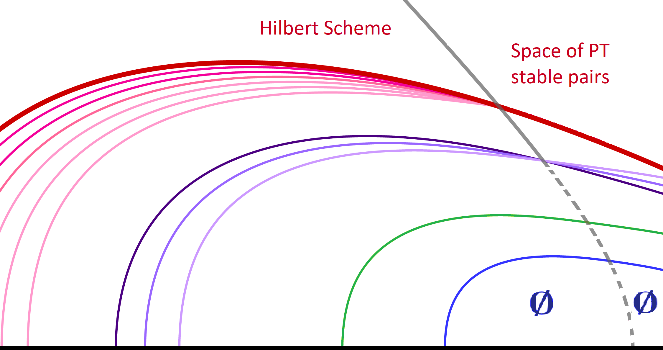
Figure 1. walls in Bridgeland stability space (in the $\alpha,\beta$ plane with $s=0.8$)

∎

4. Ext computation of the walls on the stable pairs side

So far, we have described all the possible walls in $\mathop{\mathrm{Stab}}\nolimits(\mathbb{P}^{3})$ close to the left branch of the hyperbola $\beta^{2}-\alpha^{2}=12$. To study the wall-crossing and describe the chambers (on the right side of the hyperbola) in section 5, we need to compute all the necessary $\mathrm{Ext}^{1}$-groups associated with the walls. When there is no confusion, we use the notation $A$ and $B$ for the subobject and the quotient of the defining short exact sequence of any wall, respectively.

First, we have the following lemma to compute the pull-backs:

Lemma 4.1.

For a plane $P$, a line $L$, a line $L^{\prime}\subset P$, a conic $C_{2}=L\cup L^{\prime}$, a 0-dimensional subscheme $Z$, and $\iota_{P}\colon P\hookrightarrow\mathbb{P}^{3}$ we have

$$\iota_{P}^{*}(\mathcal{I}_{L})=\begin{cases}\mathcal{I}_{L\cap P/P},&L\not\subset P\\ \mathcal{O}_{P}(-1)\oplus\mathcal{O}_{L}(-1),&L\subset P\par\\ \end{cases}$$

$$\iota_{P}^{*}(\mathcal{O}\xrightarrow{s}\mathcal{O}_{L}(1))=\begin{cases}\mathcal{I}_{L\cap P},&L\not\subset P,\\ &\text{zero locus of $s$ is not $L\cap P$}\\ \mathcal{O}_{P}\oplus\mathcal{O}_{L\cap P}[-1],&L\not\subset P,\\ &\text{zero locus of $s$ is $L\cap P$}\\ (\mathcal{O}_{P}\rightarrow\mathcal{O}_{L}(1))\oplus\mathcal{O}_{L},&L\subset P\par\\ \end{cases}$$

$$\iota_{P}^{*}(\mathcal{O}\xrightarrow{s}\mathcal{O}_{L}(2))=\begin{cases}\mathcal{I}_{L\cap P},&L\not\subset P,\\ &\text{zero locus of $s$ does not contain $L\cap P$}\\ \mathcal{O}_{P}\oplus\mathcal{O}_{L\cap P}[-1],&L\not\subset P,\\ &\text{zero locus of $s$ contains $L\cap P$}\\ (\mathcal{O}_{P}\rightarrow\mathcal{O}_{L}(2))\oplus\mathcal{O}_{L}(1),&L\subset P\par\\ \end{cases}$$

Proof.

The first two equations are proven in [23].

Now, let us compute $\iota_{P}^{*}(\mathcal{O}\rightarrow\mathcal{O}_{L}(1))$. First, assume that $L\not\subset P$, and the zero locus of $s$ is not $L\cap P$. Then we have $\iota_{P}^{*}(\mathcal{O}\rightarrow\mathcal{O}_{L}(1))=(\mathcal{O}_{P}\rightarrow\mathcal{O}_{L\cap P})=\mathcal{I}_{L\cap P}$. Secondly, assume that $L\not\subset P$, and the zero locus of $s$ is $L\cap P$. Then from the sequence $\mathcal{O}_{L}(1)[-1]\rightarrow(\mathcal{O}\rightarrow\mathcal{O}_{L}(1))\rightarrow\mathcal{O}$, we have $\iota_{P}^{*}(\mathcal{O}\rightarrow\mathcal{O}_{L}(1))=\mathcal{O}_{P}\oplus\mathcal{O}_{L\cap P}[-1]$.

Now, let us assume $L\subset P$. In this case, we have $\iota_{P}^{*}(\mathcal{O}\rightarrow\mathcal{O}_{L}(1))=\iota_{P}^{*}(\mathcal{O}\rightarrow\mathcal{I}_{L}(1)\rightarrow\mathcal{O}(1))=\mathcal{O}_{P}\rightarrow\iota_{P}^{*}(\mathcal{I}_{L}(1))\rightarrow\mathcal{O}_{P}(1)$. Hence from the first part we obtain $\mathcal{O}_{P}\rightarrow\mathcal{O}_{L}\oplus\mathcal{O}_{P}\rightarrow\mathcal{O}_{P}(1)=(\mathcal{O}_{P}\rightarrow\mathcal{O}_{L})\oplus\mathcal{O}_{L}(1)=(\mathcal{O}_{P}\rightarrow\mathcal{O}_{L}(1))\oplus\mathcal{O}_{L}$.

A similar argument implies the result for $\iota_{P}^{*}(\mathcal{O}\rightarrow\mathcal{O}_{L}(2))$.

∎

We have the following Lemmas on the $\mathrm{Ext}^{1}$’s:

Lemma 4.2.

For the wall $\langle\mathcal{I}_{C_{2}}(-1),\mathcal{O}_{P}(-4)\rangle$, we have:

$$\mathrm{Ext}^{1}(\mathcal{I}_{C_{2}}(-1),\mathcal{I}_{C_{2}}(-1))=\mathbb{C}^{8}, \mathrm{Ext}^{1}(\mathcal{O}_{P}(-4),\mathcal{O}_{P}(-4))=\mathbb{C}^{3},$$

$$\mathrm{Ext}^{1}(\mathcal{O}_{P}(-4),\mathcal{I}_{C_{2}}(-1))=\mathbb{C}^{13}, \mathrm{Ext}^{1}(\mathcal{I}_{C_{2}}(-1),\mathcal{O}_{P}(-4))=\mathbb{C}.$$

Proof.

This is just a straightforward computation. ∎

Lemma 4.3 ([23, Lemma 4.3]).

For the wall $\langle\mathcal{I}_{L}(-1),\iota_{P_{*}}(\mathcal{I}_{Z_{2}})^{\vee}(-5)\rangle$, we have:

$$\mathrm{Ext}^{1}(\mathcal{I}_{L}(-1),\mathcal{I}_{L}(-1))=\mathbb{C}^{4},\quad\mathrm{Ext}^{1}(\iota_{P_{*}}(\mathcal{I}_{Z_{2}})^{\vee}(-5),\iota_{P_{*}}(\mathcal{I}_{Z_{2}})^{\vee}(-5))=\mathbb{C}^{7},$$

$$\mathrm{Ext}^{1}(\iota_{P_{*}}(\mathcal{I}_{Z_{2}})^{\vee}(-5),\mathcal{I}_{L}(-1))=\mathbb{C}^{18},$$

$$\mathrm{Ext}^{1}(\mathcal{I}_{L}(-1),\iota_{P_{*}}(\mathcal{I}_{Z_{2}})^{\vee}(-5))=\begin{cases}0,&\langle Z_{2}\rangle\cap L=\emptyset\\ \mathbb{C},&\text{ $\langle Z_{2}\rangle\cap L\neq\emptyset$ but $\langle Z_{2}\rangle\neq L$}\\ \mathbb{C}^{2},&\langle Z_{2}\rangle=L\par\par\par\end{cases}$$

where $\langle Z_{2}\rangle$ is the line spanned by $Z_{2}$.

In the statement of the following Lemma, all tensor products are in $\mathrm{D}^{b}(P)$:

Lemma 4.4.

Let $p\neq q$ be two different points in a plane $P$, such that $p\subset l$, and $p\not\subset l^{\prime}$, for lines $l,l^{\prime}$ in $P$. Then $\mathcal{I}_{p}\otimes\mathcal{I}_{p}$ fits into the short exact sequence $\mathcal{O}_{p}\hookrightarrow\mathcal{I}_{p}\otimes\mathcal{I}_{p}\twoheadrightarrow{}\mathcal{I}^{2}_{p}$. Also, $\mathcal{I}_{p\cup q}\otimes\mathcal{I}_{p}$ fits into the short exact sequence $\mathcal{O}_{p}\hookrightarrow\mathcal{I}_{p\cup q}\otimes\mathcal{I}_{p}\twoheadrightarrow{}\mathcal{I}_{p^{2}\cup q}$. Furthermore, we have

$$\mathcal{I}_{p}\otimes\mathcal{O}_{p}=\mathcal{O}_{p}[1]\oplus\mathcal{O}_{p}^{\oplus 2},\quad\mathcal{I}_{p}\otimes\mathcal{O}_{q}=\mathcal{O}_{q},\quad\mathcal{I}_{p}\otimes\mathcal{I}_{q}=\mathcal{I}_{p\cup q},$$

$$\quad\mathcal{I}_{p}\otimes\mathcal{O}_{l}=\mathcal{O}_{l}(-1)\oplus\mathcal{O}_{p},\quad\mathcal{I}_{p}\otimes\mathcal{O}_{l^{\prime}}=\mathcal{O}_{l^{\prime}}.$$

Proof.

All the cases either proved in [23, Lemma 4.2] or exactly a similar argument there implies the result.

∎

Lemma 4.5.

For the wall $\langle\mathcal{O}(-1)\rightarrow\mathcal{O}_{L},\iota_{P_{*}}\mathcal{I}_{Z_{1}}^{\vee}(-5)\rangle$, we have

$$\mathrm{Ext}^{1}((\mathcal{O}(-1)\rightarrow\mathcal{O}_{L}),(\mathcal{O}(-1)\rightarrow\mathcal{O}_{L}))=\mathbb{C}^{5},\quad\mathrm{Ext}^{1}(\iota_{P_{*}}\mathcal{I}_{Z_{1}}^{\vee}(-5),\iota_{P_{*}}\mathcal{I}_{Z_{1}}^{\vee}(-5))=\mathbb{C}^{5},$$

$$\mathrm{Ext}^{1}(\iota_{P_{*}}\mathcal{I}_{Z_{1}}^{\vee}(-5),\mathcal{O}(-1)\xrightarrow{s}\mathcal{O}_{L})=\begin{cases}\mathbb{C}^{21},&\text{the zero locus of $s$ is at $Z_{1}$,}\\ \mathbb{C}^{20},&\text{the zero locus of $s$ is in $P$ but $\neq Z_{1}$},\\ \mathbb{C}^{19},&\text{the zero locus of $s$ is not in $P$}\end{cases}$$

$$\mathrm{Ext}^{1}(\mathcal{O}(-1)\xrightarrow{s}\mathcal{O}_{L},\iota_{P_{*}}\mathcal{I}_{Z_{1}}^{\vee}(-5))=\begin{cases}\mathbb{C}^{2},&\text{the zero locus of $s$ is at $Z_{1}$},\\ \mathbb{C},&\text{ the zero locus of $s$ is in $P$ but $\neq Z_{1}$},\\ 0,&\text{the zero locus of $s$ is not in $P$}\end{cases}$$

Proof.

We notice that $\mathrm{Ext}^{1}(\mathcal{O}(-1)\rightarrow\mathcal{O}_{L},\mathcal{O}(-1)\rightarrow\mathcal{O}_{L})$ generically parametrizes a line in $\mathbb{P}^{3}$ (given by $\mathbb{G}r(2,4)$) together with a choice of one point on the line. Thus we have $\mathrm{Ext}^{1}(\mathcal{O}(-1)\rightarrow\mathcal{O}_{L},\mathcal{O}(-1)\rightarrow\mathcal{O}_{L})=\mathbb{C}^{5}$. Also, $\mathrm{Ext}^{1}(\iota_{P_{*}}\mathcal{I}_{Z_{1}}^{\vee}(-5),\iota_{P_{*}}\mathcal{I}_{Z_{1}}^{\vee}(-5))$ is the parameter space of one point in a plane, which gives the flag variety $\mathfrak{Fl}_{1}$. Therefore we have $\mathrm{Ext}^{1}(B,B)=\mathbb{C}^{5}$.

Let $q$ be the zero locus of $s$. Now we compute $\mathrm{Ext}^{1}(B,A)$ as follows:

$$\mathrm{Ext}^{1}(\iota_{P_{*}}\mathcal{I}_{Z_{1}}^{\vee}(-5),\mathcal{O}(-1)\rightarrow\mathcal{O}_{L})=\mathrm{H}^{0}\bigl{(}\iota_{P}^{*}(\mathcal{O}\rightarrow\mathcal{O}_{L}(1))\otimes\mathcal{I}_{Z_{1}}(5)\bigr{)}.$$

First, assume that $L\not\subset P$:

There are two cases:

• (I) Zero locus of $s$ is not at $L\cap P$: Using Lemmas 4.1 and 4.4 we have:

  (i) if $L\cap P=Z_{1}$, then we have $\mathrm{H}^{0}(\iota_{P}^{*}(\mathcal{O}\rightarrow\mathcal{O}_{L}(1))\otimes\mathcal{I}_{Z_{1}}(5))=\mathrm{H}^{0}(\mathcal{I}_{L\cap P}\otimes\mathcal{I}_{Z_{1}}(5))=\mathrm{H}^{0}(\mathcal{I}_{Z_{1}}\otimes\mathcal{I}_{Z_{1}}(5))=\mathrm{H}^{0}(\mathcal{O}_{Z_{1}})\oplus\mathrm{H}^{0}(\mathcal{I}_{Z_{1}}^{2}(5))=\mathbb{C}^{19}$.

  (ii) if $L\cap P\neq Z_{1}$, then we have $\mathrm{H}^{0}(\iota_{P}^{*}(\mathcal{O}\rightarrow\mathcal{O}_{L}(1))\otimes\mathcal{I}_{Z_{1}}(5)))=\mathrm{H}^{0}(\mathcal{I}_{L\cap P}\otimes\mathcal{I}_{Z_{1}}(5))=\mathrm{H}^{0}(\mathcal{I}_{(L\cap P)\cup Z_{1}}(5))=\mathbb{C}^{19}$.

• (II) Zero locus of $s$ is $L\cap P$: By Lemma 4.1, we have $\mathrm{H}^{0}(\iota_{P}^{*}(\mathcal{O}\rightarrow\mathcal{O}_{L}(1))\otimes\mathcal{I}_{Z_{1}}(5))=\mathrm{H}^{0}((\mathcal{O}_{P}\oplus\mathcal{O}_{L\cap P}[-1])\otimes\mathcal{I}_{Z_{1}}(5))=\mathrm{H}^{0}(\mathcal{O}_{P}\otimes\mathcal{I}_{Z_{1}}(5))\oplus\mathrm{H}^{-1}(\mathcal{O}_{L\cap P}\otimes\mathcal{I}_{Z_{1}}(5))=\mathrm{H}^{0}(\mathcal{I}_{Z_{1}}(5))\oplus\mathrm{H}^{-1}(\mathcal{O}_{L\cap P}\otimes\mathcal{I}_{Z_{1}}(5))=\mathbb{C}^{20}\oplus\mathrm{H}^{-1}(\mathcal{O}_{L\cap P}\otimes\mathcal{I}_{Z_{1}}(5))$. Now there are two subcases:

  (i) if $Z_{1}\neq P\cap L$, by Lemma 4.4 we have $\mathrm{Ext}^{1}(B,A)=\mathbb{C}^{20}\oplus\mathrm{H}^{-1}(\mathcal{O}_{L\cap P}\otimes\mathcal{I}_{Z_{1}}(5))=\mathbb{C}^{20}\oplus\mathrm{H}^{-1}(\mathcal{O}_{L\cap P})=\mathbb{C}^{20}\oplus 0=\mathbb{C}^{20}$.

  (ii) if $Z_{1}=P\cap L$, by Lemma 4.4 we have $\mathcal{O}_{L\cap P}\otimes\mathcal{I}_{Z_{1}}(1)=\mathcal{O}_{Z_{1}}[1]\oplus\mathcal{O}^{\oplus 2}_{Z_{1}}$, and therefore $\mathrm{Ext}^{1}(B,A)=\mathrm{H}^{0}(\mathcal{I}_{Z_{1}}(5))\oplus\mathrm{H}^{0}(\mathcal{O}_{Z_{1}})=\mathbb{C}^{20}\oplus\mathbb{C}^{1}=\mathbb{C}^{21}.$

Second, assume that $L\subset P$:

In this case we have $\iota_{P}^{*}(\mathcal{O}\rightarrow\mathcal{O}_{L}(1))=(\mathcal{O}_{P}\rightarrow\mathcal{O}_{L}(1))\oplus\mathcal{O}_{L}$. Therefore we have

$$\mathop{\mathrm{Ext}}\nolimits^{1}(B,A)=\mathrm{H}^{0}(\iota_{P}^{*}(\mathcal{O}\rightarrow\mathcal{O}_{L}(1))\otimes\mathcal{I}_{Z_{1}}(5))=\mathrm{H}^{0}((\mathcal{O}_{P}(5)\rightarrow\mathcal{O}_{L}(6))\otimes\mathcal{I}_{Z_{1}})\oplus\mathrm{H}^{0}(\mathcal{O}_{L}\otimes\mathcal{I}_{Z_{1}}(5))$$

$$=\mathrm{H}^{0}(\mathcal{I}_{Z_{1}}(5)\rightarrow\mathcal{O}_{L}\otimes\mathcal{I}_{Z_{1}}(6))\oplus\mathrm{H}^{0}(\mathcal{O}_{L}\otimes\mathcal{I}_{Z_{1}}(5)).$$

But using 4.4 we have

$$\mathrm{H}^{0}(\mathcal{O}_{L}\otimes\mathcal{I}_{Z_{1}}(5))=\begin{cases}\mathrm{H}^{0}(\mathcal{O}_{L}(5))\cong\mathbb{C}^{6},&Z_{1}\not\subset L,\\ \mathrm{H}^{0}(\mathcal{O}_{L}(4)\oplus\mathcal{O}_{Z_{1}})=\mathbb{C}^{5}\oplus\mathbb{C}\cong\mathbb{C}^{6},&Z_{1}\subset L.\par\par\end{cases}$$

On the other hand, to compute $\mathrm{H}^{0}(\mathcal{I}_{Z_{1}}(5)\xrightarrow{s}\mathcal{O}_{L}\otimes\mathcal{I}_{Z_{1}}(6))=\mathrm{H}^{0}(\ker(s))$, we notice that $s$ factors as follows: $\mathcal{I}_{Z_{1}}(5)\xrightarrow{s_{1}}\mathcal{O}_{L}\otimes\mathcal{I}_{Z_{1}}(5)\xrightarrow{s_{2}}\mathcal{O}_{L}\otimes\mathcal{I}_{Z_{1}}(6).$ Note that $\ker(s_{1})=\mathcal{I}_{Z_{1}}(4)$. Now there are three cases:

• (1) If $Z_{1}\not\subset L$, then by Lemma 4.4 we have $s_{2}\colon\mathcal{O}_{L}(5)\to\mathcal{O}_{L}(6)$, which is injective.

• (2) If $Z_{1}\subset L$, but $Z_{1}\neq\text{zero locus of $s$}$, then by Lemma 4.4 we have $s_{2}\colon\mathcal{O}_{L}(4)\oplus\mathcal{O}_{Z_{1}}\to\mathcal{O}_{L}(5)\oplus\mathcal{O}_{Z_{1}}$, which is injective.

• (3) If $Z_{1}=\text{zero locus of $s\subset L$}$, then $s_{2}|_{\mathcal{O}_{Z_{1}}}=0$.

For cases (1) and (2), where $s_{2}$ is injective, we have

$$\mathrm{H}^{0}(\ker(s))=\mathrm{H}^{0}(\ker(s_{1}))=\mathrm{H}^{0}(\mathcal{I}_{Z_{1}}(4))=\mathbb{C}^{14}.$$

For case (3), similarly using Lemma 4.4, we have

$$\mathrm{H}^{0}(\ker(s))=\mathrm{H}^{0}(\ker(\mathcal{I}_{Z_{1}}(5)\to\mathcal{O}_{L}(4)))=\mathrm{H}^{0}(\mathcal{O}_{P}(4))=\mathbb{C}^{15}.$$

Thus $\mathop{\mathrm{Ext}}\nolimits^{1}(B,A)$ is

$$\mathrm{H}^{0}(\mathcal{I}_{Z_{1}}(5)\rightarrow\mathcal{O}_{L}\otimes\mathcal{I}_{Z_{1}}(6))\oplus\mathrm{H}^{0}(\mathcal{O}_{L}\otimes\mathcal{I}_{Z_{1}}(5))=\begin{cases}\mathbb{C}^{14}\oplus\mathbb{C}^{6}=\mathbb{C}^{20},&Z_{1}\neq q,\\ \mathbb{C}^{15}\oplus\mathbb{C}^{6}=\mathbb{C}^{21},&Z_{1}=q\subset L.\par\par\end{cases}$$

For the last part, using Serre duality we have

$$\mathrm{Ext}^{1}(A,B)=\mathrm{Ext}^{1}(\mathcal{O}(-1)\rightarrow\mathcal{O}_{L},\iota_{P_{*}}\mathcal{I}_{Z_{1}}^{\vee}(-5))=\mathrm{Ext}^{1}((\iota_{P}^{*}(\mathcal{O}(-1)\rightarrow\mathcal{O}_{L}),\mathcal{I}_{Z^{\prime}_{1}}^{\vee}(-5))$$

$$=\mathrm{Ext}^{1}(\mathcal{I}_{Z^{\prime}_{1}}^{\vee}(-5),(\iota_{P}^{*}(\mathcal{O}(-1)\rightarrow\mathcal{O}_{L})\otimes\mathcal{O}(-3))^{\vee}=\mathrm{H}^{1}((\iota_{P}^{*}(\mathcal{O}(-1)\rightarrow\mathcal{O}_{L})\otimes\mathcal{I}_{Z_{1}}(2))^{\vee}.$$

There are three cases:

(1) $L\not\subset P$ and $L\cap P$ is the zero locus of $s$:

: From Lemmas 4.1 and 4.4, we have

$$\mathrm{Ext}^{1}(A,B)=\mathrm{H}^{1}((\iota_{P}^{*}(\mathcal{O}\rightarrow\mathcal{O}_{L}(1))\otimes\mathcal{I}_{Z_{1}}(1))^{\vee}=\mathrm{H}^{1}(\mathcal{I}_{Z_{1}}(1))^{\vee}\oplus\mathrm{H}^{0}(\mathcal{O}_{L\cap P}\otimes\mathcal{I}_{Z_{1}}(1))^{\vee}$$

$$=0\oplus\mathrm{H}^{0}(\mathcal{O}_{L\cap P}\otimes\mathcal{I}_{Z_{1}}(1))^{\vee}=\begin{cases}\mathrm{H}^{0}(\mathcal{O}_{P\cap L})^{\vee}=\mathbb{C},&L\cap P\neq Z_{1}\\ \mathrm{H}^{0}(\mathcal{O}_{L\cap P}[1]\oplus\mathcal{O}_{L\cap P}^{\oplus 2})^{\vee}=0\oplus\mathbb{C}^{2}=\mathbb{C}^{2},&L\cap P=Z_{1}\\ \end{cases}$$

(2) $L\not\subset P$, and $L\cap P$ is not the zero section of $s$:

: From Lemmas 4.1 and 4.4, we have

$$\mathrm{Ext}^{1}(A,B)=\mathrm{H}^{1}(\mathcal{I}_{L\cap P}\otimes\mathcal{I}_{Z_{1}}(1))^{\vee}$$

$$=\begin{cases}\mathrm{H}^{1}(\mathcal{I}_{(P\cap L)\cup Z_{1}}(1))^{\vee}=0,&L\cap P\neq Z_{1}\\ \mathrm{H}^{1}(\mathcal{O}_{L\cap P})^{\vee}\oplus\mathrm{H}^{1}(\mathcal{I}_{L\cap P}^{2}(1))^{\vee}=0\oplus 0=0,&L\cap P=Z_{1}\\ \end{cases}$$

(3) $L\subset P$:

: Again using Lemmas 4.1, we have

$$\mathrm{Ext}^{1}(A,B)=\mathrm{H}^{1}((\mathcal{O}_{P}\xrightarrow{s}\mathcal{O}_{L}(1))\otimes\mathcal{I}_{Z_{1}}(1))^{\vee}\oplus\mathrm{H}^{1}(\mathcal{O}_{L}\otimes\mathcal{I}_{Z_{1}}(1))^{\vee}$$

$$=\mathrm{H}^{1}((\mathcal{O}_{P}\xrightarrow{s}\mathcal{O}_{L}(1))\otimes\mathcal{I}_{Z_{1}}(1))^{\vee}\oplus 0.$$

Exactly the same argument as above (just twisting everything by $-4$) implies

$$\mathrm{H}^{0}(\mathcal{I}_{Z_{1}}(1)\rightarrow\mathcal{O}_{L}\otimes\mathcal{I}_{Z_{1}}(2))=\begin{cases}0,&Z_{1}\neq\text{zero locus of $s$},\\ \mathbb{C},&Z_{1}=\text{zero locus of $s\subset L$}.\par\par\end{cases}$$

Now, taking the cohomology long exact sequence of $\mathcal{O}_{L}\otimes\mathcal{I}_{Z_{1}}(2)[-1]\rightarrow(\mathcal{O}_{P}\rightarrow\mathcal{O}_{L}(1))\otimes\mathcal{I}_{Z_{1}}(1)\rightarrow\mathcal{O}_{P}\otimes\mathcal{I}_{Z_{1}}(1)$ and noticing that $\mathrm{H}^{0}(\mathcal{O}_{P}\otimes\mathcal{I}_{Z_{1}}(1))=\mathrm{H}^{0}(\mathcal{I}_{Z_{1}}(1))=\mathbb{C}^{2},$ and (by Lemma 4.4)

$$\mathrm{H}^{0}(\mathcal{O}_{L}\otimes\mathcal{I}_{Z_{1}}(2))=\begin{cases}\mathrm{H}^{0}(\mathcal{O}_{L}(2))\cong\mathbb{C}^{3},&Z_{1}\not\subset L,\\ \mathrm{H}^{0}(\mathcal{O}_{L}(1)\oplus\mathcal{O}_{Z_{1}})=\mathbb{C}^{2}\oplus\mathbb{C}\cong\mathbb{C}^{3},&Z_{1}\subset L,\par\par\end{cases}$$

we have

Therefore, in this case we have

$$\mathop{\mathrm{Ext}}\nolimits^{1}(A,B)=\mathrm{H}^{1}(\mathcal{I}_{Z_{1}}(1)\rightarrow\mathcal{O}_{L}\otimes\mathcal{I}_{Z_{1}}(2))^{\vee}=\begin{cases}\mathbb{C},&Z_{1}\neq\text{zero locus of $s$},\\ \mathbb{C}^{2},&Z_{1}=\text{zero locus of $s\subset L$}.\par\par\end{cases}$$

∎

Lemma 4.6.

For the wall $\langle\mathcal{O}(-1)\rightarrow\mathcal{O}_{L}(1),\mathcal{O}_{P}(-5)\rangle$, we have:

$$\mathrm{Ext}^{1}(\mathcal{O}(-1)\rightarrow\mathcal{O}_{L}(1),\mathcal{O}(-1)\rightarrow\mathcal{O}_{L}(1))=\mathbb{C}^{6},\quad\mathrm{Ext}^{1}(\mathcal{O}_{P}(-5),\mathcal{O}_{P}(-5))=\mathbb{C}^{3},$$

$$\mathrm{Ext}^{1}(\mathcal{O}_{P}(-5),\mathcal{O}(-1)\xrightarrow{s}\mathcal{O}_{L}(1))=\begin{cases}\mathbb{C}^{22},&\text{ $L\subset P$}\\ \mathbb{C}^{21},&\text{$L\not\subset P$, and the zero locus of $s\supset L\cap P$},\\ \mathbb{C}^{20},&\text{$L\not\subset P$, and the zero locus of $s\not\supset L\cap P$}\par\par\par\par\end{cases}$$

$$\mathrm{Ext}^{1}(\mathcal{O}(-1)\xrightarrow{s}\mathcal{O}_{L}(1),\mathcal{O}_{P}(-5))=\begin{cases}\mathbb{C}^{2},&L\subset P,\par\\ \mathbb{C},&\text{$L\not\subset P$ and the zero locus of $s\supset L\cap P$}\\ 0,&\text{$L\not\subset P$, and the zero locus of $s\not\supset L\cap P$}\end{cases}$$

Proof.

We notice that $\mathrm{Ext}^{1}((\mathcal{O}\rightarrow\mathcal{O}_{L}(2))\otimes\mathcal{O}(-1),(\mathcal{O}\rightarrow\mathcal{O}_{L}(2))\otimes\mathcal{O}(-1))$ generically parametrizes a line in $\mathbb{P}^{3}$ (given by $\mathbb{G}r(2,4)$) together with a choice of two points on the line. Thus we have $\mathrm{Ext}^{1}(\mathcal{O}(-1)\rightarrow\mathcal{O}_{L}(1),\mathcal{O}(-1)\rightarrow\mathcal{O}_{L}(1))=\mathbb{C}^{6}$. Also, $\mathrm{Ext}^{1}(\iota_{P_{*}}(\mathcal{O}_{P})(-5),\iota_{P_{*}}(\mathcal{O}_{P})(-5))$ is the parameter space of a plane in $\mathbb{P}^{3}$ which is given by $(\mathbb{P}^{3})^{*}$, and thus $\mathrm{Ext}^{1}(B,B)=\mathbb{C}^{3}$.

Let $q\cup q^{\prime}$ be the zero locus of $s$. Now we compute $\mathrm{Ext}^{1}(B,A)$ as follows:

$$\mathrm{Ext}^{1}(B,A)=\mathrm{Ext}^{1}(\iota_{P_{*}}(\mathcal{O}_{P})(-5),\mathcal{O}(-1)\rightarrow\mathcal{O}_{L}(1))=\mathrm{Ext}^{1}(\mathcal{O}_{P}(-5),\iota_{P}^{!}(\mathcal{O}(-1)\rightarrow\mathcal{O}_{L}(1)))$$

$$=\mathrm{Hom}(\mathcal{O}_{P}(-5),\iota_{P}^{*}(\mathcal{O}\rightarrow\mathcal{O}_{L}(2)))=\mathrm{H}^{0}(\iota_{P}^{*}(\mathcal{O}\rightarrow\mathcal{O}_{L}(2))\otimes\mathcal{O}(5)).$$

First, assume that $L\not\subset P$:

By Lemma 4.1 we have:

$$\mathrm{Ext}^{1}(B,A)=\begin{cases}\mathrm{H}^{0}((\mathcal{O}_{P}(5)\oplus\mathcal{O}_{L\cap P}[-1]))=\mathbb{C}^{21}\oplus 0,&q\cup q^{\prime}\supset L\cap P,\\ \mathrm{H}^{0}(\mathcal{I}_{L\cap P}(5))=\mathbb{C}^{20},&q\cup q^{\prime}\not\supset L\cap P.\end{cases}$$

Second, assume that $L\subset P$:

Using Lemma 4.1, we have $\mathrm{H}^{0}(\iota_{P}^{*}(\mathcal{O}\rightarrow\mathcal{O}_{L}(2))\otimes\mathcal{O}(5))=\mathrm{H}^{0}((\mathcal{O}_{P}\rightarrow\mathcal{O}_{L}(2))\otimes\mathcal{O}(5))\oplus\mathrm{H}^{0}(\mathcal{O}_{L}(1)\otimes\mathcal{O}(5))=\mathrm{H}^{0}((\mathcal{O}_{P}(5)\rightarrow\mathcal{O}_{L}(7)))\oplus\mathrm{H}^{0}(\mathcal{O}_{L}(6))$.

We have $\mathrm{H}^{0}((\mathcal{O}_{P}(5)\xrightarrow{s}\mathcal{O}_{L}(7)))=\mathrm{H}^{0}(\ker(s))=\mathrm{H}^{0}(\mathcal{I}_{L}(5))=\mathbb{C}^{15}$. Also, we have $\mathrm{H}^{0}(\mathcal{O}_{L}(6))=\mathbb{C}^{7}$. Therefore, $\mathrm{H}^{0}(\iota_{P}^{*}(\mathcal{O}\rightarrow\mathcal{O}_{L}(1))\otimes\mathcal{I}_{Z^{\prime}_{1}}(5))=\mathbb{C}^{15}\oplus\mathbb{C}^{7}=\mathbb{C}^{22}$.

Finally, for $\mathrm{Ext}^{1}(A,B)$ using Serre duality, we have

$$\mathrm{Ext}^{1}((\mathcal{O}(-1)\rightarrow\mathcal{O}_{L}(1)),\mathcal{O}_{P}(-5))=\mathrm{H}^{1}(\iota_{P}^{*}(\mathcal{O}\rightarrow\mathcal{O}_{L}(2))\otimes\mathcal{O}(1))^{\vee}.$$

1) If $L\subset P$:

:

$$\mathrm{Ext}^{1}(A,B)=\mathrm{H}^{1}(\mathcal{O}_{P}(1)\xrightarrow{s}\mathcal{O}_{L}(3))^{\vee}\oplus\mathrm{H}^{1}(\mathcal{O}_{L}(2))^{\vee}=\mathrm{H}^{1}(\mathcal{O}_{P}(1)\xrightarrow{s}\mathcal{O}_{L}(3))^{\vee}\oplus 0.$$

We have $\mathrm{H}^{0}(\mathcal{O}_{P}(1)\xrightarrow{s}\mathcal{O}_{L}(3))=\mathrm{H}^{0}(\ker(s))=\mathrm{H}^{0}(\mathcal{I}_{L}(1))=\mathbb{C}$. Now, taking the long exact sequence of $\mathcal{O}_{L}(3)[-1]\rightarrow(\mathcal{O}_{P}(1)\xrightarrow{s}\mathcal{O}_{L}(3))\rightarrow\mathcal{O}_{P}(1)$, gives

which implies $\mathrm{H}^{1}(\mathcal{O}_{P}(1)\rightarrow\mathcal{O}_{L}(3))=\mathbb{C}^{2}$.

2) If $L\not\subset P$:

, using Lemma 4.1, we have

$$\mathrm{Ext}^{1}(A,B)=\begin{cases}\mathrm{H}^{1}(\mathcal{O}_{P}(1))^{\vee}\oplus\mathrm{H}^{0}(\mathcal{O}_{L\cap P})^{\vee}=0\oplus\mathbb{C},&q\cup q^{\prime}\supset L\cap P,\\ \mathrm{H}^{1}(\mathcal{I}_{L\cap P}(1))^{\vee}=0,&q\cup q^{\prime}\not\supset L\cap P.\par\par\par\par\end{cases}$$

∎

Lemma 4.7.

For the wall $\langle\mathcal{O}(-1),\iota_{P_{*}}\mathcal{I}_{Z_{6}}^{\vee}(-6)\rangle$, we have:

$$\mathrm{Ext}^{1}(\mathcal{O}(-1),\mathcal{O}(-1))=0,\quad\mathrm{Ext}^{1}(\iota_{P_{*}}\mathcal{I}_{Z_{6}}^{\vee}(-6),\iota_{P_{*}}\mathcal{I}_{Z_{6}}^{\vee}(-6))=\mathbb{C}^{15},$$

$$\mathrm{Ext}^{1}(\iota_{P_{*}}\mathcal{I}_{Z_{6}}^{\vee}(-6),\mathcal{O}(-1))=\mathbb{C}^{22},$$

$$\mathrm{Ext}^{1}(\mathcal{O}(-1),\iota_{P_{*}}\mathcal{I}_{Z_{6}}^{\vee}(-6))=\begin{cases}\mathbb{C}^{3},&\text{6 points on a line}\\ \mathbb{C}^{2},&\text{5 points on a line}\\ \mathbb{C},&\text{6 points on a conic}\\ 0,&\text{generic points}\\ \end{cases}$$

Proof.

The first statement is obvious. We notice that $\mathrm{Ext}^{1}(\iota_{P_{*}}\mathcal{I}_{Z_{6}}^{\vee}(-6),\iota_{P_{*}}\mathcal{I}_{Z_{6}}^{\vee}(-6))$ is a parameter space of six points in a plane which is of dimension 15 as claimed.

Now we compute $\mathrm{Ext}^{1}(B,A)$:

$$\mathrm{Ext}^{1}(\iota_{P_{*}}\mathcal{I}_{Z_{6}}^{\vee}(-6),\mathcal{O}(-1))=\mathrm{Hom}(\mathcal{I}_{Z^{\prime}_{6}}^{\vee}(-6),\iota_{P}^{*}(\mathcal{O}))=\mathrm{H}^{0}(\mathcal{I}_{Z^{\prime}_{6}}(6))=\mathbb{C}^{22}.$$

For the last part, using Serre duality we have

$$\mathrm{Ext}^{1}(\mathcal{O}(-1),\iota_{P_{*}}\mathcal{I}_{Z_{6}}^{\vee}(-6))=\mathrm{Ext}^{1}(\iota_{P}^{*}\mathcal{O}(-1),\mathcal{I}_{Z^{\prime}_{6}}^{\vee}(-6))=\mathrm{H}^{1}(\mathcal{O}_{P}\otimes\mathcal{I}_{Z^{\prime}_{6}}(2))^{\vee}=\mathrm{H}^{1}(\mathcal{I}_{Z^{\prime}_{6}}(2))^{\vee}$$

$$=\begin{cases}\mathbb{C}^{3},&\text{6 points on a line}\\ \mathbb{C}^{2},&\text{5 points on a line}\\ \mathbb{C},&\text{6 points on a conic}\\ 0,&\text{generic points}\\ \end{cases}$$

as $\mathop{\mathrm{dim}}\nolimits\mathrm{H}^{1}(\mathcal{I}_{Z^{\prime}_{6}}(2))^{\vee}=\mathop{\mathrm{dim}}\nolimits\mathrm{H}^{0}(\mathcal{I}_{Z^{\prime}_{6}}(2))^{\vee}$ by taking a long exact sequence of $\mathcal{I}_{Z^{\prime}_{6}}(2)\to\mathcal{O}_{P}(2)\to\mathcal{O}_{Z^{\prime}_{6}}$.

∎

5. Chambers

In this section, we describe the corresponding moduli spaces to the chambers close to the hyperbola from the right.

First, we need the following Lemma which gives a condition under which we can realize what components can survive all the way to the large volume limit:

Lemma 5.1.

Suppose that $\mathcal{H}^{0}$ of a general object in an irreducible component created by a wall is an ideal sheaf. Then this irreducible component survives all the way up to the moduli space of stable pairs.

Proof.

As stability is an open condition, we only need to show this for one object which is created after each wall. If an object $E$ is destabilized by a subobject $E^{\prime}$, there is an injection $E^{\prime}\hookrightarrow E$ in $\mathrm{Coh}^{\alpha,\beta}(\mathbb{P}^{3})$ which induces an injection $\mathcal{H}^{0}(E^{\prime})\hookrightarrow\mathcal{H}^{0}(E)$. By assumption, $\mathcal{H}^{0}$ of a general object created by the wall is an ideal sheaf $\mathcal{I}$. On the other hand, $\mathcal{H}^{0}$ of the destabilizing subobjects are all of the form $\mathcal{O}_{P}(-i)$, by Theorem 3.12. But we have $\mathop{\mathrm{Hom}}\nolimits(\mathcal{O}_{P}(-i),\mathcal{I})=0$, therefore the induced map on $\mathcal{H}^{0}$ is not injective, which is a contradiction. This implies the result. ∎

We also need the following Lemma:

Lemma 5.2.

Suppose that $E$ is a sheaf with $c_{0}(E)=1$ and $c_{1}(E)=0$, such that it fits into $\mathcal{I}_{D}(-1)\hookrightarrow E\twoheadrightarrow\mathcal{O}_{P}(-k)$, for $\mathcal{I}_{D}$ an ideal sheaf of a subscheme $D$ transverse to the plane $P$, and $k$ a positive integer. Then $E$ is an ideal sheaf of a curve.

Proof.

First, we observe that $\iota_{P}^{*}(\mathcal{I}_{D})=\mathcal{I}_{D\cap P/P}$. In order to show that $E$ is an ideal sheaf of a curve, we need to show that it is torsion-free. We know that any subsheaf of $\mathcal{O}_{P}(-k)$ contains a subsheaf of the form $\mathcal{O}_{P}(-i)$ for some $k<i$. It is enough to show that such $\mathcal{O}_{P}(-i)$ does not lift to a subsheaf of $E$. Using the identification $\mathrm{Ext}^{1}(\mathcal{O}_{P}(-i),\mathcal{I}_{D}(-1))=\mathrm{Ext}^{1}(\mathcal{O}_{P}(-i),\iota^{*}_{P}\mathcal{I}_{D}(-1)(1)[-1])=\mathrm{H}^{0}(\mathcal{I}_{D\cap P/P}(i))$, one can see that $\mathrm{Ext}^{1}(\mathcal{O}_{P}(-k),\mathcal{I}_{D}(-1))\hookrightarrow\mathrm{Ext}^{1}(\mathcal{O}_{P}(-i),\mathcal{I}_{D}(-1))$ is injective. Hence $\mathcal{O}_{P}(-i)$ does not lift to a subsheaf of $E$. ∎

Proposition 5.3 ([23, Proposition 3.14]).

The moduli space for the first chamber below the first wall, which is given by all the extensions of two objects $\mathcal{O}(-2),\mathcal{O}_{Q}(-3)$, is empty.

Let $\mathcal{N}_{1}$ be the first non-empty moduli space for the next chamber, which appears after crossing the smallest wall $\langle\mathcal{O}(-2),\mathcal{O}_{Q}(-3)\rangle$. In the following Proposition from [23], we see that this moduli space gives a compactification of objects corresponding to $(2,3)$-complete intersection curves in $\mathbb{P}^{3}$:

Proposition 5.4 ([23, Proposition 3.15]).

The moduli space $\mathcal{N}_{1}$ is a $\mathbb{P}^{15}$-bundle over $\mathbb{P}^{9}$. More precisely, the complement of (2,3)-complete intersections in $\mathcal{N}_{1}$ are parametrized by the pairs $(Q,C)$ where $Q=P\cup P^{\prime}$ is a union of two planes and $C$ is a conic in one of the two planes. The associated objects are non-torsion free sheaves $E$ given by $\mathcal{O}_{P}(-4)\hookrightarrow E\twoheadrightarrow\mathcal{I}_{C_{2}}(-1),$ for a conic $C_{2}$. The generic element is given by an ideal sheaf of (2,3)-complete intersection curves.

Proof.

The only remaining part which was not covered in [23], is the description of the generic element as an ideal sheaf: this is easily obtained by noticing that $\mathcal{H}^{1}(\mathcal{O}(-2))=0$, and then taking the long exact sequence of the defining sequence $\mathcal{O}(-2)\hookrightarrow E\twoheadrightarrow\mathcal{O}_{Q}(-3)$ and applying Lemma 5.2 to $D=P^{\prime}$. ∎

Before describing the next chambers, we need the following Lemmas:

Lemma 5.5 ([8, Lemma 4.4]).

Let $F\hookrightarrow E\twoheadrightarrow G$ be an exact sequence at a wall in Bridgeland stability with $E$ semistable to one side of the wall and $F,G$ distinct stable objects of the same (Bridgeland) slope. Then we have:

$$\mathrm{ext}^{1}(E,E)\leq\mathrm{ext}^{1}(F,F)+\mathrm{ext}^{1}(G,G)+\mathrm{ext}^{1}(F,G)+\mathrm{ext}^{1}(G,F)-1.$$

Lemma 5.6 ([17], [8, Theorem 4.7]).

Any birational morphism $f\colon X\rightarrow Y$ between smooth proper algebraic spaces of finite type over complex numbers s.t. the contracted locus $E$ is irreducible, and $f(E)$ is smooth, is the blow up of $Y$ in $f(E)$.

Now, we want to describe the moduli space $\mathcal{N}_{2}$ for the next chamber, which comes after the wall $\langle\mathcal{I}_{C_{2}}(-1),\mathcal{O}_{P}(-4)\rangle$. Since $\mathrm{Ext}^{1}(\mathcal{I}_{C_{2}}(-1),\mathcal{O}_{P}(-4))=\mathbb{C}$ for all $\mathcal{I}_{C_{2}}\in{\mathcal{H}ilb^{2t+1}(\mathbb{P}^{3})}$ and all hyperplanes $P\in(\mathbb{P}^{3})^{\vee}$, for each choice of $C_{2}$ and $P$ there is a unique object in $\mathcal{N}_{1}$ destabilized at the wall $\langle\mathcal{I}_{C_{2}}(-1),\mathcal{O}_{P}(-4)\rangle$, identifying the destabilized locus with ${\mathcal{H}ilb^{2t+1}(\mathbb{P}^{3})}\times(\mathbb{P}^{3})^{\vee}$.

Proposition 5.7 ([23, Proposition 3.18]).

The moduli space $\mathcal{N}_{2}$ for the next chamber is a blow up of $\mathcal{N}_{1}$ in the locus ${\mathcal{H}ilb^{2t+1}(\mathbb{P}^{3})}\times(\mathbb{P}^{3})^{\vee}$. The generic element in the exceptional locus is given by an ideal sheaf $\mathcal{I}_{C_{2}\cup C_{4}}$, for $C_{4}$ a plane quartic, and $C_{2}$ a conic not in the plane.

Proof.

Again the only remaining part which was not needed in [23], is the description of the generic element as an ideal sheaf: this is easily obtained by noticing that $\mathcal{H}^{1}(\mathcal{I}_{C_{2}}(-1))=0$, and then taking the long exact sequence of the defining sequence $\mathcal{I}_{C_{2}}(-1)\hookrightarrow E\twoheadrightarrow\mathcal{O}_{P}(-4)$ and applying Lemma 5.2 to $D=C_{2}$ in the general case. ∎

Let $\mathfrak{Fl}_{2}$ is the space parametrizing flags $Z_{2}\subset P\subset\mathbb{P}^{3}$ where $P$ is a plane and $Z_{2}$ a zero-dimensional subscheme of length $2$. The next wall crossing was considered in [23]:

Theorem 5.8 ([23, Corollary 4.4]).

The moduli space $\mathcal{N}_{3}$ for the next chamber consists of two irreducible components: one is $\widetilde{\mathcal{N}_{2}}$ which is birational to $\mathcal{N}_{2}$; the other is a new component, $\mathcal{N}^{\prime}_{3}$ which is a $\mathbb{P}^{17}$-bundle over $\mathbb{G}r(2,4)\times\mathfrak{Fl}_{2}$. The latter generically parametrizes the union of a line and a plane quintic together with a choice of two points on the quintic. For any general element $E$ in the new component, $\mathcal{H}^{0}(E)$ is an ideal sheaf, and $\mathcal{H}^{1}(E)\neq 0$.

Proof.

Again the only remaining part which was not needed in [23], is the description of the generic element as an ideal sheaf: this is easily obtained by noticing that $\mathcal{H}^{1}(\mathcal{I}_{L}(-1))=0$, and then taking the long exact sequence of the defining sequence $\mathcal{I}_{L}(-1)\hookrightarrow E\twoheadrightarrow\iota_{P_{*}}(\mathcal{I}_{Z_{2}})^{\vee}(-5)$ of any class $E$ in $\mathop{\mathrm{Ext}}\nolimits^{1}(\iota_{P_{*}}(\mathcal{I}_{Z_{2}})^{\vee}(-5),\mathcal{I}_{L}(-1))$, and applying Lemma 5.2 to $D=L$ in the general case. The claim $\mathcal{H}^{1}$ being non-zero is obtained in a similar way and noticing that $\mathcal{H}^{1}(\iota_{P_{*}}(\mathcal{I}_{Z_{2}})^{\vee}(-5))\neq 0$. ∎

Let $\mathcal{N}_{4}$ be the moduli space for the next chamber. Let $\mathcal{U}$ be the universal line over $\mathbb{G}r(2,4)$, and $\mathfrak{Fl}_{l}$ is the space parametrizing flags $Z_{l}\subset P\subset\mathbb{P}^{3}$ where $P$ is a plane and $Z_{l}$ a zero-dimensional subscheme of length $l$.

Proposition 5.9.

The moduli space $\mathcal{N}_{4}$ has four irreducible components: $\widetilde{\widetilde{\mathcal{N}_{2}}}$, $\widetilde{\mathcal{N}^{\prime}_{3}}$, $\mathcal{N}^{\prime}_{4}$ and $\mathcal{N}^{\prime\prime}_{4}$. The first two are birational to their counterparts in $\mathcal{N}_{3}$. The component $\mathcal{N}^{\prime}_{4}$ is a $\mathbb{P}^{18}$-bundle over $\mathcal{U}\times\mathfrak{Fl}_{1}$, and it generically parametrizes the union of a line in $\mathbb{P}^{3}$ together with a choice of a point on it, and a plane quintic intersecting the line, together with a choice of a point on it. The component $\mathcal{N}^{\prime\prime}_{4}$ is a $\mathbb{P}^{19}$-bundle over $\mathbb{G}r(2,4)\times\mathfrak{Fl}_{1}$, and it generically parametrizes disjoint unions of a line in $\mathbb{P}^{3}$ and a plane quintic together with a choice of a point on it. For both new components, $\mathcal{H}^{0}$ of the generic element is given by an ideal sheaf, and $\mathcal{H}^{1}\neq 0$.

Proof.

The first part comes from Lemma 5.1 and Propositions 5.7 and 5.8. The fourth wall on the right side of the hyperbola is $\langle(\mathcal{O}(-1)\xrightarrow{s}\mathcal{O}_{L}),\iota_{P_{*}}\mathcal{I}_{Z_{1}}^{\vee}(-5)\rangle$ (Theorem 3.12). Using Lemma 4.5 we obtain two new components, $\mathcal{N}^{\prime}_{4}$ and $\mathcal{N}^{\prime\prime}_{4}$ which are a $\mathbb{P}^{18}$-bundle over $\mathcal{U}\times\mathfrak{Fl}_{1}$ and a $\mathbb{P}^{19}$-bundle over $\mathbb{G}r(2,4)\times\mathfrak{Fl}_{1}$, respectively. We will show that the $\mathbb{P}^{20}$-bundle is contained in the closure of the $\mathbb{P}^{18}$-bundle.

To understand the objects in the new components more precisely, for any $E\in\mathrm{Ext}^{1}(B,A)$, we first want to understand its image in $\mathrm{Hom}(\mathcal{H}^{0}(B),\mathcal{H}^{1}(A))$ to see for which elements we get a non-zero map. Let $q$ be the zero locus of $s$. We notice that we have the exact triangle $\mathcal{H}^{0}(A)=\mathcal{I}_{L}(-1)\rightarrow A\rightarrow\mathcal{H}^{1}(A)[-1]=\mathcal{O}_{q}[-1]$. Applying $\mathrm{RHom}(\mathcal{H}^{0}(B)=\mathcal{O}_{P}(-5),-)$, we have:

$$0\rightarrow\mathrm{Ext}^{1}(\mathcal{O}_{P}(-5),\mathcal{I}_{L}(-1))\rightarrow\mathrm{Ext}^{1}(\mathcal{O}_{P}(-5),A)\rightarrow\mathrm{Hom}(\mathcal{O}_{P}(-5),\mathcal{H}^{1}(A)=\mathcal{O}_{q})\rightarrow 0.$$

We consider the stratification of $\mathcal{U}\times\mathfrak{Fl}_{1}$, given by $\mathop{\mathrm{dim}}\nolimits(\mathrm{Ext}^{1}(B,A))$, and consider a general object in each stratum:

(1) $L\not\subset P$, the zero locus of $s$ is not $L\cap P$ and $Z_{1}\neq L\cap P$:

In this case, using Lemma 4.1, we have

$$\mathrm{Ext}^{1}(\mathcal{H}^{0}(B),A)=\mathrm{Ext}^{1}(\iota_{P_{*}}\mathcal{O}(-5),\mathcal{O}(-1)\rightarrow\mathcal{O}_{L})$$

$$=\mathrm{Hom}(\mathcal{O}(-5),\iota_{P}^{*}(\mathcal{O}\rightarrow\mathcal{O}_{L}(1)))=\mathrm{H}^{0}(\iota_{P}^{*}(\mathcal{O}\rightarrow\mathcal{O}_{L}(1))\otimes\mathcal{O}(5))=\mathrm{H}^{0}(\mathcal{I}_{L\cap P}(5))=\mathbb{C}^{20},$$

and $\mathrm{Hom}(\mathcal{H}^{0}(B),\mathcal{O}_{q})=0$, and therefore any class in $\mathrm{Ext}^{1}(\mathcal{H}^{0}(B),A)$ induces zero map in $\mathrm{Hom}(\mathcal{H}^{0}(B),\mathcal{H}^{1}(A))$. Moreover, we have

$$\mathop{\mathrm{Ext}}\nolimits^{1}(B,A)=\mathrm{H}^{0}(\mathcal{I}_{(L\cap P)\cup Z_{1}}(5))\hookrightarrow\mathop{\mathrm{Ext}}\nolimits^{1}(\mathcal{H}^{0}(B),A)=\mathrm{H}^{0}(\mathcal{I}_{L\cap P}(5)),$$

and therefore the image is exactly given by quintics containing $L\cap P$ and $Z_{1}$. Now, from

as the connecting map is zero, $\mathcal{H}^{1}(E)$ have length 2. Moreover, the top row is a short exact sequence $0\to\mathcal{I}_{L}(-1)\hookrightarrow\mathcal{H}^{0}(E)\twoheadrightarrow\mathcal{O}_{P}(-5)\to 0$. The induced extension class

$$\mathrm{Ext}^{1}(\mathcal{O}_{P}(-5),\mathcal{I}_{L}(-1))=\mathrm{Ext}^{1}(\mathcal{O}_{P}(-5),i^{*}_{P}\mathcal{I}_{L}(-1)(1)[-1])=\mathrm{H}^{0}(\mathcal{I}_{L\cap P}(5))$$

corresponds to quintics containing the intersection point. Using Lemma 5.2, this means that for a generic object in $\mathop{\mathrm{Ext}}\nolimits^{1}(B,A)$, the sheaf $\mathcal{H}^{0}(E)$ is ideal sheaf of the union of a line in $\mathbb{P}^{3}$ and a plane quintic intersecting in $L\cap P$. This together with the description of $\mathcal{H}^{1}(E)$ implies the result for $\mathcal{N}^{\prime}_{4}$.

(2) $L\not\subset P$ and zero locus of $s$ is $L\cap P$, but $\neq Z_{1}$:

Using Lemma 4.1, we have

As $\mathop{\mathrm{im}}\nolimits(a)\not\subset\mathop{\mathrm{im}}\nolimits(b)$, the general element in $\mathrm{Ext}^{1}(B,A)$ induces a non-zero morphism $\mathcal{H}^{0}(B)\to\mathcal{H}^{1}(A)$, and so the connecting map in the above diagram is non-zero, which means $\mathcal{H}^{1}(E)$ has length 1. From the above diagram we have $\mathop{\mathrm{im}}\nolimits(\mathcal{H}^{0}(E)\to\mathcal{H}^{0}(B)=\mathcal{O}_{P}(-5))=\ker(\mathcal{H}^{0}(B)=\mathcal{O}_{P}(-5)\to\mathcal{H}^{1}(A)=\mathcal{O}_{q})=\mathcal{I}_{q}(-5)$, which induces $0\to\mathcal{I}_{L}(-1)\hookrightarrow\mathcal{H}^{0}(E)\twoheadrightarrow\mathcal{I}_{q}(-5)\to 0$. This means that the extension class

$$\mathrm{Ext}^{1}(\mathcal{I}_{q}(-5),\mathcal{I}_{L}(-1))=\mathrm{Ext}^{1}(\iota_{P_{*}}\mathcal{I}_{L\cap P}(-5),\mathcal{I}_{L}(-1))$$

$$=\mathrm{Ext}^{1}(\mathcal{I}_{L\cap P}(-5),i^{*}_{P}\mathcal{I}_{L}(-1)(1)[-1])=\mathrm{Hom}(\mathcal{I}_{L\cap P}(-5),\mathcal{I}_{L\cap P})=\mathrm{H}^{0}(\mathcal{O}_{P}(5))$$

corresponds to quintics not necessarily containing the intersection point.

This means for a generic object in $\mathop{\mathrm{Ext}}\nolimits^{1}(B,A)$, the sheaf $\mathcal{H}^{0}(E)$ is an ideal sheaf of the disjoint union of a line in $\mathbb{P}^{3}$ and a plane quintic. This together with the description of $\mathcal{H}^{1}(E)$ completes the result for $\mathcal{N}^{\prime\prime}_{4}$.

(3) $L\not\subset P$ and zero locus of $s$ is $L\cap P=Z_{1}$:

Consider the diagram (by Lemma 4.5)

As $\mathop{\mathrm{im}}\nolimits(a)=\mathop{\mathrm{im}}\nolimits(b)$, the composition $c\circ a$ is zero. Therefore, general $E\in\mathop{\mathrm{Ext}}\nolimits^{1}(B,A)$ induces the zero connecting map in the above diagram (1) $L\not\subset P$, the zero locus of $s$ is not $L\cap P$ and $Z_{1}\neq L\cap P$: , i.e., it gives the following short exact sequences

$$\mathcal{H}^{0}(A)=\mathcal{I}_{L}(-1)\hookrightarrow\mathcal{H}^{0}(E)\twoheadrightarrow\mathcal{H}^{0}(B)=\mathcal{O}_{P}(-5)$$

and

$$\mathcal{H}^{1}(A)=\mathcal{O}_{q}\hookrightarrow\mathcal{H}^{1}(E)\twoheadrightarrow\mathcal{H}^{1}(B)=\mathcal{O}_{q}.$$

Therefore, the plane quintic is smooth, and using Lemma 5.2, for $E\in\mathop{\mathrm{Ext}}\nolimits^{1}(B,A)$ general, we have $\mathcal{H}^{0}(E)=\mathcal{I}_{L\cup C_{5}}$ correspondsto the connected union of the quintic with $L$ intersecting in a node, and so the curve $L\cup C_{5}$ is Gorenstein. Thus, we can first apply Lemma 2.9 to realize $E$ as a stable pair, and then apply [22, Proposition B.5] to identify the stable pair $E$ with $\mathcal{H}^{0}(E)=\mathcal{I}_{L\cup C_{5}}$, with a length $2$ subschemes of $L\cup C_{5}$. But from the second short exact sequence above, $\mathcal{H}^{1}(E)$ is supported at $q$, and therefore this length $2$ subscheme is supported at $q$. On the other hand, any such subscheme is in the closure of the locus of $\mathcal{H}ilb^{[2]}(L\cup C_{5})$ corresponding to one point on $L$ and one point on $C_{5}$. This implies that every object in the $\mathbb{P}^{20}$-bundle is in the closure of the $\mathbb{P}^{18}$-bundle over $\mathcal{U}\times\mathfrak{Fl}_{1}$.

∎

Let $\mathcal{N}_{5}$, be the moduli space for the next chamber. Let $C_{4}\subset P$ be a plane quartic and $\mathbb{L}$ a thickening of a line $L\subset P$. The other notations as defined right before Proposition 5.9:

Proposition 5.10.

The moduli space $\mathcal{N}_{5}$ has seven irreducible components: $\widetilde{\widetilde{\widetilde{\mathcal{N}_{2}}}}$, $\widetilde{\widetilde{\mathcal{N}^{\prime}_{3}}}$, $\widetilde{\mathcal{N}^{\prime}_{4}}$, $\widetilde{\mathcal{N}^{\prime\prime}_{4}}$, $\mathcal{N}^{\prime}_{5}$, $\mathcal{N}^{\prime\prime}_{5}$ and $\mathcal{N}^{\prime\prime\prime}_{5}$. The first four are birational to their counterparts in $\mathcal{N}_{4}$. The component $\mathcal{N}^{\prime}_{5}$ is a $\mathbb{P}^{19}$-bundle over $(\mathcal{U}\times_{\mathbb{G}r(2,4)}\mathcal{U})\times(\mathbb{P}^{3})^{*}$, and it generically parametrizes the union of a line in $\mathbb{P}^{3}$ together with a choice of two points on it and a plane quintic intersecting the line. The component $\mathcal{N}^{\prime\prime}_{5}$ is a $\mathbb{P}^{20}$-bundle over $\mathcal{U}\times(\mathbb{P}^{3})^{*}$, and it generically parametrizes the disjoint unions of a plane quintic and a line in $\mathbb{P}^{3}$ together with a choice of a point on it. The component $\mathcal{N}^{\prime\prime\prime}_{5}$ is a $\mathbb{P}^{21}$-bundle over $\mathfrak{Fl}_{2}$, and it generically parametrizes the union of a plane quartic with a thickening of a line in the plane. For $\mathcal{N}^{\prime}_{5}$ and $\mathcal{N}^{\prime\prime}_{5}$, any generic element has $\mathcal{H}^{0}$ an ideal sheaf, and $\mathcal{H}^{1}$ non-zero. In $\mathcal{N}^{\prime\prime\prime}_{5}$, any generic element is of the form $\mathcal{I}_{\mathbb{L}\cup C_{4}}$.

Proof.

The first part comes from Lemmas 5.1 and Propositions 5.7, 5.8 and 5.9. The fifth wall on the right side of the hyperbola is $\langle(\mathcal{O}(-1)\xrightarrow{s}\mathcal{O}_{L}(1)),\mathcal{O}_{P}(-5)\rangle$ (Theorem 3.12). Using Lemma 4.6, we get three new components $\mathcal{N}^{\prime}_{5}$, $\mathcal{N}^{\prime\prime}_{5}$ and $\mathcal{N}^{\prime\prime\prime}_{5}$ which are a $\mathbb{P}^{19}$-bundle over $(\mathcal{U}\times_{\mathbb{G}r(2,4)}\mathcal{U})\times(\mathbb{P}^{3})^{*}$, a $\mathbb{P}^{20}$-bundle over $\mathcal{U}\times(\mathbb{P}^{3})^{*}$, and a $\mathbb{P}^{21}$-bundle over $\mathfrak{Fl}_{2}$, respectively.

To understand the objects in the new components more precisely, for any $E\in\mathrm{Ext}^{1}(B,A)$, we want to understand its image in $\mathrm{Hom}(B,\mathcal{H}^{1}(A))$ to see for which elements we get a non-zero map. Let $q\cup q^{\prime}$ be the zero locus of $s$. We notice we have the short exact sequence $\mathcal{H}^{0}(A)=\mathcal{I}_{L}(-1)\rightarrow A\rightarrow\mathcal{H}^{1}(A)[-1]=\mathcal{O}_{q\cup q^{\prime}}[-1]$. Taking $\mathrm{RHom}(\mathcal{H}^{0}(B)=B,-)$ of this, we have

$$0\rightarrow\mathrm{Ext}^{1}(B,\mathcal{I}_{L}(-1))=\mathbb{C}^{20}\rightarrow\mathrm{Ext}^{1}(B,A)\rightarrow\mathrm{Hom}(B,\mathcal{H}^{1}(A)=\mathcal{O}_{q\cup q^{\prime}})\rightarrow 0.$$

Now, there are three cases:

(1) $L\not\subset P$ and zero locus of $s$ does not contain $L\cap P$:

In this case we have $\mathrm{Ext}^{1}(B,A)$ $=\mathrm{H}^{0}(\mathcal{I}_{L\cap P}(5))=\mathbb{C}^{20}$ (Lemma 4.6) and $\mathrm{Hom}(B,\mathcal{H}^{1}(A))=0$, and therefore any class in $\mathrm{Ext}^{1}(B,A)$ induces zero map in $\mathrm{Hom}(B,\mathcal{H}^{1}(A))$. Now from

as the connecting map is zero, $\mathcal{H}^{1}(E)$ have length 2, and the top row is a short exact sequence $0\to\mathcal{I}_{L}(-1)\hookrightarrow\mathcal{H}^{0}(E)\twoheadrightarrow\mathcal{O}_{P}(-5)\to 0$. The extension class

$$\mathrm{Ext}^{1}(\mathcal{O}_{P}(-5),\mathcal{I}_{L}(-1))=\mathrm{H}^{0}(\mathcal{I}_{L\cap P}(5))$$

corresponds to quintics containing the intersection point. Using Lemma 5.2, this means for a generic choice in $\mathop{\mathrm{Ext}}\nolimits^{1}(B,A)$, the sheaf $\mathcal{H}^{0}(E)$ is the ideal sheaf of the union of a line in $\mathbb{P}^{3}$ and a plane quintic intersecting the line. This together with the description of $\mathcal{H}^{1}(E)$ gives the result about $\mathcal{N}^{\prime}_{5}$.

(2) $L\not\subset P$ and zero locus of $s$ contains $L\cap P$:

In this case, we have

$$\mathop{\mathrm{Ext}}\nolimits^{1}(B,\mathcal{H}^{0}(A))=\mathrm{H}^{0}(\mathcal{I}_{L\cap P}(5))\hookrightarrow\mathop{\mathrm{Ext}}\nolimits^{1}(B,A)=\mathrm{H}^{0}(\mathcal{O}_{P}(5))\rightarrow\mathop{\mathrm{Hom}}\nolimits(B,\mathcal{H}^{1}(A))=\mathbb{C},$$

and so any general class in $\mathrm{Ext}^{1}(B,A)$ induces a non-zero map in $\mathrm{Hom}(B,\mathcal{H}^{1}(A))$. This time as the connecting map in the above diagram is non-zero, $\mathcal{H}^{1}(E)$ have length 1. Similarly as in the previous Lemma, we have $\mathop{\mathrm{im}}\nolimits(\mathcal{H}^{0}(E)\to B=\mathcal{O}_{P}(-5))=\ker(B=\mathcal{O}_{P}(-5)\to\mathcal{H}^{1}(A)=\mathcal{O}_{q\cup q^{\prime}})=\iota_{P_{*}}\mathcal{I}_{L\cap P}(-5)$. Therefore the diagram induces a short exact sequence $0\to\mathcal{I}_{L}(-1)\hookrightarrow\mathcal{H}^{0}(E)\twoheadrightarrow\iota_{P_{*}}\mathcal{I}_{L\cap P}(-5)\to 0$. This means that the extension class

$$\mathrm{Ext}^{1}(\iota_{P_{*}}\mathcal{I}_{L\cap P}(-5),\mathcal{I}_{L}(-1))=\mathrm{Ext}^{1}(\mathcal{I}_{L\cap P}(-5),i^{*}_{P}\mathcal{I}_{L}(-1)(1)[-1])$$

$$=\mathrm{Hom}(\mathcal{I}_{L\cap P}(-5),\mathcal{I}_{L\cap P})=\mathrm{H}^{0}(\mathcal{O}_{P}(5))$$

corresponds to quintics not necessarily containing the intersection point. This means for a generic class in $\mathop{\mathrm{Ext}}\nolimits^{1}(B,A)$, the sheaf $\mathcal{H}^{0}(E)$ is the ideal sheaf of the disjoint union of a line in $\mathbb{P}^{3}$ and a plane quintic. This together with the description of $\mathcal{H}^{1}(E)$ implies the result for $\mathcal{N}^{\prime\prime}_{5}$.

(3) $L\subset P$:

Recall that from 4.6, we have $\mathop{\mathrm{Ext}}\nolimits^{1}(B,A)=\mathrm{H}^{0}(\mathcal{O}_{L}(6))\oplus\mathrm{H}^{0}(\mathcal{I}_{L}(5))=\mathbb{C}^{6}\oplus\mathbb{C}^{15}=\mathbb{C}^{22}$. Therefore in this case, we have a $\mathbb{P}^{21}$-bundle over a $3+4=7$-dimensional (3 for the choice of a plane and 3 for two points in the plane) locus, which gives a stratum of dimension $28$, and therefore it corresponds to a new component, $\mathcal{N}^{\prime\prime\prime}_{5}$. Notice that we have $\mathop{\mathrm{Ext}}\nolimits^{2}(B,\mathcal{H}^{0}(A))=0$; thus we have

$$\mathop{\mathrm{Ext}}\nolimits^{1}(B,A)\xrightarrow[]{\gamma}\mathrel{\mkern-14.0mu}\rightarrow\mathop{\mathrm{Hom}}\nolimits(B,\mathcal{H}^{1}(A)).$$

Surjectivity of $\gamma$ implies that a general class in $\mathop{\mathrm{Ext}}\nolimits^{1}(B,A)$ induces a surjective connecting map $B\to\mathcal{H}^{1}(A)$. This means that $\mathcal{H}^{1}(E)=0$, for any general element $E$ in the component. Therefore we have $\ker(\text{connecting map})=\ker(\mathcal{O}_{P}(-5)\twoheadrightarrow\mathcal{O}_{q\cup q^{\prime}})=\mathcal{I}_{q\cup q^{\prime}/P}(-5)$, and thus any general element $E$ in the component fits into

$$\mathcal{I}_{L}(-1)\hookrightarrow E\twoheadrightarrow\mathcal{I}_{q\cup q^{\prime}/P}(-5).$$

Now, let $\mathbb{L}$ be the double line obtained by thickening $L$, with tangent direction of infinitesimal thickening contained in the plane at $(L\cap C_{4})\cup q\cup q^{\prime}$. From $\mathbb{L}\cup C_{4}\subset\mathbb{L}\cup P$, we get

$$\mathcal{I}_{L}(-1)=\mathcal{I}_{\mathbb{L}\cup P}\hookrightarrow\mathcal{I}_{\mathbb{L}\cup C_{4}}\twoheadrightarrow\mathcal{I}_{(\mathbb{L}\cup C_{4})\cap P/P}=\mathcal{I}_{L\cup C_{4}\cup q\cup q^{\prime}/P}=\mathcal{I}_{q\cup q^{\prime}/P}(-5).$$

On the other hand, considering the composition $E=\mathcal{I}_{\mathbb{L}\cup C_{4}}\twoheadrightarrow\mathcal{I}_{q\cup q^{\prime}/P}(-5)\hookrightarrow\mathcal{O}_{P}(-5)$ gives the exact triangle

$$\big{(}E\to\mathcal{O}_{P}(-5)\big{)}\to E\to\mathcal{O}_{P}(-5).$$

But $\big{(}E\to\mathcal{O}_{P}(-5)\big{)}\cong\big{(}\mathcal{O}(-1)\to\mathcal{O}_{L}(1)\big{)}=A$: Let $K[1]$ be the cone of the composition $E\to\mathcal{O}_{P}(-5)$. From the octahedral axiom, we get an exact triangle $\mathcal{I}_{L}(-1)\to K\to\mathcal{O}_{q\cup q^{\prime}}[-1]$. But we have $Ext^{1}(\mathcal{O}_{q\cup q^{\prime}}[-1],\mathcal{I}_{L}(-1))=0$, and therefore we get $K=\mathcal{O}_{q\cup q^{\prime}}[-1]\oplus\mathcal{I}_{L}(-1)$. Then the original exact triangle we started with implies $[E\to\mathcal{O}_{P}(-5)]\cong\mathcal{O}_{q\cup q^{\prime}}[-1]\oplus\mathcal{I}_{L}(-1)$. Therefore $\mathcal{H}^{0}([E\to\mathcal{O}_{P}(-5)])=\mathcal{I}_{L}(-1)=\mathcal{H}^{0}(A)$, and $\mathcal{H}^{1}([E\to\mathcal{O}_{P}(-5)])=\mathcal{O}_{q\cup q^{\prime}}=\mathcal{H}^{1}(A)$.

Therefore our $E$ also arises via a class in $\mathop{\mathrm{Ext}}\nolimits^{1}(B,A)$. This means for a generic class in $\mathop{\mathrm{Ext}}\nolimits^{1}(B,A)$, the sheaf $E$ is the ideal sheaf of a plane quartic with a thickening of the line $L$. This completes the result about $\mathcal{N}^{\prime\prime\prime}_{5}$.

∎

Let $\mathcal{N}_{6}$, be the moduli space for the next chamber. The other notations as defined right before Proposition 5.9:

Proposition 5.11.

The moduli space $\mathcal{N}_{6}$ has eight irreducible components: $\widetilde{\widetilde{\widetilde{\widetilde{\mathcal{N}_{2}}}}}$, $\widetilde{\widetilde{\widetilde{\mathcal{N}^{\prime}_{3}}}}$, $\widetilde{\widetilde{\mathcal{N}^{\prime}_{4}}}$, $\widetilde{\widetilde{\mathcal{N}^{\prime\prime}_{4}}}$, $\widetilde{\mathcal{N}^{\prime}_{5}}$, $\widetilde{\mathcal{N}^{\prime\prime}_{5}}$, $\widetilde{\mathcal{N}^{\prime\prime\prime}_{5}}$, and $\mathcal{N}^{\prime}_{6}$. The first seven are birational to their counterparts in $\mathcal{N}_{5}$. The component $\mathcal{N}^{\prime}_{6}$ is a $\mathbb{P}^{21}$-bundle over $\mathfrak{Fl}_{6}$, and it generically parametrizes plane degree 6 curves together with a choice of 6 points on it. For any general element $E$ in the new component, $\mathcal{H}^{0}(E)$ is an ideal sheaf $\mathcal{I}_{C_{6}}$, where $C_{6}$ is a plane sextic curve, and $\mathcal{H}^{1}\neq 0$.

Proof.

The first part comes from Lemma 5.1, and Propositions 5.7, 5.8, 5.9 and 5.10. For the new component, we notice that the sixth wall on the right side of the hyperbola is given by $\langle\mathcal{O}(-1),\iota_{P_{*}}\mathcal{I}_{Z_{6}}^{\vee}(-6)\rangle$ (Theorem 3.12). Using Lemma 4.7, the new component, $\mathcal{N}^{\prime}_{6}$, is a $\mathbb{P}^{21}$-bundle over $\mathfrak{Fl}_{6}$ generically parametrizes plane degree 6 curves together with a choice of 6 points on it. Description of the generic element as an ideal sheaf is easily obtained by noticing that $\mathcal{H}^{1}(\mathcal{O}(-1))=0$, and then taking the long exact sequence of the defining sequence $\mathcal{O}(-1)\hookrightarrow E\twoheadrightarrow\iota_{P_{*}}(\mathcal{I}_{Z_{6}})^{\vee}(-5)$ of any class $E$ in $\mathop{\mathrm{Ext}}\nolimits^{1}(B,A)$, and applying Lemma 5.2 to $D=\emptyset$. The claim $\mathcal{H}^{1}$ being non-zero is obtained in a similar way and noticing that $\mathcal{H}^{1}(\iota_{P_{*}}\mathcal{I}_{Z_{6}}^{\vee}(-6))\neq 0$.

∎

6. The space of stable pairs

In this section, we give a full description of the irreducible components of the moduli space of PT stable pairs by summarizing the results in the previous section on the description of the associated moduli spaces to the chambers.

Theorem 6.1.

The moduli space of PT stable pairs $\mathcal{O}_{\mathbb{P}^{3}}\rightarrow\mathcal{F}$, where $Ch(\mathcal{F})=(0,0,6,-15)$ consists of components birational to the following eight irreducible components (the first one is 24-dimensional, the last one is 36-dimensional, and the rest are all 28-dimensional):

(1) A $\mathbb{P}^{15}$-bundle over $|\mathcal{O}(2)|$, which generically parametrizes (2,3)-complete intersections,

(2) a $\mathbb{P}^{17}$-bundle over $\mathbb{G}r(2,4)\times\mathfrak{Fl}_{2}$, which generically parametrizes the union of a line and a plane quintic intersecting the line together with a choice of two points on the quintic,

(3) a $\mathbb{P}^{18}$-bundle over $\mathcal{U}\times\mathfrak{Fl}_{1}$, which generically parametrizes the union of a line in $\mathbb{P}^{3}$ together with a choice of a point on it, and a plane quintic intersecting the line, together with a choice of a point on it,

(4) a $\mathbb{P}^{19}$-bundle over $\mathbb{G}r(2,4)\times\mathfrak{Fl}_{1}$, which generically parametrizes the disjoint union of a line in $\mathbb{P}^{3}$ and a plane quintic together with a choice of a point on it,

(5) a $\mathbb{P}^{19}$-bundle over $(\mathcal{U}\times_{\mathbb{G}r(2,4)}\mathcal{U})\times(\mathbb{P}^{3})^{\vee}$, which generically parametrizes the union of a line in $\mathbb{P}^{3}$ together with a choice of two points on it, and a plane quintic intersecting the line,

(6) a $\mathbb{P}^{20}$-bundle over $\mathcal{U}\times(\mathbb{P}^{3})^{\vee}$, which generically parametrizes the disjoint union of a line in $\mathbb{P}^{3}$ together with a choice of a point on it, and a plane quintic,

(7) a $\mathbb{P}^{21}$-bundle over $\mathfrak{Fl}_{2},$ which generically parametrizes the union of a plane quartic with a thickening of a line in the plane, and

(8) a $\mathbb{P}^{21}$-bundle over $\mathfrak{Fl}_{6},$ which generically parametrizes a plane degree 6 curve together with a choice of 6 points on it.

Here $|\mathcal{O}(2)|$ parametrizes quadric surfaces in $\mathbb{P}^{3}$, $\mathcal{U}$ is the universal line over $\mathbb{G}r(2,4)$, and $\mathfrak{Fl}_{l}$ is the space parametrizing flags $Z_{l}\subset P\subset\mathbb{P}^{3}$ where $P$ is a plane and $Z_{l}$ a zero-dimensional subscheme of length $l$ ($l=1,2$).

Proof.

This is obtained from Propositions 5.4, 5.7, 5.9, 5.10, and 5.11 and Lemma 5.1. We notice that all the loci appearing after each wall are new irreducible components as they have the maximal dimensions and cannot be considered as a subset of the previous components.

∎

Now, we summarize the birational description of the components of the intermediate moduli spaces:

Theorem 6.2.

Consider a path $\gamma\colon[0,1]\rightarrow\mathbb{R}^{+}\times\mathbb{R}\subset\mathop{\mathrm{Stab}}\nolimits(\mathbb{P}^{3})$. The image of this path (outside of the walls) describes the moduli spaces of semistable objects with the fixed Chern character $(1,0,-6,15)$ for the corresponding chambers which are as follows:

($\mathcal{N}_{0}$): the empty space,

($\mathcal{N}_{1}$): only contains the main component.

($\mathcal{N}_{2}$): the blow up of $\mathcal{N}_{1}$ along the smooth locus $(\mathbb{P}^{3})^{*}\times(\mathbb{P}^{3})^{*}\times\mathcal{H}ilb(C_{2})$.

($\mathcal{N}_{3}$): has two irreducible components: $\widetilde{\mathcal{N}_{2}}$ and $\mathcal{N}^{\prime}_{3}$. The component $\widetilde{\mathcal{N}_{2}}$ is obtained from $\mathcal{N}_{2}$ by a small contraction followed by a divisorial extraction. The component $\mathcal{N}^{\prime}_{3}$ is a new component described in (2) in Theorem 6.1.

($\mathcal{N}_{4}$): has four irreducible components: $\widetilde{\widetilde{\mathcal{N}_{2}}}$, $\widetilde{\mathcal{N}^{\prime}_{3}}$, $\mathcal{N}^{\prime}_{4}$ and $\mathcal{N}^{\prime\prime}_{4}$. The first two are birational to their counterparts in $\mathcal{N}_{3}$. The components $\mathcal{N}^{\prime}_{4}$ and $\mathcal{N}^{\prime\prime}_{4}$ are two new components described in (3) and (4) in Theorem 6.1, respectively.

($\mathcal{N}_{5}$): has seven irreducible components: $\widetilde{\widetilde{\widetilde{\mathcal{N}_{2}}}}$, $\widetilde{\widetilde{\mathcal{N}^{\prime}_{3}}}$, $\widetilde{\mathcal{N}^{\prime}_{4}}$, $\widetilde{\mathcal{N}^{\prime\prime}_{4}}$, $\mathcal{N}^{\prime}_{5}$, $\mathcal{N}^{\prime\prime}_{5}$, and $\mathcal{N}^{\prime\prime\prime}_{5}$. The first four are birational to their counterparts in $\mathcal{N}_{4}$. The components $\mathcal{N}^{\prime}_{5}$, $\mathcal{N}^{\prime\prime}_{5}$, and $\mathcal{N}^{\prime\prime\prime}_{5}$ are three new components described in (5), (6) and (7) in Theorem 6.1, respectively.

($\mathcal{N}_{6}$): has eight irreducible components: $\widetilde{\widetilde{\widetilde{\widetilde{\mathcal{N}_{2}}}}}$, $\widetilde{\widetilde{\widetilde{\mathcal{N}^{\prime}_{3}}}}$, $\widetilde{\widetilde{\mathcal{N}^{\prime}_{4}}}$, $\widetilde{\widetilde{\mathcal{N}^{\prime\prime}_{4}}}$, $\widetilde{\mathcal{N}^{\prime}_{5}}$, $\widetilde{\mathcal{N}^{\prime\prime}_{5}}$, $\widetilde{\mathcal{N}^{\prime\prime\prime}_{5}}$, and $\mathcal{N}^{\prime}_{6}$. The first seven are birational to their counterparts in $\mathcal{N}_{5}$. The component $\mathcal{N}^{\prime}_{6}$ is a new component described in (8) in Theorem 6.1.

Proof.

This is obtained from Propositions 5.4, 5.7, 5.9, 5.10, and 5.11, and Lemma 5.1. The birational description of the wall between $\mathcal{N}_{2}$ and $\mathcal{N}_{3}$ is followed by [23].

∎

Remark 6.3.

From Lemmas 4.2, 4.3, 4.5, 4.6, 4.7, the destabilizing loci for each of the moduli spaces corresponding to a chamber along the path on the right hand side in Figure 1 are described as follows:

$(\mathcal{N}_{1}$): There is an $11$ dimensional destabilizing locus $(\mathbb{P}^{3})^{*}\times(\mathbb{P}^{3})^{*}\times\mathcal{H}ilb(C_{2})$ in $\mathcal{N}_{1}$.

($\mathcal{N}_{2}$): There is a destabilizing locus with two strata in $\mathcal{N}_{2}$: one is $\mathbb{G}r(2,4)\times\mathfrak{Fl}_{2}$ of dimension 11, and the other is a $\mathbb{P}^{1}$-bundle over $\mathfrak{Fl}_{2}$ of dimension 8.

($\mathcal{N}_{3}$): There is a destabilizing locus with two strata in $\mathcal{N}_{3}$: one is $\mathbb{G}r(2,4)\times\mathfrak{Fl}_{1}$ of dimension 9, and the other is a $\mathbb{P}^{1}$-bundle over $(\mathbb{P}^{2})^{*}\times\mathfrak{Fl}_{1}$ of dimension 8.

($\mathcal{N}_{4}$): There is a destabilizing locus with two strata in $\mathcal{N}_{4}$: one is $\mathcal{U}\times(\mathbb{P}^{3})^{*}$ of dimension 8, and the other is a $\mathbb{P}^{1}$-bundle over $\mathfrak{Fl}_{2}$ of dimension 8.

($\mathcal{N}_{5}$): There is a destabilizing locus with three strata in $\mathcal{N}_{5}$: one is a 14-dimensional locus parametrizing 6 points on a conic, the second locus is a $\mathbb{P}^{1}$-bundle over a 12-dimensional locus parametrizing 5 points on a line, and the third locus is a $\mathbb{P}^{2}$-bundle over an 11-dimensional locus parametrizing 6 points on a line.

Remark 6.4.

The exceptional locus in $\mathcal{N}_{2}$ is a $\mathbb{P}^{12}$-bundle over ${\mathcal{H}ilb^{2t+1}(\mathbb{P}^{3})}\times(\mathbb{P}^{3})^{\vee}$ which generically parametrizes union of a plane quartic and a conic intersecting in two points (see Proposition 5.7 and the result in [23]).

Example 6.5.

We give examples of two objects in the space of PT stable pairs, such that when we move from the large volume limit to the empty set on the right side of the hyperbola, those objects get destabilized at the walls $\langle(\mathcal{O}(-1)\rightarrow\mathcal{O}_{L}(1)),\mathcal{O}_{P}(-5)\rangle$ and $\langle(\mathcal{O}(-1)\rightarrow\mathcal{O}_{L}),\iota_{P_{*}}\mathcal{I^{\vee}}_{Z_{1}}(-5)\rangle$.

First we consider $E:=\mathcal{O}\rightarrow\mathcal{O}_{L}(1)\oplus\mathcal{O}_{C_{5}}$ which is defined by a section of the object $\mathcal{O}_{L}(1)\oplus\mathcal{O}_{C_{5}}$, for $C_{5}$ a plane quintic. We claim $\mathcal{O}(-1)\rightarrow\mathcal{O}_{L}(1)$ destabilizes $E$ as follows (the right column comes from the section $\mathcal{O}\to\mathcal{O}_{L}(2)$)

or

$$(\mathcal{O}(-1)\rightarrow\mathcal{O}_{L}(1))\hookrightarrow E\twoheadrightarrow\mathcal{O}_{P}(-5).$$

Now we consider $E^{\prime}:=\mathcal{O}\rightarrow\mathcal{O}_{L}\oplus\mathcal{O}_{C_{5}}(a)$ which is defined by a section of the object $\mathcal{O}_{L}\oplus\mathcal{O}_{C_{5}}(a)$, for $C_{5}$ a plane quintic and $a\in C_{5}$. We claim that $\mathcal{O}(-1)\rightarrow\mathcal{O}_{L}$ destabilizes $E^{\prime}$ as follows (the right column comes from the section $\mathcal{O}\to\mathcal{O}_{L}(1)$)

or

$$(\mathcal{O}(-1)\rightarrow\mathcal{O}_{L})\hookrightarrow E^{\prime}\twoheadrightarrow\iota_{P_{*}}\mathcal{I^{\vee}}_{Z_{1}}(-5),$$

as $\mathcal{H}^{0}(\mathcal{O}_{P}\rightarrow\mathcal{O}_{C_{5}}(1))=\mathcal{H}^{0}(\iota_{P_{*}}\mathcal{I^{\vee}}_{Z_{1}}(-5))=\mathcal{O}_{P}(-5)$ and on the other hand, $\mathcal{H}^{1}(\mathcal{O}_{P}\rightarrow\mathcal{O}_{C_{5}}(1))=\mathcal{H}^{1}(\iota_{P_{*}}\mathcal{I^{\vee}}_{Z_{1}}(-5))=\mathcal{O}_{Z_{1}}$.

7. The Hilbert Scheme

In this section, after describing the DT/PT wall and crossing it, we describe the Hilbert scheme ${\mathcal{H}ilb^{6t-3}(\mathbb{P}^{3})}$. We note that using results in [14], we can interpret the DT/PT wall-crossing formula as a wall-crossing in the Bridgeland stability space (similar statements for different types of stability conditions can be found in [2, Section 6] and [25, Section 4.3]).

Proposition 7.1.

Let $C\subset\mathbb{P}^{3}$ be a curve of degree $6$. Then we have $g_{arith}(C)\leq 10$.

Proof.

This is obtained from Castelnuovo inequality. ∎

This means that a curve of Hilbert polynomial $6t-3$ has an associated Cohen-Macaulay curve of degree 6 and arithmetic genus $g_{arith}$ satisfying $4\leq g_{arith}\leq 10$, and has $g_{arith}-4$ floating or embedded points.

Description of the hyperbola as an actual wall. Recall that the hyperbola is given by $\mathop{\mathrm{Im}}\nolimits(Z_{\alpha,\beta,s})=0$, and so to describe the hyperbola as an actual wall, we need to find some objects $E$ such that $\mathop{\mathrm{Im}}\nolimits(Z_{\alpha,\beta,s}\mathrm{ch}(E))=0$.

Lemma 7.2.

As an actual wall, the hyperbola $\mathop{\mathrm{Im}}\nolimits(Z_{\alpha,\beta,s})=0$ is given by $\langle\mathcal{I}_{C_{i}},\mathcal{T}_{i}[-1]\rangle$ for $1\leq i\leq 6$, where $C_{i}$ is a Cohen-Macaulay curve of degree 6 and genus $4+i$, and $\mathcal{T}_{i}$ is a torsion sheaf of length $i$.

Proof.

For objects with $\mathop{\mathrm{Im}}\nolimits(Z_{\alpha,\beta,s}\mathrm{ch}(E))=0$, semistability does not change as $s$ varies; in particular, we can let $s\to+\infty$ and apply Lemma 3.6 to $E[1]$. Therefore, $\mathcal{H}^{0}_{\beta}(E)$ is $\nu_{\alpha,\beta}$-semistable, and $\mathcal{H}^{1}_{\beta}(E)$ is a torsion sheaf $\mathcal{T}_{i}$ of length $i$. Notice that we have $\mathop{\mathrm{ch}}\nolimits(\mathcal{H}^{0}_{\beta}(E))=(1,0,-6,15+i)$, which is the Chern class of the ideal sheaf of a genus 4+i sextic curve $C_{i}$. By Proposition 7.1, the length cannot be more than 6. Notice that $C_{i}$ is a Cohen-Macaulay curve: Otherwise, there would be a 0-dimensional subsheaf $T$ of $\mathcal{O}_{C_{i}}$, which induces an injection $T[-1]\hookrightarrow\mathcal{I}_{C_{i}}$. But $\mathcal{I}_{C_{i}}$ is stable; so this is a contradiction.

∎

Theorem 7.3 ([11, Theorem 3.3]).

Let $C$ be a locally Cohen-Macaulay curve in $\mathbb{P}^{3}$, of degree $d\geq 3$, which is not contained in a plane. Then

$$g(C)\leq\frac{(d-2)(d-3)}{2}.$$

As a result, if we only consider the underlying curves in the corresponding components in the Hilbert scheme, we have:

Corollary 7.4.

The generic element parametrized by the new components of the Hilbert scheme $\mathcal{H}ilb^{6t-3}(\mathbb{P}^{3})$ after crossing the hyperbola can only have the genera 5,6, and 10.

Proof.

If $C$ is planar, then $g(C)=10$. Otherwise, by Theorem 7.3 we have $g(C)\leq\frac{4.3}{2}=6$. Hence we just have the genera 5,6 for non-planar curves, and 10 for planar curves. ∎

Finally, we give a description of the Hilbert scheme and prove Theorem 1.2:

Theorem 7.5.

The Hilbert scheme ${\mathcal{H}ilb^{6t-3}(\mathbb{P}^{3})}$ has components birational to:

1) The main component, $\mathscr{H}_{CM}$, which is a $\mathbb{P}^{15}$-bundle over ${|\mathcal{O}(2)|}$ (24-dimensional),

2) $\mathscr{H}^{\prime}_{CM}$ which generically parametrizes the union of a plane quartic with a thickening of a line in the plane (28-dimensional),

3) $\mathscr{H}_{1}$ which generically parametrizes the disjoint union of a line in $\mathbb{P}^{3}$ and a plane quintic together with 1 floating point (30-dimensional),

4) $\mathscr{H}_{2}$ which generically parametrizes the union of a line in $\mathbb{P}^{3}$ and a plane quintic together with 2 floating points, and

5) $\mathscr{H}_{6}$ which generically parametrizes a plane sextic together with 6 floating points.

The first three components are irreducible.

Proof.

Theorem 6.1 describes the eight components of the space of stable pairs. We notice that crossing the DT/PT wall (described in Lemma 7.2) from the right side to the left side changes the heart from $Coh^{\alpha,\beta}(\mathbb{P}^{3})$ to $Coh^{\alpha,\beta}(\mathbb{P}^{3})[-1]$. The component $\mathscr{H}_{CM}$ (which is birational to the main component) and the component $\mathscr{H}^{\prime}_{CM}$ (which is birational to $\mathcal{N}^{\prime\prime\prime}_{5}$) survive after crossing this wall: we just need to check this for one object in each; let $\mathcal{I}$ be either an ideal sheaf of a (2,3)-complete intersections or an ideal sheaf of the union of a plane quartic with a thickening of a line in the plane (see Propositions 5.4 and 5.10). We have $\mathop{\mathrm{Hom}}\nolimits(\mathcal{I}_{C_{i}},\mathcal{I})=0$, for $C_{i}$ a Cohen-Macaulay curve of degree 6 and genus $4+i$, where $1\leq i\leq 6$. Therefore $\mathcal{I}$ cannot get destabilized at this wall.

We notice that apart from these two components of genus 4 Cohen-Macaulay curves, other six components in the space of stable pairs are destabilized once we cross the DT/PT wall: each object $E$ in those components has $\mathcal{H}^{1}(E)\neq 0$ (see Propositions 5.8, 5.9, 5.10 and 5.11), and the short exact sequence $\mathcal{H}^{0}(E)\rightarrow E\rightarrow\mathcal{H}^{1}(E)[-1]$ destabilizes any object in those components.

Note that the underlying Cohen-Macaulay curves which are parametrized by the generic elements of the components remain the same in both the Hilbert scheme and the space of stable pairs (as the support of $\mathcal{F}$, for a given stable pair $(\mathcal{F},s)$). Therefore, the new components in the Hilbert scheme generically parametrize ideal sheaves of curves with underlying Cohen-Macaulay curves either the disjoint union of a line in $\mathbb{P}^{3}$ and a plane quintic, or the union of a line in $\mathbb{P}^{3}$ and a plane quintic intersecting the line, or a plane sextic. They have 1,2, or 6 floating/embedded points, respectively (see Corollary 7.4). The dimension of $\mathscr{H}_{1}$ is easily obtained by counting the underlying curves with a choice of one floating points.

The dimensions and irreducibility of $\mathscr{H}_{CM}$ and $\mathscr{H}^{\prime}_{CM}$ are clear from the stable pairs side. For $\mathscr{H}_{1}$, there is only one point involved and the underlying curve is a disjoint union of a line and a plane quintic which is a locally complete intersection curve of codimension 2; hence [6, Theorem 1.3] implies that we can always detach the point from the underlying curve in this case. Therefore $\mathscr{H}_{1}$ is irreducible.

∎

References

- AV [92] D. Avritzer and I. Vainsencher. Compactifying the space of elliptic quartic curves. Complex projective geometry (Trieste, 1989/Bergen, 1989). London Math. Soc. Lecture Note Ser., Cambridge Univ. Press, Cambridge, 179:47–58, 1992.
- Bay [09] A. Bayer. Polynomial Bridgeland stability conditions and the large volume limit. Geometry & Topology, 13(4):2389–2425, 2009.
- BM [14] A. Bayer and E. Macrì. MMP for moduli of sheaves on K3s via wall-crossing: nef and movable cones, lagrangian fibrations. Invent. Math., 2014.
- BMS [16] A. Bayer, E. Macrì, and P. Stellari. The space of stability conditions on abelian threefolds, and on some Calabi-Yau threefolds. Invent. Math., 206(3):869–933, 2016.
- BMT [14] A. Bayer, E. Macrì, and Y. Toda. Bridgeland stability conditions on threefolds I: Bogomolov-Gieseker type inequalities. J. Algebraic Geom., 23(1):117–163, 2014.
- CN [12] D. Chen and S. Nollet. Detaching embedded points. Algebra Number Theory, 6(4):731–756, 2012.
- EPS [87] G. Ellingsrud, R. Piene, and S. A. Strømme. On the variety of nets of quadrics defining twisted cubics space curves (Rocca di Papa, 1985). Lecture Notes in Math. Springer, Berlin, 1266:84–96, 1987.
- GHS [18] P. Gallardo, C. Lozano Huerta, and B. Schmidt. On the Hilbert scheme of elliptic quartics. Michigan Math. J., 67(4):787–813, 2018.
- Got [08] G. Gotzmann. The irreducible components of . arXiv:0811.3160v1, 2008.
- [10] D. Grayson and M. Stillman. Macaulay2. a software system for research in algebraic geometry, http://www.math.uiuc.edu/Macaulay2/.
- Har [94] R. Hartshorne. The genus of space curves. Ann. Uniu. Ferrara, Sez. VII, Sc. Mat., 50:207–223, 1994.
- Huy [06] D. Huybrechts. Fourier-Mukai Transforms in Algebraic Geometry. Oxford University Press, Oxford, 2006.
- Jel [20] J. Jelisiejew. Pathologies on the Hilbert scheme of points. Invent. Math., 220(2):581–610, 2020.
- JM [19] M. Jardim and A. Maciocia. Walls and asymptotics for bridgeland stability conditions on 3-folds. arXiv:1907.12578, 2019.
- [15] A. Maciocia. Computing the walls associated to Bridgeland stability conditions on projective surfaces. Asian J. Math., 18(2):263–279, 2014.
- [16] E. Macrì. Generalized Bogomolov-Gieseker inequality for the three-dimensional projective space. Algebra Number Theory, 8(1):173–190, 2014.
- Moi [67] B. Moishezon. On n-dimensional compact complex varieties with n algebraic independent meromorphic functions. Trans. Am. Math. Soc, 63:51–177, 1967.
- MS [17] E. Macrì and B. Schmidt. Lectures on Bridgeland stability. Lect. Notes Unione Mat. Ital., 21:139–211, Springer, Cham, 2017.
- MS [18] E. Macrì and B. Schmidt. Derived categories and the genus of space curves. arXiv:1801.02709, 2018.
- PS [85] R. Piene and M. Schlessinger. On the Hilbert scheme compactification of the space of twisted cubics. Amer. J. Math., 107(4):761–774, 1985.
- PT [09] R. Pandharipande and R. P. Thomas. Curve counting via stable pairs in the derived category. Invent. Math., 178:407–447, 2009.
- PT [10] R. Pandharipande and R. P. Thomas. Stable pairs and BPS invariants. Jour. AMS., 23(1):267–297, 2010.
- Rez [20] F. Rezaee. An interesting wall-crossing: Failure of the wall-crossing/MMP correspondence. arXiv:2011.15120, 2020.
- Sch [20] B. Schmidt. Bridgeland stability on threefolds—First wall crossings. J. Algebraic Geom., 29(2):247–283, 2020.
- Tod [09] Y. Toda. Limit stable objects on calabi-yau 3-folds. Duke Math. J., 149(1):157 – 208, 2009.
- Vak [06] R. Vakil. Murphy’s law in algebraic geometry: badly-behaved deformation spaces. Invent. Math., 164(3):569–590, 2006.
- Xia [18] B. Xia. Hilbert scheme of twisted cubics as a simple wall-crossing. Trans. Amer. Soc. Math., 370(8):5535–5559, 2018.