CFTP/21-011
Two-body lepton-flavour-violating decays
in a 2HDM with soft family-lepton-number breaking

Abstract

We evaluate the decays $\ell_{1}^{\pm}\to\ell_{2}^{\pm}\gamma$, $Z\to\ell_{1}^{+}\ell_{2}^{-}$, and $h\to\ell_{1}^{+}\ell_{2}^{-}$, where $\ell_{1}$ and $\ell_{2}$ are charged leptons with different flavours and $h$ is the scalar particle with mass 125.25 GeV, in a two-Higgs-doublet model where all the Yukawa-coupling matrices conserve the lepton flavours but the Majorana mass terms of the right-handed neutrinos break the flavour lepton numbers. We find that (1) the decays $\ell_{1}^{\pm}\to\ell_{2}^{\pm}\gamma$ require large Yukawa couplings and very light right-handed neutrinos in order to be visible, (2) the decays $Z\to\ell_{1}^{+}\ell_{2}^{-}$ will be invisible in all the planned experiments, except in a very restricted range of circumstances, but (3) the decays $h\to\ell_{1}^{+}\ell_{2}^{-}$ may be detected in future experiments for rather relaxed sets of input parameters.

1 Introduction

The well-established phenomenon of neutrino oscillations [1, 2] implies that the family lepton numbers are not unbroken symmetries of Nature. Therefore, other processes that violate those symmetries, like the two-body decays $\ell_{1}^{\pm}\to\ell_{2}^{\pm}\gamma$, $Z\to\ell_{1}^{+}\ell_{2}^{-}$, and $h\to\ell_{1}^{+}\ell_{2}^{-}$ may occur. (Here, $h$ is the recently discovered scalar particle with mass $m_{h}=125.25$ GeV, and $\ell_{1}$ and $\ell_{2}$ are charged leptons with different flavours.) In the Standard Model (SM) those decays only appear at the one-loop level and they are suppressed by a GIM-like mechanism [3], due to the light-neutrino masses being very small and almost identical when compared to the Fermi scale. As a consequence, in the SM those lepton-flavour-violating (LFV) decays have very small rates and are, in practice, invisible. This fact renders them all the more inviting to explore both experimentally, as windows to New Physics, and theoretically, in extensions of the SM.

In table 1 we display the nine LFV two-body decays, the present upper bounds on their branching ratios, and the expected sensitivity of some future experiments.

Decay	Present	Experiment	Future	Experiment
$\tau^{\pm}\to\mu^{\pm}\gamma$	$4.4\times 10^{-8}$	BABAR (2010) [4]	$1\times 10^{-9}$	BELLE-II [5]
			$2\times 10^{-9}$	FCC-ee [6, 7]
$\tau^{\pm}\to e^{\pm}\gamma$	$3.3\times 10^{-8}$	BABAR (2010) [4]	$3\times 10^{-9}$	BELLE-II [5, 8]
$\mu^{\pm}\to e^{\pm}\gamma$	$4.2\times 10^{-13}$	MEG (2016) [9]	$6\times 10^{-14}$	MEG-II [10]
$Z\to\tau^{\pm}\mu^{\mp}$	$1.2\times 10^{-5}$	DELPHI (1997) [11]	$\sim 10^{-6}$	HL-LHC [6]
			$\sim 10^{-9}$	FCC-ee [6, 7]
$Z\to\tau^{\pm}e^{\mp}$	$9.8\times 10^{-6}$	OPAL (1995) [12]	$\sim 10^{-6}$	HL-LHC [6]
			$\sim 10^{-9}$	FCC-ee [6, 7]
$Z\to\mu^{\pm}e^{\mp}$	$7.5\times 10^{-7}$	ATLAS (2014) [13]	$\sim 7\times 10^{-8}$	HL-LHC [6]
			$\sim 10^{-10}$	FCC-ee [6, 7]
$h\to\tau^{\pm}\mu^{\mp}$	$2.5\times 10^{-3}$	CMS (2018) [14]	$1.4\times 10^{-4}$	FCC-ee [15]
$h\to\tau^{\pm}e^{\mp}$	$4.7\times 10^{-3}$	ATLAS (2019) [16]	$1.6\times 10^{-4}$	FCC-ee [15]
$h\to\mu^{\pm}e^{\mp}$	$6.1\times 10^{-5}$	ATLAS (2019) [17]	$1.2\times 10^{-5}$	FCC-ee [15]

Table 1: Present upper bounds and future sensitivities for the branching ratios of LFV decays.

Note that, according to Ref. [6], the HL-LHC experiment for $Z$ decays will lead to improvements of about one order of magnitude on the branching ratios from the full LHC samples; we have indicated those general indications through signs $\sim$ in table 1.

In this paper we numerically compute the above-mentioned decays in a simple extension of the SM. That extension is a particular case of the scheme proposed in Ref. [18], which is characterized by the following features:

• It is a multi-Higgs-doublet model.

• It has three right-handed neutrinos (RH$\nu$), with Majorana masses that enable a type-I seesaw mechanism.

• All the Yukawa-coupling matrices are diagonal in lepton-flavour space, because of the invariance of the dimension-four terms in the Lagrangian under the lepton-flavour symmetries.

• The violation of the family lepton numbers arises only softly, through the dimension-three Majorana mass terms of the RH$\nu$.

In Ref. [18] the above-mentioned decays have been computed analytically within that general scheme. In this paper we check that analytical computation, but express the amplitudes through Passarino–Veltman (PV) functions. That allows us to use the resulting formulas in high-precision numerical computations and to establish the impact of the separate amplitudes on the branching ratios (BRs) of the LFV decays. Although our analytical results allow one to study the LFV decays in a model with an arbitrary number of scalar doublets, in this paper we only perform the numerical computation in the context of a simple version of the two-Higgs-doublet model (2HDM).

The branching ratios of the LFV decays predicted by seesaw models like ours are usually small due to the strong suppression from the very large RH$\nu$ Majorana masses [19, 20]. A recent paper [21] about the LFV Higgs decays in the framework of a general type-I seesaw model with mass-insertion approximation concludes that the maximal decay rates are far from the current experimental bounds. The inverse seesaw model, a specific realization of low-scale seesaw models, might yield larger decay rates [22, 23, 24, 25].

There is a large number of theoretical papers on the LFV decays, therefore we refer only to some of them, grouping them according to the decays under consideration, since most of the research has been conducted on individual types of decays:

• LFV decays of charged leptons were analyzed in the context of the inverse seesaw model [22], of effective field theory [26, 27, 28, 29], of 2HDMs [30, 31, 28], and of the flipped 3–3–1 model [32]. The current experimental and theoretical situation for these decays is reviewed in Ref. [33].

• The LFV $Z$ decay rates have been computed in frameworks with massive Majorana neutrinos [34, 35, 36], in the inverse seesaw model [24, 25], effective field theory [37, 38, 39, 40], a general 2HDM [41], and the minimal 3–3–1 model [42].

• LFV Higgs decays were analyzed in the framework of the inverse seesaw model [43, 22, 23, 44, 45], 2HDM [46, 47, 48, 49, 50, 51, 52, 53], effective field theory [54], 3–3–1 models [32, 55], in models with TeV sterile neutrinos [56] and models with $L_{\mu}-L_{\tau}$ symmetry [57, 58]. We also refer to the recent review by Vicente [59].

As mentioned above, the three types of LFV decays have been analyzed mostly separately, but there are also studies that endeavour to combine all three types together [60, 61]. Correlations among separate decay rates may exist, and some LFV decays may be constrained by other LFV decays. Some constraints could appear in several models, while other constraints operate only in specific models. For example, Ref. [24] shows that $Z\to\tau^{\pm}\mu^{\mp}$ is constrained by $\tau^{\pm}\to\mu^{\pm}\gamma$ in the inverse seesaw model; constraints on the $Z$ decays from the LFV decays of charged leptons also emerge in the 2HDM [41] and in the minimal 3–3–1 model [42]. The authors of Ref. [48] claim that $h\to\tau^{\pm}\mu^{\mp}$ is constrained by $\tau^{\pm}\to\mu^{\pm}\gamma$ in their specific 2HDM, but in Ref. [46] no such constraints have been found in the type-III 2HDM.

In this paper we perform the numerical study of all nine LFV two-body decays ($\tau^{\pm}\to\mu^{\pm}\gamma$, $\tau^{\pm}\to e^{\pm}\gamma$, $\mu^{\pm}\to e^{\pm}\gamma$, $Z/h\to\tau^{\pm}\mu^{\mp}$, $Z/h\to\tau^{\pm}e^{\mp}$, and $Z/h\to\mu^{\pm}e^{\mp}$) in the context of the 2HDM with seesaw mechanism and flavour-conserving Yukawa couplings. Our purpose is to see under which circumstances the decay rates might be close to their present experimental upper bounds—namely, whether one has to resort to either very large or very small Yukawa couplings, to a very low mass of the charged scalar of the 2HDM, or to very low RH$\nu$ masses. We want to elucidate which are the very relevant and the less relevant parameters of that model for the LFV decays.

In section 2 we review both the scalar and the leptonic sectors of our model. Section 3 contains our main numerical results. The findings of this paper are summarized in section 4. The Passarino–Veltman functions relevant for the analytic computation are expounded in appendix A. The full one-loop analytical formulas for the LFV decays in terms of PV functions are collected in appendices B, C, and D. Appendix E makes a digression on the invisible $Z$ decay width and appendix F reviews some literature on lower bounds on the charged-Higgs mass.

2 The model

2.1 Scalar sector

2.1.1 The matrices $\mathcal{U}$ and $\mathcal{V}$

In general, we assume the existence of $2n_{d}$ scalar $SU(2)$ doublets

$$\Phi_{k}=\left(\begin{array}[]{c}\varphi_{k}^{+}\\[2.84526pt] \varphi_{k}^{0}\end{array}\right),\quad\quad\tilde{\Phi}_{k}=\left(\begin{array}[]{c}{\varphi_{k}^{0}}^{\ast}\\ -{\varphi_{k}^{+}}^{\ast}\end{array}\right)\quad\quad(k=1,\ldots,n_{d}).$$ (1)

We assume that no other scalar fields exist, except possibly $SU(2)$ singlets of charge either $0$ or $\pm 1$. The neutral fields $\varphi_{k}^{0}$ have vacuum expectation values (VEVs) $v_{k}\left/\sqrt{2}\right.$ that may be complex. We use the formalism of Ref. [62], that was further developed in Refs. [18] and [63]. The scalar eigenstates of mass are $n$ charged scalars $H_{a}^{+}$ ($a=1,\ldots,n$) and $m$ real neutral scalars $S^{0}_{b}$ ($b=1,\ldots,m$), with $n\geq n_{d}$ and $m\geq 2n_{d}$. The fields $\varphi_{k}^{+}$ and $\varphi_{k}^{0}$ are superpositions of the eigenstates of mass according to

$$\varphi_{k}^{+}=\sum_{a=1}^{n}\mathcal{U}_{ka}H_{a}^{+},\quad\quad\varphi_{k}^{0}=\frac{1}{\sqrt{2}}\left(v_{k}+\sum_{b=1}^{m}\mathcal{V}_{kb}S_{b}^{0}\right).$$ (2)

The matrix $\mathcal{U}$ is $n_{d}\times n$ and the matrix $\mathcal{V}$ is $n_{d}\times m$. In general, they are not unitary; however, there are matrices

$$\tilde{\mathcal{U}}=\left(\begin{array}[]{c}\mathcal{U}\\ \mathcal{T}\end{array}\right),\quad\quad\tilde{\mathcal{V}}=\left(\begin{array}[]{c}\mathrm{Re}\,\mathcal{V}\\ \mathrm{Im}\,\mathcal{V}\\ \mathcal{R}\end{array}\right)$$ (3)

that are $n\times n$ unitary and $m\times m$ real orthogonal, respectively. The matrices $\mathcal{T}$ and $\mathcal{R}$ account for the possible presence in the model of charged-scalar $SU(2)$ singlets and of scalar gauge invariants, respectively. The unitarity of $\tilde{\mathcal{U}}$ and the orthogonality of $\tilde{\mathcal{V}}$ imply

$$\mathcal{U}\mathcal{U}^{\dagger}=\mathrm{Re}\,\mathcal{V}\ \mathrm{Re}\,\mathcal{V}^{T}=\mathrm{Im}\,\mathcal{V}\ \mathrm{Im}\,\mathcal{V}^{T}=1_{n_{d}\times n_{d}},\quad\quad\mathrm{Re}\,\mathcal{V}\ \mathrm{Im}\,\mathcal{V}^{T}=0_{n_{d}\times n_{d}}.$$ (4)

By definition, $H_{1}^{+}:=G^{+}$ and $S_{1}^{0}:=G^{0}$ are the ‘would-be Goldstone bosons’. Hence [63],

$$\mathcal{U}_{k1}=\frac{v_{k}}{v},\quad\quad\mathcal{V}_{k1}=i\,\frac{v_{k}}{v},$$ (5)

where

$$v:=\sqrt{\sum_{k=1}^{n_{d}}\left|v_{k}\right|^{2}}=\frac{2s_{w}m_{W}}{e}=\frac{2c_{w}s_{w}m_{Z}}{e}.$$ (6)

In Eq. (6), $s_{w}$ and $c_{w}$ are the sine and the cosine, respectively, of the weak mixing angle, and $e$ is the electric charge of the proton. Clearly, because of Eqs. (5) and (6),

$$\sum_{k=1}^{n_{d}}\left|\mathcal{U}_{k1}\right|^{2}=\sum_{k=1}^{n_{d}}\left|\mathcal{V}_{k1}\right|^{2}=1.$$ (7)

Thus, $\left(\mathcal{V}^{\dagger}\mathcal{V}\right)_{11}=1$.

In Eq. (3), $\tilde{\mathcal{U}}$ is unitary and $\tilde{\mathcal{V}}$ is orthogonal. Hence, because of Eq. (7), the first columns of $\mathcal{T}$ and $\mathcal{R}$ are identically zero. Therefore the orthogonality of $\tilde{\mathcal{V}}$ implies that, for $b\neq 1$,

$$0 = \sum_{k=1}^{n_{d}}\left(\mathrm{Re}\,\mathcal{V}_{k1}\,\mathrm{Re}\,\mathcal{V}_{kb}+\mathrm{Im}\,\mathcal{V}_{k1}\,\mathrm{Im}\,\mathcal{V}_{kb}\right)$$ (8)

$$= \sum_{k=1}^{n_{d}}\mathrm{Re}\left(\mathcal{V}_{k1}^{\ast}\mathcal{V}_{kb}\right)$$

$$= \sum_{k=1}^{n_{d}}\mathrm{Re}\left(-i\,\frac{v_{k}^{\ast}}{v}\,\mathcal{V}_{kb}\right)$$

$$= \sum_{k=1}^{n_{d}}\mathrm{Im}\left(\frac{v_{k}^{\ast}}{v}\,\mathcal{V}_{kb}\right).$$

Thus,

$$x_{b}:=\frac{1}{v}\,\sum_{k=1}^{n_{d}}v_{k}^{\ast}\mathcal{V}_{kb}\quad\quad(b\neq 1)$$ (9)

is real. So, $\left(\mathcal{V}^{\dagger}\mathcal{V}\right)_{1b}=-ix_{b}$ is imaginary for all $b\neq 1$.

2.1.2 Some interactions of the scalars

The parameters $x_{b}$ in Eq. (9) are important because they appear in the interaction of the neutral scalars $S^{0}_{b}$ with two $W$ gauge bosons [63]:

$$\mathcal{L}=\cdots+\frac{em_{W}}{s_{w}}\,W_{\mu}^{-}W^{\mu+}\sum_{b=2}^{m}x_{b}S_{b}^{0}.$$ (10)

Another important interaction is the one of a $W$ gauge boson with one neutral scalar and one charged scalar. It is given by [18]

$$\mathcal{L} = \cdots+i\,\frac{e}{2s_{w}}\,\sum_{a=1}^{n}\sum_{b=1}^{m}\left[\left(\mathcal{U}^{\dagger}\mathcal{V}\right)_{ab}W_{\mu}^{+}\left(H_{a}^{-}\,\partial^{\mu}S_{b}^{0}-S_{b}^{0}\,\partial^{\mu}H_{a}^{-}\right)\right.$$ (11b)

$$\left.+\left(\mathcal{V}^{\dagger}\mathcal{U}\right)_{ba}W_{\mu}^{-}\left(S_{b}^{0}\,\partial^{\mu}H_{a}^{+}-H_{a}^{+}\,\partial^{\mu}S_{b}^{0}\right)\right].$$

Also relevant in this paper is the interaction of a neutral scalar with two charged scalars. We parameterize it as

$$\mathcal{L}=\cdots+\sum_{a,a^{\prime}=1}^{n}\sum_{b=1}^{m}\lambda_{aa^{\prime}b}H_{a}^{-}H_{a^{\prime}}^{+}S_{b}^{0},$$ (12)

where the coefficients obey $\lambda_{aa^{\prime}b}=\lambda_{a^{\prime}ab}^{\ast}$ because of the Hermiticity of $\mathcal{L}$. Equation (12) corresponds, when either $a=1$ or $a^{\prime}=1$, to an interaction of the charged would-be Goldstone bosons. The coefficients for those interactions may be shown—either by gauge invariance or indeed through an analysis of the scalar potential [18]—to be

$$\lambda_{1ab} = \frac{e\left(m_{a}^{2}-m_{b}^{2}\right)}{2s_{w}m_{W}}\,\left(\mathcal{V}^{\dagger}\mathcal{U}\right)_{ba},$$ (13a)

$$\lambda_{a1b} = \frac{e\left(m_{a}^{2}-m_{b}^{2}\right)}{2s_{w}m_{W}}\,\left(\mathcal{U}^{\dagger}\mathcal{V}\right)_{ab},$$ (13b)

$$\lambda_{11b} = \frac{-em_{b}^{2}}{2s_{w}m_{W}}\,x_{b},$$ (13c)

where $m_{a}$ is the mass of the charged scalar $H_{a}^{+}$ and $m_{b}$ is the mass of the neutral scalar $S_{b}^{0}$.

2.2 Leptonic sector

2.2.1 The matrices $U$ and $X$

We assume the existence of three right-handed neutrinos $\nu_{\ell R}$, where $\ell=e,\mu,\tau$. We assume that the flavour lepton numbers are conserved in the Yukawa Lagrangian of the leptons:

$$\mathcal{L}_{\mathrm{Y}}=-\sum_{k=1}^{n_{d}}\ \sum_{\ell=e,\mu,\tau}\left[\Phi_{k}^{\dagger}\,\bar{\ell}_{R}\left(\Gamma_{k}\right)_{\ell\ell}+\tilde{\Phi}_{k}^{\dagger}\,\bar{\nu}_{\ell R}\left(\Delta_{k}\right)_{\ell\ell}\right]\left(\begin{array}[]{c}\nu_{\ell L}\\[2.84526pt] \ell_{L}\end{array}\right)+\mathrm{H.c.}$$ (14)

All the $2n_{d}$ matrices $\Gamma_{k}$ and $\Delta_{k}$ are diagonal by assumption. The charged-lepton mass matrix $M_{\ell}$ and the neutrino Dirac mass matrix $M_{D}$ are

$$M_{\ell}=\sum_{k=1}^{n_{d}}\,\frac{v_{k}^{\ast}}{\sqrt{2}}\,\Gamma_{k},\quad\quad M_{D}=\sum_{k=1}^{n_{d}}\,\frac{v_{k}}{\sqrt{2}}\,\Delta_{k},$$ (15)

respectively. The matrices $M_{\ell}$ and $M_{D}$ are diagonal just as the matrices $\Gamma_{k}$ and $\Delta_{k}$, respectively. Without loss of generality, we choose the phases of the fields $\ell_{R}$ in such a way that the diagonal matrix elements of $M_{\ell}$ are real and positive, viz. they are the charged-lepton masses; thus,

$$\sum_{k=1}^{n_{d}}v_{k}^{\ast}\left(\Gamma_{k}\right)_{\ell\ell}=\sqrt{2}m_{\ell}\quad\quad(\ell=e,\mu,\tau).$$ (16)

The neutrino mass terms are

$$\mathcal{L}_{\nu\,\mathrm{mass}} = -\left(\begin{array}[]{ccc}\bar{\nu}_{eR},&\bar{\nu}_{\mu R},&\bar{\nu}_{\tau R}\end{array}\right)M_{D}\left(\begin{array}[]{c}\nu_{eL}\\ \nu_{\mu L}\\ \nu_{\tau L}\end{array}\right)$$ (26)

$$-\frac{1}{2}\left(\begin{array}[]{ccc}\bar{\nu}_{eR},&\bar{\nu}_{\mu R},&\bar{\nu}_{\tau R}\end{array}\right)M_{R}\left(\begin{array}[]{c}C\bar{\nu}_{eR}^{T}\\[2.84526pt] C\bar{\nu}_{\mu R}^{T}\\[2.84526pt] C\bar{\nu}_{\tau R}^{T}\end{array}\right)+\mathrm{H.c.},$$

where $C$ is the charge-conjugation matrix in Dirac space. The flavour-space matrix $M_{R}$ is non-diagonal and symmetric; it is the sole origin of lepton mixing in this model.

There are six physical Majorana neutrino fields $\nu_{i}=C\bar{\nu}_{i}^{T}$ ($i=1,\ldots,6$). The three $\nu_{\ell L}$ and the three $\nu_{\ell R}$ are superpositions thereof [18]:

$$\nu_{\ell L}=\sum_{i=1}^{6}U_{\ell i}P_{L}\nu_{i},\quad\quad\nu_{\ell R}=\sum_{i=1}^{6}X_{\ell i}P_{R}\nu_{i},$$ (27)

where $P_{L}:=\left.\left(1-\gamma_{5}\right)\right/2$ and $P_{R}:=\left.\left(1+\gamma_{5}\right)\right/2$ are the projectors of chirality. The matrices $U$ and $X$ are $3\times 6$. The matrix

$$U_{6}:=\left(\begin{array}[]{c}U\\ X^{\ast}\end{array}\right)$$ (28)

is $6\times 6$ and unitary, hence

$$UU^{\dagger}=1_{3\times 3},\quad\quad U^{\dagger}U+X^{T}X^{\ast}=1_{6\times 6}.$$ (29)

The matrix $U_{6}$ diagonalizes the full $6\times 6$ neutrino mass matrix as

$$U_{6}^{T}\left(\begin{array}[]{cc}0_{3\times 3}&M_{D}^{T}\\ M_{D}&M_{R}\end{array}\right)U_{6}=\hat{m}:=\mathrm{diag}\left(m_{1},\ldots,m_{6}\right).$$ (30)

In Eq. (30), the $m_{i}$ ($i=1,\ldots,6$) are non-negative real; $m_{i}$ is the mass of the neutrino $\nu_{i}$. From Eq. (30),

$$U\hat{m}U^{T}=0_{3\times 3},\quad\quad X\hat{m}U^{\dagger}=M_{D}.$$ (31)

The matrix $M_{D}$ is diagonal. Therefore, $M_{D}^{\dagger}M_{D}=U\hat{m}\left(1_{6\times 6}-U^{T}U^{\ast}\right)\hat{m}U^{\dagger}=U\hat{m}^{2}U^{\dagger}$ is diagonal. It follows from Eqs. (29) and (31) that

$$X^{\dagger}M_{D}U=\hat{m}U^{\dagger}U.$$ (32)

Equation (30) implies $M_{D}^{T}X^{\ast}=U^{\ast}\hat{m}$. Therefore,

$$X_{\ell i}=U_{\ell i}\,\frac{m_{i}}{\left(M_{D}^{\ast}\right)_{\ell\ell}}.$$ (33)

2.2.2 The interactions of the leptons

The charged-current Lagrangian is

$$\mathcal{L}_{\mathrm{cc}}=\frac{e}{\sqrt{2}s_{w}}\sum_{\ell=e,\mu,\tau}\sum_{i=1}^{6}\left(W_{\sigma}^{-}U_{\ell i}\,\bar{\ell}\gamma^{\sigma}P_{L}\nu_{i}+W_{\sigma}^{+}U_{\ell i}^{\ast}\,\bar{\nu}_{i}\gamma^{\sigma}P_{L}\ell\right).$$ (34)

The neutral-current Lagrangian is

$$\mathcal{L}_{\mathrm{nc}} = \frac{eZ_{\sigma}}{2c_{w}s_{w}}\sum_{\ell=e,\mu,\tau}\bar{\ell}\,\gamma^{\sigma}\left[\left(s_{w}^{2}-c_{w}^{2}\right)P_{L}+2s_{w}^{2}P_{R}\right]\ell$$ (35b)

$$+\frac{eZ_{\sigma}}{4c_{w}s_{w}}\sum_{i,j=1}^{6}\bar{\nu}_{i}\,\gamma^{\sigma}\left(q_{ij}P_{L}-q_{ji}P_{R}\right)\nu_{j},$$

where

$$q_{ij}:=\left(U^{\dagger}U\right)_{ij}.$$ (36)

When extracting the Feynman rule for the vertex from line (35b), one must multiply by a factor 2 because the $\nu_{i}$ are Majorana fields.

The charged scalars interact with the charged leptons and the neutrinos through

$$\mathcal{L}_{\mathrm{Y}}\supset\sum_{a=1}^{n}\sum_{\ell=e,\mu,\tau}\sum_{i=1}^{6}\left[H_{a}^{-}\,\bar{\ell}\left(R_{a\ell i}P_{R}-L_{a\ell i}P_{L}\right)\nu_{i}+H_{a}^{+}\,\bar{\nu}_{i}\left(R^{\ast}_{a\ell i}P_{L}-L^{\ast}_{a\ell i}P_{R}\right)\ell\right].$$ (37)

The coefficients in Eq. (37) are given by

$$R_{a\ell i}=\sum_{k=1}^{n_{d}}\mathcal{U}_{ka}^{\ast}\left(\Delta_{k}^{\dagger}X\right)_{\ell i},\quad\quad L_{a\ell i}=\sum_{k=1}^{n_{d}}\mathcal{U}_{ka}^{\ast}\left(\Gamma_{k}U\right)_{\ell i}.$$ (38)

The neutral scalars interact with the charged leptons and with the neutrinos through

$$\mathcal{L}_{\mathrm{Y}} \supset -\sum_{b=1}^{m}\sum_{\ell=e,\mu,\tau}\frac{S_{b}^{0}}{\sqrt{2}}\ \bar{\ell}\left(g_{b\ell}P_{L}+g_{b\ell}^{\ast}P_{R}\right)\ell$$ (39b)

$$-\sum_{b=1}^{m}\sum_{i,j=1}^{6}\frac{S_{b}^{0}}{2\sqrt{2}}\ \bar{\nu_{i}}\left(f_{bij}P_{L}+f_{bij}^{\ast}P_{R}\right)\nu_{j}.$$

When extracting the Feynman rule for the vertex from line (39b), one must multiply by a factor 2 because the $\nu_{i}$ are Majorana fields. The coefficients in Eq. (39) are given by

$$g_{b\ell}=\sum_{k=1}^{n_{d}}\mathcal{V}_{kb}^{\ast}\left(\Gamma_{k}\right)_{\ell\ell},\quad\quad f_{bij}=\sum_{k=1}^{n_{d}}\mathcal{V}_{kb}\left(X^{\dagger}\Delta_{k}U+U^{T}\Delta_{k}X^{\ast}\right)_{ij}.$$ (40)

Notice that $f_{bij}=f_{bji}$.

The reader may now appreciate the practical computation of the amplitudes for $\ell_{1}^{\pm}\to\ell_{2}^{\pm}\gamma$ (appendix B), $Z\to\ell_{1}^{+}\ell_{2}^{-}$ (appendix C), and $S^{0}_{b}\to\ell_{1}^{+}\ell_{2}^{-}$ (appendix D). Those amplitudes are expressed in terms of the Passarino–Veltman functions defined in appendix A.

2.3 Restriction to a two-Higgs-doublet model

In the numerical computations in this paper, we work in the context of a two-Higgs-doublet model without any scalar $SU(2)$ singlets. We use, without loss of generality, the ‘Higgs basis’, wherein only the first scalar doublet has a VEV, and moreover that VEV is real and positive:

$$\Phi_{1}=\left(\begin{array}[]{c}G^{+}\\ \left(v+\rho_{1}+iG^{0}\right)\left/\sqrt{2}\right.\end{array}\right),\quad\quad\Phi_{2}=\left(\begin{array}[]{c}H^{+}\\ \left(\rho_{2}+i\eta\right)\left/\sqrt{2}\right.\end{array}\right).$$ (41)

In this basis, $G^{+}=H_{1}^{+}$ is the charged would-be Goldstone boson and $H^{+}=H_{2}^{+}$ is a physical charged scalar. Thus, the matrix $\mathcal{U}$ defined through Eq. (2) is the $2\times 2$ unit matrix. Moreover, $G^{0}=S^{0}_{1}$ is the neutral would-be Goldstone boson, and [64]

$$\left(\begin{array}[]{c}S_{2}^{0}\\ S_{3}^{0}\\ S_{4}^{0}\end{array}\right)=T\left(\begin{array}[]{c}\rho_{1}\\ \rho_{2}\\ \eta\end{array}\right),$$ (42)

where $T$ is a real orthogonal $3\times 3$ matrix. Without loss of generality, we restrict $T_{11}$, $T_{21}$, and $T_{31}$ to be non-negative—this corresponds to a choice for the signs of $S_{2}^{0}$, $S_{3}^{0}$, and $S_{4}^{0}$, respectively. Without loss of generality, we choose the phase of the doublet $\Phi_{2}$ in such a way that $T_{12}+iT_{13}$ is real and non-negative; thus, $T_{12}+iT_{13}=\sqrt{1-T_{11}^{2}}$. The matrix $\mathcal{V}$ defined through Eq. (2) is given by

$$\mathcal{V}=\left(\begin{array}[]{cccc}i&T_{11}&T_{21}&T_{31}\\ 0&\sqrt{1-T_{11}^{2}}&T_{22}+iT_{23}&T_{32}+iT_{33}\end{array}\right).$$ (43)

Then,

$$\mathcal{V}^{\dagger}\mathcal{V}=\left(\begin{array}[]{cccc}1&-iT_{11}&-iT_{21}&-iT_{31}\\ iT_{11}&1&\pm iT_{31}&\mp iT_{21}\\ iT_{21}&\mp iT_{31}&1&\pm iT_{11}\\ iT_{31}&\pm iT_{21}&\mp iT_{11}&1\end{array}\right)\quad\quad\mbox{for}\ \det{T}=\pm 1.$$ (44)

We are interested only in $S_{2}^{0}$, viz. in the index $b=2$. Through the definition (9),

$$T_{11}=x_{2}.$$ (45)

From now on we will only use $x_{2}$ and we will not mention $T$ and its matrix elements again. We use the notation $m_{h}$ for the mass of $S_{2}^{0}$; since $S_{2}^{0}$ is supposed to be the scalar discovered at the LHC, $m_{h}=125.25$ GeV. We use the notation $m_{H^{+}}$ for the mass of the charged scalar $H^{+}$. The neutral scalars $S_{3}^{0}$ and $S_{4}^{0}$ are unimportant in this paper.

We use the following notation [65] for the matrix elements of $\Gamma_{1,2}$ and $\Delta_{1,2}$:

$$\left(\Gamma_{2}\right)_{\ell\ell}=\gamma_{\ell},\quad\quad\left(\Delta_{1}\right)_{\ell\ell}=d_{\ell},\quad\quad\left(\Delta_{2}\right)_{\ell\ell}=\delta_{\ell},$$ (46)

while $\left(\Gamma_{1}\right)_{\ell\ell}=\sqrt{2}m_{\ell}/v$. Clearly, according to Eq. (15) with $v_{k}=v\delta_{k1}$,

$$M_{D}=\frac{v}{\sqrt{2}}\ \mathrm{diag}\left(d_{e},\ d_{\mu},\ d_{\tau}\right).$$ (47)

From Eq. (33),

$$X_{\ell i}=\frac{\sqrt{2}}{d_{\ell}^{\ast}}\,U_{\ell i}\,\frac{m_{i}}{v}.$$ (48)

We use both Eqs. (40) and the definition (36) to derive

$$g_{2\ell} = x_{2}\,\frac{\sqrt{2}m_{\ell}}{v}+\sqrt{1-x_{2}^{2}}\ \gamma_{\ell},$$ (49a)

$$f_{2ij} = x_{2}\,\frac{\sqrt{2}\left(m_{i}q_{ij}+m_{j}q_{ji}\right)}{v}+\sqrt{1-x_{2}^{2}}\,\left(X^{\dagger}\Delta_{2}U+U^{T}\Delta_{2}X^{\ast}\right)_{ij}.\hskip 19.91692pt$$ (49b)

The scalar $S_{2}^{0}$ couples to pairs of gauge bosons according to the Lagrangian [63]

$$\mathcal{L}=\cdots+\frac{e}{s_{w}}\,S_{2}^{0}\left(m_{W}W_{\mu}^{+}W^{\mu-}+\frac{m_{Z}}{2c_{w}}\,Z_{\mu}Z^{\mu}\right)x_{2}.$$ (50)

It couples to the $\tau$ and $\mu$ leptons through the Lagrangian—cf. Eq. (39b)—

$$\mathcal{L} = \cdots-S_{2}^{0}\left[\bar{\tau}\left(\frac{x_{2}em_{\tau}}{2s_{w}m_{W}}+\frac{\sqrt{1-x_{2}^{2}}\ \mathrm{Re}\,\gamma_{\tau}}{\sqrt{2}}-\frac{\sqrt{1-x_{2}^{2}}\ \mathrm{Im}\,\gamma_{\tau}}{\sqrt{2}}\,\gamma_{5}\right)\tau\right.$$ (51b)

$$\left.+\bar{\mu}\left(\frac{x_{2}em_{\mu}}{2s_{w}m_{W}}+\frac{\sqrt{1-x_{2}^{2}}\ \mathrm{Re}\,\gamma_{\mu}}{\sqrt{2}}-\frac{\sqrt{1-x_{2}^{2}}\ \mathrm{Im}\,\gamma_{\mu}}{\sqrt{2}}\,\gamma_{5}\right)\mu\right].$$

Experimentalists usually write

$$\mathcal{L}=\cdots+\frac{e}{s_{w}}\,S_{2}^{0}\left(\kappa_{W}\,m_{W}W_{\mu}^{+}W^{\mu-}+\kappa_{Z}\ \frac{m_{Z}}{2c_{w}}\,Z_{\mu}Z^{\mu}\right)-\frac{e}{2s_{w}m_{W}}\,S_{2}^{0}\left(\kappa_{\tau}\,\bar{\tau}m_{\tau}\tau+\kappa_{\mu}\,\bar{\mu}m_{\mu}\mu\right),$$ (52)

viz. with factors $\kappa_{W,Z,\tau,\mu}$ that parameterize the deviations from the SM. Detailed limits on those factors have been derived from experiment, see for instance Refs. [66, 67, 68, 69]. In our fits we enforce the conditions [68]

$$0.93\leq\left|\kappa_{W}\right|=\left|\kappa_{Z}\right|=x_{2} \leq 1,$$ (53a)

$$0.81\leq\left|\kappa_{\tau}\right|=\left|x_{2}+\frac{\sqrt{2}s_{w}m_{W}}{em_{\tau}}\,\sqrt{1-x_{2}^{2}}\ \mathrm{Re}\,\gamma_{\tau}\right| \leq 1.17,$$ (53b)

$$\left|\frac{m_{W}}{m_{\tau}}\,\sqrt{1-x_{2}^{2}}\ \mathrm{Im}\,\gamma_{\tau}\right| \leq 0.3,$$ (53c)

$$\left|\kappa_{\mu}\right|=\left|x_{2}+\frac{\sqrt{2}s_{w}m_{W}}{em_{\mu}}\,\sqrt{1-x_{2}^{2}}\ \mathrm{Re}\,\gamma_{\mu}\right| \leq 1.37,$$ (53d)

$$\left|\frac{m_{W}}{m_{\mu}}\,\sqrt{1-x_{2}^{2}}\ \mathrm{Im}\,\gamma_{\mu}\right| \leq 0.3.$$ (53e)

These conditions constitute quite strong constraints on $x_{2}$ and on the Yukawa couplings $\gamma_{\tau}$ and $\gamma_{\mu}$. Conditions (53b) and (53d) are displayed in Fig. 1. In the experimental papers, for any given decay mode a coupling modifier is defined as $\kappa_{i}^{2}=\Gamma^{i}\!\left/\Gamma_{\mathrm{SM}}^{i}\right.$, therefore in our analysis we allow for either positive or negative $\mathrm{Re}\,\kappa_{\mu}$ and $\mathrm{Re}\,\kappa_{\tau}$, as illustrated in Fig. 1.

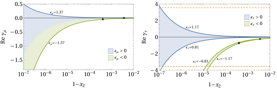
Figure 1: The possible values of the real parts of the Yukawa couplings $\gamma_{\mu}$ (left panel) and $\gamma_{\tau}$ (right panel) versus $1-x_{2}$, according to inequalities (53d) and (53b), respectively. In the right panel, the dashed orange lines indicate the upper bound $\left|\mathrm{Re}\,\gamma_{\tau}\right|\leq\sqrt{4\pi}\approx 3.5$ that we impose in our fits. The locations of the benchmark points of table 3 are marked by crosses (for BP-1) and stars (for BP-2).

We parameterize the vertex of $S_{2}^{0}$ with two charged scalars through Eq. (12). We already know from Eqs. (13) that

$$\lambda_{212}=\lambda_{122} = \frac{e\left(m_{H^{+}}^{2}-m_{h}^{2}\right)}{2s_{w}m_{W}}\,\sqrt{1-x_{2}^{2}},$$ (54a)

$$\lambda_{112} = -\frac{em_{h}^{2}}{2s_{w}m_{W}}\,x_{2}.$$ (54b)

The value of $\lambda_{222}$, i.e. of the coupling $H^{-}H^{+}S_{2}^{0}$, depends on the scalar potential. If we write the quartic part of the scalar potential of the 2HDM in the standard notation [70]

$$V_{4} = \frac{\lambda_{1}}{2}\left(\Phi_{1}^{\dagger}\Phi_{1}\right)^{2}+\frac{\lambda_{2}}{2}\left(\Phi_{2}^{\dagger}\Phi_{2}\right)^{2}+\lambda_{3}\,\Phi_{1}^{\dagger}\Phi_{1}\,\Phi_{2}^{\dagger}\Phi_{2}+\lambda_{4}\,\Phi_{1}^{\dagger}\Phi_{2}\,\Phi_{2}^{\dagger}\Phi_{1}$$ (55)

$$+\left[\frac{\lambda_{5}}{2}\left(\Phi_{1}^{\dagger}\Phi_{2}\right)^{2}+\left(\lambda_{6}\Phi_{1}^{\dagger}\Phi_{1}+\lambda_{7}\Phi_{2}^{\dagger}\Phi_{2}\right)\Phi_{1}^{\dagger}\Phi_{2}+\mathrm{H.c.}\right],$$

then [64]

$$\lambda_{222}=-\frac{2s_{w}m_{W}}{e}\left(x_{2}\lambda_{3}+\sqrt{1-x_{2}^{2}}\ \mathrm{Re}\,\lambda_{7}\right).$$ (56)

The coupling $\lambda_{222}$ is important for $S_{2}^{0}\to\ell_{1}^{+}\ell_{2}^{-}$; there is a diagram for that decay wherein $S_{2}^{0}$ attaches to $H^{-}H^{+}$. However, in practice that diagram gives amplitudes (D5) that are always much smaller than the dominant amplitudes (D4) and (D11). We have found that, for $-1<\lambda_{3}<7$ and $\left|\mathrm{Re}\,\lambda_{7}\right|<1.5$ [71], the branching ratios $\mathrm{BR}\left(S_{2}^{0}\to\ell_{1}^{+}\ell_{2}^{-}\right)$ are almost completely independent of $\lambda_{222}$. Thereafter we have kept $\lambda_{3}=\mathrm{Re}\,\lambda_{7}=1$ fixed.

2.4 Fit to the lepton-mixing data

The lepton mixing matrix $U$ is in the charged-current Lagrangian (34). It is a $3\times 6$ matrix. We must connect it to the standard PMNS $3\times 3$ unitary matrix. In order to make this connection we use the seesaw approximation [72, 73, 74, 75, 76], which is valid when the eigenvalues of $M_{R}$ are very much larger than the (diagonal) matrix elements of $M_{D}$. The $3\times 3$ symmetric matrix

$$\mathcal{M}_{\nu}=-M_{D}^{T}M_{R}^{-1}M_{D}$$ (57)

is diagonalized by an unitary matrix $V$ as

$$V^{T}\mathcal{M}_{\nu}V=\mathrm{diag}\left(n_{1},n_{2},n_{3}\right):=\hat{n},$$ (58)

where the $n_{p}$ ($p=1,2,3$) are real and positive. It follows from Eqs. (57) and (58) that

$$M_{R}=-M_{D}V\hat{n}^{-1}V^{T}M_{D}^{T}.$$ (59)

In our fitting program we input the PMNS matrix $V$, the Yukawa couplings $d_{e,\mu,\tau}$, and the $n_{p}$. We firstly write the matrix $M_{D}$ given by Eq. (47). We then determine $M_{R}$ through Eq. (59). We use $M_{R}$ and $M_{D}$ to construct the $6\times 6$ matrix

$$\left(\begin{array}[]{cc}0_{3\times 3}&M_{D}^{T}\\ M_{D}&M_{R}\end{array}\right).$$ (60)

We diagonalize the matrix (60) through the unitary matrix $U_{6}$ as in Eq. (30). We thus find both $U$, viz. the $3\times 6$ upper submatrix of $U_{6}$, and the neutrino masses $m_{i}$ ($i=1,\ldots,6$). Because the seesaw approximation is very good, one obtains $m_{i}\approx n_{i}$ for $i=1,2,3$ and moreover the $3\times 3$ left submatrix of $U$ turns out approximately equal to $V$. Finally, we order the heavy-neutrino masses as $m_{4}\leq m_{5}\leq m_{6}$.

Since the inputted $n_{p}$ are many orders of magnitude below the Fermi scale, the matrix elements of $M_{R}$ are much above the Fermi scale unless the Yukawa couplings $d_{\ell}$ are extremely small. Therefore, when we lower the inputted $d_{\ell}$, we lower the heavy-neutrino masses.

For the $n_{p}$ we use the light-neutrino masses. The cosmological bound [77] is

$$\sum_{p=1}^{3}n_{p}\approx\sum_{\mathrm{light\,neutrinos}}m_{\nu}<0.12\,\mathrm{eV},$$ (61)

together with the squared-mass differences $\Delta_{\mathrm{solar}}=n_{2}^{2}-n_{1}^{2}$ and $\Delta_{\mathrm{atmospheric}}=\left|n_{3}^{2}-n_{1}^{2}\right|$, that are taken from phenomenology. The lightest-neutrino mass is kept free; we let it vary in between $10^{-5}$ eV and $\sim 0.03$ eV for normal ordering ($n_{1}<n_{3}$), and in between $10^{-5}$ eV and $\sim 0.015$ eV for inverted ordering ($n_{3}<n_{1}$); the upper bound on the lightest-neutrino mass is indirectly provided by the cosmological bound (61). The smallest $n_{p}$ cannot be allowed to be zero because $\hat{n}^{-1}$ appears in Eq. (59). For the matrix $V$ we use the parameterization [66]

$$V=\left(\begin{array}[]{ccc}c_{12}c_{13}&s_{12}c_{13}&\epsilon^{\ast}\\ -s_{12}c_{23}-c_{12}s_{23}\epsilon&c_{12}c_{23}-s_{12}s_{23}\epsilon&s_{23}c_{13}\\ s_{12}s_{23}-c_{12}c_{23}\epsilon&-c_{12}s_{23}-s_{12}c_{23}\epsilon&c_{23}c_{13}\end{array}\right)\times\mathrm{diag}\left(1,\ e^{i\alpha_{21}/2},\ e^{i\alpha_{31}/2}\right),$$ (62)

where $\epsilon\equiv s_{13}\exp{\left(i\delta\right)}$, $c_{pq}=\cos{\theta_{pq}}$, and $s_{pq}=\sin{\theta_{pq}}$ for $(pq)=(12),(13),(23)$.

Three different groups [78, 79, 80] have derived, from the data provided by various neutrino-oscillation experiments, values for the mixing angles $\theta_{pq}$, for the phase $\delta$, and for $\Delta_{\mathrm{solar}}$ and $\Delta_{\mathrm{atmospheric}}$. The results of the three groups (especially the $1\sigma$ bounds) are different, but in Ref. [78] the values of the observables are in between the bounds of Refs. [79] and [80]. In this paper we use the $3\sigma$ data from Ref. [78] that are summarised in table 2.

Quantity	Best fit	x 1$\sigma$ range x	x 3$\sigma$ range x
$\Delta_{\mathrm{solar}}\left/\left(10^{-5}\mathrm{eV}^{2}\right)\right.$ $1^{1^{1^{a}}}$	7.55	7.39–7.75	7.05–8.14
$\Delta_{\mathrm{atmospheric}}\left/\left(10^{-3}\mathrm{eV}^{2}\right)\right.$ (NO)	2.50	2.47–2.53	2.41–2.60
$\Delta_{\mathrm{atmospheric}}\left/\left(10^{-3}\mathrm{eV}^{2}\right)\right.$ (IO)	2.42	2.34–2.47	2.31-2.51
$\sin^{2}\theta_{12}\left/10^{-1}\right.$	3.20	3.04–3.40	2.73–3.79
$\sin^{2}\theta_{23}\left/10^{-1}\right.$ (NO)	5.47	5.17–5.67	4.45–5.99
$\sin^{2}\theta_{23}\left/10^{-1}\right.$ (IO)	5.51	5.21–5.69	4.53–5.98
$\sin^{2}\theta_{13}\left/10^{-2}\right.$ (NO)	2.160	2.091–2.243	1.96–2.41
$\sin^{2}\theta_{13}\left/10^{-2}\right.$ (IO)	2.220	2.144–2.146	1.99–2.44
$\delta\left/\mathrm{rad}\right.$ (NO)	3.80	3.33–4.46	2.73–6.09
$\delta\left/\mathrm{rad}\right.$ (IO)	4.90	4.43–5.31	3.52–6.09

Table 2: The neutrino-oscillation parameters used in our fits [78].

The Majorana phases $\alpha_{21}$ and $\alpha_{31}$ are kept free in our analysis.

3 Numerical results

3.1 Details of the computation

We have generated the complete set of diagrams for each process in Feynman gauge by using the package FeynMaster [81] (that package combines FeynRules [82, 83], QGRAF [84], and FeynCalc [85, 86]) with a modified version of the FeynRules Standard-Model file to account for the six neutrinos, for lepton flavour mixing, and for the additional Higgs doublet. The amplitudes generated automatically by FeynMaster were expressed through Passarino–Veltman (PV) functions by using the package FeynCalc and specific functions of FeynMaster. All the amplitudes were checked by performing the computations manually. The results of these computations are presented in Appendices B, C, and D.

For numerical calculations we made two separate programs, one with Mathematica and another one with Fortran. Because of the very large differences among

the mass scale of the light neutrinos, between $10^{-5}$ eV and $0.1$ eV,

the mass scale of the charged leptons, between $100$ keV and $1$ GeV,

and the mass scale of the heavy neutrinos, between $100$ GeV and $10^{16}$ GeV,

there are both numerical instabilities and delicate cancellations in the calculations. These numerical problems could be solved with the high-precision numbers that Mathematica allows. However, this strongly slows down the calculations. Fortunately, numerical inaccuracies occur only for very small values (less than $10^{-30}$) of the branching ratios (BRs), therefore we were able to use a program written with Fortran to implement the minimization procedure and to find BRs within ranges relevant to experiment. Some parts of the Fortran code (such as the module for matrix diagonalization) have used quadruple precision to avoid inaccuracies, but most of the code has used just double precision so that the computational speed was sufficient for minimization. The final results were checked with the high precision afforded by Mathematica.

The numerical computation of the PV functions was performed by using the Fortran library Collier [87], which is designed for the numerical evaluation of one-loop scalar and tensor integrals. A major advantage of Collier over the LoopTools package [88] is that it avoids numerical instabilities when the neutrino masses are very large, even when one only uses double precision. The integrals were checked with Mathematica’s high-precision numbers and Package-X [89] analytic expressions of one-loop integrals.

In the fits of subsection 3.4, in order to find adequate numerical values for the parameters we have constructed a $\chi^{2}$ function to be minimized:

$$\chi^{2}=\sum_{i=1}^{n}\left[\Theta\left(O_{i}^{b}-O_{i}^{v}\right)\left(\frac{O_{i}^{b}}{O_{i}^{v}}\right)^{2}+\Theta\left(O_{i}^{v}-O_{i}^{b}\right)\left(\frac{O_{i}^{v}-O_{i}^{b}}{k}\right)^{2}\right].$$ (63)

In Eq. (63),

• $n$ is the total number of observables to be fitted; this is usually nine, since we fit the BRs of the nine LFV decays in order to find them within the ranges accessible to experiment.

• $\Theta$ is the Heaviside step function.

• $O_{i}^{v}$ is the computed value of each observable.

• $O_{i}^{b}$ is the experimental upper bound on the observable, which is given in table 1.

• $k$ is an appropriately small number that short-circuits the minimization algorithm when $O_{i}^{v}$ turns out larger than $O_{i}^{b}$.

The $\chi^{2}$ function (63) works well even when the calculated BRs and the experimental upper bounds differ by many orders of magnitude. We have performed the fits in subsection 3.4 by minimizing $\chi^{2}$ with respect to the model parameters—the Yukawa couplings $d_{\ell}$, $\delta_{\ell}$, and $\gamma_{\ell}$, and the PMNS-matrix parameters. The mass of the lightest neutrino and the parameter $x_{2}$ were randomly generated before the minimization of the $\chi^{2}$ function, in order to be able to explore the full range of the neutrino masses and the full range of $x_{2}$. In the fits of subsection 3.4 the mass of the charged scalar $H^{+}$ was usually kept fixed, just as the parameters $\lambda_{3}$ and $\mathrm{Re}\,\lambda_{7}$ of the scalar potential (55).

The minimization of $\chi^{2}$ is not an easy task because of the large number of model parameters that, moreover, may differ by several orders of magnitude, and because there is always a large number of local minima. However, we don’t try to find absolute minima, i.e. BRs as close as possible to the experimental upper bound; our purpose is rather to search under which circumstances the decay rates may be in experimentally accessible ranges.

The inputted values of the masses of the leptons and bosons were taken from Ref. [66]. We have used $s_{w}^{2}=0.22337$ and $e\equiv\sqrt{4\pi\alpha}$, where $\alpha=1/137.036$ is the fine-structure constant. The neutrino-oscillation data are in table 2.

We introduce the shorthands BR($\ell$), BR($Z$), and BR($h$) for the branching ratios of the decays $\ell_{1}^{\pm}\to\ell_{2}^{\pm}\gamma$, $Z\to\ell_{1}^{\pm}\ell_{2}^{\mp}$, and $h\to\ell_{1}^{\pm}\ell_{2}^{\mp}$, respectively. We also define the lower bound $Y_{\mathrm{min}}=10^{-6}$ and the upper bound $Y_{\mathrm{max}}=\sqrt{4\pi}\approx 3.5$ on the moduli of the Yukawa coupling constants.

3.2 Benchmark points

We produce in table 3 two benchmark points (BPs). For those two BPs the neutrino mass ordering is normal, the neutrino squared-mass differences and the lepton mixing angles take their best-fit values in table 2, the mass of the charged scalar is 750 GeV, and the parameters $\lambda_{3}$ and $\lambda_{7}$ of the scalar potential are both equal to 1.

	Point 1 (BP-1)	Point 2 (BP-2)
$d_{e}$	$10^{-6}$	$0.25$
$d_{\mu}$	$4\times 10^{-6}$	$0.7$
$d_{\tau}$	$10^{-6}$	$0.4$
$\delta_{e}$	$3.5$	$0.7$
$\delta_{\mu}$	$3.5$	$0.2$
$\delta_{\tau}$	$3.5$	$0.7$
$\gamma_{e}$	$0.3$	$0.3$
$\gamma_{\mu}$	$10^{-4}$	– $0.043$
$\gamma_{\tau}$	– $0.24$	– $0.73$
$\kappa_{\mu}$	$1.01$	– $1.04$
$\kappa_{\tau}$	– $1.04$	– $1.06$
$m_{1}$ (meV)	16.5	5.2
$\alpha_{21}$ (rad)	$3.515$	0
$\alpha_{31}$ (rad)	$1.060$	0
$1-x_{2}$	$0.0036$	$0.0004$
$m_{4}$ (TeV)	$1.16066$	$1.33740\times 10^{11}$
$m_{5}$ (TeV)	$3.54866$	$3.07494\times 10^{11}$
$m_{6}$ (TeV)	$6.67826$	$12.5369\times 10^{11}$
$\mathrm{BR}\left(\tau^{\pm}\to\mu^{\pm}\gamma\right)\times 10^{9}$	$8.1$	—
$\mathrm{BR}\left(\tau^{\pm}\to e^{\pm}\gamma\right)\times 10^{9}$	$12$	—
$\mathrm{BR}\left(\mu^{\pm}\to e^{\pm}\gamma\right)\times 10^{13}$	$2.2$	—
$\mathrm{BR}\left(Z\to\tau^{\pm}\mu^{\mp}\right)\times 10^{13}$	$9.6$	—
$\mathrm{BR}\left(Z\to\tau^{\pm}e^{\mp}\right)\times 10^{13}$	$12$	—
$\mathrm{BR}\left(Z\to\mu^{\pm}e^{\mp}\right)\times 10^{15}$	$38$	—
$\mathrm{BR}\left(h\to\tau^{\pm}\mu^{\mp}\right)\times 10^{4}$	$3.6$	$5.5$
$\mathrm{BR}\left(h\to\tau^{\pm}e^{\mp}\right)\times 10^{4}$	$5.5$	$8.9$
$\mathrm{BR}\left(h\to\mu^{\pm}e^{\mp}\right)\times 10^{5}$	$3.6$	$3.9$

Table 3: Two benchmark points. In the third column, the symbol ‘—’ stands for a tiny number $\lesssim 10^{-20}$. The values of the input parameters absent from the first column are given at the beginning of subsection 3.2.

The first nine rows of table 3 contain the inputted values of the Yukawa couplings; the next two lines have the computed values of $\kappa_{\mu}$ and $\kappa_{\tau}$; in the next four lines one finds the inputted values of the lightest-neutrino mass $m_{1}$, of the Majorana phases $\alpha_{21}$ and $\alpha_{31}$, and of the non-alignment parameter $1-x_{2}$; the next three lines have the computed masses of the heavy neutrinos, ordered as $m_{4}\leq m_{5}\leq m_{6}$; the last nine lines display the computed branching ratios.

In benchmark point 2 (BP-2) only the BR($h$) are sufficiently large to be observed in the future, while the BR($\ell$) and BR($Z$) are negligibly small. Benchmark point 1 (BP-1) indicates that very small values of the Yukawa couplings $d_{\ell}$ and large values of the Yukawa couplings $\delta_{\ell}$ are required in order to obtain BR($\ell$) in experimentally reachable ranges. BP-2 shows that, if only the BR($h$) are accessible, then the Yukawa couplings may all be in the range $\left[0.1,\ 1\right]$; in that case, since the $d_{\ell}$ are not very small, the heavy-neutrino masses are quite large.

3.3 Evolution of BRs

In this subsection we discuss the behaviour of the BRs when we vary some input parameters of the benchmark point 1 of the previous section, while the other input parameters of that point remain fixed.

In order to visualize the impact of the Yukawa coupling constants on the BRs, we have fixed their ratios in the same way as in BP-1, viz.

$$d_{\tau}=d_{e},\qquad d_{\mu}=4\,d_{\tau},\qquad\delta_{e}=\delta_{\mu}=\delta_{\tau},\qquad\frac{0.3\,\gamma_{\tau}}{\gamma_{e}}=\frac{\gamma_{\tau}}{10^{4}\,\gamma_{\mu}}=-0.24.$$ (64)

We change either only $d_{\tau}$, or only $\delta_{\tau}$, or only $\gamma_{\tau}$, and we let the other Yukawa couplings vary together with them through the fixed ratios (64). All the other input parameters keep the values of BP-1.

In Fig. 2 we display the BRs against $d_{\tau}$,

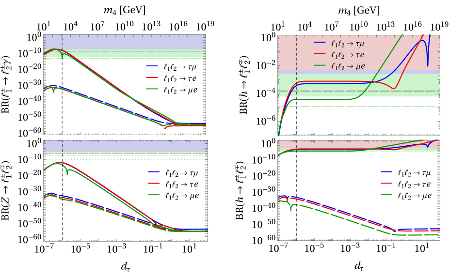
Figure 2: The branching ratios as functions of the Yukawa coupling $d_{\tau}$. Full lines give the BRs computed with the contribution of all amplitudes; dashed lines represent the BRs computed only with the amplitudes that do not involve the charged scalars $H^{\pm}$. The shadowed bands are excluded by the present experimental data; the dashed/dotted horizontal lines show the future experimental sensitivities given in table 1. The colours of the shadowed bands coincide with the colours of the lines, viz. blue for $\left(\ell_{1},\,\ell_{2}\right)=\left(\tau,\,\mu\right)$, red for $\left(\ell_{1},\,\ell_{2}\right)=\left(\tau,\,e\right)$, and green for $\left(\ell_{1},\,\ell_{2}\right)=\left(\mu,\,e\right)$. The vertical dashed lines mark the location of BP-1 of table 3. The upper-right panel is a zoom of the upper part of the bottom-right one. In the left panels, the blue lines almost always coincide with the red ones.

while the three $\delta_{\ell}$ and the three $\gamma_{\ell}$ are kept equal to their respective values of BP-1. It should be noted, in the upper and lower horizontal scales of Fig. 2, that the mass $m_{4}$ of the lightest heavy neutrino varies as $m_{4}\propto d_{\tau}^{2}$. One observes, in the top-left panel of Fig. 2, that the BR($\ell$) reach values close to their experimental upper bounds for a narrow range of $d_{\tau}$, viz. $2\times 10^{-7}\lesssim d_{\tau}\lesssim 8\times 10^{-6}$; for these tiny values of $d_{\tau}$, $m_{4}\lesssim 10^{4}$ GeV. The behaviour of the BR($Z$) is shown in the bottom-left panel of Fig. 2; it is similar to the behaviour of the BR($\ell$), as one might foresee from the similarities in the amplitudes for the two processes, cf. appendices B and C. Unfortunately, however, because of a small factor in the decay width, cf. Eq. (C2), the predicted BR($Z$) are smaller by more than six orders of magnitude than the present experimental upper bounds.

We observe a completely different behaviour of the BR($h$) in the right panels of Fig. 2 (the top panel is a zoom of part of the bottom one): the BR($h$) achieve values comparable to the experimental upper bounds for a wide range of $d_{\tau}$, viz. even when the heavy-neutrino masses are quite large.

The main message of Fig. 2 is that all nine BRs would be very small if there were no charged scalars $H^{\pm}$. The contributions to the amplitudes from the diagrams with $H^{\pm}$ increase some BRs in some circumstances by several orders of magnitude.

The BRs behave differently when plotted against the Yukawa couplings $\delta_{\ell}$, as shown in Fig. 3.

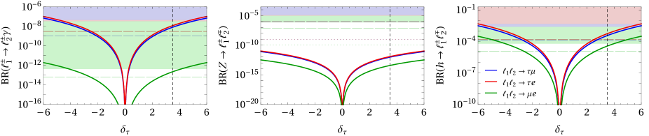
Figure 3: The branching ratios as functions of the Yukawa couplings $\delta_{\tau}=\delta_{\mu}=\delta_{e}$. See the caption of Fig. 2 for further explanations.

We see that all the BRs increase with increasing absolute value of $\delta_{\ell}$; the BR($\ell$) and BR($h$) become visible in planned experiments when $\left|\delta_{\ell}\right|\gtrsim 2$ (for appropriate values of the other parameters, especially very small $d_{\ell}$, as they are in Fig. 3). With decreasing $\left|\delta_{\ell}\right|$ the BRs decrease monotonically for all decays because of the decreasing values of all the amplitudes; when $\left|\delta_{\tau}\right|\sim 10^{-6}$ the BRs have minimum values somewhere between $10^{-35}$ and $10^{-25}$.

The dependence of the BR($\ell$) and BR($Z$) from the Yukawa couplings $\gamma_{\ell}$ is weak, as shown in the left panel of Fig. 4.

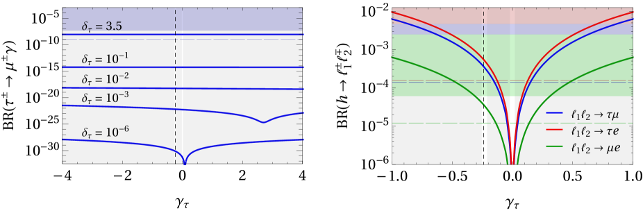
Figure 4: Some branching ratios as functions of the Yukawa coupling $\gamma_{\tau}$. The vertical dashed lines mark the value $\gamma_{\tau}=-0.24$ of benchmark point 1. Left panel: $\mathrm{BR}\left(\tau^{\pm}\to\mu^{\pm}\gamma\right)$ versus $\gamma_{\tau}$ for various values of $\delta_{\tau}$. Right panel: the BR($h$) versus $\gamma_{\tau}$ for $\delta_{\tau}=3.5$. The light-gray-shadowed bands are regions excluded by the inequalities (53).

The reason for this is that in the dominant amplitudes, viz. the ones in Eq. (B14), the $d_{\ell}$ and $\delta_{\ell}$ have much stronger impact than the $\gamma_{\ell}$. The relevance of the $\gamma_{\ell}$ is much stronger on BR($h$); in the right panel of Fig. 4 one sees that experimentally visible BR($h$) may be reached when $\left|\gamma_{\tau}\right|\gtrsim 0.1$, for appropriate values of the other parameters. The BR($h$) decrease with decreasing $\left|\gamma_{\ell}\right|$ because of the decreasing values of the dominant amplitudes, viz. $d_{l/rb,\mathrm{16}}$ in Eq. (D4) and $d_{l/rb,\mathrm{19}}$ in Eqs. (D11). However, for $\left|\gamma_{\tau}\right|\lesssim 10^{-3}$ the amplitudes $d_{l/rb,\mathrm{17}}$ in Eq. (D5) become dominant and the BR($h$) do not decrease much any further.

In Figs. 2 and 4 we have seen that the behaviour of BR($h$) is different from the one of BR($Z$) and BR($\ell$). This happens because of different amplitudes, but also because of additional parameters, viz. $x_{2}$ and the triple-scalar couplings $\lambda_{3}$ and $\lambda_{7}$, that arise in the diagram of Fig. 17 where $h$ attaches to two charged scalars with couplings given by Eqs. (54) and (56). However, due to the small factor $\sqrt{1-x_{2}^{2}}$ in the second term of Eq. (56), the impact of $\lambda_{7}$ on BR($h$) is almost imperceptible. On the other hand, $\lambda_{3}$ may have a strong influence on BR($h$). This happens only for extremely small values of $1-x_{2}$, though; and, for such extremely small values of $1-x_{2}$, BR($h$) is anyway much too small to be measurable. This is displayed in Fig. 5. In the cases that we are interested in, viz. when the BR($h$) are rather large, the exact value of $\lambda_{3}$ is unimportant.

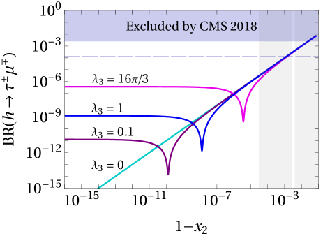
Figure 5: $\mathrm{BR}\left(h\to\tau^{\pm}\mu^{\mp}\right)$ versus $1-x_{2}$ for various values of the triple-scalar coupling $\lambda_{3}$; all the other input parameters are as in BP-1. The bands shadowed in light gray are excluded by inequalities (53). The vertical dashed line marks the value $1-x_{2}=0.0036$ of BP-1.

For the sake of simplicity, from now one we assume $\lambda_{3}=\lambda_{7}=1$ everywhere.

With decreasing $1-x_{2}$, the BRs in Fig. 5 decrease because of the decreasing dominant amplitudes $d_{l/rb,\mathrm{16}}$ in Eq. (D4) and $d_{l/rb,\mathrm{19}}$ in Eqs. (D11). At some point, though, the amplitudes $d_{l/rb,\mathrm{17}}$ in Eqs. (D5) begin to dominate and then the BRs do not decrease much any further. The dips in the lines of Fig. 5 arise from the partial cancellation of amplitudes $d_{l/rb,\mathrm{16}}$ and $d_{l/rb,\mathrm{19}}$ with the amplitudes $d_{l/rb,\mathrm{17}}$.

As shown in Fig. 5, $1-x_{2}$ has a strong impact on BR($h$). It is also important for making BR($h$) and BR($\ell$) simultaneously close to the experimental bounds. Indeed, the BR($h$) may be made sufficiently large, for a wide range of the Yukawa couplings $d_{\ell}$ and for sufficiently large values of the $\delta_{\ell}$, just by varying $1-x_{2}$. The strong impact of $1-x_{2}$ and of the $\gamma_{\ell}$ on BR($h$) allows one to adjust BR($h$), together with BR($\ell$), to be close to the experimental upper bounds—but for a quite restricted range of $d_{\ell}$ and $\delta_{\ell}$, because large BR($\ell$) require extremely small $d_{\ell}$ and rather large $\delta_{\ell}$. If, on the other hand, one attempts to fit only BR($h$), then both $1-x_{2}$ and the Yukawa couplings may be much more relaxed, as shown in BP-2 of table 3.

In Fig. 6 we illustrate the evolution of the BRs when the mass of the charged scalar $m_{H^{+}}$ is changed, while the other parameters are kept fixed at their values of BP-1.

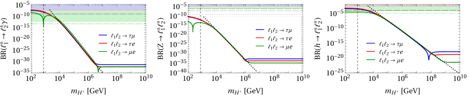
Figure 6: The decay rates versus the mass of the charged scalar $m_{H^{+}}$; all the other parameters are kept at their values of benchmark point 1 in table 3. The vertical dashed lines mark $m_{H^{+}}=750$ GeV. The oblique dashed lines are given by Eqs. (65).

One observes that when $m_{H^{+}}$ increases the BRs mostly decrease monotonically as (for the other parameters fixed in their values of BP-1)

$$\mathrm{BR}\left(\ell\right) \approx 10^{17.72}\left(\frac{m_{H^{+}}}{1\,\mathrm{GeV}}\right)^{-7.51},$$ (65a)

$$\mathrm{BR}\left(Z\right) \approx 10^{13.82}\left(\frac{m_{H^{+}}}{1\,\mathrm{GeV}}\right)^{-7.82},$$ (65b)

$$\mathrm{BR}\left(h\right) \approx 10^{10.47}\left(\frac{m_{H^{+}}}{1\,\mathrm{GeV}}\right)^{-3.58}.$$ (65c)

Eventually, when $m_{H^{+}}\sim 10^{7}$ GeV for BR($\ell$) and BR($Z$), and when $m_{H^{+}}\sim 10^{9}$ GeV for BR($h$), the BRs settle at their SM values. This illustrates the decoupling of $H^{+}$. One also sees in Fig. 6 that, for $\left(\ell_{1},\ell_{2}\right)=\left(\mu,e\right)$, there is near $m_{H^{+}}=750$ GeV a partial cancellation of amplitudes that leads to a sudden drop of $\mathrm{BR}\left(\mu^{\pm}\to e^{\pm}\gamma\right)$; our benchmark point 1 has profited from that effect for attaining $\mathrm{BR}(\mu^{\pm}\to e^{\pm}\gamma)$ smaller than its experimental upper bound.

In Fig. 7 we display the BRs as functions of the Majorana phase $\alpha_{31}$, with the other input parameters kept fixed at their values of BP-1.

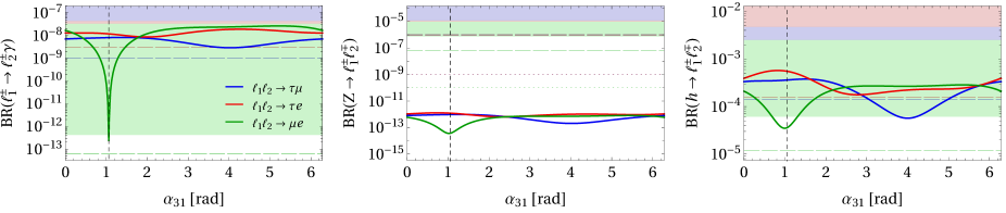
Figure 7: The decay rates versus the Majorana phase $\alpha_{31}$; all the other parameters are kept at their values of benchmark point 1 of table 3. The vertical dashed lines mark the value $\alpha_{31}=1.06$ of BP-1.

Here too, for $\left(\ell_{1},\ell_{2}\right)=\left(\mu,e\right)$ there is a sudden drop of the branching ratios when $\alpha_{31}=1.06$, which is precisely the value that we have utilized in benchmark point 1. A similar behaviour of the green lines also occurs with other parameters, besides $m_{H^{+}}$ (Fig. 6) and $\alpha_{31}$ (Fig. 7). Hence, the values of the parameters must be chosen very carefully if we want to find all six BR($\ell$) and BR($h$) simultaneously close to their experimental upper bounds. The main difficulty arises because the upper bound on $\mathrm{BR}\left(\mu^{\pm}\to e^{\pm}\gamma\right)$ differs from the upper bound on $\mathrm{BR}\left(\tau^{\pm}\to\mu^{\pm}\gamma\right)$ by five orders of magnitude. Fortunately, our minimization procedure allows this to be done quite efficiently.

3.4 Fitting the BRs

In this model there is a large number of input parameters. We have performed a minimization procedure in order to find adequate values for all of them. For each set of input parameters, we have computed the branching ratios of the nine LFV decays; we have then selected sets of input parameters for which all six BR($\ell$) and BR($h$) are simultaneously between the current experimental upper bounds and the future experimental sensitivities.

Since in this subsection we use a fitting procedure, we must enforce definite bounds on the input parameters, lest they acquire either much too small or much too large values. We adopt the following conditions:

• The neutrino-oscillation parameters, viz. the mixing angles $\theta_{12}$, $\theta_{13}$, and $\theta_{23}$, the Dirac phase $\delta$, and the neutrino squared-mass differences, are varied within their respective $3\sigma$ ranges taken from Ref. [78] and reproduced in table 2. The Majorana phases $\alpha_{21}$ and $\alpha_{31}$ are kept free, i.e. we let them vary from 0 to $2\pi$.

• The lightest-neutrino mass is varied in between $10^{-5}$ eV and either $\sim 0.03$ eV for normal ordering of the neutrino masses or $\sim 0.015$ eV for inverted ordering. The precise upper bound on the lightest neutrino mass is fixed, for each pair of values of $\Delta_{\mathrm{solar}}$ and $\Delta_{\mathrm{atmospheric}}$, by the Planck 2018 cosmological upper bound (61).

• The Yukawa coupling constants $d_{\ell}$, $\delta_{\ell}$, and $\gamma_{\ell}$ are assumed to be real (either positive or negative).

• The moduli of the Yukawa coupling constants are varied between $Y_{\mathrm{min}}=10^{-6}$ (which is the order of magnitude of the Yukawa coupling of the electron) and a perturbativity bound $Y_{\mathrm{max}}=\sqrt{4\pi}\approx 3.5$.

• We enforce Eqs. (53).

There are experimental and phenomenological constraints on the mass of the charged scalar $m_{H^{+}}$, as discussed in Appendix F. The numerical study in the previous subsection (see Fig. 6) shows that, when $m_{H^{+}}$ increases, most BRs decrease. Since we attempt to obtain largish BRs, the fitting procedure always tends to produce the lowest $m_{H^{+}}$ in the allowed range. In our fits we have fixed $m_{H^{+}}=750$ GeV, in agreement with the lower bounds of recent global fits [90, 91]. We have also kept the triple-scalar couplings fixed, viz. $\lambda_{3}=\lambda_{7}=1$, because they do not change much the BRs. Finally, we have checked that all the final points meet the $3\sigma$ conditions on the $Z$ invisible decay width in Eq. (E6).

In the figures of this subsection we display three different fits:

1. In the first fit (displayed through blue points and called ‘NO’ from now on), we have assumed normal ordering of the light-neutrino masses.

2. In the second fit (displayed through red points and named ‘IO’) there is inverted ordering of the light-neutrino masses.

3. In the numerical analysis we have found that most points have $\left|d_{\ell}\right|$ close to the lower bound $Y_{\mathrm{min}}=10^{-6}$. Therefore, we have produced a third fit (displayed through green points and labelled ‘$Y_{\mathrm{min}}=10^{-7}$’) that has normal ordering like the first one, but where the lower bound on the moduli of the Yukawa couplings is $10^{-7}$ instead of $10^{-6}$.

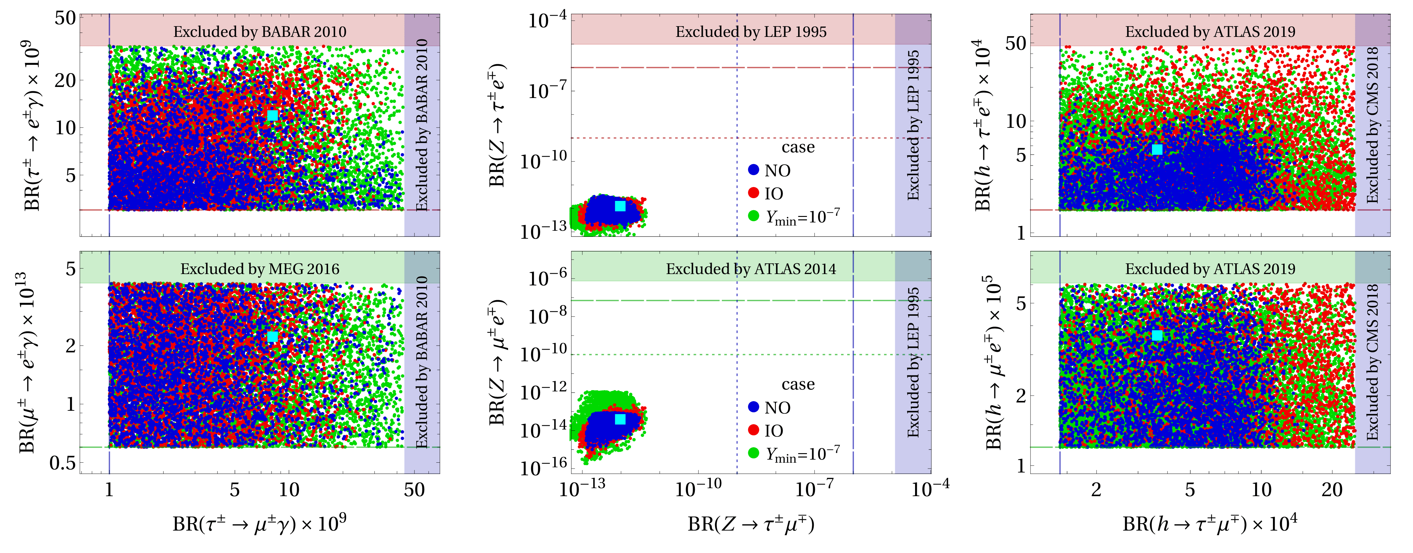
Figure 8: Scatter plots of the branching ratios for three different fits. Blue points have normal ordering of the light-neutrino masses, red points have inverted ordering, and green points have a lower bound ($10^{-7}$ instead of $10^{-6}$) on the moduli of the Yukawa couplings. A cyan square marks BP-1 of table 3. The shadowed bands are the present experimental upper bounds on the BRs; dashed and/or dotted lines show the future experimental sensitivities, as described in table 1.

Figure 8 shows that points for the NO and IO cases are similarly distributed in what respects the BR($\ell$) and BR($Z$). It is possible in both cases to find points with the BR($\ell$) close to the experimental upper bounds, while the BR($Z$) always remain much too suppressed. For the BR($h$), on the other hand, NO usually leads to smaller values than IO. The larger freedom of the third fit (with $Y_{\mathrm{min}}=10^{-7}$ instead of $Y_{\mathrm{min}}=10^{-6}$) facilitates larger BR($\ell$), as shown by the green points in Fig. 8.

Most points in Fig. 8 have negative $\kappa_{\tau}$. This allows larger $\mathrm{BR}\left(h\to\tau^{\pm}\mu^{\mp}\right)$ and $\mathrm{BR}\left(h\to\tau^{\pm}e^{\mp}\right)$. If one only allows positive $\kappa_{\tau}$, then in NO it is not possible to reach the future sensitivity for $\mathrm{BR}\left(h\to\tau^{\pm}\mu^{\mp}\right)$, except if one allows complex Yukawa couplings. On the other hand, in both the IO and $Y_{\mathrm{min}}=10^{-7}$ cases it is still possible to get all three BR($h$) above their future sensitivities with positive $\kappa_{\mu}$ and $\kappa_{\tau}$.

We have found that free Majorana phases permit larger BRs for the decays with $\tau^{\pm}$. Thus, it is advantageous to fit the Majorana phases instead of fixing them at any pre-assigned values.

In Fig. 9 we display correlation plots of BR($\ell$) and BR($Z$).

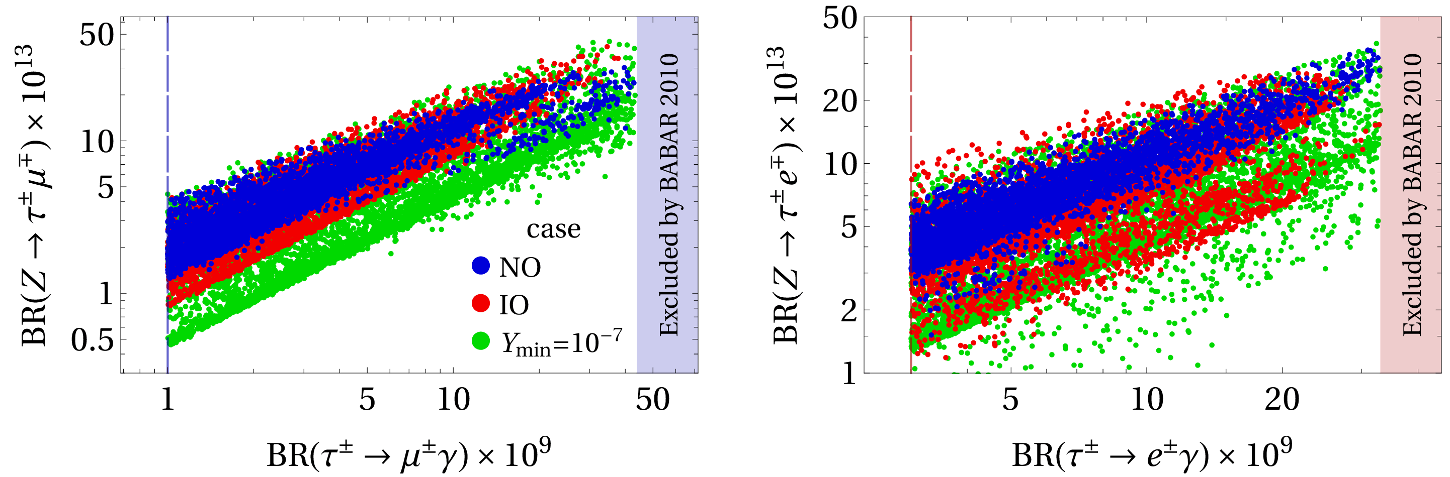
Figure 9: Correlation plots between BR($\ell$) and BR($Z$) for the three fits of Fig. 8; the points and the notation are the same as in that figure.

One sees that there is a correlation between $\mathrm{BR}\left(\tau^{\pm}\to\mu^{\pm}\gamma\right)$ and $\mathrm{BR}\left(Z\to\tau^{\pm}\mu^{\mp}\right)$, and a correlation between $\mathrm{BR}\left(\tau^{\pm}\to e^{\pm}\gamma\right)$ and $\mathrm{BR}\left(Z\to\tau^{\pm}e^{\mp}\right)$. These correlations are one of the main reasons for the small BR($Z$) in our model; if we want to keep the BR($\ell$) below their experimental upper bounds, then we necessarily obtain much too low BR($Z$). Indeed, one sees in Fig. 9 that the BABAR 2010 upper bounds on the BR($\tau$) lead, in our model, to $\mathrm{BR}\left(Z\to\tau^{\pm}\mu^{\mp}\right)\lesssim 6\times 10^{-12}$ and $\mathrm{BR}\left(Z\to\tau^{\pm}e^{\mp}\right)\lesssim 4\times 10^{-12}$; those values are much lower than the future experimental sensitivity. We point out that in other models (see for instance Refs. [24], [41], and [42]) there are also correlations between the BR($Z$) and BR($\ell$), and also with the branching ratios for three-body LFV decays $\ell^{\pm}_{1}\to\ell^{\pm}_{2}\ell^{+}_{3}\ell^{-}_{3}$.

In some models there are correlations between $\mathrm{BR}\left(h\to\tau^{\pm}\mu^{\mp}\right)$ and either [46, 48, 49, 57] $\mathrm{BR}\left(\tau^{\pm}\to\mu^{\pm}\gamma\right)$ or [50] $\mathrm{BR}\left(\mu^{\pm}\to e^{\pm}\gamma\right)$. In our model we did not find correlations between the BR($\ell$) and BR($h$).

In Fig. 10 we display histograms of the moduli of the Yukawa couplings for our three fits.

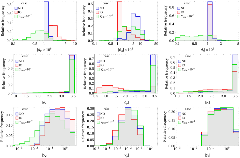
Figure 10: The distributions of the moduli of the Yukawa couplings for the three fits.

In the first row of panels one sees that, in order to get BR($\ell$) in experimentally reachable ranges, our fits always have very small $\left|d_{\ell}\right|\lesssim 10^{-5}$. If we had set $Y_{\mathrm{min}}$ much larger than $10^{-6}$, then it might not have been possible to obtain BR($\ell$) visible in the next generation of experiments. In the fit with relaxed $Y_{\mathrm{min}}=10^{-7}$ the distribution of the $\left|d_{\ell}\right|$ is more uniform. The second row of Fig. 10 shows that, in all three fits, $\left|\delta_{e,\mu,\tau}\right|$ have values close to the allowed upper bound $Y_{\mathrm{max}}$. In the third row one sees that the $\left|\gamma_{e,\mu,\tau}\right|$ vary in rather wide ranges, from $\sim 10^{-4}$ to $Y_{\mathrm{max}}$. This happens because the parameter $1-x_{2}$ has a strong impact on BR($h$); for smaller values of the $\gamma_{\ell}$, larger values of $1-x_{2}$ still allow BR($h$) to reach experimentally reachable ranges.

In Fig. 11 we display the heavy-neutrino masses $m_{4}$, $m_{5}$, and $m_{6}$ for our three fits.

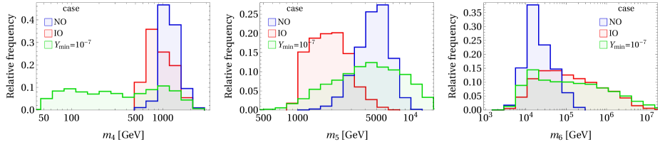
Figure 11: Histograms of the heavy-neutrino masses for the three fits.

Because the $\left|d_{\ell}\right|$ are always so small in the fits, the heavy-neutrino masses are very small too. Thus, in NO and IO $m_{4}$ lies in between $\sim 0.5$ TeV and $\sim 2.5$ TeV, and in $Y_{\mathrm{min}}=10^{-7}$ it may be as small as 45 GeV. The mass $m_{5}$ is in between $\sim 1$ TeV and $\sim 10$ TeV for all cases, and the mass $m_{6}$ is in between $\sim 2.5$ TeV and $\sim 100$ TeV for NO, and $\sim 10^{4}$ TeV for both IO and $Y_{\mathrm{min}}=10^{-7}$.

In all three fits, it is found that the mixing angles $\theta_{12,23,13}$, the Dirac phase $\delta$, and the Majorana phases $\alpha_{21}$ and $\alpha_{31}$ may have values anywhere in their ranges.

3.5 Single decays

In the previous subsection we have discussed the results that are obtained when all six BR($\ell$) and BR($h$) are simultaneously between the current experimental upper bounds and the future experimental sensitivities. Here we consider the case where only one of those six BRs is above the future sensitivity.

We have found that requiring just one BR($\ell$) to be above the future sensitivity still restricts the Yukawa couplings $\left|d_{\ell}\right|\lesssim 10^{-3}$ and $\left|\delta_{\ell}\right|\gtrsim 0.5$. Then, because of the small $\left|d_{\ell}\right|$, the heavy-neutrino mass $m_{4}$ is always of order 1 TeV (except in $\mu^{\pm}\to e^{\pm}\gamma$ for which $m_{4}$ may be of order 50 TeV).

Requiring just one BR($h$) to be above the future sensitivity restricts $\left|\delta_{\ell}\right|\gtrsim 0.1$. The $\left|d_{\ell}\right|$ and the heavy-neutrino masses do not need to be very small, as one sees for instance in BP-2 of table 3.

In our model the decay $Z\to\mu^{\pm}e^{\mp}$ might be observed at the FCC-ee collider in a very restricted range of circumstances, viz. with large $\left|\delta_{e,\mu}\right|\gtrsim 4$, small $\left|d_{e}\right|\lesssim 10^{-6}$ and $\left|d_{\mu,\tau}\right|\lesssim 5\times 10^{-6}$, and small $m_{H^{+}}\lesssim 500$ GeV. Moreover, a very precise finetuning is required, wherein the Yukawa couplings are such that on the hand the decay $\mu^{\pm}\to e^{\pm}\gamma$ has a cancellation of amplitudes leading to its BR being below the experimental upper bound, and on the other hand $\mathrm{BR}\left(Z\to\mu^{\pm}e^{\mp}\right)$ still remains a little above the FCC-ee sensitivity. The other two LFV $Z$ decays $Z\to\tau^{\pm}e^{\mp}$ and $Z\to\tau^{\pm}\mu^{\mp}$ are in our model always much too suppressed to be visible.

3.6 Amplitudes

Numerically, we have found that only a few amplitudes have a substantial impact on the BRs.

For $\ell_{1}^{\pm}\to\ell_{2}^{\pm}\gamma$ the amplitudes (B14) are dominant. Specifically, $a_{l,H}$ in Eq. (B14a) gives the main impact. Therefore, the approximate decay width is

$$\Gamma\left(\ell_{1}^{\pm}\to\ell_{2}^{\pm}\gamma\right)\approx\frac{m_{\ell_{1}}^{4}-m_{\ell_{2}}^{4}}{16\pi m_{\ell_{1}}^{3}}\,\left|\mathcal{S}\,e\right|^{2}\left|a_{l,H}\right|^{2}.$$ (66)

This yields the following approximate formulas for the BRs:

$$\mathrm{BR}\left(\tau^{\pm}\to\mu^{\pm}\gamma\right) \approx \left(5.733\times 10^{4}\right)\left|a_{l,H}\right|^{2},$$ (67a)

$$\mathrm{BR}\left(\tau^{\pm}\to e^{\pm}\gamma\right) \approx \left(5.733\times 10^{4}\right)\left|a_{l,H}\right|^{2},$$ (67b)

$$\mathrm{BR}\left(\mu^{\pm}\to e^{\pm}\gamma\right) \approx \left(2.580\times 10^{10}\right)\left|a_{l,H}\right|^{2}.$$ (67c)

The amplitude $\bar{a}_{l,H}$ in Eq. (C9a) is the most important one for the BR($Z$).  Therefore,

$$\Gamma\left(Z\to\ell_{1}^{\pm}\ell_{2}^{\mp}\right) \approx \frac{\sqrt{m_{Z}^{4}-2m_{Z}^{2}\left(m_{\ell_{1}}^{2}+m_{\ell_{2}}^{2}\right)+\left(m_{\ell_{1}}^{2}-m_{\ell_{2}}^{2}\right)^{2}}}{48\pi m_{Z}^{5}}\,$$ (68)

$$\times\left|\mathcal{S}\,e\right|^{2}\left[2m_{Z}^{4}-m_{Z}^{2}\left(m_{\ell_{1}}^{2}+m_{\ell_{2}}^{2}\right)-\left(m_{\ell_{1}}^{2}-m_{\ell_{2}}^{2}\right)^{2}\right]\left|\bar{a}_{l,H}\right|^{2}.$$

Hence,

$$\mathrm{BR}\left(Z\to\ell_{1}^{\pm}\ell_{2}^{\mp}\right)\approx\left(1.781\times 10^{-6}\right)\left|\bar{a}_{l,H}\right|^{2}.$$ (69)

The amplitudes for the Higgs decays differ from those for the other decays. The amplitudes from the self-energy-like diagrams of Fig. 16, with the charged scalar $H^{\pm}$, give the strongest impact on the branching ratios. Specifically, the amplitude $d_{rb,\mathrm{16(a,b)}}$ in Eq. (D4b) is significant for largish values of the Yukawa couplings $d_{\ell}$ and the amplitude $d_{lb,\mathrm{16(a,b)}}$ in Eq. (D4a) is significant for all values of the $d_{\ell}$. Moreover, for the $h$ decays the amplitudes from diagrams with two internal neutrino lines, depicted in Fig. 19, are important too. Specifically, the amplitudes $d_{lb,\mathrm{19(a)}}$ and $d_{rb,\mathrm{19(a)}}$ are relevant. Thus, defining

$$\bar{d}_{lb}=d_{lb,\mathrm{16(a,b)}}+d_{lb,\mathrm{19(a)}},\quad\quad\bar{d}_{rb}=d_{rb,\mathrm{16(a,b)}}+d_{rb,\mathrm{19(a)}},$$ (70)

we have

$$\mathrm{BR}\left(h\to\tau^{\pm}\mu^{\mp}\right) \approx \left(2.451\times 10^{-2}\right)\left(\left|\bar{d}_{lb}\right|^{2}+\left|\bar{d}_{rb}\right|^{2}\right)$$ (71a)

$$-\left(1.176\times 10^{-6}\right)\mathrm{Re}\left(\bar{d}_{lb}\bar{d}_{rb}^{\ast}\right),$$

$$\mathrm{BR}\left(h\to\tau^{\pm}e^{\mp}\right) \approx \left(2.451\times 10^{-2}\right)\left(\left|\bar{d}_{lb}\right|^{2}+\left|\bar{d}_{rb}\right|^{2}\right)$$ (71b)

$$-\left(5.690\times 10^{-9}\right)\mathrm{Re}\left(\bar{d}_{lb}\bar{d}_{rb}^{\ast}\right),$$

$$\mathrm{BR}\left(h\to\mu^{\pm}e^{\mp}\gamma\right) \approx \left(2.452\times 10^{-2}\right)\left(\left|\bar{d}_{lb}\right|^{2}+\left|\bar{d}_{rb}\right|^{2}\right)$$ (71c)

$$-\left(3.384\times 10^{-10}\right)\mathrm{Re}\left(\bar{d}_{lb}\bar{d}_{rb}^{\ast}\right).$$

In order to check the correctness of the approximate BRs of Eqs. (67), (69), and (71) we have calculated the asymmetry between the exact BRs and the approximate ones,

$$\mathrm{BR}_{\mathrm{asymmetry}}\equiv\frac{\left|\mathrm{BR}_{\mathrm{exact}}-\mathrm{BR}_{\mathrm{approximate}}\right|}{\mathrm{BR}_{\mathrm{exact}}+\mathrm{BR}_{\mathrm{approximate}}}.$$ (72)

Using the points of case ‘NO’, these asymmetries are displayed in Fig. 12.

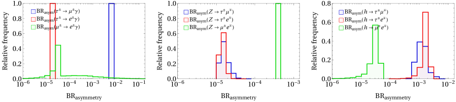
Figure 12: Histograms of the asymmetries between the exact nine branching ratios and their approximate expressions in Eqs. (67), (69), and (70)–(71).

One sees that $\mathrm{BR}_{\mathrm{asymmetry}}\lesssim 0.1$, which means that the approximate formulas are quite accurate. These approximate expressions for the BRs may be very useful for intermediate calculations of the fitting procedure, where the calculations need to be repeated many times, before the final result is calculated by using the exact expressions. This computational trick has saved us a lot of time.

4 Summary and conclusions

Here we summarize our main findings:

• The amplitudes with the charged scalar are crucial in order to obtain $\mathrm{BR}\left(\ell_{1}^{\pm}\to\ell_{2}^{\pm}\gamma\right)$ and $\mathrm{BR}\left(h\to\ell_{1}^{\pm}\ell_{2}^{\mp}\right)$ in experimentally accessible ranges.

• Because the experimental upper bound on $\mathrm{BR}\left(\mu^{\pm}\to e^{\pm}\gamma\right)$ is very small, it is often necessary to finetune the values of the input parameters of the model so that the largest amplitudes for that specific decay partially cancel among themselves, while the other five decays $\ell_{1}^{\pm}\to\ell_{2}^{\pm}\gamma$ and $h\to\ell_{1}^{\pm}\ell_{2}^{\mp}$ remain experimentally visible in the future.

• The decays $\ell_{1}^{\pm}\to\ell_{2}^{\pm}\gamma$ necessitate large values of the Yukawa couplings $\left|\delta_{\ell}\right|\gtrsim 1$ and extremely small values of the Yukawa couplings $\left|d_{\ell}\right|\lesssim 10^{-5}$ in order to be visible. The latter imply a very low seesaw scale, i.e. rather light right-handed neutrinos.

• In our model the decays $Z\to\ell_{1}^{\pm}\ell_{2}^{\mp}$ correlate with the decays $\ell_{1}^{\pm}\to\ell_{2}^{\pm}\gamma$, i.e. they behave similarly as functions of the parameters. Because of this correlation, the experimental upper bounds on $\mathrm{BR}\left(\ell_{1}^{\pm}\to\ell_{2}^{\pm}\gamma\right)$ imply that the decays $Z\to\ell_{1}^{\pm}\ell_{2}^{\mp}$ will remain invisible in all the planned experiments.

• The decays $h\to\ell_{1}^{\pm}\ell_{2}^{\mp}$ behave quite differently from $\ell_{1}^{\pm}\to\ell_{2}^{\pm}\gamma$ and $Z\to\ell_{1}^{\pm}\ell_{2}^{\mp}$. They might be visible in future experiments without the need to choose either very large or very small Yukawa couplings.

• The Majorana phases have a significant impact on the branching ratios of all the decays. One should refrain from fixing them at any pre-assigned values.

• Both normal and inverted ordering of the light-neutrino masses may yield decay rates of adequate orders of magnitude.

• When the mass of the charged scalar increases, most BRs decrease. Still, for $m_{H^{+}}\lesssim 1.5$ TeV the decays $\ell_{1}^{\pm}\to\ell_{2}^{\pm}\gamma$ and $h\to\ell_{1}^{\pm}\ell_{2}^{\mp}$ might be visible in future experiments.

Acknowledgements:

D.J. thanks both Jorge C. Romão and Duarte Fontes for useful discussions. He also thanks the Lithuanian Academy of Sciences for financial support through projects DaFi2019 and DaFi2021; he was also supported by a COST STSM grant through action CA16201. L.L. warmly thanks the Institute of Theoretical Physics and Astronomy of the University of Vilnius for the hospitality extended during a visit where part of this work has been done. L.L. also thanks the Portuguese Foundation for Science and Technology for support through projects CERN/FIS-PAR/0004/2019, CERN/FIS-PAR/0008/2019, PTDC/FIS-PAR/29436/2017, UIDB/00777/2020, and UIDP/00777/2020.

Appendix A Passarino–Veltman functions

The relevant Passarino–Veltman (PV) functions are defined in the following way. Let the dimension of space–time be $d=4-\epsilon$ with $\epsilon\to 0$. We define

$$\mathcal{D}k:=\mu^{\epsilon}\,\frac{\mathrm{d}^{d}k}{\left(2\pi\right)^{d}},\quad\quad\mathcal{S}:=\frac{i}{16\pi^{2}}.$$ (A1)

Then,

$$\int\mathcal{D}k\ \frac{1}{k^{2}-A}\ \frac{1}{\left(k+p\right)^{2}-B} = \mathcal{S}\,B_{0}\left(p^{2},A,B\right),$$ (A2a)

$$\int\mathcal{D}k\ k^{\theta}\,\frac{1}{k^{2}-A}\ \frac{1}{\left(k+p\right)^{2}-B} = \mathcal{S}\,p^{\theta}\,B_{1}\left(p^{2},A,B\right),$$ (A2b)

and

$$\int\mathcal{D}k\ \frac{1}{k^{2}-A}\ \frac{1}{\left(k+p\right)^{2}-B}\ \frac{1}{\left(k+q\right)^{2}-C} = \mathcal{S}\,C_{0}\left[p^{2},\left(p-q\right)^{2},q^{2},A,B,C\right],$$ (A3a)

$$\int\mathcal{D}k\ k^{\theta}\,\frac{1}{k^{2}-A}\ \frac{1}{\left(k+p\right)^{2}-B}\ \frac{1}{\left(k+q\right)^{2}-C} = \mathcal{S}\left\{p^{\theta}\,C_{1}\left[p^{2},\left(p-q\right)^{2},q^{2},A,B,C\right]\right.$$

$$\left.+q^{\theta}\,C_{2}\left[p^{2},\left(p-q\right)^{2},q^{2},A,B,C\right]\right\},$$

$$\int\mathcal{D}k\ k^{\theta}k^{\psi}\,\frac{1}{k^{2}-A}\ \frac{1}{\left(k+p\right)^{2}-B}\ \frac{1}{\left(k+q\right)^{2}-C} = \mathcal{S}\left\{p^{\theta}p^{\psi}\,C_{11}\left[p^{2},\left(p-q\right)^{2},q^{2},A,B,C\right]\right.$$

$$+q^{\theta}q^{\psi}\,C_{22}\left[p^{2},\left(p-q\right)^{2},q^{2},A,B,C\right]$$

$$+\left(p^{\theta}q^{\psi}+q^{\theta}p^{\psi}\right)C_{12}\left[p^{2},\left(p-q\right)^{2},q^{2},\right.$$

$$\left.A,B,C\right]$$

$$\left.+g^{\theta\psi}\,C_{00}\left[p^{2},\left(p-q\right)^{2},q^{2},A,B,C\right]\right\}.$$

Some PV functions in Eqs. (A2) and (A3) have $1\!\left/\epsilon\right.$ divergences that are independent of the arguments of the PV functions. Thus,

$$B_{0}\left(p^{2},A,B\right) = \frac{2}{\epsilon}+\mathrm{finite\ terms},$$ (A4a)

$$B_{1}\left(p^{2},A,B\right) = -\frac{1}{\epsilon}+\mathrm{finite\ terms},$$ (A4b)

$$C_{00}\left[p^{2},\left(p-q\right)^{2},q^{2},A,B,C\right] = \frac{1}{2\epsilon}+\mathrm{finite\ terms}.$$ (A4c)

All other PV functions in Eqs. (A2) and (A3) converge when $\epsilon\to 0$.

We next introduce specific notations for some PV functions that are used in appendices B, C, and D. Thus,

$$e_{0} := C_{0}\left(m_{\ell_{1}}^{2},q^{2},m_{\ell_{2}}^{2},m_{i}^{2},m_{a}^{2},m_{a}^{2}\right),$$ (A5a)

$$e_{1} := C_{1}\left(m_{\ell_{1}}^{2},q^{2},m_{\ell_{2}}^{2},m_{i}^{2},m_{a}^{2},m_{a}^{2}\right),$$ (A5b)

$$e_{2} := C_{2}\left(m_{\ell_{1}}^{2},q^{2},m_{\ell_{2}}^{2},m_{i}^{2},m_{a}^{2},m_{a}^{2}\right),$$ (A5c)

$$e_{11} := C_{11}\left(m_{\ell_{1}}^{2},q^{2},m_{\ell_{2}}^{2},m_{i}^{2},m_{a}^{2},m_{a}^{2}\right),$$ (A5d)

$$e_{22} := C_{22}\left(m_{\ell_{1}}^{2},q^{2},m_{\ell_{2}}^{2},m_{i}^{2},m_{a}^{2},m_{a}^{2}\right),$$ (A5e)

$$e_{12} := C_{12}\left(m_{\ell_{1}}^{2},q^{2},m_{\ell_{2}}^{2},m_{i}^{2},m_{a}^{2},m_{a}^{2}\right),$$ (A5f)

$$e_{00} := C_{00}\left(m_{\ell_{1}}^{2},q^{2},m_{\ell_{2}}^{2},m_{i}^{2},m_{a}^{2},m_{a}^{2}\right),$$ (A5g)

$$f_{0} := C_{0}\left(m_{\ell_{1}}^{2},q^{2},m_{\ell_{2}}^{2},m_{i}^{2},m_{W}^{2},m_{W}^{2}\right),$$ (A6a)

$$f_{1} := C_{1}\left(m_{\ell_{1}}^{2},q^{2},m_{\ell_{2}}^{2},m_{i}^{2},m_{W}^{2},m_{W}^{2}\right),$$ (A6b)

$$f_{2} := C_{2}\left(m_{\ell_{1}}^{2},q^{2},m_{\ell_{2}}^{2},m_{i}^{2},m_{W}^{2},m_{W}^{2}\right),$$ (A6c)

$$f_{11} := C_{11}\left(m_{\ell_{1}}^{2},q^{2},m_{\ell_{2}}^{2},m_{i}^{2},m_{W}^{2},m_{W}^{2}\right),$$ (A6d)

$$f_{22} := C_{22}\left(m_{\ell_{1}}^{2},q^{2},m_{\ell_{2}}^{2},m_{i}^{2},m_{W}^{2},m_{W}^{2}\right),$$ (A6e)

$$f_{12} := C_{12}\left(m_{\ell_{1}}^{2},q^{2},m_{\ell_{2}}^{2},m_{i}^{2},m_{W}^{2},m_{W}^{2}\right),$$ (A6f)

$$f_{00} := C_{00}\left(m_{\ell_{1}}^{2},q^{2},m_{\ell_{2}}^{2},m_{i}^{2},m_{W}^{2},m_{W}^{2}\right),$$ (A6g)

$$g_{0} := C_{0}\left(m_{\ell_{1}}^{2},q^{2},m_{\ell_{2}}^{2},m_{a}^{2},m_{i}^{2},m_{j}^{2}\right),$$ (A7a)

$$g_{1} := C_{1}\left(m_{\ell_{1}}^{2},q^{2},m_{\ell_{2}}^{2},m_{a}^{2},m_{i}^{2},m_{j}^{2}\right),$$ (A7b)

$$g_{2} := C_{2}\left(m_{\ell_{1}}^{2},q^{2},m_{\ell_{2}}^{2},m_{a}^{2},m_{i}^{2},m_{j}^{2}\right),$$ (A7c)

$$g_{11} := C_{11}\left(m_{\ell_{1}}^{2},q^{2},m_{\ell_{2}}^{2},m_{a}^{2},m_{i}^{2},m_{j}^{2}\right),$$ (A7d)

$$g_{22} := C_{22}\left(m_{\ell_{1}}^{2},q^{2},m_{\ell_{2}}^{2},m_{a}^{2},m_{i}^{2},m_{j}^{2}\right),$$ (A7e)

$$g_{12} := C_{12}\left(m_{\ell_{1}}^{2},q^{2},m_{\ell_{2}}^{2},m_{a}^{2},m_{i}^{2},m_{j}^{2}\right),$$ (A7f)

$$g_{00} := C_{00}\left(m_{\ell_{1}}^{2},q^{2},m_{\ell_{2}}^{2},m_{a}^{2},m_{i}^{2},m_{j}^{2}\right),$$ (A7g)

$$h_{0} := C_{0}\left(m_{\ell_{1}}^{2},q^{2},m_{\ell_{2}}^{2},m_{W}^{2},m_{i}^{2},m_{j}^{2}\right),$$ (A8a)

$$h_{1} := C_{1}\left(m_{\ell_{1}}^{2},q^{2},m_{\ell_{2}}^{2},m_{W}^{2},m_{i}^{2},m_{j}^{2}\right),$$ (A8b)

$$h_{2} := C_{2}\left(m_{\ell_{1}}^{2},q^{2},m_{\ell_{2}}^{2},m_{W}^{2},m_{i}^{2},m_{j}^{2}\right),$$ (A8c)

$$h_{11} := C_{11}\left(m_{\ell_{1}}^{2},q^{2},m_{\ell_{2}}^{2},m_{W}^{2},m_{i}^{2},m_{j}^{2}\right),$$ (A8d)

$$h_{22} := C_{22}\left(m_{\ell_{1}}^{2},q^{2},m_{\ell_{2}}^{2},m_{W}^{2},m_{i}^{2},m_{j}^{2}\right),$$ (A8e)

$$h_{12} := C_{12}\left(m_{\ell_{1}}^{2},q^{2},m_{\ell_{2}}^{2},m_{W}^{2},m_{i}^{2},m_{j}^{2}\right),$$ (A8f)

$$h_{00} := C_{00}\left(m_{\ell_{1}}^{2},q^{2},m_{\ell_{2}}^{2},m_{W}^{2},m_{i}^{2},m_{j}^{2}\right),$$ (A8g)

$$j_{0} := C_{0}\left(m_{\ell_{1}}^{2},q^{2},m_{\ell_{2}}^{2},m_{i}^{2},m_{a}^{2},m_{a^{\prime}}^{2}\right),$$ (A9a)

$$j_{1} := C_{1}\left(m_{\ell_{1}}^{2},q^{2},m_{\ell_{2}}^{2},m_{i}^{2},m_{a}^{2},m_{a^{\prime}}^{2}\right),$$ (A9b)

$$j_{2} := C_{2}\left(m_{\ell_{1}}^{2},q^{2},m_{\ell_{2}}^{2},m_{i}^{2},m_{a}^{2},m_{a^{\prime}}^{2}\right),$$ (A9c)

$$k_{0} := C_{0}\left(m_{\ell_{1}}^{2},q^{2},m_{\ell_{2}}^{2},m_{i}^{2},m_{W}^{2},m_{a}^{2}\right),$$ (A10a)

$$k_{1} := C_{1}\left(m_{\ell_{1}}^{2},q^{2},m_{\ell_{2}}^{2},m_{i}^{2},m_{W}^{2},m_{a}^{2}\right),$$ (A10b)

$$k_{2} := C_{2}\left(m_{\ell_{1}}^{2},q^{2},m_{\ell_{2}}^{2},m_{i}^{2},m_{W}^{2},m_{a}^{2}\right),$$ (A10c)

$$k_{00} := C_{00}\left(m_{\ell_{1}}^{2},q^{2},m_{\ell_{2}}^{2},m_{i}^{2},m_{W}^{2},m_{a}^{2}\right),$$ (A10d)

$$k_{11} := C_{11}\left(m_{\ell_{1}}^{2},q^{2},m_{\ell_{2}}^{2},m_{i}^{2},m_{W}^{2},m_{a}^{2}\right),$$ (A10e)

$$k_{22} := C_{22}\left(m_{\ell_{1}}^{2},q^{2},m_{\ell_{2}}^{2},m_{i}^{2},m_{W}^{2},m_{a}^{2}\right),$$ (A10f)

$$k_{12} := C_{12}\left(m_{\ell_{1}}^{2},q^{2},m_{\ell_{2}}^{2},m_{i}^{2},m_{W}^{2},m_{a}^{2}\right),$$ (A10g)

$$l_{0} := C_{0}\left(m_{\ell_{1}}^{2},q^{2},m_{\ell_{2}}^{2},m_{i}^{2},m_{a}^{2},m_{W}^{2}\right),$$ (A11a)

$$l_{1} := C_{1}\left(m_{\ell_{1}}^{2},q^{2},m_{\ell_{2}}^{2},m_{i}^{2},m_{a}^{2},m_{W}^{2}\right),$$ (A11b)

$$l_{2} := C_{2}\left(m_{\ell_{1}}^{2},q^{2},m_{\ell_{2}}^{2},m_{i}^{2},m_{a}^{2},m_{W}^{2}\right),$$ (A11c)

$$l_{00} := C_{00}\left(m_{\ell_{1}}^{2},q^{2},m_{\ell_{2}}^{2},m_{i}^{2},m_{a}^{2},m_{W}^{2}\right),$$ (A11d)

$$l_{11} := C_{11}\left(m_{\ell_{1}}^{2},q^{2},m_{\ell_{2}}^{2},m_{i}^{2},m_{a}^{2},m_{W}^{2}\right),$$ (A11e)

$$l_{22} := C_{22}\left(m_{\ell_{1}}^{2},q^{2},m_{\ell_{2}}^{2},m_{i}^{2},m_{a}^{2},m_{W}^{2}\right),$$ (A11f)

$$l_{12} := C_{12}\left(m_{\ell_{1}}^{2},q^{2},m_{\ell_{2}}^{2},m_{i}^{2},m_{a}^{2},m_{W}^{2}\right),$$ (A11g)

where $m_{\ell_{1}}$ and $m_{\ell_{2}}$ are the masses of the charged leptons $\ell_{1}^{\pm}$ and $\ell_{2}^{\pm}$, respectively, $m_{i}$ and $m_{j}$ are the masses of the neutrinos $\nu_{i}$ and $\nu_{j}$, respectively, $m_{a}$ and $m_{a^{\prime}}$ are the masses of the charged scalars $H_{a}^{\pm}$ and $H_{a^{\prime}}^{\pm}$, respectively, and $m_{W}$ is the mass of the gauge bosons $W^{\pm}$.

Appendix B $\ell_{1}^{\pm}\to\ell_{2}^{\pm}\gamma$

We compute the process $\ell_{1}^{-}\left(p_{1}\right)\to\ell_{2}^{-}\left(p_{2}\right)\gamma\left(q\right)$, where $q=p_{1}-p_{2}$. Obviously,

$$p_{1}^{2}=m_{\ell_{1}}^{2},\quad\quad p_{2}^{2}=m_{\ell_{2}}^{2},\quad\quad 2\,p_{1}\cdot p_{2}=m_{\ell_{1}}^{2}+m_{\ell_{2}}^{2}-q^{2}.$$ (B1)

If the outgoing photon is physical, then $q^{2}=0$; but we keep $q^{2}\neq 0$ for generality. The amplitude for a photon with polarization $\sigma$ is

$$T^{\sigma}=\mathcal{S}\,e\,\bar{u}_{\ell_{2}}\left(p_{2}\right)\left[\gamma^{\sigma}\left(a_{l}P_{L}+a_{r}P_{R}\right)+p_{1}^{\sigma}\left(b_{l}P_{L}+b_{r}P_{R}\right)+p_{2}^{\sigma}\left(c_{l}P_{L}+c_{r}P_{R}\right)\right]u_{\ell_{1}}\left(p_{1}\right),$$ (B2)

where $\mathcal{S}$ has been defined in Eq. (A1) and $e$ is the electric charge of the proton. Clearly,

$$\not\!p_{1}\,u_{\ell_{1}}\left(p_{1}\right)=m_{\ell_{1}}\,u_{\ell_{1}}\left(p_{1}\right),\quad\quad\overline{u}_{\ell_{2}}\left(p_{2}\right)\!\not\!p_{2}=m_{\ell_{2}}\,\overline{u}_{\ell_{2}}\left(p_{2}\right).$$ (B3)

If $T^{\sigma}$ in Eq. (B2) is multiplied by $q_{\sigma}$ and then Eqs. (B1) and (B3) are utilized, one must obtain zero because of gauge invariance. Thus,

$$2m_{\ell_{1}}a_{r}-2m_{\ell_{2}}a_{l}+\left(m_{\ell_{1}}^{2}-m_{\ell_{2}}^{2}\right)\left(b_{l}+c_{l}\right)+q^{2}\left(b_{l}-c_{l}\right) = 0,$$ (B4a)

$$2m_{\ell_{1}}a_{l}-2m_{\ell_{2}}a_{r}+\left(m_{\ell_{1}}^{2}-m_{\ell_{2}}^{2}\right)\left(b_{r}+c_{r}\right)+q^{2}\left(b_{r}-c_{r}\right) = 0.$$ (B4b)

We have used Eqs. (B4)—that hold even when $q^{2}\neq 0$—as a check on our calculations.

The decay width is, in the rest frame of the decaying $\ell_{1}^{-}$,

$$\Gamma=\frac{m_{\ell_{1}}^{2}-m_{\ell_{2}}^{2}}{16\pi m_{\ell_{1}}^{3}}\,\left|\mathcal{S}\,e\right|^{2}\left[\left(m_{\ell_{1}}^{2}+m_{\ell_{2}}^{2}\right)\left(\left|a_{l}\right|^{2}+\left|a_{r}\right|^{2}\right)-4\,m_{\ell_{1}}m_{\ell_{2}}\,\mathrm{Re}\left(a_{l}^{\ast}a_{r}\right)\right].$$ (B6)

In our model each of the coefficients $a_{l},\ldots,c_{r}$ is the sum of two contributions, viz.

$$a_{l}=a_{l,H}+a_{l,W},\quad\ldots,\quad c_{r}=c_{r,H}+c_{r,W}.$$ (B7)

The contributions with sub-index $H$ arise from the diagrams in Fig. 13 and are given in Eqs. (B14) below, and the contributions with sub-index $W$ come from the diagrams in Fig. 14 and are given in Eqs. (B22) below. Notice that Fig. 13 includes diagrams with the charged Goldstone bosons $G^{\pm}\equiv H_{1}^{\pm}$.

In all our calculations we utilize Feynman’s gauge. Let $m_{a}$ denote the mass of $H_{a}^{\pm}$; for $a=1$ one must use $m_{a=1}=m_{W}$ because we are in Feynman’s gauge.

B.1 $H_{a}^{\pm}$

The charged scalars $H_{a}^{\pm}$ couple to the charged leptons and the neutrinos according to Eq. (37). The charged scalars include as a particular case the charged Goldstone bosons. For $G^{\pm}=H_{1}^{\pm}$, one has [18]

$$R_{1\ell i}=\frac{e}{\sqrt{2}s_{w}m_{W}}\,U_{\ell i}m_{i},\quad\quad L_{1\ell i}=\frac{e}{\sqrt{2}s_{w}m_{W}}\,U_{\ell i}m_{\ell},$$ (B8)

where $U$ is the lepton mixing matrix and $s_{w}$ is the sine of the weak mixing angle.

The diagrams in Figs. 13(a) and 13(b) produce

Figure 13: The three diagrams for ${\ell_{1}}^{-}\to{\ell_{2}}^{-}\gamma$ with a loop containing $H_{a}^{\pm}$.

$$T_{\mathrm{13(a)}}^{\sigma}+T_{13(b)}^{\sigma} = \mathcal{S}\,e\,\sum_{i=1}^{6}\sum_{a=1}^{n}\left[\bar{u}_{\ell_{2}}\left(p_{2}\right)\gamma^{\sigma}\left(x_{ia}P_{R}+y_{ia}P_{L}\right)u_{\ell_{1}}\left(p_{1}\right)m_{\ell_{2}}\mathbf{b}_{0}\right.$$ (B9)

$$+\bar{u}_{\ell_{2}}\left(p_{2}\right)\gamma^{\sigma}\left(x_{ia}P_{L}+y_{ia}P_{R}\right)u_{\ell_{1}}\left(p_{1}\right)m_{\ell_{1}}\mathbf{b}_{0}$$

$$+\bar{u}_{\ell_{2}}\left(p_{2}\right)\gamma^{\sigma}\left(z_{ia}P_{L}+w_{ia}P_{R}\right)u_{\ell_{1}}\left(p_{1}\right)\mathbf{b}_{1}$$

$$\left.+\bar{u}_{\ell_{2}}\left(p_{2}\right)\gamma^{\sigma}\left(z_{ia}P_{R}+w_{ia}P_{L}\right)u_{\ell_{1}}\left(p_{1}\right)m_{\ell_{2}}m_{\ell_{1}}\mathbf{b}_{2}\right],$$

where

$$x_{ia} := R_{a{\ell_{2}}i}L^{\ast}_{a{\ell_{1}}i}m_{i},$$ (B10a)

$$y_{ia} := L_{a{\ell_{2}}i}R^{\ast}_{a{\ell_{1}}i}m_{i},$$ (B10b)

$$z_{ia} := R_{a{\ell_{2}}i}R^{\ast}_{a{\ell_{1}}i},$$ (B10c)

$$w_{ia} := L_{a{\ell_{2}}i}L^{\ast}_{a{\ell_{1}}i},$$ (B10d)

and

$$\mathbf{b}_{0} := \frac{B_{0}\left(m_{\ell_{1}}^{2},m_{i}^{2},m_{a}^{2}\right)-B_{0}\left(m_{\ell_{2}}^{2},m_{i}^{2},m_{a}^{2}\right)}{m_{\ell_{1}}^{2}-m_{\ell_{2}}^{2}},$$ (B11a)

$$\mathbf{b}_{1} := \frac{m_{\ell_{1}}^{2}\,B_{1}\left(m_{\ell_{1}}^{2},m_{i}^{2},m_{a}^{2}\right)-m_{\ell_{2}}^{2}B_{1}\left(m_{\ell_{2}}^{2},m_{i}^{2},m_{a}^{2}\right)}{m_{\ell_{1}}^{2}-m_{\ell_{2}}^{2}},$$ (B11b)

$$\mathbf{b}_{2} := \frac{B_{1}\left(m_{\ell_{1}}^{2},m_{i}^{2},m_{a}^{2}\right)-B_{1}\left(m_{\ell_{2}}^{2},m_{i}^{2},m_{a}^{2}\right)}{m_{\ell_{1}}^{2}-m_{\ell_{2}}^{2}}.$$ (B11c)

Notice that in our model

$$\sum_{i=1}^{6}z_{ia}=\sum_{i=1}^{6}R_{a\ell_{2}i}R_{a\ell_{1}i}^{\ast} = \sum_{k,k^{\prime}=1}^{n_{d}}\mathcal{U}_{ka}^{\ast}\mathcal{U}_{k^{\prime}a}\left(\Delta_{k}^{\dagger}\Delta_{k^{\prime}}\right)_{\ell_{2}\ell_{1}},$$ (B12a)

$$\sum_{i=1}^{6}w_{ia}=\sum_{i=1}^{6}L_{a\ell_{2}i}L_{a\ell_{1}i}^{\ast} = \sum_{k,k^{\prime}=1}^{n_{d}}\mathcal{U}_{ka}^{\ast}\mathcal{U}_{k^{\prime}a}\left(\Gamma_{k}\Gamma^{\dagger}_{k^{\prime}}\right)_{\ell_{2}\ell_{1}},$$ (B12b)

$$\sum_{i=1}^{6}x_{ia}=\sum_{i=1}^{6}R_{a\ell_{2}i}L_{a\ell_{1}i}^{\ast}m_{i} = \sum_{k,k^{\prime}=1}^{n_{d}}\mathcal{U}_{ka}^{\ast}\mathcal{U}_{k^{\prime}a}\left(\Delta_{k}^{\dagger}M_{D}\Gamma_{k^{\prime}}^{\dagger}\right)_{\ell_{2}\ell_{1}},$$ (B12c)

$$\sum_{i=1}^{6}y_{ia}=\sum_{i=1}^{6}L_{a\ell_{2}i}R_{a\ell_{1}i}^{\ast}m_{i} = \sum_{k,k^{\prime}=1}^{n_{d}}\mathcal{U}_{ka}^{\ast}\mathcal{U}_{k^{\prime}a}\left(\Gamma_{k}M_{D}^{\dagger}\Delta_{k^{\prime}}\right)_{\ell_{2}\ell_{1}}$$ (B12d)

vanish when $\ell_{2}\neq\ell_{1}$ by virtue of the matrices $\Gamma_{k}$, $\Delta_{k}$, and $M_{D}$ being diagonal.

The diagram 13(c) produces

$$T_{\mathrm{13(c)}}^{\sigma} = \mathcal{S}\,e\,\sum_{i=1}^{6}\sum_{a=1}^{n}\bar{u}_{\ell_{2}}\left(p_{2}\right)\left\{\left[\left(e_{0}+2e_{1}\right)p_{1}^{\sigma}+\left(e_{0}+2e_{2}\right)p_{2}^{\sigma}\right]\left(x_{ia}P_{R}+y_{ia}P_{L}\right)\right.$$ (B13)

$$+\left[\left(e_{2}+2e_{22}\right)p_{2}^{\sigma}+\left(e_{2}+2e_{12}\right)p_{1}^{\sigma}\right]m_{\ell_{2}}\left(z_{ia}P_{L}+w_{ia}P_{R}\right)$$

$$+\left[\left(e_{1}+2e_{11}\right)p_{1}^{\sigma}+\left(e_{1}+2e_{12}\right)p_{2}^{\sigma}\right]m_{\ell_{1}}\left(z_{ia}P_{R}+w_{ia}P_{L}\right)$$

$$\left.+2e_{00}\,\gamma^{\sigma}\left(z_{ia}P_{L}+w_{ia}P_{R}\right)\right\}u_{\ell_{1}}\left(p_{1}\right),$$

where the $e$ functions have been defined in Eqs. (A5).

Thus, adding Eqs. (B9) and (B13), one obtains

$$a_{l,H} = \sum_{i=1}^{6}\sum_{a=1}^{n}\left[\mathbf{b}_{0}m_{\ell_{1}}x_{ia}+\mathbf{b}_{0}m_{\ell_{2}}y_{ia}+\left(2e_{00}+\mathbf{b}_{1}\right)z_{ia}+\mathbf{b}_{2}m_{\ell_{2}}m_{\ell_{1}}w_{ia}\right],\hskip 19.91692pt$$ (B14a)

$$a_{r,H} = \sum_{i=1}^{6}\sum_{a=1}^{n}\left[\mathbf{b}_{0}m_{\ell_{2}}x_{ia}+\mathbf{b}_{0}m_{\ell_{1}}y_{ia}+\mathbf{b}_{2}m_{\ell_{2}}m_{\ell_{1}}z_{ia}+\left(2e_{00}+\mathbf{b}_{1}\right)w_{ia}\right],$$ (B14b)

$$b_{l,H} = \sum_{i=1}^{6}\sum_{a=1}^{n}\left[\left(e_{0}+2e_{1}\right)y_{ia}+\left(e_{2}+2e_{12}\right)m_{\ell_{2}}z_{ia}+\left(e_{1}+2e_{11}\right)m_{\ell_{1}}w_{ia}\right],$$ (B14c)

$$b_{r,H} = \sum_{i=1}^{6}\sum_{a=1}^{n}\left[\left(e_{0}+2e_{1}\right)x_{ia}+\left(e_{1}+2e_{11}\right)m_{\ell_{1}}z_{ia}+\left(e_{2}+2e_{12}\right)m_{\ell_{2}}w_{ia}\right],$$ (B14d)

$$c_{l,H} = \sum_{i=1}^{6}\sum_{a=1}^{n}\left[\left(e_{0}+2e_{2}\right)y_{ia}+\left(e_{2}+2e_{22}\right)m_{\ell_{2}}z_{ia}+\left(e_{1}+2e_{12}\right)m_{\ell_{1}}w_{ia}\right],$$ (B14e)

$$c_{r,H} = \sum_{i=1}^{6}\sum_{a=1}^{n}\left[\left(e_{0}+2e_{2}\right)x_{ia}+\left(e_{1}+2e_{12}\right)m_{\ell_{1}}z_{ia}+\left(e_{2}+2\,e_{22}\right)m_{\ell_{2}}w_{ia}\right].$$ (B14f)

One may use

$$B_{0}\left(m_{\ell_{1}}^{2},m_{i}^{2},m_{a}^{2}\right) = d\,e_{00}-m_{a}^{2}\,e_{0}+m_{\ell_{1}}^{2}\left(e_{1}+e_{11}+e_{12}\right)$$ (B15a)

$$+m_{\ell_{2}}^{2}\left(e_{0}+e_{1}+2\,e_{2}+e_{22}+e_{12}\right)-q^{2}\left(e_{1}+e_{12}\right),$$

$$B_{0}\left(m_{\ell_{2}}^{2},m_{i}^{2},m_{a}^{2}\right) = d\,e_{00}-m_{a}^{2}\,e_{0}+m_{\ell_{1}}^{2}\left(e_{0}+2\,e_{1}+e_{2}+e_{11}+e_{12}\right)$$ (B15b)

$$+m_{\ell_{2}}^{2}\left(e_{2}+e_{22}+e_{12}\right)-q^{2}\left(e_{2}+e_{12}\right),$$

$$B_{1}\left(m_{\ell_{1}}^{2},m_{i}^{2},m_{a}^{2}\right) = \left(m_{\ell_{2}}^{2}-m_{\ell_{1}}^{2}\right)\left(e_{1}+e_{11}+e_{12}\right)-2e_{00}+q^{2}\left(e_{12}-e_{11}\right),$$ (B15c)

$$B_{1}\left(m_{\ell_{2}}^{2},m_{i}^{2},m_{a}^{2}\right) = \left(m_{\ell_{1}}^{2}-m_{\ell_{2}}^{2}\right)\left(e_{2}+e_{22}+e_{12}\right)-2e_{00}+q^{2}\left(e_{12}-e_{22}\right),$$ (B15d)

where $d$ is the dimension of space–time, to derive

$$\mathbf{b}_{0} = -e_{0}-e_{1}-e_{2}+\frac{q^{2}}{m_{\ell_{1}}^{2}-m_{\ell_{2}}^{2}}\left(e_{2}-e_{1}\right),$$ (B16a)

$$2e_{00}+\mathbf{b}_{1} = -m_{\ell_{1}}^{2}\left(e_{1}+e_{11}\right)-m_{\ell_{2}}^{2}\left(e_{2}+e_{22}\right)+\left(q^{2}-m_{\ell_{1}}^{2}-m_{\ell_{2}}^{2}\right)e_{12}$$ (B16b)

$$+\frac{q^{2}}{m_{\ell_{1}}^{2}-m_{\ell_{2}}^{2}}\left(m_{\ell_{2}}^{2}\,e_{22}-m_{\ell_{1}}^{2}\,e_{11}\right),$$

$$\mathbf{b}_{2} = -e_{1}-e_{2}-e_{11}-e_{22}-2e_{12}+\frac{q^{2}}{m_{\ell_{1}}^{2}-m_{\ell_{2}}^{2}}\left(e_{22}-e_{11}\right).\hskip 19.91692pt$$ (B16c)

As a consequence of Eqs. (B16), the constraints (B4) hold for the contributions with sub-index $H$.

B.2 $W^{\pm}$

Besides the diagrams exclusively with $G^{\pm}$, there are five diagrams with $W^{\pm}$, cf. Fig. 14.

Figure 14: The five diagrams for ${\ell_{1}}^{-}\to{\ell_{2}}^{-}\gamma$ with a loop containing $W^{\pm}$.

Figures 14(d) and 14(e) have the outgoing photon attaching to $W^{\pm}G^{\mp}$. Those diagrams produce

$$a_{l,de} = -\frac{e^{2}}{2s_{w}^{2}}\,\sum_{i=1}^{6}U_{{\ell_{2}}i}U_{{\ell_{1}}i}^{\ast}\left(2m_{i}^{2}f_{0}+m_{\ell_{1}}^{2}f_{1}+m_{\ell_{2}}^{2}f_{2}\right),$$ (B17a)

$$a_{r,de} = \frac{e^{2}m_{\ell_{2}}m_{\ell_{1}}}{2s_{w}^{2}}\,\sum_{i=1}^{6}U_{{\ell_{2}}i}U_{{\ell_{1}}i}^{\ast}\left(f_{1}+f_{2}\right),$$ (B17b)

$$b_{l,de} = -\frac{e^{2}m_{\ell_{2}}}{s_{w}^{2}}\,\sum_{i=1}^{6}U_{{\ell_{2}}i}U_{{\ell_{1}}i}^{\ast}f_{1},$$ (B17c)

$$b_{r,de} = 0,$$ (B17d)

$$c_{l,de} = 0,$$ (B17e)

$$c_{r,de} = -\frac{e^{2}m_{\ell_{1}}}{s_{w}^{2}}\,\sum_{i=1}^{6}U_{{\ell_{2}}i}U_{{\ell_{1}}i}^{\ast}f_{2},$$ (B17f)

where the $f$ functions have been defined in Eqs. (A6). The diagram of Fig. 14(c) produces

$$a_{l,c} = \frac{e^{2}}{2s_{w}^{2}}\,\sum_{i=1}^{6}U_{{\ell_{2}}i}U_{{\ell_{1}}i}^{\ast}\left[\left(3m_{\ell_{1}}^{2}+2m_{\ell_{2}}^{2}-2q^{2}\right)f_{1}+\left(2m_{\ell_{1}}^{2}+3m_{\ell_{2}}^{2}-2q^{2}\right)f_{2}\right.$$ (B18a)

$$\left.+2m_{\ell_{1}}^{2}f_{11}+2m_{\ell_{2}}^{2}f_{22}+2\left(m_{\ell_{1}}^{2}+m_{\ell_{2}}^{2}-q^{2}\right)f_{12}+12f_{00}\right],\hskip 22.76219pt$$

$$a_{r,c} = \frac{3e^{2}m_{\ell_{2}}m_{\ell_{1}}}{2s_{w}^{2}}\,\sum_{i=1}^{6}U_{{\ell_{2}}i}U_{{\ell_{1}}i}^{\ast}\left(f_{1}+f_{2}\right),$$ (B18b)

$$b_{l,c} = -\frac{e^{2}m_{\ell_{2}}}{s_{w}^{2}}\,\sum_{i=1}^{6}U_{{\ell_{2}}i}U_{{\ell_{1}}i}^{\ast}\left(f_{1}+f_{2}-2f_{12}\right),$$ (B18c)

$$b_{r,c} = \frac{e^{2}m_{\ell_{1}}}{s_{w}^{2}}\,\sum_{i=1}^{6}U_{{\ell_{2}}i}U_{{\ell_{1}}i}^{\ast}\left(f_{1}+2f_{11}\right),$$ (B18d)

$$c_{l,c} = \frac{e^{2}m_{\ell_{2}}}{s_{w}^{2}}\,\sum_{i=1}^{6}U_{{\ell_{2}}i}U_{{\ell_{1}}i}^{\ast}\left(f_{2}+2f_{22}\right),$$ (B18e)

$$c_{r,c} = -\frac{e^{2}m_{\ell_{1}}}{s_{w}^{2}}\,\sum_{i=1}^{6}U_{{\ell_{2}}i}U_{{\ell_{1}}i}^{\ast}\left(f_{1}+f_{2}-2f_{12}\right).$$ (B18f)

A crucial property of the lepton mixing matrix $U$ in our model is

$$\left(UU^{\dagger}\right)_{\ell_{2}\ell_{1}}=\sum_{i=1}^{6}U_{{\ell_{2}}i}\,U_{{\ell_{1}}i}^{\ast}=0,$$ (B19)

cf. Eq. (29). In spite of $f_{00}$ containing a divergence $1\!\left/\left(2\epsilon\right)\right.$, $a_{l,c}$ in Eq. (B18a) is finite because of Eq. (B19).

Finally, there are the diagrams of Figs. 14(a) and 14(b), producing

$$a_{l,ab} = \frac{e^{2}}{s_{w}^{2}}\,\sum_{i=1}^{6}U_{{\ell_{2}}i}U_{{\ell_{1}}i}^{\ast}\mathbf{b}_{4},$$ (B20a)

$$a_{r,ab} = \frac{e^{2}m_{\ell_{2}}m_{\ell_{1}}}{s_{w}^{2}}\,\sum_{i=1}^{6}U_{{\ell_{2}}i}U_{{\ell_{1}}i}^{\ast}\mathbf{b}_{5},$$ (B20b)

$$b_{l,ab}=b_{r,ab}=c_{l,ab}=c_{r,ab} = 0,$$ (B20c)

where

$$\mathbf{b}_{4} := \frac{m_{\ell_{1}}^{2}\,B_{1}\left(m_{\ell_{1}}^{2},m_{i}^{2},m_{W}^{2}\right)-m_{\ell_{2}}^{2}B_{1}\left(m_{\ell_{2}}^{2},m_{i}^{2},m_{W}^{2}\right)}{m_{\ell_{1}}^{2}-m_{\ell_{2}}^{2}}$$ (B21b)

$$= -2f_{00}-m_{\ell_{1}}^{2}\left(f_{1}+f_{11}+f_{12}\right)-m_{\ell_{2}}^{2}\left(f_{2}+f_{22}+f_{12}\right)$$

$$+q^{2}\,f_{12}+\frac{q^{2}}{m_{\ell_{1}}^{2}-m_{\ell_{2}}^{2}}\left(m_{\ell_{2}}^{2}f_{22}-m_{\ell_{1}}^{2}f_{11}\right),$$

$$\mathbf{b}_{5} := \frac{B_{1}\left(m_{\ell_{1}}^{2},m_{i}^{2},m_{W}^{2}\right)-B_{1}\left(m_{\ell_{2}}^{2},m_{i}^{2},m_{W}^{2}\right)}{m_{\ell_{1}}^{2}-m_{\ell_{2}}^{2}}$$ (B21c)

$$= -f_{1}-f_{2}-f_{11}-f_{22}-2f_{12}+\frac{q^{2}}{m_{\ell_{1}}^{2}-m_{\ell_{2}}^{2}}\left(f_{22}-f_{11}\right).$$ (B21d)

Thus, the sum total of the diagrams of Fig. 14 is

$$a_{l,W} = \frac{e^{2}}{s_{w}^{2}}\,\sum_{i=1}^{6}U_{{\ell_{2}}i}U_{{\ell_{1}}i}^{\ast}\left[-m_{i}^{2}f_{0}+m_{\ell_{2}}^{2}f_{1}+m_{\ell_{1}}^{2}f_{2}+4f_{00}\right.$$ (B22a)

$$\left.-q^{2}\left(f_{1}+f_{2}\right)+\frac{q^{2}}{m_{\ell_{1}}^{2}-m_{\ell_{2}}^{2}}\left(m_{\ell_{2}}^{2}f_{22}-m_{\ell_{1}}^{2}f_{11}\right)\right],$$

$$a_{r,W} = \frac{e^{2}m_{\ell_{2}}m_{\ell_{1}}}{s_{w}^{2}}\,\sum_{i=1}^{6}U_{{\ell_{2}}i}U_{{\ell_{1}}i}^{\ast}\left[f_{1}+f_{2}-f_{11}-f_{22}-2f_{12}\right.$$ (B22b)

$$\left.+\frac{q^{2}}{m_{\ell_{1}}^{2}-m_{\ell_{2}}^{2}}\left(f_{22}-f_{11}\right)\right],$$

$$b_{l,W} = \frac{e^{2}m_{\ell_{2}}}{s_{w}^{2}}\,\sum_{i=1}^{6}U_{{\ell_{2}}i}U_{{\ell_{1}}i}^{\ast}\left(2f_{12}-2f_{1}-f_{2}\right),$$ (B22c)

$$b_{r,W} = \frac{e^{2}m_{\ell_{1}}}{s_{w}^{2}}\,\sum_{i=1}^{6}U_{{\ell_{2}}i}U_{{\ell_{1}}i}^{\ast}\left(f_{1}+2f_{11}\right),$$ (B22d)

$$c_{l,W} = \frac{e^{2}m_{\ell_{2}}}{s_{w}^{2}}\,\sum_{i=1}^{6}U_{{\ell_{2}}i}U_{{\ell_{1}}i}^{\ast}\left(f_{2}+2f_{22}\right),$$ (B22e)

$$c_{r,W} = \frac{e^{2}m_{\ell_{1}}}{s_{w}^{2}}\,\sum_{i=1}^{6}U_{{\ell_{2}}i}U_{{\ell_{1}}i}^{\ast}\left(2f_{12}-f_{1}-2f_{2}\right).$$ (B22f)

Appendix C $Z\to\ell_{1}^{+}\ell_{2}^{-}$

We compute the process $Z\left(q\right)\to\ell_{1}^{+}\left(p_{1}\right)\ell_{2}^{-}\left(-p_{2}\right)$, where $q^{2}=m_{Z}^{2}$ and Eqs. (B1) hold. The amplitude for a $Z$ with polarization $\sigma$ is written

$$T^{\sigma}=\mathcal{S}\,e\,\bar{u}_{\ell_{2}}\left(-p_{2}\right)\left[\gamma^{\sigma}\left(\bar{a}_{l}P_{L}+\bar{a}_{r}P_{R}\right)+p_{1}^{\sigma}\left(\bar{b}_{l}P_{L}+\bar{b}_{r}P_{R}\right)+p_{2}^{\sigma}\left(\bar{c}_{l}P_{L}+\bar{c}_{r}P_{R}\right)\right]v_{\ell_{1}}\left(p_{1}\right).$$ (C1)

The decay width in the rest frame of the decaying $Z$ is

$$\Gamma=\frac{\sqrt{\lambda}}{16\pi m_{Z}^{3}}\,\left|\mathcal{S}\,e\right|^{2}\left(\frac{\lambda\aleph_{0}}{12m_{Z}^{2}}+\aleph_{1}+\frac{\aleph_{2}}{3m_{Z}^{2}}\right),$$ (C2)

where

$$\lambda:=m_{Z}^{4}+m_{\ell_{1}}^{4}+m_{\ell_{2}}^{4}-2\left(m_{Z}^{2}m_{\ell_{1}}^{2}+m_{Z}^{2}m_{\ell_{2}}^{2}+m_{\ell_{1}}^{2}m_{\ell_{2}}^{2}\right)$$ (C3)

and

$$\aleph_{0} = \left(m_{Z}^{2}-m_{\ell_{1}}^{2}-m_{\ell_{2}}^{2}\right)\left(\left|\bar{b}_{l}+\bar{c}_{l}\right|^{2}+\left|\bar{b}_{r}+\bar{c}_{r}\right|^{2}\right)-4\,m_{\ell_{1}}m_{\ell_{2}}\,\mathrm{Re}\left[\left(\bar{b}_{l}+\bar{c}_{l}\right)\left(\bar{b}_{r}^{\ast}+\bar{c}_{r}^{\ast}\right)\right]$$ (C4a)

$$-4\,m_{\ell_{1}}\,\mathrm{Re}\left[\bar{a}_{r}^{\ast}\left(\bar{b}_{l}+\bar{c}_{l}\right)+\bar{a}_{l}^{\ast}\left(\bar{b}_{r}+\bar{c}_{r}\right)\right]$$

$$-4\,m_{\ell_{2}}\,\mathrm{Re}\left[\bar{a}_{l}^{\ast}\left(\bar{b}_{l}+\bar{c}_{l}\right)+\bar{a}_{r}^{\ast}\left(\bar{b}_{r}+\bar{c}_{r}\right)\right],$$

$$\aleph_{1} = 4\,m_{\ell_{1}}m_{\ell_{2}}\,\mathrm{Re}\left(\bar{a}_{l}\bar{a}_{r}^{\ast}\right),$$ (C4b)

$$\aleph_{2} = \left[2m_{Z}^{4}-m_{Z}^{2}\left(m_{\ell_{1}}^{2}+m_{\ell_{2}}^{2}\right)-\left(m_{\ell_{1}}^{2}-m_{\ell_{2}}^{2}\right)^{2}\right]\left(\left|\bar{a}_{l}\right|^{2}+\left|\bar{a}_{r}\right|^{2}\right).$$ (C4c)

We define

$$t_{l}:=\frac{s_{w}^{2}-c_{w}^{2}}{2c_{w}s_{w}},\quad\quad t_{r}:=\frac{s_{w}}{c_{w}},$$ (C5)

so that the coupling of the $Z$ to the charged leptons is given by

$$\mathcal{L}_{\mathrm{nc}}=\cdots+eZ_{\sigma}\sum_{\ell=e,\mu,\tau}\bar{\ell}\,\gamma^{\sigma}\left(t_{l}P_{L}+t_{r}P_{R}\right)\ell,$$ (C6)

cf. Eq. (35b). Notice that

$$-\frac{1}{t_{r}}=2t_{l}-t_{r}.$$ (C7)

We shall write the coefficients $\bar{a}_{l},\ldots,\bar{c}_{r}$ as the sum of three pieces, viz.

$$\bar{a}_{l} = \bar{a}_{l,H}+\bar{a}_{l,W}+\bar{a}_{l,2\nu},$$ (C8)

$$\vdots$$

$$\bar{c}_{r} = \bar{c}_{r,H}+\bar{c}_{r,W}+\bar{c}_{r,2\nu}.$$

C.1 $H_{a}^{\pm}$

We recover the diagrams of Fig. 13, with the photon substituted by a $Z$. Diagrams 13(a) and 13(b) produce the result in Eq. (B9) with the transformations $P_{L}\to t_{l}P_{L}$ and $P_{R}\to t_{r}P_{R}$. Diagram 13(c) produces the result in Eq. (B13) multiplied by $t_{l}$. Thus, the full result of Fig. 13 with $Z$ instead of $\gamma$ is

$$\bar{a}_{l,H} = t_{l}\,\sum_{i=1}^{6}\sum_{a=1}^{n}\left[\left(m_{\ell_{1}}x_{ia}+m_{\ell_{2}}y_{ia}\right)\mathbf{b}_{0}+z_{ia}\left(2e_{00}+\mathbf{b}_{1}\right)+m_{\ell_{2}}m_{\ell_{1}}w_{ia}\,\mathbf{b}_{2}\right],$$ (C9a)

$$\bar{a}_{r,H} = \sum_{i=1}^{6}\sum_{a=1}^{n}\left\{t_{r}\left[\left(m_{\ell_{2}}x_{ia}+m_{\ell_{1}}y_{ia}\right)\mathbf{b}_{0}+m_{\ell_{2}}m_{\ell_{1}}z_{ia}\,\mathbf{b}_{2}+w_{ia}\,\mathbf{b}_{1}\right]+2t_{l}w_{ia}e_{00}\right\},$$ (C9b)

$$\bar{b}_{l,H} = t_{l}\,\sum_{i=1}^{6}\sum_{a=1}^{n}\left[y_{ia}\left(e_{0}+2e_{1}\right)+m_{\ell_{2}}z_{ia}\left(e_{2}+2e_{12}\right)+m_{\ell_{1}}w_{ia}\left(e_{1}+2e_{11}\right)\right],$$ (C9c)

$$\bar{b}_{r,H} = t_{l}\,\sum_{i=1}^{6}\sum_{a=1}^{n}\left[x_{ia}\left(e_{0}+2e_{1}\right)+m_{\ell_{1}}z_{ia}\left(e_{1}+2e_{11}\right)+m_{\ell_{2}}w_{ia}\left(e_{2}+2e_{12}\right)\right],$$ (C9d)

$$\bar{c}_{l,H} = t_{l}\,\sum_{i=1}^{6}\sum_{a=1}^{n}\left[y_{ia}\left(e_{0}+2e_{2}\right)+m_{\ell_{2}}z_{ia}\left(e_{2}+2e_{22}\right)+m_{\ell_{1}}w_{ia}\left(e_{1}+2e_{12}\right)\right],$$ (C9e)

$$\bar{c}_{r,H} = t_{l}\,\sum_{i=1}^{6}\sum_{a=1}^{n}\left[x_{ia}\left(e_{0}+2e_{2}\right)+m_{\ell_{1}}z_{ia}\left(e_{1}+2e_{12}\right)+m_{\ell_{2}}w_{ia}\left(e_{2}+2e_{22}\right)\right].$$ (C9f)

C.2 $W^{\pm}$

We consider the diagrams of Fig. 14 with a $Z$ instead of the $\gamma$. They produce

$$\bar{a}_{l,W} = \bar{a}_{l,de}+\bar{a}_{l,c}+\bar{a}_{l,ab},$$ (C10)

$$\vdots$$

$$\bar{c}_{r,W} = \bar{c}_{r,de}+\bar{c}_{r,c}+\bar{c}_{r,ab}.$$

Figures 14(d) and 14(e) yield

$$\bar{a}_{l,de} = t_{r}\,a_{l,de},$$ (C11a)

$$\bar{a}_{r,de} = t_{r}\,a_{r,de},$$ (C11b)

$$\bar{b}_{l,de} = t_{r}\,b_{l,de},$$ (C11c)

$$\bar{b}_{r,de} = 0,$$ (C11d)

$$\bar{c}_{l,de} = 0,$$ (C11e)

$$\bar{c}_{r,de} = t_{r}\,c_{r,de}.$$ (C11f)

Figure 14(c) produces

$$\bar{a}_{l,c} = -\frac{1}{t_{r}}\,a_{l,c},$$ (C12a)

$$\bar{a}_{r,c} = -\frac{1}{t_{r}}\,a_{r,c},$$ (C12b)

$$\bar{b}_{l,c} = -\frac{1}{t_{r}}\,c_{l,c},$$ (C12c)

$$\bar{b}_{r,c} = -\frac{1}{t_{r}}\,b_{r,c},$$ (C12d)

$$\bar{c}_{l,c} = -\frac{1}{t_{r}}\,c_{l,c},$$ (C12e)

$$\bar{c}_{r,c} = -\frac{1}{t_{r}}\,c_{r,c}.$$ (C12f)

Notice that in Eqs. (C12) one may use Eq. (C7). Figures 14(a) and 14(b) give

$$\bar{a}_{l,ab} = t_{l}\,a_{l,ab},$$ (C13a)

$$\bar{a}_{r,ab} = t_{r}\,a_{r,ab},$$ (C13b)

$$\bar{b}_{l,ab}=\bar{b}_{r,ab}=\bar{c}_{l,ab}=\bar{c}_{r,ab} = 0.$$ (C13c)

C.3 Diagrams with two neutrino internal lines

There are also diagrams where the $Z$ boson attaches to the neutrino line as depicted in Fig. 15.

Figure 15: Two diagrams for $Z\to{\ell_{1}}^{+}{\ell_{2}}^{-}$ where the $Z$ attaches to two neutrino lines.

The relevant vertex is given in Eq. (35b). We have

$$\bar{a}_{l,2\nu} = \bar{a}_{l,\mathrm{15(a)}}+\bar{a}_{l,\mathrm{15(b)}},$$ (C14)

$$\vdots$$

$$\bar{c}_{r,2\nu} = \bar{c}_{r,\mathrm{15(a)}}+\bar{c}_{r,\mathrm{15(b)}}.$$

From the diagram 15(a) one obtains

$$\bar{a}_{l,\mathrm{15(a)}} = \frac{1}{2c_{w}s_{w}}\sum_{a=1}^{n}\sum_{i,j=1}^{6}\left\{m_{\ell_{1}}x_{ija}\left[m_{i}q_{ij}g_{1}+m_{j}q_{ji}\left(g_{0}+g_{1}\right)\right]\right.$$ (C15a)

$$+m_{\ell_{2}}y_{ija}\left[m_{j}q_{ij}g_{2}+m_{i}q_{ji}\left(g_{0}+g_{2}\right)\right]$$

$$+z_{ija}q_{ij}\left[-2g_{00}+q^{2}g_{12}-m^{2}_{\ell_{2}}\left(g_{2}+g_{12}+g_{22}\right)-m^{2}_{\ell_{1}}\left(g_{1}+g_{12}+g_{11}\right)\right]$$

$$\left.-z_{ija}q_{ji}m_{i}m_{j}g_{0}-w_{ija}q_{ji}m_{\ell_{2}}m_{\ell_{1}}\left(g_{0}+g_{1}+g_{2}\right)\right\},$$

$$\bar{a}_{r,\mathrm{15(a)}} = \frac{1}{2c_{w}s_{w}}\sum_{a=1}^{n}\sum_{i,j=1}^{6}\left\{-m_{\ell_{2}}x_{ija}\left[m_{i}q_{ij}\left(g_{0}+g_{2}\right)+m_{j}q_{ji}g_{2}\right]+m_{i}m_{j}w_{ija}q_{ij}g_{0}\right.$$ (C15b)

$$-m_{\ell_{1}}y_{ija}\left[m_{j}q_{ij}\left(g_{0}+g_{1}\right)+m_{i}q_{ji}g_{1}\right]+m_{\ell_{2}}m_{\ell_{1}}z_{ija}q_{ij}\left(g_{0}+g_{1}+g_{2}\right)$$

$$\left.+w_{ija}q_{ji}\left[2g_{00}-q^{2}g_{12}+m_{\ell_{2}}^{2}\left(g_{2}+g_{12}+g_{22}\right)+m_{\ell_{1}}^{2}\left(g_{1}+g_{12}+g_{11}\right)\right]\right\},\hskip 19.91692pt$$

$$\bar{b}_{l,\mathrm{15(a)}} = \frac{1}{c_{w}s_{w}}\sum_{a=1}^{n}\sum_{i,j=1}^{6}\left[m_{i}y_{ija}q_{ji}g_{1}+m_{\ell_{2}}z_{ija}q_{ij}g_{12}-m_{\ell_{1}}w_{ija}q_{ji}\left(g_{1}+g_{11}\right)\right],$$ (C15c)

$$\bar{b}_{r,\mathrm{15(a)}} = \frac{1}{c_{w}s_{w}}\sum_{a=1}^{n}\sum_{i,j=1}^{6}\left[-m_{i}x_{ija}q_{ij}g_{1}+m_{\ell_{1}}z_{ija}q_{ij}\left(g_{1}+g_{11}\right)-m_{\ell_{2}}w_{ija}q_{ji}g_{12}\right],\hskip 19.91692pt$$ (C15d)

$$\bar{c}_{l,\mathrm{15(a)}} = \frac{1}{c_{w}s_{w}}\sum_{a=1}^{n}\sum_{i,j=1}^{6}\left[-m_{j}y_{ija}q_{ij}g_{2}+m_{\ell_{2}}z_{ija}q_{ij}\left(g_{2}+g_{22}\right)-m_{\ell_{1}}w_{ija}q_{ji}g_{12}\right],$$ (C15e)

$$\bar{c}_{r,\mathrm{15(a)}} = \frac{1}{c_{w}s_{w}}\sum_{a=1}^{n}\sum_{i,j=1}^{6}\left[m_{j}x_{ija}q_{ji}g_{2}+m_{\ell_{1}}z_{ija}q_{ij}g_{12}-m_{\ell_{2}}w_{ija}q_{ji}\left(g_{2}+g_{22}\right)\right].$$ (C15f)

In Eqs. (C15),

$$x_{ija} := R_{a{\ell_{2}}j}L^{\ast}_{a{\ell_{1}}i},$$ (C16a)

$$y_{ija} := L_{a{\ell_{2}}j}R^{\ast}_{a{\ell_{1}}i},$$ (C16b)

$$z_{ija} := R_{a{\ell_{2}}j}R^{\ast}_{a{\ell_{1}}i},$$ (C16c)

$$w_{ija} := L_{a{\ell_{2}}j}L^{\ast}_{a{\ell_{1}}i},$$ (C16d)

and the $g$ functions are defined in Eqs. (A7). Note that the divergences cancel out in $\bar{a}_{l,\mathrm{15(a)}}$ and $\bar{a}_{r,\mathrm{15(a)}}$. Indeed,

$$\sum_{i,j=1}^{6}z_{ija}q_{ij}=\sum_{i,j=1}^{6}R_{a\ell_{2}j}R^{\ast}_{a\ell_{1}i}q_{ij} = \sum_{k,k^{\prime}=1}^{n_{d}}\sum_{i,j=1}^{6}\mathcal{U}_{ka}^{\ast}\left(\Delta_{k}^{\dagger}X\right)_{\ell_{2}j}\mathcal{U}_{k^{\prime}a}\left(X^{\dagger}\Delta_{k^{\prime}}\right)_{i\ell_{1}}\left(U^{\dagger}U\right)_{ij}$$ (C17)

$$= \sum_{k,k^{\prime}=1}^{n_{d}}\mathcal{U}_{ka}^{\ast}\mathcal{U}_{k^{\prime}a}\left(\Delta_{k}^{\dagger}XU^{T}U^{\ast}X^{\dagger}\Delta_{k^{\prime}}\right)_{\ell_{2}\ell_{1}}$$

$$= 0,$$

because the unitarity of the matrix $U_{6}$ of Eq. (28) implies $UX^{T}=0_{3\times 3}$; and

$$\sum_{i,j=1}^{6}w_{ija}q_{ji}=\sum_{i,j=1}^{6}L_{a\ell_{2}j}L^{\ast}_{a\ell_{1}i}q_{ji} = \sum_{k,k^{\prime}=1}^{n_{d}}\sum_{i,j=1}^{6}\mathcal{U}_{ka}^{\ast}\left(\Gamma_{k}U\right)_{\ell_{2}j}\mathcal{U}_{k^{\prime}a}\left(U^{\dagger}\Gamma_{k^{\prime}}^{\dagger}\right)_{i\ell_{1}}\left(U^{\dagger}U\right)_{ji}$$ (C18)

$$= \sum_{k,k^{\prime}=1}^{n_{d}}\mathcal{U}_{ka}^{\ast}\mathcal{U}_{k^{\prime}a}\left(\Gamma_{k}UU^{\dagger}UU^{\dagger}\Gamma_{k^{\prime}}^{\dagger}\right)_{\ell_{2}\ell_{1}}$$

$$= \sum_{k,k^{\prime}=1}^{n_{d}}\mathcal{U}_{ka}^{\ast}\mathcal{U}_{k^{\prime}a}\left(\Gamma_{k}\Gamma_{k^{\prime}}^{\dagger}\right)_{\ell_{2}\ell_{1}}$$

vanishes if $\ell_{2}\neq\ell_{1}$ because the matrices $\Gamma_{k}$ are diagonal.

The diagram 15(b) yields

$$\bar{a}_{l,\mathrm{15(b)}} = \frac{e^{2}}{2c_{w}s_{w}^{3}}\sum_{i,j=1}^{6}U_{{\ell_{2}}j}U_{{\ell_{1}}i}^{\ast}\left[q_{ij}m_{i}m_{j}h_{0}+2q_{ji}h_{00}\right.$$ (C19a)

$$+q_{ji}\left(m_{\ell_{1}}^{2}+m_{\ell_{2}}^{2}-q^{2}\right)\left(h_{0}+h_{1}+h_{2}+h_{12}\right)$$

$$\left.+q_{ji}m_{\ell_{1}}^{2}\left(h_{1}+h_{11}\right)+q_{ji}m_{\ell_{2}}^{2}\left(h_{2}+h_{22}\right)\right],$$

$$\bar{a}_{r,\mathrm{15(b)}} = \frac{e^{2}m_{\ell_{2}}m_{\ell_{1}}}{2c_{w}s_{w}^{3}}\sum_{i,j=1}^{6}U_{{\ell_{2}}j}U_{{\ell_{1}}i}^{\ast}q_{ji}\left(h_{0}+h_{1}+h_{2}\right),$$ (C19b)

$$\bar{b}_{l,\mathrm{15(b)}} = -\frac{e^{2}m_{\ell_{2}}}{c_{w}s_{w}^{3}}\sum_{i,j=1}^{6}U_{{\ell_{2}}j}U_{{\ell_{1}}i}^{\ast}q_{ji}\left(h_{0}+h_{1}+h_{2}+h_{12}\right),$$ (C19c)

$$\bar{b}_{r,\mathrm{15(b)}} = -\frac{e^{2}m_{\ell_{1}}}{c_{w}s_{w}^{3}}\sum_{i,j=1}^{6}U_{{\ell_{2}}j}U_{{\ell_{1}}i}^{\ast}q_{ji}\left(h_{1}+h_{11}\right),$$ (C19d)

$$\bar{c}_{l,\mathrm{15(b)}} = -\frac{e^{2}m_{\ell_{2}}}{c_{w}s_{w}^{3}}\sum_{i,j=1}^{6}U_{{\ell_{2}}j}U_{{\ell_{1}}i}^{\ast}q_{ji}\left(h_{2}+h_{22}\right),$$ (C19e)

$$\bar{c}_{r,\mathrm{15(b)}} = -\frac{e^{2}m_{\ell_{1}}}{c_{w}s_{w}^{3}}\sum_{i,j=1}^{6}U_{{\ell_{2}}j}U_{{\ell_{1}}i}^{\ast}q_{ji}\left(h_{0}+h_{1}+h_{2}+h_{12}\right),$$ (C19f)

where the $h$ functions are defined in Eqs. (A8). When writing Eq. (C19a) we have used the fact that

$$\sum_{i,j=1}^{6}U_{\ell_{2}j}U^{\ast}_{\ell_{1}i}q_{ji}=\sum_{i,j=1}^{6}U_{\ell_{2}j}U^{\dagger}_{i\ell_{1}}\left(U^{\dagger}U\right)_{ji}=\delta_{\ell_{2}\ell_{1}},$$ (C20)

because $UU^{\dagger}$ is the $3\times 3$ unit matrix, cf. Eq. (29).

Appendix D $S^{0}_{b}\to\ell_{1}^{+}\ell_{2}^{-}$

We compute the process $S^{0}_{b}\left(q\right)\to\ell_{1}^{+}\left(p_{1}\right)\ell_{2}^{-}\left(-p_{2}\right)$, where $S^{0}_{b}$ is a physical neutral scalar, i.e. $b\neq 1$. Equations (B1) hold and $q^{2}=m_{b}^{2}$. The amplitude is written

$$T_{b} = \mathcal{S}\,\bar{u}_{\ell_{2}}\left(-p_{2}\right)\left(d_{lb}P_{L}+d_{rb}P_{R}\right)v_{\ell_{1}}\left(p_{1}\right),$$ (D1)

where $\mathcal{S}$ was defined in Eq. (A1). The decay width in the rest frame of $S^{0}_{b}$ is

$$\Gamma=\frac{\sqrt{\lambda}}{16\pi m_{b}^{3}}\,\left|\mathcal{S}\right|^{2}\left[\left(m_{b}^{2}-m_{\ell_{1}}^{2}-m_{\ell_{2}}^{2}\right)\left(\left|d_{lb}\right|^{2}+\left|d_{rb}\right|^{2}\right)-4\,m_{\ell_{1}}m_{\ell_{2}}\,\mathrm{Re}\left(d_{lb}d_{rb}^{\ast}\right)\right],$$ (D2)

where

$$\lambda:=m_{b}^{4}+m_{\ell_{1}}^{4}+m_{\ell_{2}}^{4}-2\left(m_{b}^{2}m_{\ell_{1}}^{2}+m_{b}^{2}m_{\ell_{2}}^{2}+m_{\ell_{1}}^{2}m_{\ell_{2}}^{2}\right).$$ (D3)

D.1 Diagrams in which $S^{0}_{b}$ attaches to charged leptons

There are self-energy-like diagrams with a loop of either $H_{a}^{\pm}$—diagrams (a) and (b) in Fig. 16—or $W^{\pm}$—diagrams (c) and (d) in Fig. 16.

Figure 16: The four self-energy-like diagrams for $S^{0}_{b}\to\ell_{1}^{+}\ell_{2}^{-}$.

The vertex of $S_{b}^{0}$ with the charged leptons is given by Eq. (39b). One obtains

$$d_{lb,\mathrm{16(a,b)}} = \frac{1}{\sqrt{2}\left(m_{\ell_{1}}^{2}-m_{\ell_{2}}^{2}\right)}\sum_{a=1}^{n}\sum_{i=1}^{6}\left\{g_{b{\ell_{1}}}\left(m_{\ell_{2}}x_{ia}+m_{\ell_{1}}y_{ia}\right)B_{0}\left(m_{\ell_{2}}^{2},m_{i}^{2},m_{a}^{2}\right)\right.$$ (D4a)

$$+g_{b{\ell_{1}}}m_{\ell_{2}}\left(m_{\ell_{1}}z_{ia}+m_{\ell_{2}}w_{ia}\right)B_{1}\left(m_{\ell_{2}}^{2},m_{i}^{2},m_{a}^{2}\right)$$

$$-g_{b{\ell_{2}}}\left(m_{\ell_{1}}x_{ia}+m_{\ell_{2}}y_{ia}\right)B_{0}\left(m_{\ell_{1}}^{2},m_{i}^{2},m_{a}^{2}\right)$$

$$\left.-g_{b{\ell_{2}}}m_{\ell_{1}}\left(m_{\ell_{1}}z_{ia}+m_{\ell_{2}}w_{ia}\right)B_{1}\left(m_{\ell_{1}}^{2},m_{i}^{2},m_{a}^{2}\right)\right\},$$

$$d_{rb,\mathrm{16(a,b)}} = \frac{1}{\sqrt{2}\left(m_{\ell_{1}}^{2}-m_{\ell_{2}}^{2}\right)}\sum_{a=1}^{n}\sum_{i=1}^{6}\left\{g_{b{\ell_{1}}}^{\ast}\left(m_{\ell_{1}}x_{ia}+m_{\ell_{2}}y_{ia}\right)B_{0}\left(m_{\ell_{2}}^{2},m_{i}^{2},m_{a}^{2}\right)\right.$$ (D4b)

$$+g_{b{\ell_{1}}}^{\ast}m_{\ell_{2}}\left(m_{\ell_{2}}z_{ia}+m_{\ell_{1}}w_{ia}\right)B_{1}\left(m_{\ell_{2}}^{2},m_{i}^{2},m_{a}^{2}\right)$$

$$-g_{b{\ell_{2}}}^{\ast}\left(m_{\ell_{2}}x_{ia}+m_{\ell_{1}}y_{ia}\right)B_{0}\left(m_{\ell_{1}}^{2},m_{i}^{2},m_{a}^{2}\right)$$

$$\left.-g_{b{\ell_{2}}}^{\ast}m_{\ell_{1}}\left(m_{\ell_{2}}z_{ia}+m_{\ell_{1}}w_{ia}\right)B_{1}\left(m_{\ell_{1}}^{2},m_{i}^{2},m_{a}^{2}\right)\right\},$$

$$d_{lb,\mathrm{16(c,d)}} = \frac{e^{2}m_{\ell_{1}}}{\sqrt{2}s_{w}^{2}\left(m_{\ell_{1}}^{2}-m_{\ell_{2}}^{2}\right)}\sum_{i=1}^{6}U_{{\ell_{2}}i}U_{{\ell_{1}}i}^{\ast}\left[g_{b{\ell_{1}}}m_{\ell_{2}}\,B_{1}\left(m_{\ell_{2}}^{2},m_{i}^{2},m_{W}^{2}\right)\right.$$ (D4c)

$$\left.-g_{b{\ell_{2}}}m_{\ell_{1}}\,B_{1}\left(m_{\ell_{1}}^{2},m_{i}^{2},m_{W}^{2}\right)\right],$$

$$d_{rb,\mathrm{16(c,d)}} = \frac{e^{2}m_{\ell_{2}}}{\sqrt{2}s_{w}^{2}\left(m_{\ell_{1}}^{2}-m_{\ell_{2}}^{2}\right)}\sum_{i=1}^{6}U_{{\ell_{2}}i}U_{{\ell_{1}}i}^{\ast}\left[g_{b{\ell_{1}}}^{\ast}m_{\ell_{2}}\,B_{1}\left(m_{\ell_{2}}^{2},m_{i}^{2},m_{W}^{2}\right)\right.$$ (D4d)

$$\left.-g_{b{\ell_{2}}}^{\ast}m_{\ell_{1}}\,B_{1}\left(m_{\ell_{1}}^{2},m_{i}^{2},m_{W}^{2}\right)\right].\hskip 19.91692pt$$

D.2 Diagrams in which $S^{0}_{b}$ attaches to charged scalars

There is a diagram, depicted in Fig. 17,

Figure 17: Diagram for $S^{0}_{b}\to\ell_{1}^{+}\ell_{2}^{-}$ with the neutral scalar attaching to two charged scalars.

wherein the $S^{0}_{b}$ attaches to two charged scalars that may in principle be different. We parameterize the vertex of the three scalars through Eq. (12), where the coefficients $\lambda_{aa^{\prime}b}$ are in general complex but obey $\lambda_{aa^{\prime}b}=\lambda_{a^{\prime}ab}^{\ast}$ because of the Hermiticity of the Lagrangian. The values of the $\lambda_{aa^{\prime}b}$ depend on the scalar potential and are unconstrained by gauge invariance, unless either $a=1$ or $a^{\prime}=1$. The diagram of Fig. 17 yields

$$d_{lb,\mathrm{17}} = \sum_{a,a^{\prime}=1}^{n}\sum_{i=1}^{6}\lambda_{aa^{\prime}b}\left(R_{a^{\prime}{\ell_{2}}i}R_{a{\ell_{1}}i}^{\ast}m_{\ell_{2}}\,j_{2}+L_{a^{\prime}{\ell_{2}}i}L_{a{\ell_{1}}i}^{\ast}m_{\ell_{1}}\,j_{1}+L_{a^{\prime}{\ell_{2}}i}R_{a{\ell_{1}}i}^{\ast}m_{i}\,j_{0}\right),$$ (D5a)

$$d_{rb,\mathrm{17}} = \sum_{a,a^{\prime}=1}^{n}\sum_{i=1}^{6}\lambda_{aa^{\prime}b}\left(R_{a^{\prime}{\ell_{2}}i}R_{a{\ell_{1}}i}^{\ast}m_{\ell_{1}}\,j_{1}+L_{a^{\prime}{\ell_{2}}i}L_{a{\ell_{1}}i}^{\ast}m_{\ell_{2}}\,j_{2}+R_{a^{\prime}{\ell_{2}}i}L_{a{\ell_{1}}i}^{\ast}m_{i}\,j_{0}\right),\hskip 19.91692pt$$ (D5b)

where $j_{0,1,2}$ are defined by Eqs. (A9).

Note that the diagram of Fig. 17 implicitly contains the cases where either $H_{a}^{\pm}$ or $H_{a^{\prime}}^{\pm}$ (or both) coincide with the charged Goldstone bosons $G^{\pm}:=H_{1}^{\pm}$. In those cases one must use $m_{a=1}=m_{W}$ together with Eqs. (13).

D.3 Diagrams in which $S^{0}_{b}$ attaches to $W$ bosons

We next compute the diagrams in Fig. 18.

Figure 18: Three diagrams for $S^{0}_{b}\to\ell_{1}^{+}\ell_{2}^{-}$ with the neutral scalar attaching to a gauge boson.

The relevant terms of the Lagrangian are the ones of Eq. (11) [18, 63]. Diagram 18(a) produces

$$d_{lb,\mathrm{18(a)}} = \frac{e^{2}}{2\sqrt{2}\,s_{w}^{2}}\sum_{a=1}^{n}\sum_{i=1}^{6}U_{{\ell_{1}}i}^{\ast}\left(\mathcal{V}^{\dagger}\mathcal{U}\right)_{ba}\left\{-R_{a{\ell_{2}}i}m_{i}m_{\ell_{2}}\left(2\,k_{0}+k_{2}\right)\right.$$ (D6a)

$$-L_{a{\ell_{2}}i}\left[4\,k_{00}+m_{\ell_{1}}^{2}\left(k_{11}+k_{12}+k_{1}\right)+m_{\ell_{2}}^{2}\left(k_{22}+k_{12}+2\,k_{1}+2\,k_{2}\right)\right.$$

$$\left.\left.-q^{2}\left(k_{12}+2\,k_{1}\right)\right]\right\},$$

$$d_{rb,\mathrm{18(a)}} = \frac{e^{2}}{2\sqrt{2}\,s_{w}^{2}}\sum_{a=1}^{n}\sum_{i=1}^{6}U_{{\ell_{1}}i}^{\ast}\left(\mathcal{V}^{\dagger}\mathcal{U}\right)_{ba}m_{\ell_{1}}\left[R_{a{\ell_{2}}i}m_{i}\left(k_{0}-k_{1}\right)+L_{a{\ell_{2}}i}m_{\ell_{2}}\left(2\,k_{1}+k_{2}\right)\right],$$

with the $k$ functions defined in Eqs. (A10). Diagram 18(b) produces

$$d_{lb,\mathrm{18(b)}} = \frac{e^{2}}{2\sqrt{2}\,s_{w}^{2}}\sum_{a=1}^{n}\sum_{i=1}^{6}U_{{\ell_{2}}i}\left(\mathcal{U}^{\dagger}\mathcal{V}\right)_{ab}m_{\ell_{2}}\left[R_{a{\ell_{1}}i}^{\ast}m_{i}\left(l_{0}-l_{2}\right)+L_{a{\ell_{1}}i}^{\ast}m_{\ell_{1}}\left(l_{1}+2\,l_{2}\right)\right],$$

$$d_{rb,\mathrm{18(b)}} = \frac{e^{2}}{2\sqrt{2}\,s_{w}^{2}}\sum_{a=1}^{n}\sum_{i=1}^{6}U_{{\ell_{2}}i}\left(\mathcal{U}^{\dagger}\mathcal{V}\right)_{ab}\left\{-R_{a{\ell_{1}}i}^{\ast}m_{i}m_{\ell_{1}}\left(2\,l_{0}+l_{1}\right)\right.$$ (D7b)

$$-L_{a{\ell_{1}}i}^{\ast}\left[4\,l_{00}+m_{\ell_{1}}^{2}\left(l_{11}+l_{12}+2\,l_{1}+2\,l_{2}\right)+m_{\ell_{2}}^{2}\left(l_{22}+l_{12}+l_{2}\right)\right.$$

$$\left.\left.-q^{2}\left(l_{12}+2\,l_{2}\right)\right]\right\},$$

with the $l$ functions defined in Eqs. (A11). Equations (D6) and (D7) contain no divergences because

$$\sum_{i=1}^{6}L_{a\ell i}U_{\ell^{\prime}i}^{\ast}=\sum_{k=1}^{n_{d}}\mathcal{U}_{ka}^{\ast}\left(\Gamma_{k}UU^{\dagger}\right)_{\ell\ell^{\prime}}=\sum_{k=1}^{n_{d}}\mathcal{U}_{ka}^{\ast}\left(\Gamma_{k}\right)_{\ell\ell^{\prime}}$$ (D8)

vanishes if $\ell\neq\ell^{\prime}$, since the matrices $\Gamma_{k}$ are diagonal.

Equations (D6) and (D7) include the particular case where $a=1$; then, $H_{a}^{\pm}$ coincides with the Goldstone bosons $G^{\pm}$. In that particular case one must use $m_{a=1}=m_{W}$ together with Eqs. (B8) and

$$\left(\mathcal{U}^{\dagger}\mathcal{V}\right)_{1b}=\left(\mathcal{V}^{\dagger}\mathcal{U}\right)_{b1}=x_{b},$$ (D9)

where $x_{b}$ is the real number defined in Eq. (9).

In order to compute diagram 18(c) one must know the vertex of a neutral scalar with two $W^{\pm}$ gauge bosons, which is given by Eq. (10) [63]. One then obtains

$$d_{lb,\mathrm{18(c)}} = -\frac{e^{3}m_{W}m_{\ell_{2}}x_{b}}{s_{w}^{3}}\,\sum_{i=1}^{6}U_{{\ell_{2}}i}U_{{\ell_{1}}i}^{\ast}\,f_{2},$$ (D10a)

$$d_{rb,\mathrm{18(c)}} = -\frac{e^{3}m_{W}m_{\ell_{1}}x_{b}}{s_{w}^{3}}\,\sum_{i=1}^{6}U_{{\ell_{2}}i}U_{{\ell_{1}}i}^{\ast}\,f_{1},$$ (D10b)

where $f_{1}$ and $f_{2}$ are defined in Eqs. (A6). Notice that Eqs. (D10) only hold for $b\neq 1$; indeed, $d_{l1,\mathrm{18(c)}}=d_{r1,\mathrm{18(c)}}=0$ because the vertex $W^{+}W^{-}G^{0}$ does not exist.

D.4 Diagrams where $S^{0}_{b}$ attaches to neutrino lines

The neutral scalar $S^{0}_{b}$ may also attach to two internal neutrino lines. The relevant diagrams are displayed in Fig. 19.

Figure 19: Two diagrams for $S^{0}_{b}\to\ell_{1}^{+}\ell_{2}^{-}$ where $S^{0}_{b}$ attaches to neutrinos.

The vertex of the neutral scalars with the neutrinos is given by Eq. (39b). From Fig. 19(a) one obtains

$$d_{lb,\mathrm{19(a)}} = \frac{1}{\sqrt{2}}\,\sum_{i,j=1}^{6}\sum_{a=1}^{n}\left\{-x_{ija}f_{bji}m_{\ell_{2}}m_{\ell_{1}}\left(g_{0}+g_{1}+g_{2}\right)-y_{ija}f_{bji}m_{i}m_{j}g_{0}\right.$$ (D11a)

$$-y_{ija}f_{bji}^{\ast}\left[4g_{00}+m_{\ell_{1}}^{2}\left(g_{1}+g_{11}+g_{12}\right)+m_{\ell_{2}}^{2}\left(g_{2}+g_{22}+g_{12}\right)-q^{2}g_{12}\right]$$

$$+z_{ija}f_{bji}m_{i}m_{\ell_{2}}\left(g_{0}+g_{2}\right)+z_{ija}f_{bji}^{\ast}m_{j}m_{\ell_{2}}g_{2}$$

$$\left.+w_{ija}f_{bji}^{\ast}m_{i}m_{\ell_{1}}g_{1}+w_{ija}f_{bji}m_{j}m_{\ell_{1}}\left(g_{0}+g_{1}\right)\right\},$$

$$d_{rb,\mathrm{19(a)}} = \frac{1}{\sqrt{2}}\,\sum_{i,j=1}^{6}\sum_{a=1}^{n}\left\{-y_{ija}f_{bji}^{\ast}m_{\ell_{2}}m_{\ell_{1}}\left(g_{0}+g_{1}+g_{2}\right)-x_{ija}f_{bji}^{\ast}m_{i}m_{j}g_{0}\right.$$ (D11b)

$$-x_{ija}f_{bji}\left[4g_{00}+m_{\ell_{1}}^{2}\left(g_{1}+g_{11}+g_{12}\right)+m_{\ell_{2}}^{2}\left(g_{2}+g_{22}+g_{12}\right)-q^{2}g_{12}\right]$$

$$+z_{ija}f_{bji}^{\ast}m_{j}m_{\ell_{1}}\left(g_{0}+g_{1}\right)+z_{ija}f_{bji}m_{i}m_{\ell_{1}}g_{1}$$

$$\left.+w_{ija}f_{bji}m_{j}m_{\ell_{2}}g_{2}+w_{ija}f_{bji}^{\ast}m_{i}m_{\ell_{2}}\left(g_{0}+g_{2}\right)\right\},$$

where the relevant symbols are defined in Eqs. (C16) and (A7). The divergences originating in the function $g_{00}$ vanish in Eqs. (D11) because

$$\sum_{i,j=1}^{6}\sum_{a=1}^{n}y_{ija}f_{bji}^{\ast} = \sum_{i,j=1}^{6}\sum_{a=1}^{n}L_{a{\ell_{2}}j}R_{a{\ell_{1}}i}^{\ast}f_{bji}^{\ast}$$ (D12a)

$$= \sum_{i,j=1}^{6}\sum_{a=1}^{n}\sum_{k,k^{\prime},k^{\prime\prime}=1}^{n_{d}}\mathcal{U}^{\ast}_{ka}\left(\Gamma_{k}U\right)_{{\ell_{2}}j}\mathcal{U}_{k^{\prime}a}\left(X^{\dagger}\Delta_{k^{\prime}}\right)_{i{\ell_{1}}}$$

$$\times\mathcal{V}^{\ast}_{k^{\prime\prime}b}\left(U^{\dagger}\Delta_{k^{\prime\prime}}^{\ast}X+X^{T}\Delta_{k^{\prime\prime}}^{\ast}U^{\ast}\right)_{ij}$$

$$= \sum_{i,j=1}^{6}\sum_{a=1}^{n}\sum_{k,k^{\prime},k^{\prime\prime}=1}^{n_{d}}\left(\mathcal{U}\mathcal{U}^{\dagger}\right)_{k^{\prime}k}\mathcal{V}^{\ast}_{k^{\prime\prime}b}$$

$$\times\left(\Gamma_{k}UU^{\dagger}\Delta_{k^{\prime\prime}}^{\ast}XX^{\dagger}\Delta_{k^{\prime}}+\Gamma_{k}UX^{T}\Delta_{k^{\prime\prime}}^{\ast}U^{\ast}X^{\dagger}\Delta_{k^{\prime}}\right)_{{\ell_{2}}{\ell_{1}}}$$

$$= \sum_{i,j=1}^{6}\sum_{a=1}^{n}\sum_{k,k^{\prime},k^{\prime\prime}=1}^{n_{d}}\delta_{k^{\prime}k}\mathcal{V}^{\ast}_{k^{\prime\prime}b}\left(\Gamma_{k}\Delta_{k^{\prime\prime}}^{\ast}\Delta_{k^{\prime}}\right)_{{\ell_{2}}{\ell_{1}}}$$

$$= 0,$$

since the Yukawa-coupling matrices $\Gamma_{k}$ and $\Delta_{k}$ are all diagonal. In a similar fashion one easily demonstrates that

$$\sum_{i,j=1}^{6}\sum_{a=1}^{n}x_{ija}f_{bji}=0.$$ (D13)

From Fig. 19(b) one obtains

$$d_{lb,\mathrm{19(b)}} = \frac{e^{2}m_{\ell_{2}}}{\sqrt{2}s_{w}^{2}}\sum_{i,j=1}^{6}U_{{\ell_{2}}j}U_{{\ell_{1}}i}^{\ast}\left[f_{bji}m_{j}\,h_{2}+f_{bji}^{\ast}m_{i}\left(h_{0}+h_{2}\right)\right],$$ (D14a)

$$d_{rb,\mathrm{19(b)}} = \frac{e^{2}m_{\ell_{1}}}{\sqrt{2}s_{w}^{2}}\sum_{i,j=1}^{6}U_{{\ell_{2}}j}U_{{\ell_{1}}i}^{\ast}\left[f_{bji}^{\ast}m_{i}\,h_{1}+f_{bji}m_{j}\left(h_{0}+h_{1}\right)\right],$$ (D14b)

cf. Eqs (A8).

Appendix E The $Z$ invisible decay width

The determination by LEP of the number of light active neutrinos provides a constraint to heavy-neutrino mixing. The $Z$ invisible decay width was measured by LEP [94, 66] to be

$$\Gamma\left(Z\rightarrow\mathrm{invisible}\right)_{\mathrm{experimental}}=\left(0.499\pm 0.0015\right)\mathrm{GeV}.$$ (E1)

This is almost $2\sigma$ below the SM theoretical expectation

$$\Gamma\left(Z\rightarrow\mathrm{invisible}\right)_{\mathrm{SM}}=\sum_{\nu}\Gamma\left(Z\rightarrow\nu\bar{\nu}\right)_{\mathrm{SM}}=\left(0.50169\pm 0.00006\right)\mathrm{GeV}.$$ (E2)

The tree-level $Z$ invisible decay width in the presence of six Majorana neutrinos with masses $m_{i}$ reads [95]

$$\Gamma\left(Z\rightarrow\mathrm{invisible}\right)_{\mathrm{tree}} = \sum_{i=1}^{6}\sum_{j=i}^{6}\Delta_{ij}\,\Theta\left(m_{Z}-m_{i}-m_{j}\right)\frac{\sqrt{\lambda\left(m_{Z},m_{i},m_{j}\right)}}{24\pi m_{Z}v^{2}}\left\{\left[\vphantom{\frac{\left(m_{i}^{2}-m_{j}^{2}\right)^{2}}{m_{Z}^{2}}}2m_{Z}^{2}\right.\right.$$ (E3)

$$\left.\left.-m_{i}^{2}-m_{j}^{2}-\frac{\left(m_{i}^{2}-m_{j}^{2}\right)^{2}}{m_{Z}^{2}}\right]\left|x^{ij}\right|^{2}-6\,m_{i}m_{j}\,\mathrm{Re}\left(x^{ij}\right)^{2}\right\},$$

where $\Theta$ is the Heaviside step function, i.e. the sum in Eq. (E3) extends over pairs of neutrinos $\nu_{i}$ and $\nu_{j}$ that have masses $m_{i}$ and $m_{j}$, respectively, such that $m_{i}+m_{j}$ is smaller than the mass $m_{Z}$ of the $Z$; the kinematical function $\lambda$ is defined as

$$\lambda\left(a,\,b,\,c\right)=a^{4}+b^{4}+c^{4}-2\left(a^{2}b^{2}+a^{2}c^{2}+b^{2}c^{2}\right).$$ (E4)

The factor $\Delta_{ij}=1-\left.\delta_{ij}\right/2$ in Eq. (E3) accounts for the Majorana character of the neutrinos. The coupling $x^{ij}$ is

$$x^{ij}=\sum_{\ell=e,\mu,\tau}U_{\ell i}^{\ast}\,U_{\ell j}=\left(U^{\dagger}U\right)_{ij},$$ (E5)

and the vacuum expectation value is defined through $v\equiv\left(\sqrt{2}\,G_{F}\right)^{-1/2}\approx 246.22$ GeV, where $G_{F}$ is the Fermi coupling constant.

In a correct computation of the full invisible width of the $Z$ one must include a parameter $\rho$ that accounts for that part of the radiative corrections coming from the SM loops. Thus,

$$\Gamma\left(Z\rightarrow\mathrm{invisible}\right)=\rho\times\Gamma\left(Z\rightarrow\mathrm{invisible}\right)_{\mathrm{tree}},$$ (E6)

where $\rho$ is evaluated as [24, 96]

$$\rho=\frac{\Gamma\left(Z\rightarrow\mathrm{invisible}\right)_{\mathrm{SM}}}{\sum_{\nu}\Gamma\left(Z\rightarrow\nu\bar{\nu}\right)_{\mathrm{tree,\,SM}}}=\frac{8\pi v^{2}\,\Gamma\left(Z\rightarrow\mathrm{invisible}\right)_{\mathrm{SM}}}{m_{Z}^{3}}.$$ (E7)

After accounting for the uncertainties of $\Gamma\left(Z\rightarrow\mathrm{invisible}\right)_{\mathrm{SM}}$, one obtains $\rho=1.00812\pm 0.00012$.

In our numerical results, the tree-level $Z$ invisible decay width in Eq. (E3) is always within the $1\sigma$ experimental bands of Eq. (E1), while the decay width of Eq. (E6), including the corrections, is within the $2\sigma$ experimental bands. Therefore, the $Z$ invisible decay width does not effectively constrain the branching ratios of LFV processes in our model. This is distinct from LFV studies in the inverse seesaw model [24] or in the effective field theory of the seesaw [39]. That happens because in our case the masses $m_{4,5,6}$ of the heavy neutrinos are sufficiently high that the $Z$ can never decay into a heavy neutrino plus a light neutrino, except for very small values $\left|d_{\ell}\right|\lesssim 10^{-7}$ of the Yukawa couplings; and because the non-unitarity of the matrix $U$ has a very weak impact on the couplings of the active neutrinos to the $Z$ boson in our model.

Appendix F Constraints on the mass of the charged scalar

Direct constraints on $m_{H^{+}}$ may be obtained from collider experiments on the production and decay of on-shell charged Higgs bosons. The search sensitivity is limited by the kinematic reach of experiments, but collider constraints have the advantage of being robust and model-independent. The bound obtained from direct searches at LEP for any value of $\tan{\beta}$ is $m_{H^{+}}>78.6$ GeV at 95% CL [97]. Combining data of the four LEP experiments, a limit of $m_{H^{+}}\gtrsim 80$ GeV is obtained [66, 98], while $m_{H^{+}}\gtrsim 150$ GeV may be derived from the searches at LHC [99, 100]. Stronger mass limits on $m_{H^{+}}$ may be obtained for specific regions of $\tan{\beta}$.

Some constraints on $m_{H^{+}}$ from flavour physics depend strongly on the 2HDM Yukawa type, while others are type-independent. Among the flavour processes, the constraints from $b\to s\gamma$ are most stringent due to the constructive interference of the $H^{\pm}$ contribution with the SM contribution. For a type-II 2HDM, the lower limit $m_{H^{+}}>480$ GeV at 95% CL [101] includes NNLO QCD corrections and is rather independent of $\tan{\beta}$. In a recent study [102], the branching ratio of $b\to s\gamma$ enforces $m_{H^{+}}\gtrsim 580$ GeV at 95% CL both for the type-II and for the flipped 2HDM.

The recent global fits in Refs. [100, 103, 90, 91] give bounds on the charged-Higgs mass for various 2HDM Yukawa types. In those studies only 2HDMs with a $\mathbb{Z}_{2}$-symmetric potential are considered, but one may suppose that the bounds would be similar for the general 2HDM. In Ref. [100] it is found that, for the type-II 2HDM, flavour-physics observables impose a lower bound $m_{H^{+}}\gtrsim 600$ GeV that is independent of $\tan{\beta}$ when $\tan{\beta}>1$ but increases to $m_{H^{+}}\gtrsim 650$ GeV when $\tan{\beta}<1$. In Ref. [90], $m_{H^{+}}>740$ GeV in both the type-II and flipped 2HDMs, but $m_{H^{+}}\gtrsim 460$ GeV for the lepton-specific 2HDM. In Ref. [91] on finds $m_{H^{+}}\gtrsim 500$ GeV or $m_{H^{+}}\gtrsim 750$ GeV in the aligned 2HDM, depending on the fitted mass range. However, for the type-I and lepton-specific 2HDMs the restrictions on $m_{H^{+}}$ from flavour constraints are weaker [100, 103, 104].

References

- [1] Super-Kamiokande Collaboration, Y. Fukuda et al., Evidence for oscillation of atmospheric neutrinos, Phys. Rev. Lett. 81 (1998) 1562–1567, [hep-ex/9807003].
- [2] Super-Kamiokande Collaboration, S. Fukuda et al., Tau neutrinos favored over sterile neutrinos in atmospheric muon-neutrino oscillations, Phys. Rev. Lett. 85 (2000) 3999–4003, [hep-ex/0009001].
- [3] S. Glashow, J. Iliopoulos, and L. Maiani, Weak Interactions with Lepton-Hadron Symmetry, Phys. Rev. D 2 (1970) 1285–1292.
- [4] BaBar Collaboration, B. Aubert et al., Searches for Lepton Flavor Violation in the Decays and , Phys. Rev. Lett. 104 (2010) 021802, [arXiv:0908.2381].
- [5] Belle-II Collaboration, W. Altmannshofer et al., The Belle II Physics Book, PTEP 2019 (2019) 123C01, [arXiv:1808.10567]. [Erratum: PTEP 2020, 029201 (2020)].
- [6] M. Dam, Tau-lepton Physics at the FCC-ee circular e+e- Collider, SciPost Phys. Proc. 1 (2019) 041, [arXiv:1811.09408].
- [7] FCC Collaboration, A. Abada et al., FCC Physics Opportunities: Future Circular Collider Conceptual Design Report Volume 1, Tech. Rep. 6, 2019.
- [8] T. Aushev et al., Physics at Super B Factory, arXiv:1002.5012.
- [9] MEG Collaboration, A. Baldini et al., Search for the lepton flavour violating decay with the full dataset of the MEG experiment, Eur. Phys. J. C 76 (2016) 434, [arXiv:1605.05081].
- [10] MEG II Collaboration, A. M. Baldini et al., The design of the MEG II experiment, Eur. Phys. J. C 78 (2018) 380, [arXiv:1801.04688].
- [11] DELPHI Collaboration, P. Abreu et al., Search for lepton flavor number violating decays, Z. Phys. C 73 (1997) 243–251.
- [12] OPAL Collaboration, R. Akers et al., A Search for lepton flavor violating decays, Z. Phys. C 67 (1995) 555–564.
- [13] ATLAS Collaboration, G. Aad et al., Search for the lepton flavor violating decay Ze in pp collisions at TeV with the ATLAS detector, Phys. Rev. D 90 (2014) 072010, [arXiv:1408.5774].
- [14] CMS Collaboration, A. M. Sirunyan et al., Search for lepton flavour violating decays of the Higgs boson to and e in proton-proton collisions at 13 TeV, JHEP 06 (2018) 001, [arXiv:1712.07173].
- [15] Q. Qin, Q. Li, C.-D. Lü, F.-S. Yu, and S.-H. Zhou, Charged lepton flavor violating Higgs decays at future colliders, Eur. Phys. J. C 78 (2018) 835, [arXiv:1711.07243].
- [16] ATLAS Collaboration, G. Aad et al., Searches for lepton-flavour-violating decays of the Higgs boson in TeV pp collisions with the ATLAS detector, Phys. Lett. B 800 (2020) 135069, [arXiv:1907.06131].
- [17] ATLAS Collaboration, The ATLAS collaboration, Search for the decays of the Higgs boson and in collisions at = 13 TeV with the ATLAS detector, ATLAS-CONF-2019-037 (2019).
- [18] W. Grimus and L. Lavoura, Soft lepton flavor violation in a multi Higgs doublet seesaw model, Phys. Rev. D 66 (2002) 014016, [hep-ph/0204070].
- [19] A. Ilakovac and A. Pilaftsis, Flavor violating charged lepton decays in seesaw-type models, Nucl. Phys. B 437 (1995) 491, [hep-ph/9403398].
- [20] E. Arganda, A. M. Curiel, M. J. Herrero, and D. Temes, Lepton flavor violating Higgs boson decays from massive seesaw neutrinos, Phys. Rev. D 71 (2005) 035011, [hep-ph/0407302].
- [21] X. Marcano and R. A. Morales, Flavor techniques for LFV processes: Higgs decays in a general seesaw model, Front. in Phys. 7 (2020) 228, [arXiv:1909.05888].
- [22] E. Arganda, M. Herrero, X. Marcano, and C. Weiland, Imprints of massive inverse seesaw model neutrinos in lepton flavor violating Higgs boson decays, Phys. Rev. D 91 (2015) 015001, [arXiv:1405.4300].
- [23] E. Arganda, M. Herrero, X. Marcano, R. Morales, and A. Szynkman, Effective lepton flavor violating vertex from right-handed neutrinos within the mass insertion approximation, Phys. Rev. D 95 (2017) 095029, [arXiv:1612.09290].
- [24] V. De Romeri, M. Herrero, X. Marcano, and F. Scarcella, Lepton flavor violating Z decays: A promising window to low scale seesaw neutrinos, Phys. Rev. D 95 (2017) 075028, [arXiv:1607.05257].
- [25] M. Herrero, X. Marcano, R. Morales, and A. Szynkman, One-loop effective LFV vertex from heavy neutrinos within the mass insertion approximation, Eur. Phys. J. C 78 (2018) 815, [arXiv:1807.01698].
- [26] S. Davidson, Phenomenological review of Lepton Flavour Violation, Nuovo Cim. C 035 (2012) 91–96.
- [27] G. M. Pruna and A. Signer, The decay in a systematic effective field theory approach with dimension 6 operators, JHEP 10 (2014) 014, [arXiv:1408.3565].
- [28] S. Davidson, in the 2HDM: an exercise in EFT, Eur. Phys. J. C 76 (2016) 258, [arXiv:1601.01949].
- [29] W. Dekens, E. E. Jenkins, A. V. Manohar, and P. Stoffer, Non-perturbative effects in , JHEP 01 (2019) 088, [arXiv:1810.05675].
- [30] P. Paradisi, Higgs-mediated and transitions in II Higgs doublet model and supersymmetry, JHEP 02 (2006) 050, [hep-ph/0508054].
- [31] S. Davidson and G. J. Grenier, Lepton flavour violating Higgs and , Phys. Rev. D 81 (2010) 095016, [arXiv:1001.0434].
- [32] T. T. Hong, H. T. Hung, H. H. Phuong, L. T. T. Phuong, and L. T. Hue, Lepton-flavor-violating decays of the SM-like Higgs boson , and in a flipped 3-3-1 model, PTEP 2020 (2020) 043B03, [arXiv:2002.06826].
- [33] L. Calibbi and G. Signorelli, Charged Lepton Flavour Violation: An Experimental and Theoretical Introduction, Riv. Nuovo Cim. 41 (2018) 71–174, [arXiv:1709.00294].
- [34] J. Korner, A. Pilaftsis, and K. Schilcher, Leptonic flavor changing decays in SU(2) U(1) theories with right-handed neutrinos, Phys. Lett. B 300 (1993) 381–386, [hep-ph/9301290].
- [35] J. I. Illana and T. Riemann, Charged lepton flavor violation from massive neutrinos in Z decays, Phys. Rev. D 63 (2001) 053004, [hep-ph/0010193].
- [36] G. Hernández-Tomé, J. I. Illana, M. Masip, G. López Castro, and P. Roig, Effects of heavy Majorana neutrinos on lepton flavor violating processes, Phys. Rev. D 101 (2020) 075020, [arXiv:1912.13327].
- [37] A. Flores-Tlalpa, J. Hernandez, G. Tavares-Velasco, and J. Toscano, Effective Lagrangian description of the lepton flavor violating decays , Phys. Rev. D 65 (2002) 073010, [hep-ph/0112065].
- [38] S. Davidson, S. Lacroix, and P. Verdier, LHC sensitivity to lepton flavour violating Z boson decays, JHEP 09 (2012) 092, [arXiv:1207.4894].
- [39] R. Coy and M. Frigerio, Effective approach to lepton observables: the seesaw case, Phys. Rev. D 99 (2019) 095040, [arXiv:1812.03165].
- [40] L. Calibbi, X. Marcano, and J. Roy, Z lepton flavour violation as a probe for new physics at future colliders, arXiv:2107.10273.
- [41] E. Iltan and I. Turan, Lepton flavor violating decay in the general Higgs doublet model, Phys. Rev. D 65 (2002) 013001, [hep-ph/0106068].
- [42] I. Cortes Maldonado, A. Moyotl, and G. Tavares-Velasco, Lepton flavor violating decay in the 331 model, Int. J. Mod. Phys. A 26 (2011) 4171–4185, [arXiv:1109.0661].
- [43] A. Pilaftsis, Lepton flavor nonconservation in decays, Phys. Lett. B 285 (1992) 68–74.
- [44] N. Thao, L. Hue, H. Hung, and N. Xuan, Lepton flavor violating Higgs boson decays in seesaw models: new discussions, Nucl. Phys. B 921 (2017) 159–180, [arXiv:1703.00896].
- [45] E. Arganda, M. Herrero, X. Marcano, and C. Weiland, Enhancement of the lepton flavor violating Higgs boson decay rates from SUSY loops in the inverse seesaw model, Phys. Rev. D 93 (2016) 055010, [arXiv:1508.04623].
- [46] D. Aristizabal Sierra and A. Vicente, Explaining the CMS Higgs flavor violating decay excess, Phys. Rev. D 90 (2014) 115004, [arXiv:1409.7690].
- [47] N. Bizot, S. Davidson, M. Frigerio, and J. L. Kneur, Two Higgs doublets to explain the excesses and , JHEP 03 (2016) 073, [arXiv:1512.08508].
- [48] A. Crivellin, J. Heeck, and P. Stoffer, A perturbed lepton-specific two-Higgs-doublet model facing experimental hints for physics beyond the Standard Model, Phys. Rev. Lett. 116 (2016) 081801, [arXiv:1507.07567].
- [49] X. Liu, L. Bian, X.-Q. Li, and J. Shu, Type-III two Higgs doublet model plus a pseudoscalar confronted with , muon and dark matter, Nucl. Phys. B 909 (2016) 507–524, [arXiv:1508.05716].
- [50] F. Botella, G. Branco, M. Nebot, and M. Rebelo, Flavour Changing Higgs Couplings in a Class of Two Higgs Doublet Models, Eur. Phys. J. C 76 (2016) 161, [arXiv:1508.05101].
- [51] Y. Omura, E. Senaha, and K. Tobe, Lepton-flavor-violating Higgs decay and muon anomalous magnetic moment in a general two Higgs doublet model, JHEP 05 (2015) 028, [arXiv:1502.07824].
- [52] K. Tobe, Michel parameters for decays in a general two Higgs doublet model with flavor violation, JHEP 10 (2016) 114, [arXiv:1607.04447].
- [53] W.-S. Hou and G. Kumar, The Coming Decade of and Interplay in Flavor Violation Search, arXiv:2003.03827.
- [54] L. de Lima, C. Machado, R. Matheus, and L. do Prado, Higgs Flavor Violation as a Signal to Discriminate Models, JHEP 11 (2015) 074, [arXiv:1501.06923].
- [55] T. Nguyen, T. T. Le, T. Hong, and L. Hue, Decay of standard model-like Higgs boson in a 3-3-1 model with inverse seesaw neutrino masses, Phys. Rev. D 97 (2018) 073003, [arXiv:1802.00429].
- [56] G. Hernández-Tomé, J. I. Illana, and M. Masip, The parameter and in models with TeV sterile neutrinos, Phys. Rev. D 102 (2020) 113006, [arXiv:2005.11234].
- [57] W. Altmannshofer, M. Carena, and A. Crivellin, theory of Higgs flavor violation and , Phys. Rev. D 94 (2016) 095026, [arXiv:1604.08221].
- [58] C.-H. Chen and T. Nomura, gauge-boson production from lepton flavor violating decays at Belle II, Phys. Rev. D 96 (2017) 095023, [arXiv:1704.04407].
- [59] A. Vicente, Higgs lepton flavor violating decays in Two Higgs Doublet Models, Front. in Phys. 7 (2019) 174, [arXiv:1908.07759].
- [60] A. Crivellin, A. Kokulu, and C. Greub, Flavor-phenomenology of two-Higgs-doublet models with generic Yukawa structure, Phys. Rev. D 87 (2013) 094031, [arXiv:1303.5877].
- [61] R. Benbrik, C.-H. Chen, and T. Nomura, , , in generic two-Higgs-doublet models, Phys. Rev. D 93 (2016) 095004, [arXiv:1511.08544].
- [62] W. Grimus and H. Neufeld, Radiative Neutrino Masses in an SU(2) U(1) Model, Nucl.Phys. B325 (1989) 18.
- [63] W. Grimus, L. Lavoura, O. Ogreid, and P. Osland, A Precision constraint on multi-Higgs-doublet models, J. Phys. G 35 (2008) 075001, [arXiv:0711.4022].
- [64] L. Lavoura and J. P. Silva, Fundamental CP violating quantities in a SU(2) U(1) model with many Higgs doublets, Phys. Rev. D 50 (1994) 4619–4624, [hep-ph/9404276].
- [65] E. H. Aeikens, P. M. Ferreira, W. Grimus, D. Jurčiukonis, and L. Lavoura, Radiative seesaw corrections and charged-lepton decays in a model with soft flavour violation, JHEP 12 (2020) 122, [arXiv:2009.13479].
- [66] Particle Data Group Collaboration, P. Zyla et al., Review of Particle Physics, PTEP 2020 (2020) 083C01.
- [67] ATLAS Collaboration, G. Aad et al., Combined measurements of Higgs boson production and decay using up to fb-1 of proton-proton collision data at 13 TeV collected with the ATLAS experiment, Phys. Rev. D 101 (2020) 012002, [arXiv:1909.02845].
- [68] CMS Collaboration, A. M. Sirunyan et al., Combined measurements of Higgs boson couplings in proton–proton collisions at , Eur. Phys. J. C 79 (2019) 421, [arXiv:1809.10733].
- [69] CMS Collaboration, A. M. Sirunyan et al., Search for the associated production of the Higgs boson and a vector boson in proton-proton collisions at 13 TeV via Higgs boson decays to leptons, JHEP 06 (2019) 093, [arXiv:1809.03590].
- [70] G. Branco, P. Ferreira, L. Lavoura, M. Rebelo, M. Sher, and J. P. Silva, Theory and phenomenology of two-Higgs-doublet models, Phys. Rept. 516 (2012) 1–102, [arXiv:1106.0034].
- [71] D. Jurčiukonis and L. Lavoura, The three- and four-Higgs couplings in the general two-Higgs-doublet model, JHEP 12 (2018) 004, [arXiv:1807.04244].
- [72] P. Minkowski, at a Rate of One Out of Muon Decays?, Phys. Lett. B 67 (1977) 421–428.
- [73] T. Yanagida, Horizontal gauge symmetry and masses of neutrinos in: Workshop on the Baryon Number of the Universe and Unified Theories, Conf. Proc. C 7902131 (1979) 95–99.
- [74] S. Glashow, The Future of Elementary Particle Physics in: Cargese Summer Institute: Quarks and Leptons, NATO Sci. Ser. B 61 (1980) 687.
- [75] M. Gell-Mann, P. Ramond, and R. Slansky, Complex Spinors and Unified Theories, in Supergravity, Proceedings of the Workshop, Stony Brook, New York, Conf. Proc. C790927 (1979) 315–321, [arXiv:1306.4669].
- [76] R. N. Mohapatra and G. Senjanovic, Neutrino Mass and Spontaneous Parity Nonconservation, Phys. Rev. Lett. 44 (1980) 912.
- [77] Planck Collaboration, N. Aghanim et al., Planck 2018 results. I. Overview and the cosmological legacy of Planck, Astron. Astrophys. 641 (2020) A1, [arXiv:1807.06205].
- [78] P. F. de Salas, D. V. Forero, C. A. Ternes, M. Tortola, and J. W. F. Valle, Status of neutrino oscillations 2018: 3 hint for normal mass ordering and improved CP sensitivity, Phys. Lett. B782 (2018) 633–640, [arXiv:1708.01186].
- [79] F. Capozzi, E. Lisi, A. Marrone, and A. Palazzo, Current unknowns in the three neutrino framework, Prog. Part. Nucl. Phys. 102 (2018) 48–72, [arXiv:1804.09678].
- [80] I. Esteban, M. Gonzalez-Garcia, A. Hernandez-Cabezudo, M. Maltoni, and T. Schwetz, Global analysis of three-flavour neutrino oscillations: synergies and tensions in the determination of , , and the mass ordering, JHEP 01 (2019) 106, [arXiv:1811.05487].
- [81] D. Fontes and J. C. Romão, FeynMaster: a plethora of Feynman tools, Comput. Phys. Commun. 256 (2020) 107311, [arXiv:1909.05876].
- [82] N. D. Christensen and C. Duhr, FeynRules - Feynman rules made easy, Comput. Phys. Commun. 180 (2009) 1614–1641, [arXiv:0806.4194].
- [83] A. Alloul, N. D. Christensen, C. Degrande, C. Duhr, and B. Fuks, FeynRules 2.0 - A complete toolbox for tree-level phenomenology, Comput. Phys. Commun. 185 (2014) 2250–2300, [arXiv:1310.1921].
- [84] P. Nogueira, Automatic Feynman graph generation, J. Comput. Phys. 105 (1993) 279–289.
- [85] R. Mertig, M. Bohm, and A. Denner, FEYN CALC: Computer algebraic calculation of Feynman amplitudes, Comput. Phys. Commun. 64 (1991) 345–359.
- [86] V. Shtabovenko, R. Mertig, and F. Orellana, New Developments in FeynCalc 9.0, Comput. Phys. Commun. 207 (2016) 432–444, [arXiv:1601.01167].
- [87] A. Denner, S. Dittmaier, and L. Hofer, Collier: a fortran-based Complex One-Loop LIbrary in Extended Regularizations, Comput. Phys. Commun. 212 (2017) 220–238, [arXiv:1604.06792].
- [88] T. Hahn and M. Perez-Victoria, Automatized one loop calculations in four-dimensions and D-dimensions, Comput. Phys. Commun. 118 (1999) 153–165, [hep-ph/9807565].
- [89] H. H. Patel, Package-X: A Mathematica package for the analytic calculation of one-loop integrals, Comput. Phys. Commun. 197 (2015) 276–290, [arXiv:1503.01469].
- [90] D. Chowdhury and O. Eberhardt, Update of Global Two-Higgs-Doublet Model Fits, JHEP 05 (2018) 161, [arXiv:1711.02095].
- [91] O. Eberhardt, A. P. n. Martínez, and A. Pich, Global fits in the Aligned Two-Higgs-Doublet model, JHEP 05 (2021) 005, [arXiv:2012.09200].
- [92] W. Bensalem, D. London, D. Stolarski, and A. Tonero, Searching for light new physics at the LHC via lepton-number violation, arXiv:2112.09713.
- [93] L. Lavoura, General formulae for , Eur. Phys. J. C 29 (2003) 191–195, [hep-ph/0302221].
- [94] ALEPH, DELPHI, L3, OPAL, SLD, LEP Electroweak Working Group, SLD Electroweak Group, SLD Heavy Flavour Group Collaboration, S. Schael et al., Precision electroweak measurements on the resonance, Phys. Rept. 427 (2006) 257–454, [hep-ex/0509008].
- [95] A. Abada, A. Teixeira, A. Vicente, and C. Weiland, Sterile neutrinos in leptonic and semileptonic decays, JHEP 02 (2014) 091, [arXiv:1311.2830].
- [96] V. Brdar, M. Lindner, S. Vogl, and X.-J. Xu, Revisiting neutrino self-interaction constraints from and decays, Phys. Rev. D 101 (2020) 115001, [arXiv:2003.05339].
- [97] LEP Higgs Working Group for Higgs boson searches, ALEPH, DELPHI, L3, OPAL Collaboration, Search for charged Higgs bosons: Preliminary combined results using LEP data collected at energies up to 209-GeV, in Proceedings, 2001 Europhysics Conference on High Energy Physics (EPS-HEP 2001): Budapest, Hungary, July 12-18, 2001, 7, 2001. hep-ex/0107031.
- [98] ALEPH, DELPHI, L3, OPAL, LEP Collaboration, G. Abbiendi et al., Search for Charged Higgs bosons: Combined Results Using LEP Data, Eur. Phys. J. C 73 (2013) 2463, [arXiv:1301.6065].
- [99] CMS Collaboration, V. Khachatryan et al., Search for a charged Higgs boson in pp collisions at TeV, JHEP 11 (2015) 018, [arXiv:1508.07774].
- [100] A. Arbey, F. Mahmoudi, O. Stal, and T. Stefaniak, Status of the Charged Higgs Boson in Two Higgs Doublet Models, Eur. Phys. J. C 78 (2018) 182, [arXiv:1706.07414].
- [101] M. Misiak et al., Updated NNLO QCD predictions for the weak radiative B-meson decays, Phys. Rev. Lett. 114 (2015) 221801, [arXiv:1503.01789].
- [102] M. Misiak and M. Steinhauser, Weak radiative decays of the B meson and bounds on in the Two-Higgs-Doublet Model, Eur. Phys. J. C 77 (2017) 201, [arXiv:1702.04571].
- [103] J. Haller, A. Hoecker, R. Kogler, K. Mönig, T. Peiffer, and J. Stelzer, Update of the global electroweak fit and constraints on two-Higgs-doublet models, Eur. Phys. J. C 78 (2018) 675, [arXiv:1803.01853].
- [104] P. Sanyal, Limits on the Charged Higgs Parameters in the Two Higgs Doublet Model using CMS TeV Results, Eur. Phys. J. C 79 (2019) 913, [arXiv:1906.02520].