RSO: A Novel Reinforced Swarm Optimization Algorithm for Feature Selection

Abstract

Swarm optimization algorithms are widely used for feature selection before data mining and machine learning applications. The metaheuristic nature-inspired feature selection approaches are used for single-objective optimization task, though the major problem is their frequent premature convergence, leading to weak contribution to data mining. In this paper, we propose a novel feature selection algorithm named Reinforced Swarm Optimization (RSO) leveraging some of the existing problems in feature selection. This algorithm embeds the widely used Bee Swarm Optimization (BSO) algorithm along with Reinforcement Learning (RL) to maximize the reward of a superior search agent and punish the inferior ones. This hybrid optimization algorithm is more adaptive and robust with a good balance between exploitation and exploration of the search space. The proposed method is evaluated on 25 widely known UCI dataset containing a perfect blend of balanced and imbalanced data. The obtained results are compared with several other popular and recent feature selection algorithms with similar classifier configuration. The experimental outcome shows that our proposed model outperforms BSO in 22 out of 25 instances (88%). Moreover, experimental results also show that RSO performs the best among all the methods compared in this paper in 19 out of 25 cases (76%), establishing the superiority of our proposed method.

I Introduction

An optimization problem is the task of choosing a set of values systematically to maximize or minimize a given function with a given set of input data. More specifically, optimization is the task of selecting the ”best available” of some specific objective function in a specified domain, provided that varieties of objective functions and different domains available. The past few years have seen an overwhelming growth of the application of single-objective and multi-objective optimization algorithms in the domain of artificial intelligence, predominantly in feature selection (FS) and is considered as the preprocessing task for several machine learning applications. FS is the task of efficiently selecting the subset of data from larger feature sets by keeping the most relevant attributes, thereby reducing the dimensionality of the feature set, and simultaneously retaining sufficient information to perform classification of data. This is important because the irrelevant or redundant features may often lead to poor classification performance in machine learning problems with unnecessary computational cost [1].

In recent years, nature-inspired metaheuristic optimization algorithms, for example Particle Swarm Optimization (PSO) [2], Grey Wolf Optimization (GWO) [3], Genetic Algorithm (GA) [4], Bee Swarm Optimization (BSO) [5] are widely used for selecting a good approximation (optimal) for various complex optimization problems, though they do not ensure the selection of the best solution always. The task of feature selection is challenging because for the original feature set of $N$ cardinality the feature selection task is to select the optimal subset among the $2^{N}$ intractable candidates. Hence, the number of combinations of optimal feature selection grows exponentially with the increase in the number of available features.

In literature, different feature-selection algorithms based on nature-inspired, metaheuristic or heuristic optimization algorithms [6, 7, 8, 9] have been recently employed for different machine learning applications. Swarm-intelligence based optimization algorithms like Ant Colony Optimization [10, 11], Particle Swarm Optimization [12, 13] have been modified and applied widely in recent years to serve the purpose of feature selection. Despite the efficient performance of metaheuristic feature selection algorithms over traditional machine learning approaches, the problem of an increasing amount of data makes the task difficult. Hence, researches have been made to propose hybrid optimization algorithms to improve the feature-selection performance [14, 15, 16, 17].

In this paper, we propose Reinforced Swarm Optimization (RSO), a novel optimization algorithm for feature selection that incorporates the features of both reinforcement learning along with swarm intelligence based BSO algorithm. BSO [5], is a metaheuristic optimization algorithm, that mimics the foraging activities of bee colony and have been used in various domains including cloud computing [18], maximum satisfiability problem (MAX-SAT) [19], document retrieval [20], parallel computing [21], biomedical image analysis [22, 23], and many more. On the other hand, reinforcement learning (RL) has been integrated into BSO to make it more adaptive and robust powered by a suitable balance between diversification and intensification of the search space, compensating the local search of the BSO search agents.

II Proposed method

In this section, we describe the detailed working principle of the natural bees and the inspiration behind the BSO algorithm in Section II-A, BSO algorithm for optimal feature selection in Section II-B, reinforcement learning and its effects in feature selection in Section II-C and the proposed RSO algorithm, incorporating the features of reinforcement learning within BSO in Section II-D.

II-A Intuitive behaviour of natural bees

Unlike other population-based methods, the BSO algorithm imitates the social hierarchy of the natural bees namely scouts, foragers, onlookers, etc. [24]. A prospective $forager$ is a bee agent with zero information about the surrounding environment or search space and is unaware of the possible location and type of any food source or potential threat. The $scout$ bee, usually small in number, has the task of exploring the search space and gather information regarding the food source and pass them to the $onlooker$, who rests in the nest and processes the information collected from the foragers by implementing a probabilistic approach about the most profitable food source based on the information gathered and select the $dancers$ from numerous employed $foragers$ post advertising the information and can redefine the exploration trajectory towards the most profitable food-source. After collecting nectar from the food source, the forager returns to the hive and enters a decision-making process:

1) The food source is abandoned if the remaining nectar reaches scarcity or gets completely exhausted. The employed forager bee turns into an unemployed forager; 2) The search can continue without additional recruiters if a sufficient amount of nectar remains in the food source; 3) A waggle dance is performed by the forager bee to inform the nestmates about the source and the collection of nectar from the source continues.

II-B BSO algorithm

Bee Swarm Optimization (BSO) is a metaheuristic optimization algorithm that is inspired by the intelligent behaviour of self-organization, adaptation and hierarchical task-management of the natural bee colony. Proposed by [5], the BSO algorithm is an iterative search method that solves a particular instance of optimization problem imitating the intelligent foraging behaviour and probabilistic decision-making process of natural bees to select and exploit the most profitable food source. Initially, the first reference solution, known as $ReferenceSol$ is generated using heuristic and is considered as the reference to determine other $N$ sets of similar solutions, together forming the $SearchSpace$. The $SearchSpace$ is defined by a set of solutions equidistant from the $ReferenceSol$ and the distance is inversely proportional to a parameter named $Flip$, which determines the convergence of the search process. Each of these solutions is considered as the starting point of local search and a bee agent is assigned to each of them. The best and fittest solution is passed to the congeners from the $Dance$ table which is further used to select the next $ReferenceSol$. The reference solutions are stored in a table named $Tab$ to avoid congestion. To avoid reaching local optima instead of a global one, the parameter $ChanceMax$ is defined carefully. It is defined as the maximum number of chance given to an artificial bee agent to explore a $ReferenceSol$ before assigning another one. If a better solution is found within the $ChanceMax$ range, intensification is done, otherwise, diversification is performed. The search stops after reaching $MaxIter$, which is the maximum number of iterations or after finding the global optima $BestSol$. The working principle BSO algorithm is explained in Algorithm 1.

Input: Optimization problem
Output: Optimal solution
Number of Search Agents: $N$
Maximum number of iterations: $MaxIter$
Maximum number of chaces: $ChanceMax$

  Initialize the BSO population $X_{i}\>\>\forall i=1,2,3,....,N$

  $ReferenceSol$ found heuristically.

  

  while t $<$ $MaxIter$ do

     Insert $ReferenceSol$ into $Tab$ table

     $SearchRegion$ initialized from $ReferenceSol$

     Assigning each bee agent to every initial solution

     

     for each search agent do

        Local search of BSO population $X_{i}\>\>\forall i=1,2,3,....,N$

        Store in $Dance$ table

     end for

     Calculate fitness of solutions found

     Best solution assigned as new $ReferenceSol$

     Update artificial bee positions.

     

     if Optimal solution found then

        Break loop

     end if

     $t=t+1$

  end while

  return $BestSol$

Algorithm 1 Pseudo-code for Bee Swarm Optimization algorithm.

II-C Reinforcement Learning

Reinforced learning, also known as the Q-learning algorithm, is a machine-learning algorithm that deals with the environment with the notion of optimal cumulative reward based on the outcomes of previously implemented sets of actions. According to [25], it is defined as ”a way of programming agents by reward and punishment without needing to specify how the task is to be achieved”. Let $X=\{x_{1},x_{2},....,x_{N}\}$ be the set of states and $Y=\{y_{1},y_{2},....,y_{N}\}$ be the set of actions, bound to select state $x_{i}$ from $X$. A reward $r_{i}$ is received for every action $a_{i}$ performed in set $s_{i}$. The algorithm tries to learn an approach to map $X\to Y$ in order to maximize the reward function which is defined by Equation 1.

$$R_{x,y}(i)=r_{i}+\alpha r_{i+1}+\alpha^{2}r_{i+2}+....$$ (1)

where $\alpha$ is defined as the ”discount parameter” and have range $[0,1]$. The search agents tend towards long-term rewards if the $\alpha$ value tends to 1 and short-term or immediate rewards if $\alpha$ tends towards zero.

Temporal Difference (TD) is one of the widely used approaches in residual learning which incorporates the features of both the Monte Carlo (MC) algorithm [26] and Markov Decision Process (MDP) [27]. Following the original work of [28], we implement the recursive Q-learning approach, a specific TD method, to calculate the immediate reward $Q$ by acting $y_{i}$ in set $x_{i}$ given by Equation 2.

$$Q(x_{i},y_{i})=r(x_{i},y_{i})+\alpha\max Q\left(\beta(x_{i},y_{i}),y_{t}\right)$$ (2)

where $\beta(x_{i},y_{i})$ is the resulting state after performing action $y_{i}$ over set $x_{i}$, $y_{t}$ is another $t^{th}$ action. However, in this paper, we have slightly modified the equation to fit the purpose, given by Equation 3.

$$\begin{split}Q(x_{i},y_{i})=lr\times(r(x_{i},y_{i}))+(1-lr)\times Q(x_{i},y_{i})\\ +\alpha\max Q\left(\beta(x_{i},y_{i}),y_{t}\right)\end{split}$$ (3)

where $lr$ is the learning rate and $lr\in[0,1]$. The pseudo-code of the RL algorithm is given by the Algorithm 2.

  Initialize states $X_{i}\>\>\forall i=1,2,3,....N$

  Initialize actions $Y_{i}\>\>\forall i=1,2,3,...N$

  Initialize table elements $Q(x,y)\to 0$

  

  for k $\leq$ N do

     Current action $\to\>y_{k}$

     Current state $\to\>x_{k}$

     Execute $y_{k}$ over $x_{k}$

     Immediate reward $\to$ $r_{k}$

     New state obtained $x_{t}$

     $Q(x_{k},y_{k})\longleftarrow r_{k}+\alpha\max(x_{t},y_{t})$

     $k=k+1$

     Update $x_{t}\longrightarrow x_{k}$

  end for

Algorithm 2 Pseudo-code for Reinforcement learning algorithm.

TABLE I: Summary of Dataset used

Dataset	# Attributes	# Instances	# Classes	Dataset	# Attributes	# Instances	# Classes
Abalone	9	4174	28	Iris	4	150	2
Australian	12	690	2	Liver	7	345	2
Biodegrade	41	1055	2	LSVT	309	126	2
Breastcancer	9	286	2	LungCancer	56	32	3
Breastcancer Wisconcin	32	569	2	MovementLibras	90	360	15
Chess	6	28056	18	Parkinson	23	195	2
Spect	22	267	2	Sonar	60	208	2
Congress	16	435	2	Thyroid	6	215	3
Diabetes	8	768	2	Vowel	10	901	15
Glass	9	214	7	WDBC	30	569	2
Heart-C	13	303	5	Wine	13	178	3
Hepatitis	19	155	2	Zoo	16	101	7
Ionosphere	34	351	2

II-D RSO: Reinforced Swarm Optimization

In this paper, we integrate Reinforcement Learning (RL) to Bee Swarm Optimization (BSO) to improve the learning process by making search agents learn from their previous experiences. One of the shortcomings of the BSO algorithm can be pointed to as the absence of intelligence or memory in their local search process which inhibits the agents to memorize the location of previously found optima. This often results in the algorithm getting stuck in local optima instead of the global one and makes the algorithm inefficient as compared to other swarm-intelligence algorithms. To address this, we propose a new algorithm by replacing the local-search algorithm with Q-learning to enable the agents’ benefits from other search agents. In the context of FS, the inclusion or deletion of a feature set from the optimal feature subset is considered as the action whereas reward obtained is the improvement in classification accuracy and reduction in feature subset as a secondary constraint.

In the $t^{th}$ iteration, let $Y_{t}=\{y_{t1},y_{t2},....,y_{tN}\}$ be the actions performed in set $X_{t}$ and $x_{t+1}$. The reward obtianed in set $x_{t}$ is obtained leveraging the classification accuracy $Acc$ and number of elements in feature subset $Num$ as follows:

$$\small{r_{t}\longleftarrow\begin{cases}Acc(x_{t}),\text{ if }Acc(x_{t})<Acc(x_{t+1})\\ Acc(x_{t+1})-Acc(x_{t}),\text{ if }Acc(x_{t})>Acc(x_{t+1})\\ \frac{Acc(x_{t})}{2},\text{ if }Num(x_{t})>Num(x_{t+1})\\ -\frac{Acc(x_{t})}{2},\text{ if }Num(x_{t})<Num(x_{t+1})\end{cases}}$$ (4)

Trivially the performance boost of the BSO method by incorporating the Residual Learning algorithm can be justified by the fact that each of the search agents learns from the previous experiences along with the experiences from other search agents. Now, in the case of the BSO algorithm, there are possibilities that one of the search agents get stuck at local minima, and considering it as the global one, the other agents converge towards that point. But in the proposed RSO method, as the agents learn from the experiences of the other search agents, the possibility of reaching the global minima increases quite significantly.

III Experimental Results

The experimentations for this work was performed using Python 3.1 environment on a PC with Intel Core 7^th generation CPU and 4 GB RAM. The RSO algorithm was used for the selection of optimal feature subset followed by a classification performance using the feature subset and KNN classifier.

III-A Dataset description

To validate the performance of the proposed RSO algorithm, we have used 25 publicly available datasets from UCI machine learning repository and Knowledge Extraction based on Evolutionary Learning (KEEL) repository. The datasets were selected while keeping a considerable diversity in the number of feature attributes, number of instances and number of classes. The summary of the datasets is shown in Table I.

III-B Parameter setting

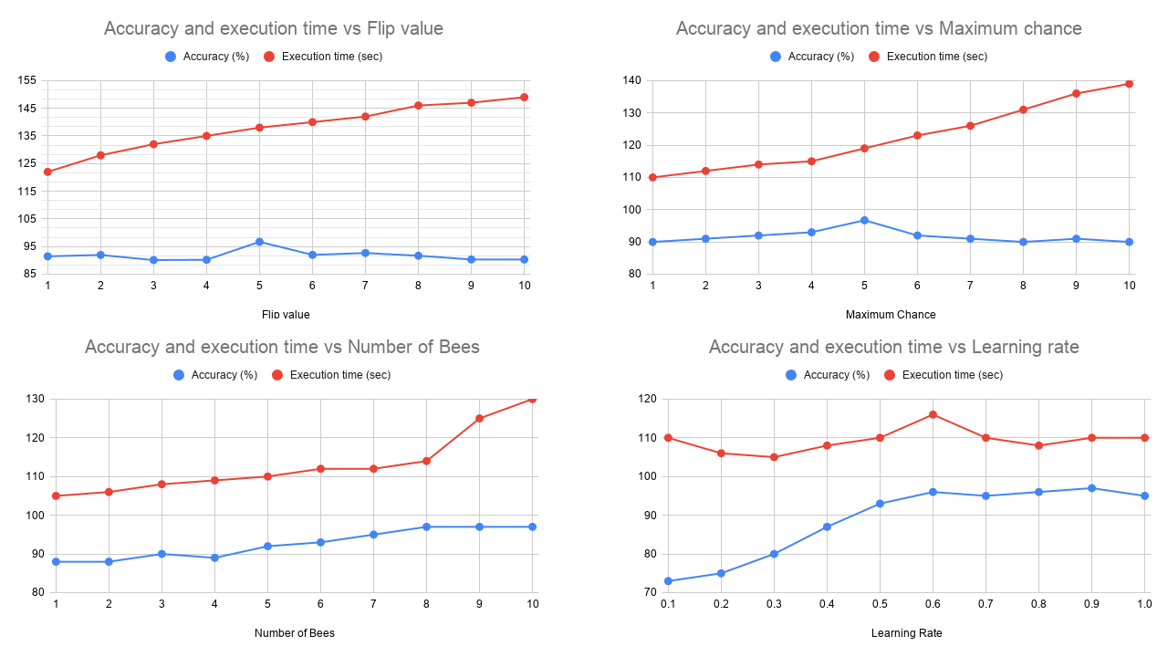
Figure 1: Analysis of classification accuracy and execution time vs. different parameters of the RSO algorithm

Parameter tuning has a pivotal role in the superior performance of any optimization algorithm. Hence, we have experimented with different parameters of the BSO and Residual Learning algorithm. To select the optimal set of parameters, the primary motive was to improve the classification accuracy as well as reducing the execution time. The optimal parameter setting for the algorithm was set experimentally by making a suitable compromise between these two conditions. Figure 1 shows the experimental results with different parameter tuning of the RSO algorithm using $Ionosphere$ dataset. Different BSO parameters like $Flip$, $MaxIter$, $ChanceMax$, $NumBees$, $LsIter$ were varied with integral differences from 1 to 10 wheres different RL parameters like $lr$, $\alpha$, $\beta$ are varied within the interval from 0 to 1 with an difference of 0.1, shown in Table II.

TABLE II: Optimal parameter setting for the RSO algorithm

Algorithm	Parameters	Optimal value
	Flip	5
	ChanceMax	5
	MaxIter	10
	NumBees	8
BSO	LsIter	10
	lr	0.9
	$\alpha$	0.2
RL	$\beta$	0.1

TABLE III: Comparison of the proposed RSO method with BSO method for feature selection along with classification performance without any feature selection. The highlighted results signify the best classification accuracy for the given setting.

	Without OA				Proposed Method						BSO
Dataset	Accuracy	Precision	Recall	F1 Score	Accuracy(%)	Precision	Recall	F1 Score	Number of feature	Time(sec)	Accuracy(%)	Precision	Recall	F1 Score	Number of feature	Time(sec)
Abalone	19.76	17.26	17.27	16.41	21.93	18	18.88	18.32	7	134	20.33	13.64	13.78	13.44	8	129
Australian	63.78	62.5	61.35	61.7	86.96	86.76	86.37	86.54	5	127	59.42	59.21	59.29	59.20	7	132
Biodegrade	81.04	79.32	79.19	79.8	84.15	86.93	85.31	86.24	13	146	79.24	77.42	78.01	77.68	16	141
Breastcancer	60	58.22	57.77	57.8	97.14	97.67	96.55	97.02	4	121	95.71	96.93	93.75	95.08	4	120
Breastcancer Wisconcin	87.71	87.86	84.79	85.99	95.16	95.29	95.29	95.29	11	139	87.71	87.46	86.89	87.14	10	135
Chess	51.27	49.64	46.72	45.29	51.27	49.64	46.72	45.29	6	95	20.20	17.52	16.29	16.28	7	100
Diabetes	66.23	61.62	60.36	60.65	72.72	69.58	68.73	69.11	4	126	72.72	70.91	70.61	70.75	4	124
Glass	74.41	70.83	67.59	64.37	85	88.69	90.28	87.95	7	133	54.54	46.66	43.61	44.8	8	130
Heart-C	42.62	31.73	29.11	28.98	58.39	59.66	53.4	55.62	2	130	54.83	24.98	30	26.58	4	129
Hepaitits	60	58.92	60	58.33	78.67	75.96	72.33	74.25	7	135	53.33	50	50	49.76	6	138
Ionosphere	85.71	87.07	84.86	85.28	96.72	91.66	91.18	91.31	15	138	88.96	92	86.66	87.95	20	142
Iris	93.33	94.44	93.33	93.27	97.85	99.23	96.19	97.33	2	105	86.64	86.11	86.11	86.11	2	101
LSVT	46.15	54.17	54.17	46.15	75.38	74.67	77.81	76.5	213	172	53.84	54.76	55	53.57	224	169
LungCancer	75.64	83.33	75	73.33	98.53	97.5	96.91	97.08	20	157	50	25	50	33.33	21	158
Parkinson	85	81.45	81.88	79.02	93.5	86.3	85.79	85.96	12	135	95	90	96.8	92.83	16	136
Sonar	78.57	78.6	78.41	78.56	98.31	96.63	96.23	96.22	30	160	85.71	86.05	84.72	85.17	42	157
Thyroid	100	100	100	100	100	100	100	100	5	104	90.93	86.92	86.92	86.92	5	99
Wine	60.51	55.36	52.89	53.44	97.22	97.41	97.22	97.22	9	124	100	100	100	100	10	120
Zoo	95	77.77	83.33	80	100	95	96.67	96.67	11	122	100	100	100	100	11	125
WDBC	77.19	75	75.54	76.24	95.32	94.75	94.75	94.75	14	135	94.73	95.94	93.47	94.39	14	130
Congress	93.18	93.37	92.73	93	97.95	96.54	96.28	96.25	6	127	95.45	93.75	96.66	94.94	9	132
Vowel	98.89	98.94	98.79	98.89	100	100	100	100	9	126	98.90	99.16	99.16	99.13	9	126
MovementLibras	86.11	87.56	87.17	86.71	83.33	86.42	83.33	83.52	22	161	80.55	80.35	80.71	77.09	25	164
Liver	62.23	61.79	60.33	60.98	64.86	63.24	65.51	62.03	4	120	62.34	61.22	63.59	64.55	5	114
Spect	51.25	50.23	50.02	53.66	77.47	76.33	75.89	76.32	16	129	72.01	70.22	73.69	70.66	14	128

TABLE IV: Comparison of the proposed RSO method with different existing feature selection methods for feature selection along with classification performance without any feature selection. The highlighted results signify the best classification accuracy for the given setting.

	Proposed method				PSO				MVO				GWO				MFO				WOA				HHO
Dataset	Accuracy(%)	Precision	Recall	F1 Score	Accuracy(%)	Precision	Recall	F1 Score	Accuracy(%)	Precision	Recall	F1 Score	Accuracy(%)	Precision	Recall	F1 Score	Accuracy(%)	Precision	Recall	F1 Score	Accuracy(%)	Precision	Recall	F1 Score	Accuracy(%)	Precision	Recall	F1 Score
Abalone	21.93	18	18.88	18.32	20.81	15.20	15.69	15.05	21.77	12.3	12.89	12.48	19.37	10.95	11.48	11.07	21.77	12.37	12.89	12.48	21.77	12.37	12.89	12.48	21.77	12.37	12.89	12.48
Australian	86.96	86.76	86.37	86.54	79.71	79.78	80.09	79.67	86.95	86.78	86.96	86.85	59.42	58.83	58.70	58.71	60.86	60.79	60.90	60.73	49.27	63.43	53.65	40.88	86.95	87.32	86.37	86.67
Biodegrade	84.15	86.93	85.31	86.24	80.18	78.44	79.33	78.81	81.13	79.46	80.65	79.92	83.01	81.54	81.54	81.54	81.13	79.48	79.48	79.48	75.47	73.33	72.75	73.01	82.07	80.86	83.12	81.34
Breastcancer	97.14	97.67	96.55	97.02	92.85	93.53	90.57	91.81	92.85	93.53	90.57	91.81	95.71	96.93	93.75	95.08	95.71	96.93	93.75	95.08	94.28	94.60	92.66	93.52	92.85	93.53	90.57	91.81
Breastcancer Wisconcin	95.16	95.29	95.29	95.29	89.47	89.06	89.06	89.06	89.47	89.68	88.36	88.89	87.71	87.12	87.59	87.32	89.47	89.68	88.36	88.89	94.73	94.87	94.18	94.49	94.73	94.87	94.18	94.49
Chess	51.27	49.64	46.72	45.29	34.06	34.64	40.60	35.54	49.46	46.64	51.45	47.93	47.46	30.14	29.81	29.91	49.46	46.64	51.45	47.93	49.46	46.64	51.45	47.93	49.46	46.64	51.45	47.93
Diabetes	72.72	69.58	68.73	69.11	76.62	75.32	77.15	75.93	76.62	75.71	77.15	75.93	76.62	75.71	77.15	75.93	75.32	74.21	75.43	74.48	76.62	75.71	77.15	75.93	72.72	70.91	70.61	70.75
Glass	85	88.69	90.28	87.95	59.09	52.77	50.27	51.11	59.09	52	45.83	48.01	54.54	47.77	43.61	45.39	59.09	52	45.83	48.01	54.54	46.66	43.61	44.81	54.54	45	43.88	44.41
Heart-C	58.39	59.66	53.4	55.62	32.25	16.85	16.66	16.25	51.61	24.28	20.66	21.09	45.16	15.55	15.55	15.55	51.61	28.88	31.77	26.82	51.61	21.64	23.33	22.14	48.38	35	34	33.56
Hepaitits	78.67	75.96	72.33	74.25	60	60.71	61.11	59.82	80	80	77.77	78.46	60	58.33	58.33	58.33	66.66	69.44	69.44	66.66	46.66	47.32	47.22	46.42	46.66	44.44	44.44	44.44
Ionosphere	96.72	91.66	91.18	91.31	77.77	86.20	73.33	73.81	77.77	86.20	73.33	73.81	75	79.46	70.95	71.25	77.77	86.20	73.33	73.81	77.78	86.20	73.33	73.81	75	85	70	69.74
Iris	97.85	99.23	96.19	97.33	100	100	100	100	100	100	100	100	100	100	100	100	100	100	100	100	100	100	100	100	100	100	100	100
LSVT	75.38	74.67	77.81	76.5	69.23	70.23	71.25	69.04	69.23	70.23	71.25	69.04	69.23	70.23	71.25	69.04	61.53	60.71	61.25	60.60	69.23	70.23	71.25	69.04	61.53	60.71	61.25	60.60
LungCancer	98.53	97.5	96.91	97.08	50	50	50	50	75	83.33	75	73.33	50	50	50	50	50	25	50	33.33	50	50	50	50	50	25	50	33.33
Parkinson	93.5	86.3	85.79	85.96	75	67.58	75	68.6	95	90	96.87	92.83	95	90	96.87	92.83	95	90	96.87	92.83	95	90	96.87	92.83	95	90	96.87	92.83
Sonar	98.31	96.63	96.23	96.22	76.19	78.33	73.61	74.07	66.66	66.66	63.88	63.70	100	100	100	100	90.47	90.27	90.27	90.27	76.19	78.33	73.61	74.07	71.42	74.37	68.05	67.85
Thyroid	100	100	100	100	90.90	86.92	86.92	86.92	100	100	100	100	100	100	100	100	100	100	100	100	100	100	100	100	100	100	100	100
Wine	97.22	97.41	97.22	97.22	66.66	62.5	60.71	61.32	94.44	95.83	95.23	95.21	100	100	100	100	94.44	93.33	95.23	93.73	100	100	100	100	100	100	100	100
Zoo	100	95	96.67	96.67	100	100	100	100	90.90	66.66	66.66	66.66	90.90	66.66	66.66	66.66	100	100	100	100	90.90	66.66	66.66	66.66	90.90	66.66	66.66	66.66
WDBC	95.32	94.75	94.75	94.75	87.71	89.52	85.48	86.66	87.71	87.46	86.89	87.14	78.94	78.94	76.72	77.38	89.47	89.68	88.36	88.89	84.21	83.76	83.24	83.47	91.22	92.09	89.83	90.66
Congress	97.95	96.54	96.28	96.25	90.90	88.83	91.42	89.88	90.90	88.88	93.33	90.17	95.45	93.75	96.66	94.94	97.72	96.66	98.33	97.42	97.72	96.66	98.33	97.42	90.90	88.88	93.33	90.17
Vowel	100	100	100	100	97.80	95.83	98.05	96.54	97.80	95.83	98.05	96.54	96.70	97.46	97.08	97.06	97.80	98.16	97.91	97.93	97.80	98.16	97.91	97.93	97.80	95.83	98.05	96.54
MovementLibras	83.33	86.42	83.33	83.52	80.55	80.35	80.71	77.09	83.33	81.30	84.28	79.99	83.33	82.14	82.5	79.47	83.33	81.66	84.28	79.86	80.55	81.76	80.71	77.73	77.77	80.65	78.33	76.16
Liver	64.86	63.24	65.51	62.03	61.25	60.94	61.27	61.11	62.66	62.47	63.08	62.69	63.52	62.63	63.02	62.94	62.66	62.47	63.08	62.69	60.78	61.29	60.36	63.52	62.63	63.02	62.94	62.66
Spect	77.47	76.33	75.89	76.32	75.88	76.36	76.55	76.48	75.88	76.36	76.55	76.48	75.88	76.36	76.55	76.48	76.15	75.89	76.32	76.06	75	75	75	75	75.88	76.36	76.55	76.48

III-C Performance evaluation

The performance of the proposed method was evaluated on 25 standard datasets where we have selected optimal feature subset using RSO followed by classification using KNN classifier. The classification performance was evaluated using the evaluation metrics given by Equation 5-8.

$$Accuracy=\frac{TP+TN}{TP+TN+FP+FN}$$ (5)

$$Precision=\frac{TP}{TP+FP}$$ (6)

$$Recall=\frac{TP}{TP+FN}$$ (7)

$$F1score=\frac{2}{\frac{1}{Precision}+\frac{1}{Recall}}$$ (8)

where $TP$ = True Positive, $FP$ = False Positive, $TN$ = True Negative, and $FN$ = False Negative.

III-D Comparison with existing methods

We have evaluated the performance of the proposed RSO method with different existing optimization algorithms. Table III shows the comparison of the experimental results in terms of accuracy, precision, recall, F1 score, execution time, and the number of selected features, obtained from our proposed method with the same obtained from the BSO algorithm.It is evident from the table that our proposed RSO method outperforms the BSO algorithm in 22 out of the 25 cases in terms of classification accuracy, by using a significantly smaller subset of feature data and thereby reducing the execution time.

We have also compared the obtained results with several feature selection algorithms like Particle Swarm Optimization (PSO) [2], Grey Wolf Optimization (GWO) [3], Genetic Algorithm (GA) [4], Harris Hawk Optimization (HHO) [29], Multi-Verse Optimization (MVO) [30], Moth Flame Optimization [31], Whale Optimization Algorithm (WOA) [32] as shown in Table IV. The proposed method outperformed all the methods compared in this paper in 19 out of 25 cases in terms of fitness of selected features, which is reflected in classification accuracy. However, our model performed inferior in the case of $Wine$ dataset with the best classification accuracy of 97.22% whereas most of the other methods were able to produce a superior feature subset, resulting in a classification accuracy of 100%. In the case of $Diabetes$ dataset, PSO, MVO, WOA and GWO performed the best with a classification accuracy of 76.62% as compared to 72.72% from the proposed RSO method. The MVO method performed the best in $Hepatitis$ dataset as compared to 78.67% from our proposed method. For $Iris$ dataset, all the methods produced a classification accuracy of 100% whereas the RSO method produced a result of 97.85%. MVO, MFO, WOA, and HHO produced similar results to the BSO method in $Parkinson$ dataset with a classification accuracy of 95% as compared to 93.5% of our proposed method. In the case of $Sonar$ data, the GWO performs the best with a classification accuracy of 100% as compared to 98.31% from RSO. Our proposed method performs the best in all other datasets as shown in Table IV.

IV Conclusion and future work

In this paper, we propose a new hybrid wrapper-based feature selection algorithm named RSO, which integrates the Residual Learning algorithm with the metaheuristic BSO algorithm. Experimental results show that our proposed method outperforms the BSO as well as the existing and popularly known metaheuristic optimization algorithms in feature selection task in terms of accuracy by selecting comparatively fewer optimal features. In future, we plan to extend our research by experimenting and observing the performance of different hybrid optimization algorithms. We also plan to observe the performance of RSO on deep features, to study the impact of RL in the performance of feature selection algorithms.

References

- [1] A. L. Blum and P. Langley, “Selection of relevant features and examples in machine learning,” Artificial intelligence, vol. 97, no. 1-2, pp. 245–271, 1997.
- [2] R. Eberhart and J. Kennedy, “A new optimizer using particle swarm theory,” in MHS’95. Proceedings of the Sixth International Symposium on Micro Machine and Human Science. Ieee, 1995, pp. 39–43.
- [3] S. Mirjalili, S. M. Mirjalili, and A. Lewis, “Grey wolf optimizer,” Advances in engineering software, vol. 69, pp. 46–61, 2014.
- [4] J. R. Schott, “Fault tolerant design using single and multicriteria genetic algorithm optimization,” Ph.D. dissertation, Massachusetts Institute of Technology, 1995.
- [5] D. Karaboga, “An idea based on honey bee swarm for numerical optimization,” Citeseer, Tech. Rep., 2005.
- [6] A. Bommert, X. Sun, B. Bischl, J. Rahnenführer, and M. Lang, “Benchmark for filter methods for feature selection in high-dimensional classification data,” Computational Statistics & Data Analysis, vol. 143, p. 106839, 2020.
- [7] R. J. S. Raj, S. J. Shobana, I. V. Pustokhina, D. A. Pustokhin, D. Gupta, and K. Shankar, “Optimal feature selection-based medical image classification using deep learning model in internet of medical things,” IEEE Access, vol. 8, pp. 58 006–58 017, 2020.
- [8] P. Hu, J.-S. Pan, and S.-C. Chu, “Improved binary grey wolf optimizer and its application for feature selection,” Knowledge-Based Systems, vol. 195, p. 105746, 2020.
- [9] X. Zhang, M. Fan, D. Wang, P. Zhou, and D. Tao, “Top-k feature selection framework using robust 0-1 integer programming,” IEEE Transactions on Neural Networks and Learning Systems, 2020.
- [10] L. Ke, Z. Feng, and Z. Ren, “An efficient ant colony optimization approach to attribute reduction in rough set theory,” Pattern Recognition Letters, vol. 29, no. 9, pp. 1351–1357, 2008.
- [11] O. Engin and A. Güçlü, “A new hybrid ant colony optimization algorithm for solving the no-wait flow shop scheduling problems,” Applied Soft Computing, vol. 72, pp. 166–176, 2018.
- [12] M. Amoozegar and B. Minaei-Bidgoli, “Optimizing multi-objective pso based feature selection method using a feature elitism mechanism,” Expert Systems with Applications, vol. 113, pp. 499–514, 2018.
- [13] Y. Zhang, D.-w. Gong, X.-y. Sun, and Y.-n. Guo, “A pso-based multi-objective multi-label feature selection method in classification,” Scientific reports, vol. 7, no. 1, pp. 1–12, 2017.
- [14] C. Yan, J. Ma, H. Luo, and A. Patel, “Hybrid binary coral reefs optimization algorithm with simulated annealing for feature selection in high-dimensional biomedical datasets,” Chemometrics and Intelligent Laboratory Systems, vol. 184, pp. 102–111, 2019.
- [15] M. M. Mafarja and S. Mirjalili, “Hybrid whale optimization algorithm with simulated annealing for feature selection,” Neurocomputing, vol. 260, pp. 302–312, 2017.
- [16] M. M. Kabir, M. Shahjahan, and K. Murase, “A new hybrid ant colony optimization algorithm for feature selection,” Expert Systems with Applications, vol. 39, no. 3, pp. 3747–3763, 2012.
- [17] S. Chattopadhyay, A. Dey, and H. Basak, “Optimizing speech emotion recognition using manta-ray based feature selection,” arXiv preprint arXiv:2009.08909, 2020.
- [18] J. Meshkati and F. Safi-Esfahani, “Energy-aware resource utilization based on particle swarm optimization and artificial bee colony algorithms in cloud computing,” The Journal of Supercomputing, vol. 75, no. 5, pp. 2455–2496, 2019.
- [19] Y. Djenouri, Z. Habbas, D. Djenouri, and P. Fournier-Viger, “Bee swarm optimization for solving the maxsat problem using prior knowledge,” Soft Computing, vol. 23, no. 9, pp. 3095–3112, 2019.
- [20] Y. Djenouri, A. Belhadi, and R. Belkebir, “Bees swarm optimization guided by data mining techniques for document information retrieval,” Expert Systems with Applications, vol. 94, pp. 126–136, 2018.
- [21] Y. Djenouri, D. Djenouri, A. Belhadi, P. Fournier-Viger, J. C.-W. Lin, and A. Bendjoudi, “Exploiting gpu parallelism in improving bees swarm optimization for mining big transactional databases,” Information Sciences, vol. 496, pp. 326–342, 2019.
- [22] L. Gao, M. Ye, and C. Wu, “Cancer classification based on support vector machine optimized by particle swarm optimization and artificial bee colony,” Molecules, vol. 22, no. 12, p. 2086, 2017.
- [23] H. Basak, R. Kundu, S. Chakraborty, and N. Das, “Cervical cytology classification using pca & gwo enhanced deep features selection,” arXiv preprint arXiv:2106.04919, 2021.
- [24] D. Teodorovic, P. Lucic, G. Markovic, and M. Dell’Orco, “Bee colony optimization: principles and applications,” in 2006 8th Seminar on Neural Network Applications in Electrical Engineering. IEEE, 2006, pp. 151–156.
- [25] L. P. Kaelbling, M. L. Littman, and A. W. Moore, “Reinforcement learning: A survey,” Journal of artificial intelligence research, vol. 4, pp. 237–285, 1996.
- [26] N. Metropolis and S. Ulam, “The monte carlo method,” Journal of the American statistical association, vol. 44, no. 247, pp. 335–341, 1949.
- [27] H. Song, C.-C. Liu, J. Lawarrée, and R. W. Dahlgren, “Optimal electricity supply bidding by markov decision process,” IEEE transactions on power systems, vol. 15, no. 2, pp. 618–624, 2000.
- [28] G. Tesauro, “Temporal difference learning and td-gammon,” Communications of the ACM, vol. 38, no. 3, pp. 58–68, 1995.
- [29] A. A. Heidari, S. Mirjalili, H. Faris, I. Aljarah, M. Mafarja, and H. Chen, “Harris hawks optimization: Algorithm and applications,” Future generation computer systems, vol. 97, pp. 849–872, 2019.
- [30] S. Mirjalili, S. M. Mirjalili, and A. Hatamlou, “Multi-verse optimizer: a nature-inspired algorithm for global optimization,” Neural Computing and Applications, vol. 27, no. 2, pp. 495–513, 2016.
- [31] S. Mirjalili, “Moth-flame optimization algorithm: A novel nature-inspired heuristic paradigm,” Knowledge-based systems, vol. 89, pp. 228–249, 2015.
- [32] S. Mirjalili and A. Lewis, “The whale optimization algorithm,” Advances in engineering software, vol. 95, pp. 51–67, 2016.