Spin and velocity correlations in a confined two-dimensional fluid of disk-shaped active rotors

Abstract

We study the velocity autocorrelations in an experimental configuration of confined two-dimensional active rotors (disks). We report persistent small scale oscillations in both rotational and translational velocity autocorrelations, with their characteristic frequency increasing as rotational activity increases. While these small oscillations are qualitatively similar in all experiments, we found that, at strong particle rotational activity, the large scale particle spin fluctuations tend to vanish, with the small oscillations around zero persisting in this case, and spins remain predominantly and strongly anti-correlated at longer times. For weaker rotational activity, however, spin fluctuations become increasingly larger and angular velocities remain de-correlated at longer times. We discuss in detail how the autocorrelation oscillations are related to the rotational activity and why this feature is arguably should generically signal the emergence of chirality in the dynamics of a particulate system.

I Introduction

Active matter comprises units that convert either internal or external energy into motion with a systematically directed component Dombrowski et al. (2004); Marchetti et al. (2013); Zhang et al. (2010); Petroff, Wu, and Libchaber (2015); Xu et al. (2022). This directional, active, motion induces a parity and time inversion symmetry break. Because of this, active matter frequently exhibits an intrinsic and rich collective phenomenology, not present in systems of pasive particles Bowick et al. (2022). For instance, the dynamics of these systems displays spontaneous self-organization Nguyen et al. (2014), peculiar phase separation (induced by active motion, and for this reason known as motility induced phase separation, or MIPS) Cates and Tailleur (2015); Caporusso et al. (2020); Großmann, Aranson, and Peruani (2020), flocking and swarming Liao, Hall, and Klapp (2020); Gupta et al. (2020); Zhang et al. (2010); Bricard et al. (2015), and flow chirality (flows that develop patterns with chiral asymmetry) Zhang, Sokolov, and Snezhko (2020); López-Castaño et al. (2022); Mokhtari, Aspelmeier, and Zippelius (2017); Farhadi et al. (2018); Workamp et al. (2018). In the case of chiral flows, its origin lies most frequently in the geometrical chirality of active particles that compose the system Tsai et al. (2005).

A number of fundamental aspects of the dynamics of active rotors presents very distinctive features when compared to other equilibrium and non-equilibrium fluids. For instance, transport phenomena display in chiral fluids a much more complex behavior, due to the emergence of antisymmetric components in the fluxes (of mass, momentum and energy) Banerjee et al. (2017); Hargus, Epstein, and Mandadapu (2021); Han et al. (2021). As a consequence, the constitutive relations for these antisymmetric components of the fluxes involve the definition of new set of transport coefficients with special properties. As an example, fluid flow and diffusion are controlled by the so-called odd viscosity Avron (1998); Banerjee et al. (2017); Han et al. (2020) and odd diffusion Hargus, Epstein, and Mandadapu (2021); Vega Reyes, López-Castaño, and Rodríguez-Rivas (2022) coefficients, both of these coefficients being specific of chiral fluids. In the case of a fluid of active rotors, the chirality of the fluid is due to particle systematic rotation (which, on the other hand, may have different origins). Thus, it is in this systematic rotation where we may identify the origin of the peculiar transport properties of fluids of active rotors. Due to this, the statistical properties of particle rotations can be identified as an essential feature for this kind of chiral fluids and thus, one can reasonably expect the angular velocity statistical correlations to be one of the essential factors in the dynamics of the chiral fluid.

However, there is still little to no bibliography (to our knowledge) on the study of statistical correlations in active rotors, specially with regard to angular velocities (for two very recent studies on translational velocity correlations, in chiral fluids, see Zhang, Sokolov, and Snezhko (2020); Debets, Löwen, and Janssen (2023)). In summary, the understanding of these correlations in chiral flows is still very preliminary. In fact, results in a previous work suggest López-Castaño et al. (2022) that the structure of statistical correlations is an essential factor determining the fluid flow properties in a system of active rotors.

Thus, the motivation of the present work is to perform a detailed and specific analysis of the statistical correlations of angular velocities in a two-dimensional fluid of active rotors. For this objective, we study an experimental system composed of macroscopic and flat disk-shaped rotors. These disks are provided with 14 equal size tilted blades (see Figure 2 a). An air upflow passes past the disks, which induces a Brownian-like translational stochastic motion Ojha et al. (2004) and, at the same time, creates a biased particle rotation due to the presence of the tilted blades.

For our purpose, we set-up an air table that aids fluidization in a system of 3D printed disks. An ad-hoc fan provides stable continuous current, that is on purpose homogenized before impinging the particles from below. As a consequence, particles continuously undergo a systematic torque $\tau_{0}$ which inforces them to set back a particular value of average spin after momentum-transfer events (which in this case are either particle-particle or particle-boundary collisions). This yields a systematic rotational activity to the rotors, as we will explain. As a consequence, the system features peculiar statistical properties of the translational and angular velocities. In particular, we show there are two regimes of the angular velocity correlations (at strong and weak fluidization) for which spin autocorrelations are stronger and weaker respectively. However, translational velocities tend to decorrelate at intermediate fluidization whereas autocorrelations are strong at both weak and strong fluidization. We also report the existence of persistent oscillations in the autocorrelation function of particle spin. We describe in more detail in the remainder of this work the features of statistical velocity correlations in our system.

This work is organized as follows. In section II we provide details on the experimental configuration used for this work, along with a description of the algorithm we wrote for particle angle tracking which, as we will explain, achieves a very high time accuracy. Additional details related to this section, including a detailed analysis of experimental errors, can be found in the Appendix. In Section III we show the data obtained from experiments, and analyze the results focusing on the translational and angular velocity correlations. Finally, in Section IV , we discuss and summarize the results.

II Experimental set-up

II.1 Description

The fluid consists of a set of $N$ identical disk-shaped particles. Their diameter is $\sigma=72.5\pm 0.1~{}\mathrm{mm}$ and their thickness is $h=6.0\pm 0.1~{}\mathrm{mm}$. Thus, they can be considered nearly flat (i.e., two-dimensional). Their mass is $m_{p}=7.76\pm 0.01~{}\mathrm{g}$, and they were produced by means of additive 3D printing (material is polylactic acid). The disks incorporate a set of $N_{b}=14$ equally-spaced identical blades (reproducible 3D models, in .stl format, are available upon request). We measured the mass and size distribution of our set of disks, in order to control the reproducibility of the printing process. The moment of inertia of the particles, $I$ is considered to be approximately that of a homogeneous disk. The particle design is rendered in Fig. 1(a).

The disks are placed over a perforated square metallic grid ($100\times 100~{}\mathrm{cm}$) and are enclosed inside a circular wall. This wall is centered in the square grid, with height $40~{}\mathrm{mm}$ and diameter $L=72.5\pm 0.1~{}\mathrm{cm}\simeq 10\,\sigma$. For convenience, we define also the system radius $R=L/2\simeq 5\,\sigma$. It is convenient to define also the packing fraction as $\phi=N(\sigma/L)^{2}\simeq N/100$. We have performed experiments for three different packing fractions $\phi=~{}0.25,~{}0.45$ and $0.55$, which correspond here to $N=25,45$ and $55$ particles, respectively.

An air flow is produced by means of a high precision air fan (SODECA HCT-71-6T model), which can move air volumes of up to $1.51\times 10^{4}~{}\mathrm{m^{3}/h}$. This fan is disposed so that initially releases the air horizontally to a horizontal channel. This flow is afterwards redirected to the vertical by means of a second channel, so that the air current impinges the particles from below. An intermediate foam is placed within the vertical channel, with the aim of improving the upflow homogeneity Ojha et al. (2004). Figure  1(b) shows a sketch of the experimental set-up.

Fan power is adjusted so that all particles horizontally levitate just over the grid, thus avoiding friction. The grid has been carefully levelled horizontally so as to avoid gravity effects. The upflow intensity working range is delimited here by the minimum fan power necessary for the particles to levitate and the maximum value before they start to undergo vertical displacements (thus loosing stable horizontal alignment). In addition, the upflow past the blades produces a continuous particle rotation. Therefore, in our experiments, particle movement (rotation and translation) is limited to the grid plane at all times, and is essentially two-dimensional. We checked that deviations of the disk surface from the horizontal are less than 1% during experiments. Moreover, according to our measurements from a digital anemometer, the air current intensity at the level of the grid is constant in time and is spatially homogeneous, with deviations from the spatially averaged value of less $5\%$.

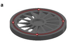
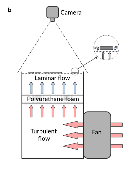
Figure 1: (a) Renderization of the 3D printed disk, with its 14 blades. (b) Representation of the experimental set-up.

Turbulent vortexes are generated out of the von Karmann streets that are produced after a fluid flow past an obstacle Dyke (1982); Taneda (1978) (in this case, the disks). Due to the present geometrical configuration, the typical length scale of these vortexes in our system is of the order of the particle size Ojha et al. (2004); López-Castaño et al. (2021). This effectively induces Brownian-like movement in the particles, which in this way acquire a fluctuating component in their translational velocities. Thus, a collisional regime is produced in the system, that so becomes fluidized Kanatani (1979). Moreover, collisions also induce a fluctuating component in particle spins, since there is angular momentum transfer due to friction effects upon collision Nowak et al. (1998).

We performed a sufficiently complete set of experiments at different densities and fan power (which results in different degrees of fluidization). Experiments were recorded for $27~{}\mathrm{s}\gg\tau$ ($\tau$ being the typical time between collisions), for this set of experiments implies the system is aged on average up to $10^{3}$ collisions per particle, in order of magnitude; i.e., steady state conditions are achieved in all experiments during long time intervals (systems of macroscopic particles typically achieve steady state after less than 10 collisions per particle Montanero and Santos (2000)).

For experiment recording, we used high-speed camera (Phantom VEO-410L) at a resolution of $1280\times 800$ pixels and a frame rate of 900 fps. At our working image resolution and camera position, the pixel width is equivalent to $1~{}\mathrm{px}=0.9295~{}\mathrm{mm}\simeq 10^{-3}\sigma$, which means that we can potentially measure particle position to a high degree of accuracy. See the Appendix A.2 for more information on the error in the experimental measurements.

Translational velocity and angular velocity (or spin) are denoted as $\mathbf{v}$ and $\mathbf{w}=w_{z}\mathbf{\hat{e}}_{z}$ respectively. The unit vector $\mathbf{\hat{e}}_{z}$ is perpendicular to the metallic grid and pointing upwards. We denote the time and spatial averages of particle velocity and spin as $\langle\mathbf{v}\rangle,\langle w\rangle$, respectively. We also define the ensemble averages

$$T_{t}(r)=(m/2)\langle(\mathbf{v}-\langle\mathbf{v}\rangle)^{2}\rangle,$$ (1)

$${T_{r}^{*}}(r)=(I/2)\langle(\mathbf{w}-\langle\mathbf{w}\rangle)^{2}\rangle,\quad{T_{r}}(r)=(I/2)\langle w^{2}\rangle,$$ (2)

which denote fluctuating translational kinetic energy ($T_{t}(r)$), fluctuating rotational kinetic energy ($T^{*}_{r}(r)$) and rotational kinetic energy ($T_{r}(r)$). Due to the specific geometry in the system, the steady states only depend on the spatial coordinate $r$ (distance to system center). We also define the corresponding spatially averaged (over the complete system) magnitudes: $\overline{T_{t}},\overline{T_{r}},\overline{T_{r}^{*}}$. $\overline{T_{r}}$ can be considered as the parameter that quantifies rotational activity; i.e., systematic rotation, see definition of $T_{r}$ in (1).

II.2 Particle position and angle tracking

Since our aim is to measure spin and velocity correlations, we first need to track particle positions and angular displacements. For this purpose, we specifically wrote for this work a particle position/angle tracking algorithm. For the translational part, our algorithm adapts several functions from the TrackPy Allan et al. (2019) and the OpenCV libraries Bradski (2000). (Trackpy is an adaptation to Python language of the particle-tracking algorithm originally developed by Crocker and Grier Crocker and Grier (1996))

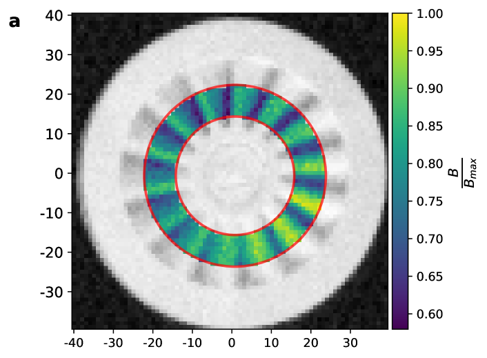
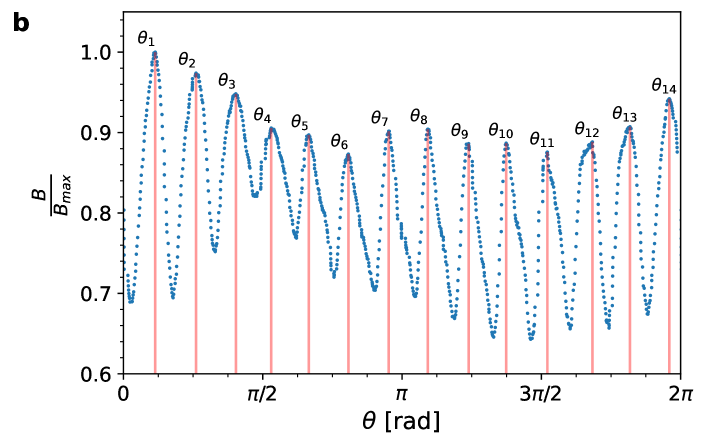
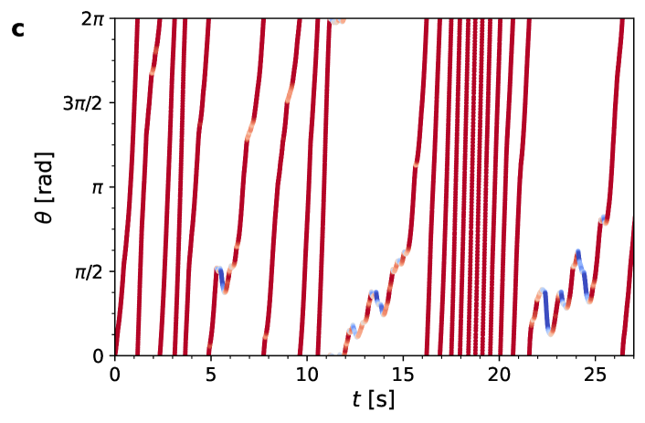
Figure 2: (a) Image of a single disk, axis units are in pixels. The hightligthed area is the one used to calculate rotational spin velocity (see methods). (b) Distribution of normalized pixel values (y-axis), vs. angle in a frame. (c) Particle spin vs. time for a representative particle, in an experiment with $N=55$ particles and $\overline{T_{t}}=0.91~{}m_{p}\sigma^{2}/\mathrm{s}^{-2}$.

With respect to angle tracking, and in order to avoid periodicity effects, the camera speed is adjusted so that the typical angular displacement between consecutive frames is not larger than half the angle between adjacent blades (i.e., $\theta(t+dt)-\theta(t)<\pi/14$). In our experimental configuration, this leads us to a minimum working frame rate of approximately $250~{}\mathrm{fps}$ (fps stands for frames per second). Therefore, for tracking angular displacements, we have recorded all experiments movies at $900$ fps (thus, we do not miss the large angular displacement tails of the corresponding distribution function). This procedure will allow us, as we will see, to achieve a high accuracy and capture finer scale details of the rotational dynamics.

The angle tracking algorithm works in the following steps:

1. In each frame, at a given time $t$, and for each particle, we obtain the brightness profile $B_{i}(\theta,t)$ out of 2D spatial average of pixel value over a centered annulus (where $i=1\dots N$ is the particle number and $\theta$ is the polar angle with respect to an arbitrary reference axis). Within this annulus, each $B_{i}(\theta,t)$ value is obtained from averaging pixel value, for $\theta$-constant pixels, from the inner to outer radii values of the annulus. In addition, each $B_{i}(\theta,t)$ is smoothed out by means of a Gaussian filter, for optimal accuracy. Examples of the centered annulus for brightness averaging and the obtained brightness profile $B_{i}(\theta,t)$ can be found in 2(a) and (b) respectively.

2. After this, and for each $B_{i}(\theta,t)$, we determine the set of $N_{b}$ maxima $\{\theta_{j}(t)\}$ ($j=1\dots N_{b}$ is the blade index). There are always $N_{b}$ maxima for each $B_{i}(\theta,t)$ profile since each maximum corresponds to the tallest part of a blade (because is closest to a homogeneous light source, from above). Thus, each maximum is identified as the angular position of one of the blades, for a given frame. This is illustrated in Fig. 2(b).

3. Finally, the profiles of consecutive frames are iteratively cross-correlated Press et al. (2007) for each particle, $B_{i}(\theta,t),\,B_{i}(\theta,t+dt)$. Specifically, cross-correlation is performed by using a fast Fourier transform method sci . From the cross correlation, each maximum in the set is physically identified in the next set of maxima $\{\theta_{j}(t+dt)\}$. In this way, we obtained linked $\theta_{j_{1}}(t)\to\theta_{j_{2}}(t+dt)$ and, therefore, the blades angular positions can be tracked throughout the entire movie. By applying differences between consecutive linked blade positions, we obtain instantaneous angular velocities.

The angular trajectory of a blade is represented in Fig. 2(c). First, notice that, since angle is periodic (between 0 and $2\pi~{}\mathrm{rad}$), tracks disappear and reappear in top and bottom limits of the figure panel. Also, here symbol colors indicate counter-clockwise (blue) and clockwise (red) particle spin (in this case, corresponds entirely to downwards or upwards slope, respectively). Point opacity is proportional to angular velocity $w$. A completely transparent point denotes for $w=0$; i.e., particle spin inversion. As we can see, most of the time particle spin is clockwise, since according to the design of the blades, they rotate clockwise under upflow. However, from time to time, spin reverses, which can be attributed to frequent particle collisions. This is further illustrated in the Appendix, in Fig. 8 (multimedia view).

From our discussion in the Appendix A.2, the maximum typical error from our experimental/particle-tracking methods are $\delta r\simeq 1.7\times 10^{-3}~{}\sigma$ for particle position and $\delta\theta\simeq 3.5\times 10^{-3}~{}\mathrm{rad}$ for particle angle. This is equivalent to about $0.01\%$ of particle diameter and $0.78\%$ of the angle between consecutive blades, which means that errors are here very narrow and our translational and angular velocity measurements very accurate.

III Results and Discussion

We performed a series of measurements, varying fan power at constant packing fraction. This process was repeated for a set of different values of packing fractions $\phi=~{}0.25,~{}0.45$ and $0.55$. Increasing air upflow intensity leads to higher average kinetic energy of the particles ($\overline{T_{t}}$) López-Castaño et al. (2022). In this way, we thoroughly analyzed the behavior of translational and rotational autocorrelations in the system, in a wide region of the relevant parameter space.

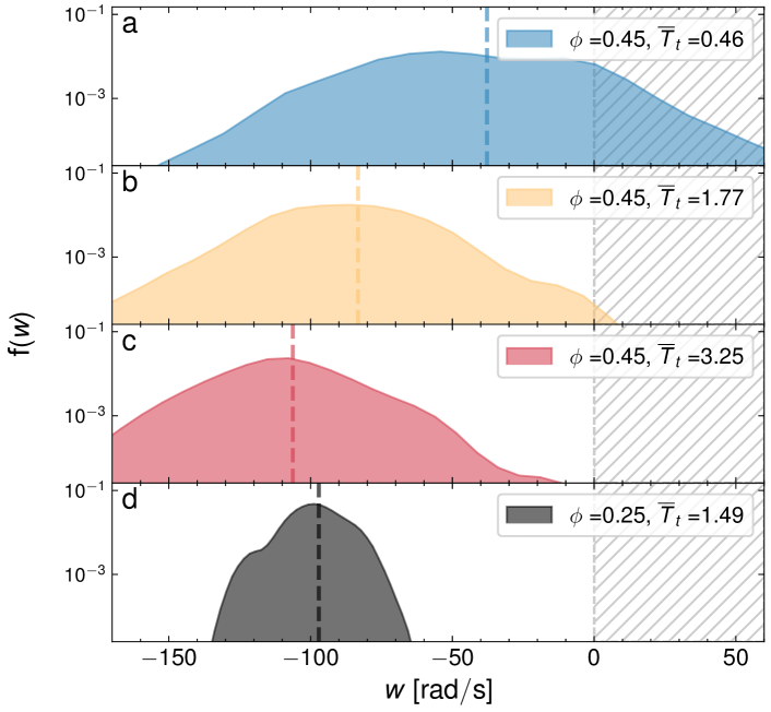
Figure 3: (a)-(c) Distribution function of particle angular velocities, $f(w)$, for 3 experiments with increasingly high $\overline{T_{t}}$, for constant packing fraction $\phi=0.45$. (d) $f(w)$ for $\phi=0.25$ (less dense than the previous cases), $\overline{T_{t}}=1.49~{}\sigma^{2}s^{-2}\mathrm{m_{p}}^{-1}$. For better visualization of the drift of $f(w)$ with $\overline{T_{t}}$ increasing, a common X-axis has been set for all four panels.

Since all movie experiments were recorded under steady state conditions, we can average over all instantaneous states, thus increasing the statistical accuracy of our analysis (we have nearly 25000 steady state snapshots).

We show in Fig. 3 the distribution function of particles angular velocities (or spin, $w$), $f(w)$. Particles tend to rotate clockwise by default ($w<0$), due to the particular tilt angle of their blades, and for this reason $w$ is predominantly negative. However, as it can be seen in certain cases, there is also a significant part of the distribution function under positive values of $w$ due to particle collisions. In any case, as we can see in Fig. 3, the vertical lines signal an average spin $\langle w\rangle$ that is always negative. Moreover, the region $f(w>0)\neq 0$ decreases as fan power is increased. This points out, in our opinion, the fact that collisions have a stronger influence in the dynamics at low $\overline{T_{t}}$ (i.e., at low fan power). Notice also that, as expected, when increasing higher upflow intensity (fan power), the distribution shifts towards faster ranges of (negative) particle spin and at the same time its width shrinks. As a result of both tendencies combined, absolute value of the average particle spin increases and, more interestingly, the fraction of particles with positive spin values significantly shrinks at intermediate fan power, finally disappearing at the largest values of $\overline{T_{t}}$ (or equivalenty, as we said, fan power). $\overline{T_{t}}$ is expressed in energy units: $m_{p}\sigma^{2}/\mathrm{s}^{-2}$). The existence of non-vanishing $f(w>0)$ would be related thus to emergent velocity correlations upon collision, which in this case would be mediated by frictional effects.

In Fig. 4, we represent $\overline{T_{r}},\overline{T_{r}^{*}}$, reduced with the value $\overline{T_{r}^{*}}(\phi=0.03)=\overline{T_{\mathrm{ref}}^{*}}=3.37~{}m_{p}\sigma^{2}/s^{2}$. As we can see, $\overline{T_{r}}$ increases for increasing $\overline{T_{t}}$. Thus, henceforth, recall that increasing $\overline{T_{t}}$ implies increasing $\overline{T_{r}}$ and vice versa. This is expected since the torque exerted on the disk blades, $\tau_{0}$, would logically be stronger for higher air current intensity. However, it can also be seen that the rate of growth for $\overline{T_{r}}$ also depends on particle density, since it tends to lower for higher particle density. This is consistent with the fact that inelastic cooling rate due to collisions increases with density Vega Reyes, Santos, and Kremer (2014). However, and very interestingly, the fluctuating rotational energy $\overline{T_{r}^{*}}$ behaves exactly in the opposite way. This clearly indicates that stronger torque $\tau_{0}$ (more intense particle activity) correlates more effectively particle spin and they tend more efficiently towards a fixed (and higher) value. This result is important since, as we will see, advances the existence of two differentiated regimes in the dynamics: a first regime at low fluidization where collisions decorrelate particles spins (high $\overline{T_{r}^{*}}$), and a second regime at high fluidization for which particle spins are highly correlated and particle activity predominates.

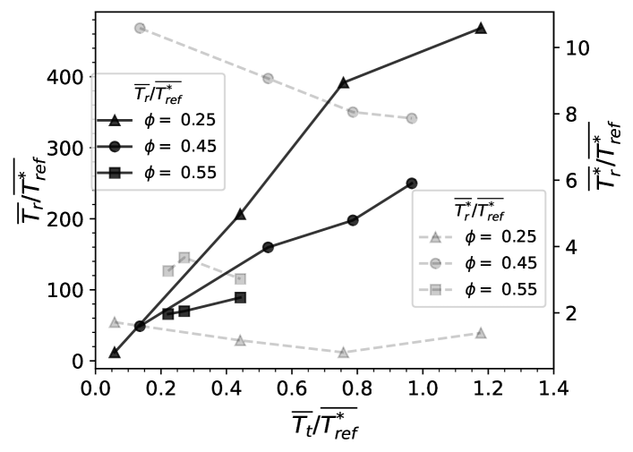
Figure 4: $\overline{T_{r}}$ (left Y-axis, black solid lines) and $\overline{T^{*}_{r}}$ (right Y-axis, grey dashed lines) vs. $\overline{T_{t}}$ for three representative values of packing fraction $\phi$ (legend). We use the value of $\overline{T_{r}^{*}}$ for the most dilute configuration we used for experiments (at packing fraction $\phi=0.03$), $\overline{T_{\mathrm{ref}}^{*}}$, as a reference value for dimensionalization of Y-axes.

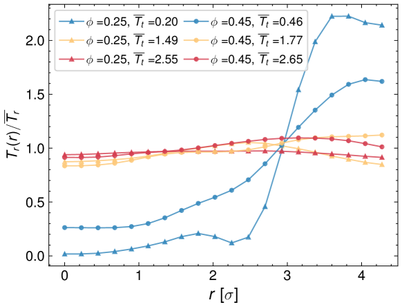
Figure 5: Radial profile of $T_{r}(r)/\overline{T_{r}}$ for two different packing fractions $\phi=0.25;~{}0.45$, (symbols ($\blacktriangle$) and ($\bullet$) respectively). For each packing fraction, three samples at different $\overline{T_{t}}$ are shown (blue, yellow and red symbols, respectively): $\overline{T_{t}}=0.20;1.49;2.55$ for $\phi=0.25$ and $\overline{T_{t}}=0.46;1.77;2.65$ for $\phi=0.45$. A step gradient is seen in the lowest thermalization cases, as further explained in the text.

In order to further investigate on the behavior of spin fluctuations and rotational kinetic energy, we represent in Fig. 5 the profiles of $T_{r}(r)/\overline{T_{r}}$. This is presented for a set of experiments at different constant values of $\phi,\overline{T_{t}}$. Blue curves stand for low $\overline{T_{t}}$ experiments whereas orange and red denote intermediate and high $\overline{T_{t}}$ respectively. Accordingly, experiments with $\phi=0.25$ are signaled with triangle symbols and experiments series with $\phi=0.45$ are denoted with circles. The results clearly show a transition from step function behavior at low $\overline{T_{t}}$ (blue curves) to a nearly flat behavior for highly fluidized states (higher $\overline{T_{t}}$) (orange/red curves). Furthermore, this transition appears consistently at low ($\phi=0.25$) and high densities (here we show $\phi=0.45$). This step-like behavior at low fluidization indicates that non-homogeneity of the average rotational energy is very large, with the spins in the inner part of the system rotating significantly slower (i.e., $T_{r}(r<R/2)/\overline{T_{r}}\to 0$), but with a steep increase at $r\simeq R/2$. On the contrary, at high and moderate fluidization, spin variations remain moderately small and the profiles are nearly homogeneous throughout the system ($T_{r}(r)/\overline{T_{r}}\simeq 1$). This enhances the idea that there are two clearly differentiated regimes with respect to particle spin correlations. The step-shaped form in $T_{r}/\overline{T_{r}}$ can be attributed to inelastic cooling Goldhirsch I (1993), which in the geometry of our system induces a higher concentration of particles in the center, thereby causing more energy dissipation at small $r$ and thus comparatively lower $T_{r}(r)$. The fact that this mechanism is less efficient at high $\overline{T_{t}}$ is arguably due to the strengthened underlying chiral flow pattern at higher $\overline{T_{t}}$, which can aid the heat flux inwards López-Castaño et al. (2022).

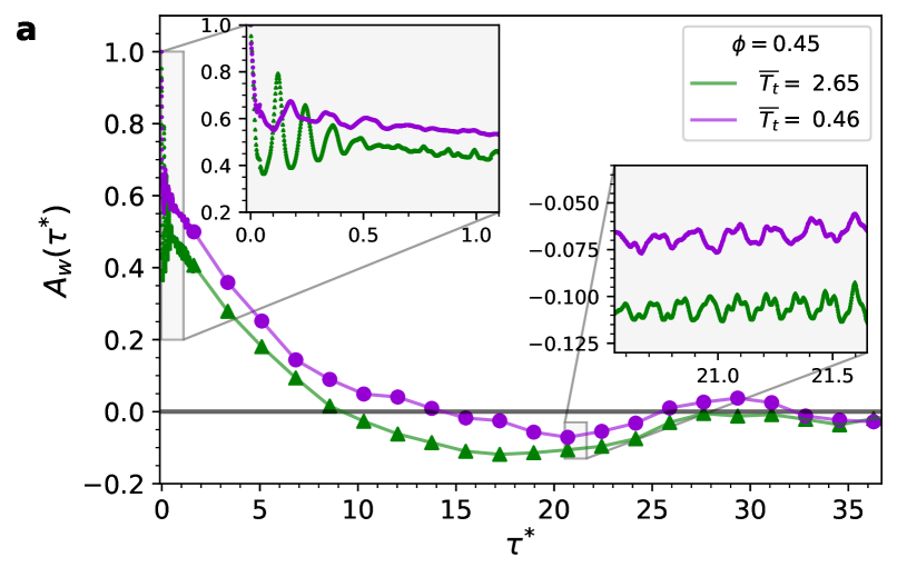
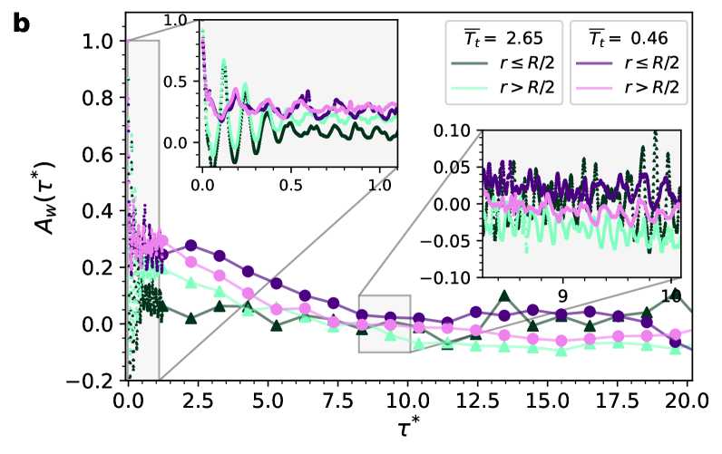
Figure 6: (a) Spin autocorrelation function, $A_{\bm{\mathbf{W}}}(\tau^{*})$. We compare two cases with the same density ($\phi=0.45$) but different translational kinetic energies ($\overline{T_{t}}$ in units of $m_{p}\sigma^{2}\mathrm{s}^{-2}$). Notice the small scale oscillations in left and right insets (at short and long delay times respectively). Their characteristic frequency is noticeably higher for higher rotational activity (equivalent to higher $\overline{T_{t}}$) (b) The same data sets as in the previous panels, split into two regions: $r<R/2$ and $r>R/2$. Again, insets zoom in for better visualization of small scale oscillations.

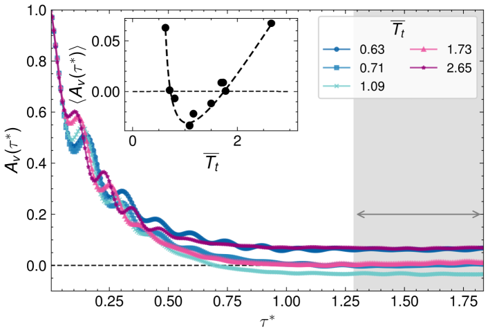
Figure 7: Velocity autocorrelation function $A_{\mathbf{v}}(\tau^{*})$ for a series of experiments with constant packing fraction ($\phi=0.45$) and increasing $\overline{T_{t}}$ (in units of $m_{p}\sigma^{2}\mathrm{s}^{-2}$). In the main plot we have represented the short time behavior, which fastly delivers a stationary plateau in all cases (signaled by the gray background). Notice the small scale oscillations, that have higher frequency for higher $\overline{T_{t}}$, and are rather similar to the ones in the $A_{\mathbf{W}}(\tau^{*})$ function, appear here as well. The inset represents the averaged values of the velocity autocorrelation function $A_{\mathbf{v}}(\tau^{*})$ (the average is performed over the stationary interval that is shaded in gray in the main panel). We added a dashed curve here, as a guide to the eye.

For this reason, and with the aim of providing more detail on the evolution of the autocorrelations Allen and Tildesley (2017) of the fluctuating spins $\mathbf{W}(t)=\mathbf{w}(t)-\langle\mathbf{w}\rangle$, we define the spin autocorrelation function as:

$$A_{\mathbf{W}}(\tau)=\frac{\langle\mathbf{W}(t)\cdot\mathbf{W}(t+\tau)\rangle}{\langle\mathbf{W}(t)\cdot\mathbf{W}(t)\rangle},$$ (3)

where again, $\langle\dots\rangle$ stands for averaging over all particles and steady states at arbitrary times $t$ and fixed.

Figure 6 shows the results we obtained for $A_{\mathbf{W}}(\tau^{*})$, for an experiment with $\phi=0.45$ and two different values of $\overline{T_{t}}$. Here, $\tau^{*}\equiv\tau/\tau_{\mathrm{ref}}$, with $\tau_{\mathrm{ref}}={(\overline{T_{\mathrm{ref}}^{*}}m_{p}^{-1}\sigma^{-2})}^{-1/2}$ is a reference time unit we used for in Figures 6, 7. We picked this specific value as time unit since it refers to the most dilute system in our set of experiments (we recall, $\overline{T_{\mathrm{ref}}^{*}}\equiv\overline{T_{r}^{*}}(\phi=0.03)$). In this way, we can refer results to a system where particles collisions are the least significant and then refer the increase of their influence for the rest of configurations. In the left panel, Fig. 6(a), we represent the global space average of $A_{\mathbf{W}}(\tau^{*})$ whereas Fig. 6(b) represents spatial averages inside the inner and outer annular halves of the system, so as to detect eventual differences in the correlations due to, for instance, boundary conditions. From results in Fig. 6(a), it is clear that our new measurement method captures in great detail the characteristic behavior of $A_{\mathbf{W}}(\tau^{*})$ Berne (1972); Lowe, Frenkel, and Masters (1995); Lokotosh, Malomuzh, and Shakum (2002) since we are able to detect short scale oscillations (which are shown in great detail in the inset).

It is very noticeable that the frequency of these tiny oscillations increases with increasing $\overline{T_{r}},\overline{T_{t}}$. Furthermore, these oscillations begin at very short times (of the order of the inverse average particle spin) and that they persist at longer times (although with a much smaller amplitude); i.e., they are present at all evolution times of the particle dynamics. Therefore, according to all of these observations, we can outline a plausible explanation by recalling also that particles undergo a rotational activity due to the systematic torque $\tau_{0}$ that the upflow yields. We think this would be the origin of these small oscillations (this in fact being also consistent with their persistence). In effect, each time a particle undergoes a spin fluctuation (and thus a slight decrease of $A_{\mathbf{W}}(\tau^{*})$), then it rapidly reacts by setting back to the value of average spin that $\tau_{0}$ will impose (slight increase of $A_{\mathbf{W}}(\tau^{*})$), and hence the oscillations. Since this torque increases for higher $\overline{T_{t}}$, then it is to be expected that the tendency of the particle to setting back the spin precollisional value (by default, closer to the average spin) is stronger as well as faster. Hence, the increase in the frequency of the oscillations of $A_{\mathbf{W}}(\tau^{*})$ for increasing $\overline{T_{t}}$. Furthermore, we have observed that the typical frequency of oscillations of spin autocorrelations is of the order of $10^{-2}~{}\mathrm{s}^{-1}$, which is analogous to the order of magnitude of the typical values of average particle spin López-Castaño et al. (2022) (we also recall again that, as Fig. 4 reveals, in our setup, $\overline{T_{r}}$ and hence average particle spin inherently increases with $\overline{T_{t}}$).

As we said, Fig. 6(b) represents a spatial analysis of the behavior of spin autocorrelations. In particular, we represent the same experiments at strong and weak fluidization that were shown in Fig. 6(a), but each split into two sets, each representing $A_{\mathbf{W}}(\tau^{*})$ averaged over only the outer ($r>R/2$) and only inner half ($r<R/2$) of the system. Experimental data shows here that spin autocorrelations are slightly more prominent in the outer part of the system at short times. At intermediate times, there is a crossover which renders autocorrelations slightly stronger in the inner part of the system. This crossover seems to be also more noticeable at higher fluidization (dark/light green data sets). However, differences between inner and outer halves of the system are not significant. In general, notice also that spins remain importantly anti-correlated at long times in the case of high $\overline{T_{t}}$ whereas for low $\overline{T_{t}}$ autocorrelations remain close to zero; i.e., spins tend to decorrelate at longer times only at low fluidization, which is reasonable because of the lower systematic torque $\tau_{0}$ on the particles at low $\overline{T_{t}}$. Significantly, smaller scale oscillations due to systematic torque still survive at all times in both inner and outer regions, even if $A_{\mathbf{W}}(\tau^{*})\to 0$ at longer times (since systematic torque $\tau_{0}$ is always present).

Finally, we have also studied the behavior of the conventional velocity autocorrelation function

$$A_{\mathbf{v}}(\tau)=\frac{\langle\mathbf{v}(t)\cdot\mathbf{v}(t+\tau)\rangle}{\langle\mathbf{v}(t)\cdot\mathbf{v}(t)\rangle}$$ (4)

Figure 7 shows the results for a series of experiments with increasing $\overline{T_{t}}$, at constant packing fraction $\phi=0.45$. As we can see, the decay to zero of the $A_{\mathbf{v}}(\tau^{*})$ curves is significantly faster if compared to that of $A_{\mathbf{W}}(\tau^{*})$ curves (Figure 6). In effect, this decay is typically observed within time intervals of less than $0.5~{}\mathrm{s}$, as compared to the $5~{}\mathrm{s}$ that spin autocorrelations take to fall to zero. This would be due to the fact that particle collisions are more effective in decorrelating translational velocities since spins tend to remain correlated upon collision due to the presence of rotational activity (i.e., the systematic torque $\tau_{0}$).

More importantly, we have observed also small scale oscillations in the $A_{\mathbf{v}}(\tau^{*})$ function. Here again, the oscillation frequency is increasing for increasing $\overline{T_{t}}$ (and hence, for increasing rotational activity, $\overline{T_{r}}$). This is, in our opinion, a particularly interesting result since it implies that: a) linear and angular momentum exchange upon collision would transmit these correlations oscillations to the translational degrees of freedom, thus putting in evidence the interplay between translations and rotations in chiral particles; and b) chirality enters, at least to some degree, into the translational degrees of freedom via velocity correlations. The latter result is in fact in agreement with previous observations of velocity-spin correlations, in the context of chiral flow transitions in this type of fluid López-Castaño et al. (2022). With respect to the former, this leads to the well known evidence that chiral particles can develop at the same time chiral flows. However, we noticed that oscillations of the velocity autocorrelations are also present when there is no persistent chiral flow pattern (i.e. even if particles do not persistently move along circular trajectories López-Castaño et al. (2022)), which discards particle orbitation along flow lines as the origin of this oscillatory behavior. It is worth to point out also that the short-time oscillations of $A_{\mathbf{v}}(\tau^{*})$ have been observed also in other chiral systems very recently Zhang, Sokolov, and Snezhko (2020); Debets, Löwen, and Janssen (2023), which indicates that this effect in oscillation mechanism should be rather generic for chiral particles. Precisely because of this, it is reasonable to expect the oscillations of the angular autocorrelations ($A_{\mathbf{W}}(\tau^{*})$) to be generic for chiral matter as well. All of which is now being first reported here.

Additionally, we must also highlight that the two experiments with highest and lowest $\overline{T_{t}}$ display a slower and less effective decay of the autocorrelation towards zero, with $A_{\mathbf{v}}(\tau^{*})$ hovering around $0.1$ for a long time interval. To explain this behaviour we must make reference to a previous work regarding the chiral fluid flow in this kind of system López-Castaño et al. (2022). The two extreme cases in Fig. 7 correspond to strong chiral flow vortexes, thus inducing an increase in $A_{\mathbf{v}}(\tau^{*})$. In contrast, the intermediate case $\overline{T_{t}}=1.16$ shows negative velocity autocorrelation values for a long time which indicates strong decorrelating effects (which corresponds to a complex phase in which multiple small vortices of both chirality signs develop with persistent positions in time López-Castaño et al. (2022)). The $A_{\mathbf{v}}(\tau^{*}\to\infty)$ values are plotted against $\overline{T_{t}}$ in the inset of Fig. 7. As we can see, $A_{\mathbf{v}}(\tau^{*}\to\infty)$ vs. $\overline{T_{t}}$ shows a pseudo parabolic behavior, with the highest values corresponding to the extreme cases of $\overline{T_{t}}$ and with a negative value (anti-correlation) of the absolute minimum, at $\overline{T_{t}}\simeq 1.09$.

IV Conclusions

We have described in detail the statistical properties of angular velocities in a two-dimensional fluid of disks with rotational activity. As we have shown, the dynamics of a this type of fluid has very distinctive features due to its rotational activity Han et al. (2021). The particle spin distribution function, the profile of the rotational kinetic energy, the spin autocorrelations and their radial profiles, all show the existence of two clearly different dynamical regimes. At low fluidization (which in our system implies low rotational activity), spins are highly de-correlated, except at short times; and rotational energy is strongly nonuniform. At strong fluidization (hight rotational activity), by contrast, the average rotational kinetic energy remains always nearly flat, with the spins becoming anti-correlated at long times. These two regimes consistently occur, for all densities, at strong and weak particle activity. In summary, our results highlight the double nature of the spin dynamics in a two-dimensional fluid of active rotors.

Rotational activity, which here can be quantified by means of the average rotational kinetic energy $\overline{T_{r}}$, emerges as the fundamental control parameter for the observed phenomenology. In fact, both $\overline{T_{r}}$ and average translational kinetic energy $\overline{T_{t}}$ increase monotonically as upflow intensity is increased, see Figure 4. For this reason, $\overline{T_{t}}$ can be viewed in this case also as the control parameter. This is in fact consistent with previous observations that this is the governing magnitude in the diffusive and chiral flow behavior in this type of active fluids López-Castaño et al. (2022); Vega Reyes, López-Castaño, and Rodríguez-Rivas (2022).

The accuracy of our experimental methods, developed here for disk angle tracking, allow us to unveil in great detail the existence of small scale oscillations in the autocorrelations of active rotors ($A_{\mathbf{W}}(\tau)$). These oscillations, as we commented, should appear as a consequence of the permanent tendency of particle spin to get back to a particular value. This value is set by the systematic torque $\tau_{0}$ that causes the active rotation in the chiral disks. In our case, the driving mechanism behind this torque $\tau_{0}$ is the air upflow, but any other mechanism leading to analogous effects of systematic rotation should in principle lead to the same structure of angular velocity correlations. Since these oscillations have already been observed in analogous but different systems of chiral fluids, we think it is reasonable to expect this oscillatory feature to appear generically in chiral matter.

As we already observed, analogous oscillations of $A_{\mathbf{v}}(\tau)$ have been measured as well very recently in chiral glasses Debets, Löwen, and Janssen (2023) and chiral fluids Zhang, Sokolov, and Snezhko (2020), with also a tendency to display higher frequency for increasing rotational activity, like in our significantly more sparse chiral fluid. Additionally, oscillations in the time behavior of force autocorrelations in particulate systems with odd diffusion (such as a fluid of chiral particles Vega Reyes, López-Castaño, and Rodríguez-Rivas (2022)) has been recently observed Kalz et al. (2023). However, the origin of these oscillations in autocorrelations has not been yet thoroughly disclosed. Furthermore, to our knowledge, oscillations in the angular velocity autocorrelation function had not been reported, in the context of chiral fluids.

On the other hand, and according to our previous work, translational velocities of chiral particles are statistically correlated to their rotational dynamics, with these mixed correlations having a strong impact in the chiral fluid dynamics López-Castaño et al. (2022). Together with this, we need to recall the fact that autocorrelations have an a characteristic frequency in the range of particle spin (as we reported here in Figure 6). Thus, interestingly, we find now evidence that the actual origin of the oscillations velocity autocorrelations, $A_{\mathbf{v}}(\tau)$, may be found in the oscillations of the angular part of the autocorrelations, $A_{\mathbf{W}}(\tau)$. This result can encourage new research, helping to cast light on the origin of the observed dynamics in a variety of chiral fluids.

Furthermore, reports on the existence of persistent oscillations in the autocorrelation function of angular velocities ($A_{\mathbf{W}}(\tau)$) are very rare, even beyond context beyond chiral matter. According to standard hydrodynamic theory Berne (1972), long-lived angular velocity autocorrelations are possible due to a drag force from a surrounding fluid (in our case, it would be the air), but no oscillations have been predicted so far. Nevertheless, oscillations for angular autocorrelations have been reported in a single molecule (due to the existence of transversal modes) but they are only short-lived (in comparison with the typical decorrelation time) Lokotosh, Malomuzh, and Shakum (2002). To the best of our knowledge, persistent oscillations in angular autocorrelations have been reported previously only for a case of bonded particles (where on the other hand the angular displacements are necessarily correlated) Welch, Kilmer, and Corwin (2015), and for a case of Brownian oscillator de Boeij, Pshenichnikov, and Wiersma (1996). In the former case, in fact, oscillations may be due to the difference between the image capture frequency and the intrinsic vibration frequency of the system, which is ruled out in our experiment because rate of imaging in our experiments is at least two orders of magnitude higher than spin rate (see Appendix A.1 for more detail on this subject).

Particle collisions are likely to have an effect on these correlations as well. For this reason, we think it would be interesting for future work to analyze the behavior of a single disk rotor, in order to isolate the influence of systematic rotation and particle collisions. Further work in this sense is currently in progress. Another interesting direction for future work would to analyze the properties of the angular velocity autocorrelation function for active rotors with different shapes.

Data Availability Statement

The data that support the findings of this study are available author upon request to the corresponding author. The exact version of the particle tracking codes that were used for this work are available in the following repository: https://zenodo.org/record/7226255.

*

Appendix A

A.1 Angular displacement tracking algorithms

An accurate measurement of particle rotation is crucial for a wide variety of applications, such as the characterization of the tangential collisional inelasticity of macroscopic particles Vega Reyes, Santos, and Kremer (2014); Labous, Rosato, and Dave (1997); Jiang et al. (2020), design of microrotor properties for their use as non-invasive drug delivery vectors Tierno and Snezhko (2021) or the evaluation and calibration of rotating machinery in many industrial scenarios. Although electrical sensors are commonly used for this task, there are scenarios in which optical techniques might be preferable, for instance: situations where the placement of physical electrical devices is difficult, dangerous, or expensive (such as extreme temperature/pressure environments), or for determining the rotation of very distant objects, for example, drone-based wind turbine characterization; it can be also applicable to very small objects, for which on board installation of physical sensors is difficult (proteins, microgears, etc.).

In previous experimental works, several methods are routinely employed to extract particle angular velocity. A simple approach would typically employ a stroboscope Lee and Hsu (1996) or an on-board mounted sensor (tachometer) Lu et al. (2021). In camera-based experiments, another common approach is to analyze the asymmetrical features of the object Scholz et al. (2018) or to put a tracer mark on the particle Grasselli, Bossis, and Morini (2015); Workamp et al. (2018). Angular displacements are computed in this case by measuring the mark angle relative to a fixed axis, which passes through the particle center. This method requires the identification of two points: the particle center and mark position. In the case of spheres, more complex methods have been described Barros, Hiltbrand, and Longmire (2018); Zimmermann et al. (2011); Hagemeier, Bück, and Tsotsas (2015), often making use of twin cameras to obtain a three dimensional perspective Tsai (1987).

However, depending on the precise experimental conditions, physical particle marking might not be feasible. Thus, it is useful to develop a method which does not require marking. For instance, one such method may consist in looking at the pixel intensity arrays of the particle for two consecutive frames Adrian (1991); Helminiak et al. (2018). These two frames are iteratively cross-correlated Papoulis (1978), in each step rotating the second array a certain angle $d\theta$. This operation results in a probability distribution of scalar coefficients $P(\theta)$, indicating the similarity between the original frame and the rotated second frame. The corresponding maximum likelihood estimate of a Gaussian signals the true angular displacement. This method has the drawback that computational cost quickly increases for increasing angular resolution (since computing cross-correlation (convolution) is very time consuming) Helminiak et al. (2018).

For this reason, we implement a modified convolutional method directly into brightness profiles (which are 1D arrays), as described in section II.2 instead of using complete frames (2D arrays). Although vectorization Van der Walt and Aivazis (2011) does not decrease the number of operations, it allows for their computation within a common series of CPU cycles. This shrinks the execution time, in comparison with a loop of independent cross-correlations of particle images, which is the main alternative method Helminiak et al. (2018). We have empirically measured the computational complexity of our algorithm, which grows with the number of particles present in the video as $\mathcal{O}(N)$. We have implemented this algorithm in Python (a repository is maintained Vega Reyes, López-Castaño, and Márquez Seco (2021), where the most recent version of the code can be downloaded) running on an Intel^® Xeon^® Gold 6240 CPU @ 2.60GHz. In order to compare our execution time with that of previous works, we used 32 threads. Our tests show that we can process a typical experimental realization in under 30 minutes, which is faster than cross correlation-based methods Helminiak et al. (2018), up to a factor of $10^{2}$. With further parallelization and optimizations, we are confident that this angular velocity tracking could be applied in real-time, in fact, we have checked that for $N$ between 1 and 3 disks we can run the angular detection code in real-time. This can be very useful for a wide variety of industrial and research applications.

A.2 Estimation of experimental errors

We now analyze the possible error sources of angular velocity measurement for our method. In this case, uncertainties such as motion blur and static errors Savin and Doyle (2005) (coming from lightning and camera noise) Feng, Goree, and Liu (2011); Sciacchitano (2019) are less important when compared to the main limitation of the present approach: the limited number of pixels used for detecting brightness maxima.

From our analysis (which we will further expand below), we estimate that the maximum typical error from our experimental/particle-tracking methods are $\delta r_{\mathrm{dyn}}\simeq 1.7\times 10^{-3}~{}\sigma$ for particle position and $\delta\theta_{\mathrm{res}}\simeq 3.5\times 10^{-3}~{}\mathrm{rad}$ for particle angle. Note the degree of accuracy of our measurements: angular error is equivalent in this case to only a 0.78% of the angle between consecutive blades and positional error is less than a 0.2% of particle diameter.

Subscripts indicate the origin of the error source. In the case of positions, the source of this maximal typical error is the so-called dynamical error. In the case of angles, the source is the camera resolution itself (which indicates our method is as good as it can be) for the high-speed camera model we are using. We discuss below on the different error sources, and the process for estimation of the figures for maximum typical error given above.

Static error: Static error is usually defined as the underlying noise in the measurements, things like light flickering or camera calibration inaccuracies. We took videos of the particles in a static situation and measured their coordinates and angular positions in order to search for these deviations, we have estimated from recordings of a still disk (standard deviation) the effects of static error to be around $\delta r_{\mathrm{sta}}=0.06~{}\mathrm{px}\simeq 6\times 10^{-5}~{}\sigma$ for positions and $\delta\theta_{\mathrm{sta}}\simeq 1.9\times 10^{-5}~{}\mathrm{rad}$ for angles, which are negligible.

Dynamic error: Image dynamic blur is a phenomenon cause by the fact that particle coordinates are not recorded at a precise instant, but instead, during a finite acquisition time interval. The lower the shutter time the lower the error. In these experiments, we used a shutter time of $\Delta t_{\mathrm{exp}}=1.5\times 10^{-3}~{}\mathrm{s}$. We also recall that therefore, the error Savin and Doyle (2005) caused by this finite acquisition time should be $\delta\theta_{\mathrm{dyn}}=\Delta\overline{\omega}(\Delta t_{\mathrm{exp}}/\Delta t_{\mathrm{fps}})\simeq 7.5\times 10^{-5}~{}\mathrm{rad}$. We also estimated the mean translational error due to motion blur to be $\delta r_{\mathrm{dyn}}=\overline{\Delta r}(\Delta t_{\mathrm{exp}}/\Delta t_{\mathrm{fps}})\simeq 1.7\times 10^{-3}\sigma$, where $\Delta\overline{r},\Delta\overline{\omega}$ are typical position and angle displacements between consecutive frames.

Sub-sampling error: This source of uncertainty is often overlooked, one could well detect particle positions and angles with perfect accuracy but, if the sampling rate is very low, the real trajectories can not be followed. Therefore, we must make sure that the videos are recorded at a sufficiently high framerate so that the angular trajectories of the disks recorded are as close to the ground-truth as possible. However, there are trade-offs, we can not increase the frame acquisition rate ad infinitum since the amount of memory available in the camera is limited. In order to quantify this, we define the translational sub-sampling error as: $\delta r_{\mathrm{sub}}(n)\equiv(1/\mathcal{N}^{\prime})(\mathcal{L}(1)-\mathcal{L}(0))$, where $\mathcal{L}(n)=\sum_{i=1}^{\mathcal{N}^{\prime}}|\mathbf{r}_{i}-\mathbf{r}_{i-1}|$ is the trajectory length as if recorded at a fraction $n$ of the base frame rate of 900 fps. Here, $\mathcal{L}(0)$ is the length of the trajectory measured from a Savitzky-Golay interpolation out the movie at 900 fps, at order 3 and step 5 López-Castaño et al. (2021). Therefore $\mathcal{L}(n)$ represents the length of the measured trajectory for a framerate $900/n~{}\mathrm{fps}$ and $\mathcal{N}=n\,\mathcal{N}^{\prime}$ is the total number of measured positions in a trajectory at the base 900 fps rate. In our case, after a careful analysis over all experiments and trajectories, we found that the sub-sampling errors for the base frame rate are $\delta r_{\mathrm{sub}}(1)\simeq 4.6\times 10^{-4}\sigma$ for translations and $\delta\theta_{\mathrm{sub}}(1)\simeq 3.3.\times 10^{-3}~{}\mathrm{rad}$ for rotations.

Limited camera resolution: Due to the finite resolution of the camera, the inner and outer radii of the annulus where brightness profiles $B_{i}(\theta)$ are measured (see red circumferences in Fig. 2(a)) are, in our case, $r_{\mathrm{in}}=15~{}\mathrm{px}$ and $r_{\mathrm{out}}=23~{}\mathrm{px}$ respectively (in units of image pixel length), meaning that the brightness annulus occupies $N_{p}=955$ pixels (see Fig. 2(a)), each corresponding to a different value of $\theta$. As a consequence, the complete angle interval ($2\pi$) is subdivided into 955 segments (the ones defined by the set of angle points in Fig. 2(b)). Therefore, the angle resolution is, at best: $\delta\theta=2\pi/N_{p}$. This implies that the error of the average of the inter-frame differences over all blades angles ($\langle\Delta\theta(t)\rangle$) is $\delta\langle\Delta\theta\rangle_{\mathrm{res}}=\sqrt{\frac{2}{N_{b}}}\frac{2\pi}{N_{p}}=\pm~{}3.5\times 10^{-3}$ rad. This yields an error ()relative to a blade section) of $\frac{\delta\langle\Delta\theta\rangle_{\mathrm{res}}}{(2\pi/N_{b})}=0.78\%$, a value that for our purpose is quite satisfactory. Similarly, since $1~{}\mathrm{px}\simeq 10^{-3}~{}\sigma$, and the particle tracking method has a limit resolution of 0.1 px, the camera resolution error on particle position is around $\delta r_{\mathrm{res}}\simeq 10^{-4}~{}\sigma$.

Other sources of error: We also tried to limit other sources of error as much as possible, for example, regarding the issue of 3D-printing reproducibility, we have measured the mass distribution of our whole set of disks with a precision scale and found that they all deviate less than $0.1~{}\mathrm{g}$ from the mean mass. We also took measures to ensure the homogeneity of the driving air flow such as installing a porous polyurethane layer below the arena, that way fluctuations in the upflow intensity are limited to $\pm 5\%$ of the mean value.

Finally, the reader can visually check the accuracy of spin reversal detection for our measurements in Fig. 8 (multimedia view). In this experimental movie, a mark that tracks the detected angle resulting from our algorithm is dynamically superimposed on each particle. It is noticeable for instance that particle spin sign reversals (signaled in blue in Fig. 2c) are detected with no error.

For details on the methodology we followed for determination of the translational parts of the errors, the reader may refer to our previous study on an analogous set-up López-Castaño et al. (2021).

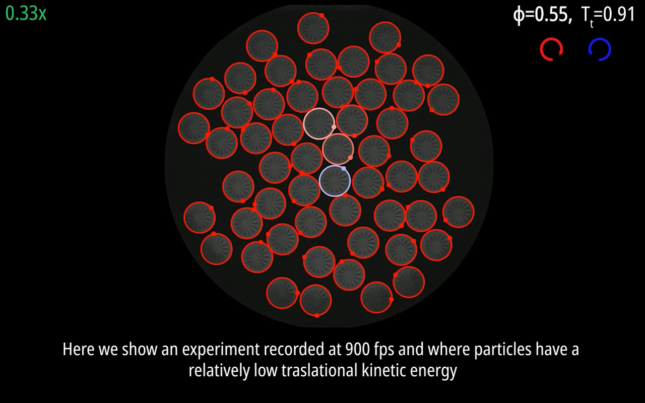
Figure 8: Movie of an experiment (multimedia view) at real-time speed. Each particle is highlighted by a surrounding color circle. Changes in color indicate changes in the spin sign. Blue stands for reverse spin (counter clockwise in this case), whereas red indicates spin in the natural direction imposed by blade tilt (which is the most commmon state at all times, and in this case corresponds to clockwise rotation). Packing fraction $\phi=0.55$ and global mean translational kinetic energy $\overline{T_{t}}=0.91~{}\mathrm{m}\sigma^{2}\mathrm{s}^{-2}$

References

References

- Dombrowski et al. (2004) C. Dombrowski, L. Cisneros, S. Chatkaew, R. E. Goldstein, and J. O. Kessler, “Self-concentration and large-scale coherence in bacterial dynamics,” Physical Review Letters 93, 098103 (2004).
- Marchetti et al. (2013) M. C. Marchetti, J. F. Joanny, S. Ramaswamy, T. B. Liverpool, J. Prost, M. Rao, and R. A. Simha, “Hydrodynamics of soft active matter,” Reviews of Modern Physics 85, 1143–1189 (2013).
- Zhang et al. (2010) H. P. Zhang, A. Be’er, E. L. Florin, and H. L. Swinney, “Collective motion and density fluctuations in bacterial colonies,” Proceedings of the National Academy of Sciences of the United States of America 107, 13626–13630 (2010).
- Petroff, Wu, and Libchaber (2015) A. P. Petroff, X. L. Wu, and A. Libchaber, “Fast-moving bacteria self-organize into active two-dimensional crystals of rotating cells,” Physical Review Letters 114, 158102 (2015).
- Xu et al. (2022) H. Xu, Y. Huang, R. Zhang, and Y. Wu, “Autonomous waves and global motion modes in living active solids,” Nature Physics 19, 46–51 (2022).
- Bowick et al. (2022) M. J. Bowick, N. Fakhri, M. C. Marchetti, and S. Ramaswamy, “Symmetry, thermodynamics, and topology in active matter,” Phys. Rev. X 12, 010501 (2022).
- Nguyen et al. (2014) N. H. Nguyen, D. Klotsa, M. Engel, and S. C. Glotzer, “Emergent collective phenomena in a mixture of hard shapes through active rotation,” Physical Review Letters 112, 075701 (2014), arXiv:1308.2219 .
- Cates and Tailleur (2015) M. E. Cates and J. Tailleur, “Motility-induced phase separation,” Annual Review of Condensed Matter Physics 6, 219–244 (2015), arXiv:1406.3533 .
- Caporusso et al. (2020) C. B. Caporusso, P. Digregorio, D. Levis, L. F. Cugliandolo, and G. Gonnella, “Motility-Induced Microphase and Macrophase Separation in a Two-Dimensional Active Brownian Particle System,” Physical Review Letters 125, 178004 (2020).
- Großmann, Aranson, and Peruani (2020) R. Großmann, I. S. Aranson, and F. Peruani, “A particle-field approach bridges phase separation and collective motion in active matter,” Nature Communications 11, 5365 (2020).
- Liao, Hall, and Klapp (2020) G. J. Liao, C. K. Hall, and S. H. Klapp, “Dynamical self-assembly of dipolar active Brownian particles in two dimensions,” Soft Matter 16, 2208–2223 (2020), arXiv:1907.13430 .
- Gupta et al. (2020) A. Gupta, A. Roy, A. Saha, and S. S. Ray, “Flocking of active particles in a turbulent flow,” Physical Review Fluids 5, 052601(R) (2020).
- Bricard et al. (2015) A. Bricard, J. B. Caussin, D. Das, C. Savoie, V. Chikkadi, K. Shitara, O. Chepizhko, F. Peruani, D. Saintillan, and D. Bartolo, “Emergent vortices in populations of colloidal rollers,” Nature Communications 6, 1–8 (2015).
- Zhang, Sokolov, and Snezhko (2020) B. Zhang, A. Sokolov, and A. Snezhko, “Reconfigurable emergent patterns in active chiral fluids,” Nature Communications 11, 4401 (2020).
- López-Castaño et al. (2022) M. A. López-Castaño, A. Márquez Seco, A. Márquez Seco, A. Rodríguez-Rivas, and F. Vega Reyes, “Chirality transitions in a system of active flat spinners,” Physical Review Research 4, 033230 (2022).
- Mokhtari, Aspelmeier, and Zippelius (2017) Z. Mokhtari, T. Aspelmeier, and A. Zippelius, “Collective rotations of active particles interacting with obstacles,” Europhysics Letters 120, 14001 (2017).
- Farhadi et al. (2018) S. Farhadi, S. Machaca, J. Aird, B. O. Torres Maldonado, S. Davis, P. E. Arratia, and D. J. Durian, “Dynamics and thermodynamics of air-driven active spinners,” Soft Matter 14, 5588–5594 (2018).
- Workamp et al. (2018) M. Workamp, G. Ramirez, K. E. Daniels, and J. A. Dijksman, “Symmetry-reversals in chiral active matter,” Soft Matter 14, 5572–5580 (2018).
- Tsai et al. (2005) J. C. Tsai, F. Ye, J. Rodriguez, J. P. Gollub, and T. C. Lubensky, “A chiral granular gas,” Physical Review Letters 94, 214301 (2005).
- Banerjee et al. (2017) D. Banerjee, A. Souslov, A. G. Abanov, and V. Vitelli, “Odd viscosity in chiral active fluids,” Nature Communications 8, 1573 (2017), arXiv:1702.02393 .
- Hargus, Epstein, and Mandadapu (2021) C. Hargus, J. M. Epstein, and K. K. Mandadapu, “Odd diffusivity of chiral random motion,” Physical Review Letters 127, 178001 (2021).
- Han et al. (2021) M. Han, M. Fruchart, C. Scheibner, S. Vaikuntanathan, J. J. de Pablo, and V. Vitelli, “Fluctuating hydrodynamics of chiral active fluids,” Nature Physics 17, 1260–1269 (2021).
- Avron (1998) J. E. Avron, “Odd viscosity,” J. Stat. Phys. 92, 543 (1998).
- Han et al. (2020) M. Han, M. Fruchart, C. Scheibner, S. Vaikuntanathan, W. Irvine, J. de Pablo, and V. Vitelli, “Statistical mechanics of a chiral active fluid,” (2020), preprint, arXiv:2002.07679 .
- Vega Reyes, López-Castaño, and Rodríguez-Rivas (2022) F. Vega Reyes, M. López-Castaño, and A. Rodríguez-Rivas, “Diffusive regimes in a two-dimensional chiral fluid,” Communications Physics 5, 256 (2022).
- Debets, Löwen, and Janssen (2023) V. E. Debets, H. Löwen, and L. M. Janssen, “Glassy dynamics in chiral fluids,” Physical Review Letters 130, 058201 (2023).
- Ojha et al. (2004) R. P. Ojha, P. A. Lemieux, P. K. Dixon, A. J. Liu, and D. J. Durian, “Statistical mechanics of a gas-fluidized particle,” Nature 427, 521–523 (2004).
- Dyke (1982) M. V. Dyke, An Album of Fluid Motion (Parabolic Press, Stanford, 1982).
- Taneda (1978) S. Taneda, “Visual observations of the flow past a sphere at Reynolds numbers between 10 4 and 10 6,” Journal of Fluid Mechanics 85, 187–192 (1978).
- López-Castaño et al. (2021) M. A. López-Castaño, J. F. González-Saavedra, A. Rodríguez-Rivas, E. Abad, S. B. Yuste, and F. Vega Reyes, “Pseudo-two-dimensional dynamics in a system of macroscopic rolling spheres,” Physical Review E 103, 042903 (2021).
- Kanatani (1979) K.-I. Kanatani, “A micropolar continuum theory for the flow of granular materials,” International Journal of Engineering Science 17, 419–432 (1979).
- Nowak et al. (1998) E. Nowak, J. Knight, E. Ben-Naim, H. Jaeger, and S. Nagel, “Density fluctuations in vibrated granular materials,” Physical Review E 57, 1971–1982 (1998).
- Montanero and Santos (2000) J. M. Montanero and A. Santos, “Computer simulation of uniformly heated granular fluids,” Granular Matter 2, 53–64 (2000), arXiv:0002323 [cond-mat] .
- Allan et al. (2019) D. Allan, C. van der Wel, N. Keim, T. A. Caswell, D. Wieker, R. Verweij, C. Reid, and L. Grueter, “soft-matter/trackpy: Trackpy v0.4.2 (Version v0.4.2),” (2019).
- Bradski (2000) G. Bradski, “The OpenCV Library,” Dr. Dobb’s Journal of Software Tools (2000).
- Crocker and Grier (1996) J. C. Crocker and D. G. Grier, “Methods of Digital Video Microscopy for Colloidal Studies,” Journal of Colloid and Interface Science 179, 298–310 (1996).
- Press et al. (2007) W. H. Press, S. A. Teukolsky, W. T. Vetterling, and B. P. Flannery, Numerical Recipes: The Art of Scientific Computing, 3rd ed. (Cambridge University Press, Cambridge, UK, 2007).
- (38) https://docs.scipy.org/doc/scipy/reference/generated/scipy.signal.correlate.html, SciPy function scipy.signal.correlate.
- Vega Reyes, Santos, and Kremer (2014) F. Vega Reyes, A. Santos, and G. M. Kremer, “Role of roughness on the hydrodynamic homogeneous base state of inelastic spheres,” Physical Review E 89, 020202(R) (2014).
- Goldhirsch I (1993) Z. G. Goldhirsch I, “Clustering instabilities in disspative gases,” Physical Review Letters 70, 1619–1622 (1993).
- Allen and Tildesley (2017) M. P. Allen and D. J. Tildesley, Computer Simulation of Liquids: Second Edition (Oxford University Press, 2017) pp. 58–59.
- Berne (1972) B. J. Berne, “Hydrodynamic theory of the angular velocity autocorrelation function,” The Journal of Chemical Physics 56, 2164–2168 (1972).
- Lowe, Frenkel, and Masters (1995) C. Lowe, D. Frenkel, and A. Masters, “Long-time tails in angular momentum correlations,” The Journal of Chemical Physics 103, 1582 (1995).
- Lokotosh, Malomuzh, and Shakum (2002) T. Lokotosh, N. Malomuzh, and K. Shakum, “Nature of oscillations for the autocorrelation functions for translational and angular velocities of a molecule,” Journal of Molecular Liquids 96–97, 245–263 (2002).
- Kalz et al. (2023) E. Kalz, H. D. Vuijk, J.-U. Sommer, R. Metzler, and A. Sharma, “Oscillatory force autocorrelations in equilibrium odd-diffusive systems,” (2023).
- Welch, Kilmer, and Corwin (2015) K. J. Welch, C. S. G. Kilmer, and E. I. Corwin, “Atomistic study of macroscopic analogs to short-chain molecules,” Physical Review E 91, 022603 (2015).
- de Boeij, Pshenichnikov, and Wiersma (1996) W. P. de Boeij, M. S. Pshenichnikov, and D. A. Wiersma, “System-bath correlation function probed by conventional and time-gated stimulated photon echo,” The Journal of Physical Chemistry 100 (1996).
- Labous, Rosato, and Dave (1997) L. Labous, A. D. Rosato, and R. N. Dave, “Measurements of collisional properties of spheres using high-speed video analysis,” Physical Review E - Statistical Physics, Plasmas, Fluids, and Related Interdisciplinary Topics 56, 5717–5725 (1997).
- Jiang et al. (2020) Z. Jiang, J. Du, C. Rieck, A. Bück, and E. Tsotsas, “PTV experiments and DEM simulations of the coefficient of restitution for irregular particles impacting on horizontal substrates,” Powder Technology 360, 352–365 (2020).
- Tierno and Snezhko (2021) P. Tierno and A. Snezhko, “Transport and assembly of magnetic surface rotors,” ChemNanoMat 7, 881 (2021).
- Lee and Hsu (1996) H.-Y. Lee and I.-S. Hsu, “Particle Spinning Motion during Saltating Process,” Journal of Hydraulic Engineering 122, 587–590 (1996).
- Lu et al. (2021) C. Lu, R. Zhu, F. Yu, X. Jiang, Z. Liu, L. Dong, Q. Hua, and Z. Ou, “Gear rotational speed sensor based on FeCoSiB/Pb(Zr,Ti)O3 magnetoelectric composite,” Measurement: Journal of the International Measurement Confederation 168, 108409 (2021).
- Scholz et al. (2018) C. Scholz, S. Jahanshahi, A. Ldov, and H. Löwen, “Inertial delay of self-propelled particles,” Nature Communications 9, 5156 (2018), arXiv:1807.04357 .
- Grasselli, Bossis, and Morini (2015) Y. Grasselli, G. Bossis, and R. Morini, “Translational and rotational temperatures of a 2D vibrated granular gas in microgravity,” European Physical Journal E 38, 8 (2015).
- Barros, Hiltbrand, and Longmire (2018) D. Barros, B. Hiltbrand, and E. K. Longmire, “Measurement of the translation and rotation of a sphere in fluid flow,” Experiments in Fluids 59, 104 (2018).
- Zimmermann et al. (2011) R. Zimmermann, Y. Gasteuil, M. Bourgoin, R. Volk, A. Pumir, and J. F. Pinton, “Tracking the dynamics of translation and absolute orientation of a sphere in a turbulent flow,” Review of Scientific Instruments 82, 033906 (2011).
- Hagemeier, Bück, and Tsotsas (2015) T. Hagemeier, A. Bück, and E. Tsotsas, “Estimation of particle rotation in fluidized beds by means of PTV,” Procedia Engineering 102, 841–849 (2015).
- Tsai (1987) R. Y. Tsai, “A Versatile Camera Calibration Technique for High-Accuracy 3D Machine Vision Metrology Using Off-the-Shelf TV Cameras and Lenses,” IEEE Journal on Robotics and Automation 3, 323–344 (1987).
- Adrian (1991) R. J. Adrian, “Particle-Imaging Techniques for Experimental Fluid Mechanics,” Annual Review of Fluid Mechanics 23, 261–304 (1991).
- Helminiak et al. (2018) N. S. Helminiak, D. S. Helminiak, V. Cariapa, and J. P. Borg, “Resolving the angular velocity of two-dimensional particle interactions induced within a rotary tumbler,” Journal of Visualization 21, 779–793 (2018).
- Papoulis (1978) A. Papoulis, The Fourier Integral and Its Applications (Mcraw-Hill, New York, 1978).
- Van der Walt and Aivazis (2011) S. Van der Walt and M. Aivazis, “The NumPy Array: A Structure for Efficient Numerical Computation, Computing in Science & Engineering,” Computing in Science and Engineering 13, 22–30 (2011).
- Vega Reyes, López-Castaño, and Márquez Seco (2021) F. Vega Reyes, M. A. López-Castaño, and A. Márquez Seco, “Angular tracking source code,” https://github.com/fvegar/blades/ (2021).
- Savin and Doyle (2005) T. Savin and P. S. Doyle, “Static and dynamic errors in particle tracking microrheology,” Biophysical Journal 88, 623–638 (2005).
- Feng, Goree, and Liu (2011) Y. Feng, J. Goree, and B. Liu, “Errors in particle tracking velocimetry with high-speed cameras,” Review of Scientific Instruments 82, 053707 (2011), arXiv:1104.3540 .
- Sciacchitano (2019) A. Sciacchitano, “Uncertainty quantification in particle image velocimetry,” Measurement Science and Technology 30, 092001 (2019).