Two-Loop Hexa-Box Integrals for Non-Planar Five-Point One-Mass Processes

Abstract

We present the calculation of the three distinct non-planar hexa-box topologies for five-point one-mass processes. These three topologies are required to obtain the two-loop virtual QCD corrections for two-jet-associated W, Z or Higgs-boson production. Each topology is solved by obtaining a pure basis of master integrals and efficiently constructing the associated differential equation with numerical sampling and unitarity-cut techniques. We present compact expressions for the alphabet of these non-planar integrals, and discuss some properties of their symbol. Notably, we observe that the extended Steinmann relations are in general not satisfied. Finally, we solve the differential equations in terms of generalized power series and provide high-precision values in different regions of phase space which can be used as boundary conditions for subsequent evaluations.

1 Introduction

The evaluation of Feynman integrals is a central problem one needs to address when computing loop corrections in any perturbative quantum field theory (QFT). Modern approaches to the calculation of loop corrections to various quantities in QFT proceed by decomposing them into a sum of products of algebraic coefficients and master integrals. The algebraic coefficients depend on the loop order, the quantity being computed and the QFT under consideration. The master integrals, on the other hand, only depend on the underlying kinematics and loop order. The evaluation of master integrals is thus an interesting problem on its own.

Despite receiving a lot of attention in recent years, the calculation of Feynman integrals still poses a major challenge in obtaining two-loop corrections for processes of great physical interest. At the multi-leg and multi-loop frontier, the complete set of master integrals required for the scattering of five massless particles has been computed Gehrmann:2015bfy ; Papadopoulos:2015jft ; Abreu:2018aqd ; Chicherin:2018old ; Chicherin:2020oor , which has led to a large number of new analytic two-loop amplitudes in both supersymmetric theories and in QCD Abreu:2018aqd ; Chicherin:2018yne ; Abreu:2019rpt ; Chicherin:2019xeg ; Badger:2018enw ; Abreu:2018zmy ; Abreu:2019odu ; Abreu:2021oya ; Badger:2019djh ; Chawdhry:2019bji ; Abreu:2020cwb ; Chawdhry:2020for ; Agarwal:2021grm ; Chawdhry:2021mkw ; Badger:2021imn .

More recently, all planar master integrals relevant for the scattering of a massive particle and four-massless ones were computed Abreu:2020jxa ; Canko:2020ylt . These results have already allowed the calculation of the two-loop QCD corrections to the $u\bar{d}\to W^{+}b\bar{b}$ process Badger:2021nhg at leading color, as well as the calculation of new two-loop form factors in planar $\mathcal{N}=4$ SYM Guo:2021bym . However, for other important physical processes at hadron colliders, such as the production of a Z or Higgs boson in association with two jets, as well as sub-leading color effects in the production of a W boson in association with two jets, the planar integrals considered in refs. Abreu:2020jxa ; Canko:2020ylt are not sufficient. To extend the results of ref. Abreu:2020jxa beyond the planar limit there are five new topologies of master integrals that must be computed. These can be grouped into two sets: there are three distinct hexa-box topologies, and two distinct double-pentagon topologies. While one of the hexa-box topologies has been considered previously Papadopoulos:2019iam , in this paper we compute for the first time the full set of hexa-box topologies.

Our calculation of the hexa-box master integrals follows the approach used in ref. Abreu:2020jxa , which gives us detailed insight into the analytic structure of the master integrals but also allows one to numerically evaluate the master integrals at any phase-space point. We start by constructing differential equations for the master integrals Kotikov:1990kg ; Kotikov:1991pm ; Bern:1993kr ; Remiddi:1997ny ; Gehrmann:1999as , choosing a basis of ‘pure’ master integrals ArkaniHamed:2010gh so that the differential equations take a particularly simple ‘canonical’ form Henn:2013pwa , which only involves $\mathrm{d}\log$ forms. In practice, we construct the basis with a heuristic approach that is validated by constructing the differential equation and observing the canonical form. Contrary to the massless five-point case Chicherin:2017dob , we find that the collection of $\mathrm{d}\log$ forms which appear in the differential equations is not given by the permutation closure of those arising in the planar topologies Abreu:2020jxa . Indeed, we find a new class of square root, not associated to a momentum-space gram determinant. In order to determine the remaining $\mathrm{d}\log$ forms, we use the approach of ref. Abreu:2020jxa and consider much simpler differential equations where the propagators are put on shell. To obtain the analytic form of the differential equation we use the numerical sampling method of ref. Abreu:2018rcw , which trivializes the integral reduction of the differential equations and can be implemented over finite fields vonManteuffel:2014ixa ; Peraro:2016wsq .

Once the canonical differential equation is known, it is trivial to determine the so-called ‘symbol’ Goncharov:2010jf ; Duhr:2011zq ; Duhr:2012fh of the master integrals, which gives valuable insight into the analytic structure of the master integrals in a compact format. In a nutshell, these integrals evaluate to multi-valued functions with complicated branch-cut structures, and the symbol encodes the information about the position of all logarithmic singularities. The symbol is built out of ‘letters’, which are algebraic functions of the kinematic variables that vanish at the logarithmic singularities of the integrals. The symbol contains non-trivial information about the analytic properties of the master integrals and scattering amplitudes. For instance, the analytic form of the letters can be used to greatly simplify the calculation of loop amplitudes Abreu:2018zmy ; Abreu:2019odu . The symbols also encode the discontinuities of Feynman integrals, which are constrained by physical considerations. As expected, we observe that the symbols of the hexa-box integrals satisfy the Steinmann relations Steinmann ; Steinmann2 ; Cahill:1973qp ; Caron-Huot:2016owq ; Dixon:2016nkn . However, interestingly, we find that the ‘extended Steinmann relations’ Caron-Huot:2018dsv are in general not satisfied.

The differential equation can also be used to numerically evaluate the master integrals. One approach would be to analytically solve the differential equation in terms of multiple polylogarithms (MPLs). However, given the high number of variables and the weight of the MPLs, for the hexa-box integrals we consider this would lead to lengthy expressions which are specific to a given phase-space region and highly non-trivial to analytically continue. Instead, we numerically solve the differential equations using generalized power series Francesco:2019yqt ; Hidding:2020ytt , a method which was already shown to be suitable for the planar two-loop five-point one-mass integrals Abreu:2020jxa . Compared to Monte-Carlo based approaches Smirnov:2015mct ; Borowka:2017idc ; Capatti:2019ypt ; Capatti:2019edf ; Runkel:2019yrs , the numerical solution of the differential equation in terms of generalized power series allows to obtain high-precision results (see also the approaches of refs. Mandal:2018cdj ; Liu:2021wks ), which, for instance, means that we can evaluate the integrals in singular regions of phase space to arbitrary precision. To obtain numerical values for the hexa-box integrals, we determine a set of initial conditions by requiring that the integrals are free of spurious branch cuts in their Euclidean region. These initial conditions correspond to the value of the integrals at a Euclidean phase-space point, and they were obtained to more than 100 digits with an in-house code. We then use the code of ref. Hidding:2020ytt to obtain high-precision numerical values in different regions of phase space, which can themselves be used as initial conditions for subsequent evaluations.

To facilitate the use of our results, we include a set of ancillary files which contain all our analytic and numerical results. For each of the three hexa-box topologies, we include a file with the definition of the pure basis, anc/*/*_pure_basis.m, and a file with a graphical representation of the master integrals anc/*/*_graphs.m. The differential equations can be assembled from the list of matrices in anc/*/*_connection.m and the alphabet in anc/alphabet.m. We also include the file anc/usageExample.m which illustrates the use of the ancillary files, and allows to compute the symbols of all master integrals to the desired weight.

The paper is structured as follows. In section 2 we describe the kinematics relevant for the master integrals we will be computing and introduce quantities such as Gram determinants that will be important for the construction of the differential equations. In section 3 we define the hexa-box topologies. Next, in section 4 we discuss the canonical differential equations and present the pure bases for each topology. In section 5 we discuss the symbol alphabet, the analytic form of the differential equations and some properties of the symbols of the hexa-box integrals. Finally, in section 6 we discuss the numerical solution of the differential equations, before we present our conclusions in section 7.

2 Scattering Kinematics and Notation

We consider the scattering of five particles, four of which are massless. We denote their momenta by $p_{i},$ $i=1,\ldots,5$, which satisfy the momentum conservation $\sum_{i=1}^{5}p_{i}=0$ and, without loss of generality, we take $p_{1}^{2}\neq 0$, and $p_{i}^{2}=0$ for $i=2,\ldots,5$. The Mandelstam variables $s_{ij}=(p_{i}+p_{j})^{2}$ for arbitrary $i$ and $j$ can all be written as linear combinations of the six variables

$$\vec{s}=\{p_{1}^{2}{}\,,s_{12}\,,s_{23}\,,s_{34}\,,s_{45}\,,s_{15}\}\,.$$ (1)

These six variables are however not sufficient to specify a point in the five-particle phase space. Indeed, this space is separated into two halves which are mapped onto each other by a space-time parity transformation. The parity label of each point can be captured by the parity-odd contraction with the Levi-Civita tensor

$${\rm tr}_{5}{}=4i\varepsilon_{\alpha\beta\gamma\delta}\,p_{1}^{\alpha}p_{2}^{\beta}p_{3}^{\gamma}p_{4}^{\delta}\,.$$ (2)

A ubiquitous set of quantities that appears when describing the kinematics of a scattering process are the Gram determinants one can form with (subsets of) the momenta $p_{i}$. They are given by the determinants of the Gram matrix $G(q_{1},\ldots,q_{n})$, which we define as

$$G(q_{1},\ldots,q_{n})=2\,V^{T}(q_{1},\ldots,q_{n})\,g\,V(q_{1},\ldots,q_{n})=2\,\{q_{i}\cdot q_{j}\}_{i,j\in\{1,\ldots,n\}}\,,$$ (3)

where $V(q_{1},\ldots,q_{n})$ is a $4\times n$ matrix whose columns are the vectors $q_{i}$. For concreteness, in this paper we use the metric $g=\mathrm{diag}(+,-,-,-)$, which we extend with further minus signs when working with $D$-dimensional momenta. It is clear from eq. 3 that the Gram determinants are just polynomials in the Mandelstam variables. We will be particularly interested in the three-point Gram determinant

$$\begin{split}\Delta_{3}=&\,-\det G(p_{1},p_{2}+p_{3})\\ =&\,s_{23}^{2}+s_{45}^{2}+p_{1}^{4}-2s_{23}s_{45}-2p_{1}^{2}{}s_{23}-2p_{1}^{2}{}s_{45}\\ =&\,\lambda(p_{1}^{2}{},s_{23},s_{45})\,,\end{split}$$ (4)

where $\lambda(a,b,c)=a^{2}+b^{2}+c^{2}-2ab-2ac-2bc$ is the Källén function, and in the five-point Gram determinant

$$\begin{split}\Delta_{5}=&\,\det G(p_{1},p_{2},p_{3},p_{4})\\ =&\,(s_{12}s_{15}-s_{12}s_{23}-p_{1}^{2}{}s_{34}-s_{15}s_{45}+s_{34}s_{45}+s_{23}s_{34})^{2}\\ &\,-4s_{23}s_{34}s_{45}(p_{1}^{2}{}-s_{12}-s_{15}+s_{34})\,.\end{split}$$ (5)

The five-point Gram determinant $\Delta_{5}$ is closely related to the ${\rm tr}_{5}{}$ defined in eq. 2, as we have that

$$\Delta_{5}={\rm tr}_{5}^{2}\,.$$ (6)

It is then very tempting to identify ${\rm tr}_{5}{}$ with $\sqrt{\Delta_{5}}$, but one must take care with this identification. While ${\rm tr}_{5}{}$ is a square root of $\Delta_{5}$, the branch choice (correspondingly the sign) is fixed by the underlying set of momenta defining the phase-space point. In contrast, the branch choice/sign of $\sqrt{\Delta_{5}}$ can conveniently be fixed by the standard prescription of the square-root map. With this convention $\sqrt{\Delta_{5}}$ depends only on the $s_{ij}$ themselves and not on ${\rm tr}_{5}{}$. Consequently, ${\rm tr}_{5}{}$ is odd under parity transformations while $\sqrt{\Delta_{5}}$ is invariant, and to relate ${\rm tr}_{5}{}$ to $\sqrt{\Delta_{5}}$ we must encode the different choices of branch of the square root. To avoid these complications, and because it is sufficient for the purpose of this paper, we will avoid referring to ${\rm tr}_{5}{}$ and instead use $\Delta_{5}$ and $\sqrt{\Delta_{5}}$.

Another quantity that will appear throughout this paper and which is closely related to $\Delta_{5}$ is

$$\begin{split}\Sigma_{5}=&\,(s_{12}s_{15}-s_{12}s_{23}-s_{15}s_{45}+s_{34}s_{45}+s_{23}s_{34})^{2}-4s_{23}s_{34}s_{45}(s_{34}-s_{12}-s_{15})\,.\end{split}$$ (7)

In particular we note that in the limit where $p_{1}^{2}\to 0$ the two quantities coincide, that is

$$\Sigma_{5}=\Delta_{5}\qquad\text{for}\qquad p_{1}^{2}=0\,,$$

as is manifest from eqs. 5 and 7. We will see below how this polynomial appears in the construction of the pure basis.

Given a phase-space point $P=\{p_{1},p_{2},p_{3},p_{4},p_{5}\}$, it is natural to consider the points obtained by permuting the massless legs. More formally, let us consider the different points $\sigma(P)=\{p_{1},p_{\sigma(2)},p_{\sigma(3)},p_{\sigma(4)},p_{\sigma(5)}\}$ where $\sigma\in S_{4}$ corresponds to a permutation of $\{2,3,4,5\}$. The action of $\sigma$ on the $s_{ij}$ is trivially defined as $\sigma(s_{ij})=(p_{\sigma(i)}+p_{\sigma(j)})^{2}$. While $\Delta_{5}$ is invariant under these permutations, $\Delta_{3}$ is not. We find that there are three independent permutations of $\Delta_{3}$, namely

$$\Delta_{3}^{(1)}=\lambda(p_{1}^{2}{},s_{23},s_{45})\,,\qquad\Delta_{3}^{(2)}=\lambda(p_{1}^{2}{},s_{24},s_{35})\qquad\text{and}\qquad\Delta_{3}^{(3)}=\lambda(p_{1}^{2}{},s_{25},s_{34})\,.$$ (8)

The polynomial $\Sigma_{5}$ defined in eq. 7 is also not invariant under a general $\sigma\in S_{4}$, and we find that it appears in six different permutations, which we denote by $\Sigma_{5}^{(k)}$, for $k=1,\ldots,6$, with $\Sigma_{5}^{(1)}=\Sigma_{5}$.

3 Hexa-box Topologies

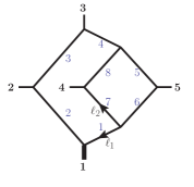
(a) $I_{\rm hb}^{[\textrm{mzz}]}[\vec{\nu}]$

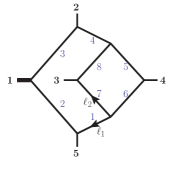
(b) $I_{\rm hb}^{[\textrm{zmz}]}[\vec{\nu}]$

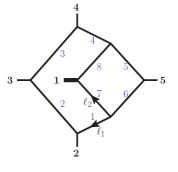
(c) $I_{\rm hb}^{[\textrm{zzz}]}[\vec{\nu}]$

Figure 1: Two-loop five-point one-mass non-planar hexa-box topologies. The thick external line with label 1 denotes the massive external leg.

There are three non-planar hexa-box topologies with a single massive external leg that are not related by a relabelling of the external momenta. These three topologies are depicted in fig. 1. We denote them by $I_{\rm hb}^{[f]}$, with $f\in\{\textrm{mzz},\textrm{zmz},\textrm{zzz}\}$ distinguishing the mass assignment for the three external legs of the hexagon sub-loop: they can all have zero mass (zzz), the middle leg can be massive (zmz), or the first leg can be massive (mzz). Each topology defines a linear space $Y^{[f]}$ of integrals corresponding to linear combinations of integrals of the form

$$I_{\rm hb}^{[f]}[\vec{\nu}]=\int\frac{{\rm d}^{D}\ell_{1}}{i\pi^{D/2}}\frac{{\rm d}^{D}\ell_{2}}{i\pi^{D/2}}\frac{\rho_{9,f}^{-\nu_{9}}\,\,\rho_{10,f}^{-\nu_{10}}\,\,\rho_{11,f}^{-\nu_{11}}}{\rho_{1,f}^{\nu_{1}}\,\,\rho_{2,f}^{\nu_{2}}\,\,\rho_{3,f}^{\nu_{3}}\,\,\rho_{4,f}^{\nu_{4}}\,\,\rho_{5,f}^{\nu_{5}}\,\,\rho_{6,f}^{\nu_{6}}\,\,\rho_{7,f}^{\nu_{7}}\,\,\rho_{8,f}^{\nu_{8}}}\,,$$ (9)

where we set $D=4-2\epsilon$. Each element in this spanning set is distinguished by a set of integer values $\vec{\nu}$, with the restriction that $\nu_{9},\nu_{10},\nu_{11}\leq 0$. Concretely, the propagator variables ($\rho_{i,f},\,i=1,\ldots,8$) and the irreducible scalar products ($\rho_{i,f},\,i=9,\dots,11$) are defined for each topology as

$$\begin{split}\vec{\rho}_{\textrm{mzz}}=&\left\{\ell_{1}^{2},(\ell_{1}+p_{1})^{2},(\ell_{1}+p_{1}+p_{2})^{2},(\ell_{1}+p_{1}+p_{2}+p_{3})^{2},(\ell_{1}+\ell_{2}-p_{5})^{2},(\ell_{1}+\ell_{2})^{2},\right.\\ &\quad\left.\ell_{2}^{2},(\ell_{2}+p_{4})^{2},(\ell_{2}+p_{1})^{2},(\ell_{1}+p_{4})^{2},(\ell_{2}+p_{1}+p_{2})^{2}\right\},\\[5.69054pt] \vec{\rho}_{\textrm{zmz}}=&\left\{\ell_{1}^{2},(\ell_{1}+p_{5})^{2},(\ell_{1}+p_{5}+p_{1})^{2},(\ell_{1}+p_{5}+p_{1}+p_{2})^{2},(\ell_{1}+\ell_{2}-p_{4})^{2},(\ell_{1}+\ell_{2})^{2},\right.\\ &\quad\left.\ell_{2}^{2},(\ell_{2}+p_{3})^{2},(\ell_{2}+p_{5})^{2},(\ell_{1}+p_{3})^{2},(\ell_{2}+p_{5}+p_{1})^{2}\right\},\\[5.69054pt] \vec{\rho}_{\textrm{zzz}}=&\left\{\ell_{1}^{2},(\ell_{1}+p_{2})^{2},(\ell_{1}+p_{2}+p_{3})^{2},(\ell_{1}+p_{2}+p_{3}+p_{4})^{2},(\ell_{1}+\ell_{2}-p_{5})^{2},(\ell_{1}+\ell_{2})^{2},\right.\\ &\quad\left.\ell_{2}^{2},(\ell_{2}+p_{1})^{2},(\ell_{2}+p_{2})^{2},(\ell_{1}+p_{1})^{2},(\ell_{2}+p_{2}+p_{3})^{2}\right\}.\end{split}$$ (10)

In fig. 1, where we assume that all external momenta are incoming, we include the index associated with each propagator and the routing of the loop momenta $\ell_{1}$ and $\ell_{2}$.

The integrals specified in eq. 9 define a space of integrals $Y^{[f]}$ associated with each topology. In this paper we compute a basis of these spaces, i.e., a set of master integrals associated with each topology. The projection of any element of this space onto the basis of master integrals can be algorithmically constructed with integration-by-parts (IBP) identities Chetyrkin:1981qh ; Tkachov:1981wb ; Laporta:2001dd . The dimensions of the bases are

$$\begin{split}&\text{dim}(Y^{[\textrm{mzz}]})=86,\ \ \ \ \text{dim}(Y^{[\textrm{zmz}]})=86,\ \ \ \ \text{dim}(Y^{[\textrm{zzz}]})=135.\end{split}$$ (11)

While it is trivial to find some basis for each of these spaces, one of the main results of this paper will be the construction of pure bases, which have particularly nice properties. This will be discussed in detail in the next section.

Figure 2: Propagator structures of two-loop five-point non-planar master integrals in the hexa-box topologies.

Even though the dimensions given in eq. (LABEL:eq:masterCount) are rather large, there is a substantial overlap between these different spaces, as the same master integrals can appear in different topologies. Furthermore, some of the master integrals have been computed previously: the planar five-point integrals were given in ref. Abreu:2020jxa , and the integrals associated with Feynman diagrams with four external legs in refs. Henn:2014lfa ; Caola:2014lpa ; Gehrmann:2015ora . The master integrals that appear for the first time in the three non-planar hexa-box topologies are depicted in fig. 2. Finally, we note that a full set of master integrals for topology $I^{[\textrm{mzz}]}_{\rm hb}[\vec{\nu}]$ has already been computed in ref. Papadopoulos:2019iam .

4 Canonical Differential Equation and Pure Basis

4.1 Canonical Differential Equation

A particularly powerful method to evaluate Feynman integrals with many scales is by solving the differential equations they satisfy Kotikov:1990kg ; Kotikov:1991pm ; Bern:1993kr ; Remiddi:1997ny ; Gehrmann:1999as ; Henn:2013pwa . Let ${\bf I}$ be a vector containing the set of master integrals associated with a given topology (such as the mzz, zmz or zzz hexa-boxes). We consider the master integrals as functions of the Mandelstam variables $\vec{s}$, and treat the dimensional regulator $\epsilon=(4-D)/2$ as a parameter. The vector ${\bf I}$ satisfies the differential equation

$${\rm d}{\bf I}=\,\overline{\bf M}\,{\bf I}\,,$$ (12)

where the connection $\overline{\bf M}$ is a matrix of differential forms which depends rationally on the dimensional regulator $\epsilon$. The form of the differential equation (12) follows from the fact that differential operators generate linear combinations of elements in the space $Y^{[f]}$ associated with each topology, which can then be mapped back into the basis ${\bf I}$. For complicated enough integrals, this procedure can be a bottleneck in determining the differential equations.

The construction of the differential equation can be simplified in two ways. First, it is clear that the form of the connection $\overline{\bf M}$ depends on the basis ${\bf I}$, and $\overline{\bf M}$ will be particularly simple if a basis of so-called ‘pure’ functions is chosen Henn:2013pwa . For such a basis, the connection can be written as

$$\overline{\bf M}=\epsilon\,{\bf M}\,,\qquad{\bf M}=\sum_{\alpha}\,M_{\alpha}\,{\rm d}\log{(W_{\alpha})}\,,$$ (13)

where the elements of the matrices $M_{\alpha}$ are rational numbers and the $W_{\alpha}$ are algebraic functions of the Mandelstam variables $\vec{s}$, known as the ‘letters’ of the ‘(symbol) alphabet’ $\mathcal{A}$ associated with the topology under consideration. If the connection $\overline{\bf M}$ takes the form given in eq. 13, the differential equation is said to be in canonical form.

The second simplification is in the way the connection ${\bf M}$ is determined once a pure basis has been found Abreu:2018rcw ; Abreu:2018aqd ; Abreu:2020jxa . Instead of performing fully analytic IBP reductions for the whole system, we determine the new letters from much simpler ‘cut’ differential equations, where all integrals that do not contain the set of cut propagators are set to zero. Once all the letters $W_{\alpha}$ have been determined, the matrices $M_{\alpha}$ are computed from fully numerical IBP reductions.

In the remainder of this section, we will discuss the construction of the pure bases of master integrals for the non-planar five-point one-mass integrals of fig. 2. The determination of the associated connections ${\bf M}$ will be left to the next section. In both cases we will find it useful to consider a ‘random-direction differential equation’ Abreu:2020jxa , which allows us to replace the connection ${\bf M}$ by an algebraic function of the kinematics and dimensional regulator. More explicitly, we choose an arbitrary direction $\vec{c}$ in the six-dimensional space of the Mandelstam variables and compute

$$\vec{c}\cdot\nabla_{\vec{s}}\,{\bf I}=C(\epsilon,\vec{s}\,){\bf I}\,,$$ (14)

where $\nabla_{\vec{s}}=\{\frac{\partial}{\partial p_{1}^{2}},\frac{\partial}{\partial s_{12}},…\}$ is the gradient operator with respect to the Mandelstam variables in eq. 1. For a pure basis, i.e., in the case of a canonical differential equation, $C(\epsilon,\vec{s}\,)$ is given by

$$C(\epsilon,\vec{s}\,)=\epsilon\,\sum_{\alpha}M_{\alpha}\,\vec{c}\cdot\nabla_{\vec{s}}\,\log(W_{\alpha})\,,$$ (15)

and, assuming the vector $\vec{c}$ is generic, it captures the dependence of ${\bf M}$ on the $M_{\alpha}$ and $W_{\alpha}$. In practice, we find the matrix $C(\epsilon,\vec{s}\,)$ particularly useful as it can be evaluated on numerical kinematic configurations, by performing numerical IBP reductions of the left-hand side of eq. 14.

4.2 Pure Basis

The construction of a pure basis for multi-scale Feynman integrals remains challenging, despite much recent progress Lee:2014ioa ; Prausa:2017ltv ; Gituliar:2017vzm ; Meyer:2017joq ; Abreu:2018rcw ; Wasser:2018qvj ; Abreu:2018aqd ; Chicherin:2018old ; Dlapa:2020cwj ; Henn:2020lye ; Abreu:2020jxa . Moreover, starting from five external legs, four-dimensional analyzes are often not sufficient, see e.g. refs. Abreu:2018aqd ; Chicherin:2018old . In this section we discuss how a basis of pure master integrals for all the integrals in fig. 2 was constructed. As we explain below, this process requires the calculation of numerical IBP reductions. These were obtained with two publicly available codes, Kira 1.2 Maierhoefer:2017hyi and FIRE6 Smirnov:2019qkx .

Throughout this section, we will often use the functions $\mu_{ij}$ when constructing pure integrals. These correspond to contractions of the components of the loop momenta beyond four dimensions, which we denote $\ell^{(D-4)}_{i}$. Explicitly,

$$\mu_{ij}=\ell^{(D-4)}_{i}\cdot\ell^{(D-4)}_{j}\,.$$ (16)

These functions can also be written as polynomials in the $\rho_{i,f}$ and the Mandelstam variables $\vec{s}$, see eqs. 1 and 10. The latter representation is more convenient if one wants to rewrite integrals defined with the help of these functions as members of the vector spaces $Y^{[f]}$. For convenience and to remove any ambiguity related to conventions, we provide a routine to compute the functions $\mu_{11}$, $\mu_{22}$ and $\mu_{12}$ in the ancillary file anc/determinants.m .

The integrals listed in fig. 2 can be grouped into two classes: the cases for which the number of master integrals is the same as in the massless limit $p_{1}^{2}\rightarrow 0$, and the cases with an increased number of master integrals. For instance, for the three independent hexa-box topologies on the top row of fig. 2 we find that the number of master integrals is the same. In such cases, the trivial generalization of the pure basis from the massless case Abreu:2018rcw to the massive case gives a complete set of pure master integrals. Despite not being the main difficulty in constructing a complete basis of master integrals, we note that the pure bases we present here for these integrals (which we list below) are particularly compact.

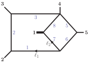
Figure 3: Penta-box with 6 master integrals.

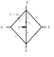
Figure 4: Double-box with 4 master integrals.

The cases for which the master-integral count changes are more challenging to handle. These cases are the penta-box diagram depicted in fig. 3 and the double-box integral shown in fig. 4. In order to determine a basis of pure integrals (beyond those corresponding to generalizations of the massless case) we use a similar approach in both cases. We start by constructing educated guesses for pure master integrals by studying their leading singularities Cachazo:2008vp , the goal being to check if they can be written as $d{\rm log}$ forms with unit leading singularity (see e.g. Henn:2014qga ). In complicated cases, this analysis can be done under the condition that all of the inverse propagators are set to zero (i.e., on their ‘maximal cut’). Working on the maximal cut has another benefit: the differential equations on the maximal cut are much simpler, as all integrals that do not involve all the cut propagators are set to zero. We thus verify if, under these cut conditions, we obtain a canonical differential equation of the form of eq. 13 or eq. 15. This can be done fully numerically, by setting the Mandelstam variables and the dimensional regulator to generic numerical values. In fact, to be more precise, at this stage we simply check that the $\epsilon$ dependence factorizes in the matrix $C(\epsilon,\vec{s}\,)$ of eq. 15, and we cannot yet guarantee that it only involves $d{\rm log}$ forms and matrices of rational numbers. Nevertheless, for now we assume that $\epsilon$ factorization implies purity of the basis we are constructing (in the next section we discuss how this assumption is verified). Once we have built enough pure master integrals on the maximal cut, we start releasing cut conditions and check, numerically, if the $\epsilon$ dependence still factorizes in the differential equation. If it is not the case, we correct the candidate pure integral with terms proportional to the propagator which is no longer set to zero.

Either by generalizing the pure integrals from $p_{1}^{2}=0$ to $p_{1}^{2}\neq 0$ or by following the steps above, we constructed bases of master integrals for all the diagrams depicted in fig. 2. Before listing the integrands corresponding to the pure bases, let us discuss a particular example in more detail, as it will illuminate the appearance of the (square-root of the) polynomial in eq. 7. We consider the double-box integral of fig. 4,

$$I_{\rm db}=\int\frac{{\rm d}^{D}\ell_{1}}{i\pi^{D/2}}\frac{{\rm d}^{D}\ell_{2}}{i\pi^{D/2}}\frac{\mathcal{N}^{(1)}}{(\ell_{1}+p_{2})^{2}(\ell_{1}+p_{2}+p_{3})^{2}(\ell_{1}+\ell_{2}-p_{5})^{2}(\ell_{1}+\ell_{2})^{2}\ell_{2}^{2}(\ell_{2}+p_{1})^{2}}\,.$$ (17)

By analogy with the planar case Henn:2013pwa ; Henn:2014qga , given that it is a double-box integral we expect that the integral should be pure for some function $\mathcal{N}^{(1)}$ that depends only on the external kinematics and, furthermore, that it should be possible to compute this function by studying the leading singularity of the scalar integral in exactly four dimensions. In order to do this, we consider a loop-by-loop approach and write

$$I_{\rm db}\sim\mathcal{N}^{(1)}\int\frac{{\rm d}^{4}\ell_{2}}{\ell_{2}^{2}(\ell_{2}+p_{1})^{2}}\left(\int\frac{{\rm d}^{4}\ell_{1}}{(\ell_{1}+p_{2})^{2}(\ell_{1}+p_{2}+p_{3})^{2}(\ell_{1}+\ell_{2}-p_{5})^{2}(\ell_{1}+\ell_{2})^{2}}\right)\,,$$ (18)

where we did not keep track of conventional numerical normalization factors. The innermost integral over the loop momentum $\ell_{1}$ corresponds to a so-called ‘two-mass easy’ box in four dimensions. It is well know that such an integral has a $d{\rm log}$ representation Arkani-Hamed:2016byb , and that its leading singularity is (see e.g. Abreu:2017ptx )

$${\cal R}_{\rm box} =\frac{1}{(\ell_{2}-p_{2}-p_{3})^{2}(\ell_{2}+p_{1}+p_{3}+p_{4})^{2}-(\ell_{2}-p_{2})^{2}(\ell_{2}+p_{1}+p_{4})^{2}}.$$ (19)

To proceed, we use the factorization properties of this leading singularity Bern:2014kca , i.e. we define momenta $q$ and $\bar{q}$ such that

$$q\cdot(\ell_{2}-p_{2})=\langle p_{3}|(/{\ell}_{2}-/{p}_{2})|p_{5}]\quad\textrm{and}\quad\bar{q}\cdot(\ell_{2}-p_{2})=[p_{3}|(/{\ell}_{2}-/{p}_{2})|p_{5}\rangle,$$ (20)

which allow us to factorize the denominator of ${\cal R}_{\rm box}$,

$${\cal R}_{\rm box} =\frac{1}{(q\cdot[\ell_{2}-p_{2}])\,(\bar{q}\cdot[\ell_{2}-p_{2}])}.$$ (21)

We are now left with the task of determining $\mathcal{N}^{(1)}$ such that the differential form

$$\omega=\frac{\mathcal{N}^{(1)}\,{\rm d}^{4}\ell_{2}}{(\ell_{2})^{2}(\ell_{2}+p_{1})^{2}(q\cdot[\ell_{2}-p_{2}])\,(\bar{q}\cdot[\ell_{2}-p_{2}])}$$ (22)

has unit leading singularity. This can be achieved in a simple and enlightening manner by using the embedding-space formalism of ref. SimmonsDuffin:2012uy , see also refs. Caron-Huot:2014lda ; Abreu:2017ptx for applications to Feynman integrals.

This formalism upgrades the 4-dimensional form to a form in a 6-dimensional projective space which is integrated over the light cone. We label points in the 6-dimensional embedding space with capital letters. A vector $V$ in embedding space is written in terms of a four-dimensional vector $v$ and two light-cone components, i.e.,

$$V=(v,V^{+},V^{-})\,.$$ (23)

The scalar product between two embedding-space vectors $V$ and $W$ is defined as

$$(VW)=-2(v\cdot w)-V^{+}W^{-}-V^{-}W^{+}\,.$$ (24)

We then introduce the following vectors in embedding space:

$$\begin{split}Y&=(\ell,-\ell^{2},1),\qquad X_{0}=(0,0,1),\qquad X_{1}=(-p_{1},-p_{1}^{2},1),\\ X_{q}&=\left(-\frac{1}{2}q,q\cdot p_{2},0\right),\qquad X_{\bar{q}}=\left(-\frac{1}{2}\bar{q},\bar{q}\cdot p_{2},0\right).\end{split}$$ (25)

Note that as $q$ and $\bar{q}$ are massless, all of these vectors square to zero with the scalar product of (24). The $Y$ vector corresponds to the loop momentum, and the $X_{i}$ vectors correspond to the external momenta in each denominator. In these variables, the differential form in (22) can be rewritten as

$$\omega=\frac{{\rm d}^{6}Y\delta\left((YY)\right)}{\textrm{vol}(\textrm{GL}(1))}\frac{\mathcal{N}^{(1)}}{(YX_{0})(YX_{1})(YX_{q})(YX_{\bar{q}})},$$ (26)

which can be analyzed in exactly the same way as the integrands of one-loop integrals were studied in ref. Abreu:2017ptx . In particular, to compute the leading singularity of this integral we simply need to change variables to the propagators, which are now linear in $Y$, and then impose the conditions $(YX_{I})=0$, for $I=0,1,q,\bar{q}$. Since $\omega$ only has simple poles, this amounts to computing the Jacobian determinant of the change of variables and imposing the conditions $(YX_{I})=0$. The leading singularity of $\omega$ is then

$$\mathcal{R}_{\omega}=\frac{\mathcal{N}^{(1)}}{\sqrt{\Sigma_{5}^{(2)}}}\,,$$ (27)

where

$$\begin{split}\Sigma_{5}^{(2)}&=\mathrm{det}\left(\begin{array}[]{cccc}(X_{0}X_{0})&(X_{0}X_{1})&(X_{0}X_{q})&(X_{0}X_{\bar{q}})\\ (X_{1}X_{0})&(X_{1}X_{1})&(X_{1}X_{q})&(X_{1}X_{\bar{q}})\\ (X_{q}X_{0})&(X_{q}X_{1})&(X_{q}X_{q})&(X_{q}X_{\bar{q}})\\ (X_{\bar{q}}X_{0})&(X_{\bar{q}}X_{1})&(X_{\bar{q}}X_{q})&(X_{\bar{q}}X_{\bar{q}})\end{array}\right),\\ &=\mathrm{det}\left(\begin{array}[]{cccc}0&p_{1}^{2}&-q\cdot p_{2}&-\bar{q}\cdot p_{2}\\ p_{1}^{2}&0&q\cdot p_{4}&\bar{q}\cdot p_{4}\\ -q\cdot p_{2}&q\cdot p_{4}&0&-\frac{1}{2}q\cdot\bar{q}\\ -\bar{q}\cdot p_{2}&\bar{q}\cdot p_{4}&-\frac{1}{2}q\cdot\bar{q}&0\end{array}\right)\,,\\ &=({p_{1}^{2}}({s_{12}}-{s_{45}})-{s_{12}}({s_{15}}+{s_{23}})+{s_{15}}{s_{45}}+{s_{23}}{s_{34}}-{s_{34}}{s_{45}})^{2}\\ &+4{s_{12}}{s_{23}}({p_{1}^{2}}-{s_{15}})({s_{12}}-{s_{34}}-{s_{45}})\,.\end{split}$$ (28)

This expression is a permutation of the polynomial $\Sigma_{5}$ defined in eq. 7, corresponding to $p_{4}\leftrightarrow p_{5}$. To obtain the representation of $\Sigma_{5}^{(2)}$ in terms of Mandelstam invariants, we used that

$$q\cdot\bar{q} =-s_{35}\,,$$ (29)

$$(q\cdot p_{a})(\bar{q}\cdot p_{b}) =\mathrm{tr}_{+}\left(3,a,5,b\right)\,,$$ (30)

where

$$\mathrm{tr}_{\pm}(i_{1}\ldots i_{n})=\mathrm{tr}\left(\left[\frac{1\pm\gamma_{5}}{2}\right]\not{p}_{i_{1}}\cdots\not{p}_{i_{n}}\right)\,,$$ (31)

which can be readily written in terms of Mandelstam invariants (see e.g. eq. (5.10) of ref. Abreu:2020jxa ).

In summary, given the above calculation we expect that the integral

$$I_{\rm db}=\int\frac{{\rm d}^{D}\ell_{1}}{i\pi^{D/2}}\frac{{\rm d}^{D}\ell_{2}}{i\pi^{D/2}}\frac{\sqrt{\Sigma_{5}^{(2)}}}{(\ell_{1}+p_{2})^{2}(\ell_{1}+p_{2}+p_{3})^{2}(\ell_{1}+\ell_{2}-p_{5})^{2}(\ell_{1}+\ell_{2})^{2}\ell_{2}^{2}(\ell_{2}+p_{1})^{2}}$$ (32)

should be pure. Through similar arguments, we can build pure candidates for all the master integrals required for the diagrams in fig. 2, and verify numerically that they satisfy a differential equation where the $\epsilon$ dependence factorizes from the connection. We close this section by listing the candidate pure basis we have computed for each of these diagrams. We note that the same information can be found in the ancillary files anc/f/f_pure_basis.m for $\texttt{f}\in\{\texttt{mzz},\texttt{zmz},\texttt{zzz}\}$, and we also include a pictorial representation of the bases in anc/f/f_graphs.m which was generated using ref. Georgoudis:2016wff .

Hexa-boxes

$$\begin{split}\mathcal{N}^{(1)}_{\textrm{hb},\textrm{mzz}}&=\epsilon^{4}\sqrt{\Delta_{5}}\,(\ell_{1}-p_{4})^{2}\mu_{11}\,,\\ \mathcal{N}^{(2)}_{\textrm{hb},\textrm{mzz}}&=\epsilon^{4}\sqrt{\Delta_{5}}\,(\ell_{1}-p_{5})^{2}\mu_{11}\,,\\ \mathcal{N}^{(3)}_{\textrm{hb},\textrm{mzz}}&=\epsilon^{4}s_{12}s_{23}\left[(\ell_{1}-p_{4})^{2}(\ell_{1}-p_{5})^{2}-\rho_{1}\rho_{4}\right]\,.\hskip 45.52458pt\end{split}$$ (33)

$$\begin{split}\mathcal{N}^{(1)}_{\textrm{hb},\textrm{zmz}}&=\epsilon^{4}\sqrt{\Delta_{5}}\,(\ell_{1}-p_{3})^{2}\mu_{11}\,,\\ \mathcal{N}^{(2)}_{\textrm{hb},\textrm{zmz}}&=\epsilon^{4}\sqrt{\Delta_{5}}\,(\ell_{1}-p_{4})^{2}\mu_{11}\,,\\ \mathcal{N}^{(3)}_{\textrm{hb},\textrm{zmz}}&=\epsilon^{4}\left[s_{12}s_{15}-p_{1}^{2}s_{34}\right]\left[(\ell_{1}\!-\!p_{3})^{2}(\ell_{1}\!-\!p_{4})^{2}-\rho_{1}\rho_{4}\right]\,.\hskip 11.38092pt\end{split}$$ (34)

$$\begin{split}\mathcal{N}^{(1)}_{\textrm{hb},\textrm{zzz}}&=\epsilon^{4}\sqrt{\Delta_{5}}\,(\ell_{1}-p_{1})^{2}\mu_{11}\,,\\ \mathcal{N}^{(2)}_{\textrm{hb},\textrm{zzz}}&=\epsilon^{4}\sqrt{\Delta_{5}}\,(\ell_{1}-p_{5})^{2}\mu_{11}\,,\\ \mathcal{N}^{(3)}_{\textrm{hb},\textrm{zzz}}&=\epsilon^{4}s_{23}s_{34}\left[(\ell_{1}-p_{1})^{2}(\ell_{1}-p_{5})^{2}-\rho_{1}\rho_{4}\right]\,.\hskip 54.06006pt\end{split}$$ (35)

Penta-boxes

$$\begin{split}\mathcal{N}^{(1)}_{\textrm{pb},1}&=\epsilon^{4}\left[s_{23}(s_{34}-s_{12}-s_{15}+p_{1}^{2})(\ell_{1}-p_{1})^{2}+C_{\textrm{pb},1}^{(1)}\,\rho_{1}\right]\,,\\ \mathcal{N}^{(2)}_{\textrm{pb},1}&=\epsilon^{4}\left[s_{23}s_{12}(\ell_{1}-p_{5})^{2}+C_{\textrm{pb},1}^{(2)}\,\rho_{1}\right]\,,\\ \mathcal{N}^{(3)}_{\textrm{pb},1}&=\epsilon^{4}s_{23}\left[(\ell_{1}-p_{1})^{2}(\ell_{1}-p_{5})^{2}-\rho_{1}(\ell_{1}-p_{1}-p_{5})^{2}\right]\,,\\ \mathcal{N}^{(4)}_{\textrm{pb},1}&=\epsilon^{3}\sqrt{\Delta_{5}}\,p_{1}^{2}\,\frac{\mu_{12}+\mu_{11}}{\rho_{8}}\,,\\ \mathcal{N}^{(5)}_{\textrm{pb},1}&=\epsilon^{4}\sqrt{\Delta_{5}}\,\mu_{12}\,,\\ \mathcal{N}^{(6)}_{\textrm{pb},1}&=\epsilon^{4}\sqrt{\Delta_{5}}\,\mu_{11}\,.\end{split}$$ (36)

$$\begin{split}\mathcal{N}^{(1)}_{\textrm{pb},2}&=\epsilon^{4}\left[s_{23}s_{34}(\ell_{1}-p_{4})^{2}+C_{\textrm{pb},2}\,\rho_{4}\right]\,,\\ \mathcal{N}^{(2)}_{\textrm{pb},2}&=\epsilon^{4}\sqrt{\Delta_{5}}\,\mu_{11}\,,\\ \mathcal{N}^{(3)}_{\textrm{pb},2}&=\epsilon^{4}s_{23}\left[(\ell_{1}-p_{4})^{2}(\ell_{1}-p_{5})^{2}-\ell_{1}^{2}\rho_{4}\right]\,.\hskip 65.44142pt\end{split}$$ (37)

$$\begin{split}\mathcal{N}^{(1)}_{\textrm{pb},3}&=\epsilon^{4}\left[(s_{12}s_{15}-s_{34}p_{1}^{2})(\ell_{1}-p_{4})^{2}+C_{\textrm{pb},3}\,\rho_{1}\right]\,,\\ \mathcal{N}^{(2)}_{\textrm{pb},3}&=\epsilon^{4}\sqrt{\Delta_{5}}\,\mu_{11}\,,\\ \mathcal{N}^{(3)}_{\textrm{pb},3}&=\epsilon^{4}(s_{12}-p_{1}^{2})\left[(\ell_{1}\!-\!p_{4})^{2}(\ell_{1}\!-\!p_{5})^{2}-\rho_{1}(\ell_{1}\!-\!p_{4}\!-\!p_{5})^{2}\right]\,.\end{split}$$ (38)

$$\begin{split}\mathcal{N}^{(1)}_{\textrm{pb},4}&=\epsilon^{4}\left[s_{15}s_{45}(\ell_{1}-p_{3})^{2}+C_{\textrm{pb},4}\,\rho_{1}\right]\,,\\ \mathcal{N}^{(2)}_{\textrm{pb},4}&=\epsilon^{4}\sqrt{\Delta_{5}}\,\mu_{11}\,,\\ \mathcal{N}^{(3)}_{\textrm{pb},4}&=\epsilon^{4}(s_{15}-p_{1}^{2})\left[(\ell_{1}\!-\!p_{3})^{2}(\ell_{1}\!-\!p_{4})^{2}-\rho_{1}(\ell_{1}\!-\!p_{3}\!-\!p_{4})^{2}\right]\,,\end{split}$$ (39)

with

$$\begin{split}C_{\textrm{pb},1}^{(1)}&=\frac{1}{2}\left(s_{12}(s_{23}-s_{15})+p_{1}^{2}(s_{12}-s_{45})+s_{15}s_{45}-s_{34}(s_{23}+s_{45})\right)\,,\\ C_{\textrm{pb},1}^{(2)}&=-s_{23}s_{34}-C_{\textrm{pb},1}^{(1)}\,,\\ C_{\textrm{pb},2}&=-\frac{1}{2}\left(s_{12}\left(s_{23}-s_{15}\right)+p_{1}^{2}s_{34}+s_{23}s_{34}-s_{45}\left(s_{34}-s_{15}\right)\right)\,,\\ C_{\textrm{pb},3}&=-\frac{1}{2}\left(s_{12}\left(s_{23}+s_{15}\right)-s_{34}\left(p_{1}^{2}+s_{23}-s_{45}\right)-s_{15}s_{45}\right)\,,\\ C_{\textrm{pb},4}&=\frac{1}{2}\,\big{(}s_{12}\left(s_{23}-s_{15}\right)+s_{34}\left(s_{45}-s_{23}\right)-s_{15}s_{45}\big{)}\,.\end{split}$$ (40)

Double-boxes

$$\begin{split}\mathcal{N}_{\textrm{db},1}&=\epsilon^{4}\sqrt{\Delta_{5}}\,.\hskip 176.407pt\end{split}$$ (41)

$$\begin{split}\mathcal{N}^{(1)}_{\textrm{db},2}&=\epsilon^{4}\sqrt{\Sigma_{5}^{(2)}}\,,\\ \mathcal{N}^{(2)}_{\textrm{db},2}&=\epsilon^{4}\frac{1}{8}\left\{{\rm tr}\left[(\not{\ell}_{2}-\not{p}_{2})\not{p}_{3}\not{p}_{1}\not{p}_{5}\right]+{\rm tr}\left[(\not{\ell}_{2}\!+\!\not{p}_{1}\!+\!\not{p}_{4})\not{p}_{3}\not{p}_{1}\not{p}_{5}\right]\right.\\ &\left.+8\left[(\ell_{2}+p_{1})^{2}-\ell_{2}^{2}\right](s_{12}-s_{34}-s_{45})\right\}\,,\\ \mathcal{N}^{(3)}_{\textrm{db},2}&=\epsilon^{3}\sqrt{\Delta_{5}}\,\mu_{12}\left(\frac{1}{\rho_{7}}+\frac{1}{\rho_{8}}\right),\\ \mathcal{N}^{(4)}_{\textrm{db},2}&=\epsilon^{3}\left[\frac{p_{1}^{2}}{\rho_{7}}\left[(\ell_{2}-p_{2}-p_{3})^{2}(\ell_{2}+p_{1}+p_{3}+p_{4})^{2}\right.\right.\\ &\left.\left.-(\ell_{2}-p_{2})^{2}(\ell_{2}+p_{1}+p_{4})^{2}\right]+C^{(4)}_{\textrm{db},2}\right]\,,\end{split}$$ (42)

with

$$\begin{split}C^{(4)}_{\textrm{db},2}&=(s_{23}-s_{45}-p_{1}^{2})\frac{\rho_{2}\rho_{5}}{\rho_{3}}-(s_{12}+s_{15})\frac{\rho_{3}\rho_{6}}{\rho_{2}}+\frac{1}{\epsilon}(1-2\epsilon)(1-3\epsilon)\frac{p_{1}^{2}}{s_{12}-p_{1}^{2}}\rho_{3}\rho_{5}\\ &+\frac{1}{\epsilon^{2}}(1-2\epsilon)(2-3\epsilon)(1-3\epsilon)\frac{p_{1}^{2}}{(s_{12}-p_{1}^{2})s_{12}}\rho_{3}\rho_{5}\rho_{7}.\end{split}$$ (43)

5 Analytic Differential Equations

Having constructed bases of master integrals for which the $\epsilon$ dependence factorizes in the differential equations, we now construct the analytic form of the connections to verify that they are indeed of the form given in eq. 13. We will assume that $\epsilon$ factorization implies the form of eq. 13, which we take as an ansatz. After determining the algebraic functions $W_{\alpha}$ that constitute the letters of the alphabet of each topology, we will then fit the matrices of rational numbers $M_{\alpha}$ from numerical evaluations of the differential equations. The success of this procedure will both confirm that the bases of master integrals introduced in the previous section are indeed pure and give us the analytic form of the differential equations.

5.1 The Symbol Alphabet

Our strategy for determining the symbol alphabet is the same as the one used in ref. Abreu:2020jxa , where we used numerical evaluations of the differential equations and cut differential equations to reconstruct the full symbol alphabet of each topology. The random-direction differential equation defined in eq. 14 will play a central role in this procedure.

The first question we can ask about the symbol alphabet is how many letters it has. To determine the dimension of the symbol alphabet, we compute the matrix $C(\epsilon,\vec{s})$ at enough random phase-space points $\vec{s}_{k}$ so that the entries of the matrices $C(\epsilon,\vec{s}_{k})$ become linearly dependent for different $k$ (we refer the reader to ref. Abreu:2020jxa for a very detailed description of the approach). We find

$$\textrm{dim}\left(\mathcal{A}^{[\textrm{mzz}]}\right)=39\,,\qquad\textrm{dim}\left(\mathcal{A}^{[\textrm{zmz}]}\right)=56\,,\qquad\textrm{dim}\left(\mathcal{A}^{[\textrm{zzz}]}\right)=63\,.$$ (44)

The next step is to obtain analytic expressions for the letters in the alphabet of each topology. We start from the alphabet of the planar integrals that was determined in ref. Abreu:2020jxa . This alphabet should be completed by the letters obtained by considering all the permutations of the massless external legs. These permutations are trivial to construct, but we must remove the ones that are not independent. Through this procedure, we obtain a set of 156 independent letters. We can then verify that the space spanned by the 39 letters of the mzz alphabet is included in the space spanned by the 156 letters we constructed by closing the planar alphabet under all permutations. This is not true, however, for the zmz and zzz alphabets, which means we are missing some letters for these two topologies.

Up to permutations, there are four missing letters. One of them appears in a four-point topology and is available in the literature Caola:2014lpa ; Gehrmann:2015ora . To determine the three missing letters, we analyze the differential equations for the new five-point one-mass non-planar integrals depicted in fig. 2. We find that the three new letters appear in the last topology of fig. 2. In fact, it is sufficient to study the differential equations for the associated integrals on their ‘maximal cut’. In practice, this means that we can work modulo integrals which do not have all six propagators of this topology, which greatly simplifies the form of the differential equation. As a further simplification, we consider the differential equation on a univariate slice Abreu:2018zmy ; Abreu:2019odu , that is along a line in phase-space where the Mandelstam variables depend linearly on a single variable. We find that the new letters are simple functions depending on the square root of the polynomial $\Sigma_{5}^{(1)}$ defined in eq. 7. Before listing the remaining ones, we comment on how we organize the complete symbol alphabet.

As noted in section 3, when computing two-loop five-point one-mass amplitudes we must consider other hexa-box topologies corresponding to permutations of the massless external momenta of the thee topologies considered here. In order to obtain the associated letters, we complete the new letters by including their image under these transformations. We find an alphabet with 204 letters.

Up to permutations, there are three different square roots that appear in our symbol letters: $\sqrt{\Delta_{3}}$, $\sqrt{\Delta_{5}}$ and $\sqrt{\Sigma_{5}}$, defined respectively in eqs. 4, 5 and 7. While Feynman integrals must be invariant under a flip of the sign of the square-roots, this invariance might be broken by the definition of the pure basis. The operations of flipping the sign of each square root compose to form a group, which is known in the mathematics literature as a ‘Galois group’. To organize the letters, we choose them to have simple transformation properties under each element of this group. That is, we choose letters that either map onto themselves or their reciprocal when the signs of the square roots are flipped. We find that there are 127 letter which are Galois invariant, and 77 which transform non-trivially under the Galois group.

As the alphabet is closed under permutations by construction, we can group the letters into permutation orbits starting from a generating set of letters. We denote as $S_{4}$ the group of permutations of the four massless momenta. A given generating letter may be invariant under some permutation of a subset of the massless momenta, and hence it is sufficient to consider equivalence classes defined by these groups. We denote such a set of inequivalent permutations as $S_{4}/G$, where $G$ is the sub-group of $S_{4}$ which leaves the given generator invariant. $G$ is in general a product of permutation groups, which for example we denote as $S_{3}[3,4,5]$ for the set of permutations of legs 3, 4 and 5. As in ref. Abreu:2020jxa , we organize the alphabet first by the Galois properties of the letters, and then by their mass dimension. Several letters can be written in a very compact form by using the symbol $\mathrm{tr}_{\pm}$ defined in eq. 31. With these notational devices in hand, the Galois invariant letters are

$$\begin{split}W_{1}&=p_{1}^{2}\,,\\[5.69054pt] \{W_{2},\ldots,W_{5}\}&=\left\{\sigma\left(s_{12}\right):\sigma\in S_{4}/S_{3}[3,4,5]\right\}\,,\\[5.69054pt] \{W_{6},\ldots,W_{11}\}&=\left\{\sigma\left(s_{23}\right):\sigma\in S_{4}/(S_{2}[2,3]\times S_{2}[4,5])\right\}\,,\\[5.69054pt] \{W_{12},\ldots,W_{15}\}&=\left\{\sigma\left(2\,p_{1}\cdot p_{2}\right):\sigma\in S_{4}/S_{3}[3,4,5]\right\}\,,\\[5.69054pt] \{W_{16},\ldots,W_{27}\}&=\{\sigma\big{(}2\,p_{2}\cdot(p_{3}+p_{4})\big{)}:\sigma\in S_{4}/S_{2}[3,4]\}\,,\\[5.69054pt] \{W_{28},\ldots,W_{33}\}&=\{\sigma\big{(}\mathrm{tr}_{+}(1\,2\,1\,5)\big{)}:\sigma\in S_{4}/(S_{2}[2,5]\times S_{2}[3,4])\}\,,\\[5.69054pt] \{W_{34},\ldots,W_{45}\}&=\{\sigma\big{(}\mathrm{tr}_{+}(1\,2\,1\,[4+5])\big{)}:\sigma\in S_{4}/S_{2}[4,5]\}\,,\\[5.69054pt] \{W_{46},\ldots,W_{57}\}&=\{\sigma\big{(}\mathrm{tr}_{+}(1\,[2+3]\,4\,[2+3])\big{)}:\sigma\in S_{4}/S_{2}[2,3]\}\,,\\[5.69054pt] \{W_{58},\ldots,W_{69}\}&=\{\sigma\big{(}\mathrm{tr}_{+}(1\,2\,[4+5]\,[2+3])\big{)}:\sigma\in S_{4}/S_{2}[4,5]\}\,,\\[5.69054pt] \{W_{70},\ldots,W_{93}\}&=\{\sigma\big{(}\mathrm{tr}_{+}(1\,2\,3\,4)-\text{tr}_{+}(1\,2\,4\,5)\big{)}:\sigma\in S_{4}\}\,,\\[5.69054pt] \{W_{94},\ldots,W_{117}\}&=\{\sigma\big{(}\mathrm{tr}_{+}(1\,2\,1\,[1+5]\,4\,[1+5])\big{)}:\sigma\in S_{4}\}\,.\end{split}$$ (45)

We stress that the letters in (45) which make use of $\mathrm{tr}_{+}$ are non-trivially invariant under the $\sqrt{\Delta_{5}}\rightarrow-\sqrt{\Delta_{5}}$ Galois transformation. The letters with non-trivial Galois properties are

$$\begin{split}\{W_{118},\ldots,W_{123}\}&=\left\{\sigma\left(\frac{s_{12}+s_{13}+\sqrt{\Delta_{3}^{(1)}}}{s_{12}+s_{13}-\sqrt{\Delta_{3}^{(1)}}}\right):\sigma\in S_{4}/(S_{2}[2,3]\times S_{2}[4,5])\right\}\,,\\ \{W_{124},\ldots,W_{129}\}&=\left\{\sigma\left(\frac{s_{12}-s_{13}+\sqrt{\Delta_{3}^{(1)}}}{s_{12}-s_{13}-\sqrt{\Delta_{3}^{(1)}}}\right):\sigma\in S_{4}/(S_{2}[2,3]\times S_{2}[4,5])\right\}\,,\\ \{W_{130},\ldots,W_{137}\}&=\left\{\sigma\left(\frac{\mathrm{tr}_{+}(1\,2\,3\,4)}{\text{tr}_{-}(1\,2\,3\,4)}\right):\sigma\in\mathcal{S}\right\}\,,\\ \{W_{138},\ldots,W_{161}\}&=\left\{\sigma\left(\frac{\mathrm{tr}_{+}(1\,5\,3\,[1+2])}{\text{tr}_{-}(1\,5\,3\,[1+2])}\right):\sigma\in S_{4}\right\}\,,\\ \{W_{162},\ldots,W_{185}\}&=\left\{\sigma\left(\frac{s_{12}s_{23}+s_{23}s_{34}-s_{34}s_{45}+s_{45}s_{15}-s_{12}s_{15}+\sqrt{\Sigma_{5}^{(1)}}}{s_{12}s_{23}+s_{23}s_{34}-s_{34}s_{45}+s_{45}s_{15}-s_{12}s_{15}-\sqrt{\Sigma_{5}^{(1)}}}\right):\sigma\in S_{4}\right\}\,,\\ \{W_{186},\ldots,W_{188}\}&=\left\{\sigma\left(\frac{\Omega^{--}\Omega^{++}}{\Omega^{-+}\Omega^{+-}}\right):\sigma\in S_{4}/(S_{2}[2,3]\times S_{2}[4,5]\times S_{2}[s_{23},s_{45}])\right\}\,,\\ \{W_{189},\ldots,W_{194}\}&=\left\{\sigma\left(\frac{\tilde{\Omega}^{--}\tilde{\Omega}^{++}}{\tilde{\Omega}^{-+}\tilde{\Omega}^{+-}}\right):\sigma\in S_{4}/(S_{2}[3,4]\times S_{2}[2,5])\right\}\,,\end{split}$$ (46)

where

$$\begin{split}\Omega^{\pm\pm}&=s_{12}s_{15}-s_{12}s_{23}-s_{15}s_{45}\pm s_{34}\sqrt{\Delta_{3}^{(1)}}\pm\sqrt{\Delta_{5}}\,,\\ \tilde{\Omega}^{\pm\pm}&=p_{1}^{2}s_{34}\pm\sqrt{\Delta_{5}}\pm\sqrt{\Sigma_{5}^{(1)}}\,,\end{split}$$ (47)

and the set of permutations $\mathcal{S}$ is given by

$$\begin{split}\mathcal{S}=\big{\{}&\{1,2,3,4,5\},\{1,2,3,5,4\},\{1,2,4,3,5\},\{1,2,4,5,3\},\\ &\{1,2,5,3,4\},\{1,3,2,4,5\},\{1,3,2,5,4\},\{1,4,2,5,3\}\big{\}}\,.\end{split}$$ (48)

Finally, the square roots in the problem are also letters

$$\begin{split}\{W_{195},\ldots,W_{197}\}&=\left\{\sigma\left(\sqrt{\Delta_{3}^{(1)}}\right):\sigma\in S_{4}\ {S_{4}/(S_{2}[2,3]\times S_{2}[4,5]\times S_{2}[s_{23},s_{45}])}\right\}\,,\\ W_{198}&=\sqrt{\Delta_{5}}\,,\\ \{W_{199},\ldots,W_{204}\}&=\left\{\sigma\left(\sqrt{\Sigma_{5}^{(1)}}\right):\sigma\in S_{4}/(S_{2}[3,4]\times S_{2}[2,5])\right\}\,.\end{split}$$ (49)

We finish with two comments. First, the new letters that cannot be obtained from the closure of the planar alphabet under permutations are generated by $W_{58}$, $W_{162}$, $W_{189}$ and $W_{199}$. $W_{58}$ appears in four-point integrals Caola:2014lpa ; Gehrmann:2015ora , and the remaining three letters appear for the first time in the last five-point topology in fig. 2. Second, the complete alphabet can be found in the ancillary file anc/alphabet.m, written explicitly in terms of Mandelstam invariants and the square roots of the polynomials ${\Delta_{3}}$, ${\Delta_{5}}$ and $\Sigma_{5}$ and their permutations. The later are given explicitly in the file anc/roots.m.

5.2 Analytic Differential Equations from Numerical Samples

Once the alphabet has been determined, we take eq. 15 as an ansatz, where we assume the matrices $M_{\alpha}$ to be matrices of rational numbers. Using the same numerical evaluation of the differential equations which were used to determine the dimensions of the symbol alphabet quoted in eq. 44, and assuming our ansatz is complete, we can determine the $M_{\alpha}$. This can be done through linear algebra as detailed in ref. Abreu:2020jxa . For each of the three non-planar hexa-box topologies, we have successfully determined the matrices $M_{\alpha}$. This confirms that the connections take the form given in eq. 13, which in turn confirms that the bases we have constructed are indeed pure.

The matrices that allow to reconstruct the analytic form of the differential equations we have obtained can be found in the ancillary files anc/f/f_connections.m, for $\texttt{f}\in\{\texttt{mzz},\texttt{zmz},\texttt{zzz}\}$. We provide a Mathematica example file anc/usageExample.m, that assembles the differential equation for each topology in terms of the alphabet quoted above.

5.3 Symbols of Non-Planar Hexa-Box Integrals

Having confirmed that we have pure bases of master integrals for the three hexa-box topologies, and with the analytic differential equations in hand, we can now study some of the analytic properties of the master integrals by constructing their so-called symbol Goncharov:2010jf .

We start by normalizing all master integrals so that their Laurent expansion around $\epsilon=0$ has no negative powers. It then follows from the form of the canonical differential equation discussed in section 4.1 that

$${\bf I}=\sum_{i=0}{\bf I}^{(i)}\epsilon^{i}\,,\qquad{\bf I}^{(i+1)}=\int\sum_{\alpha}M_{\alpha}\mathrm{d}\log(W_{\alpha})\,{\bf I}^{(i)}\,.$$ (50)

Furthermore, the derivative of ${\bf I}^{(0)}$ vanishes, which means it has to be a constant vector. The primitive ${\bf I}^{(n)}$ at arbitrary order $n$, can be written as an iterated integral

$${\bf I}^{(n)}=\sum_{\alpha_{1},\ldots,\alpha_{n}}{\bf e}_{\alpha_{1},\ldots,\alpha_{n}}\int\mathrm{d}\log W_{\alpha_{1}}\cdots\mathrm{d}\log W_{\alpha_{n}}\,,$$ (51)

and the number of integrations is called the weight of the function, which we note is tied with the order in the $\epsilon$ expansion. To obtain the integral functions, we should specify the integration contour and boundary conditions, which we will discuss in the next section. Here, we focus on the integrand of eq. 51 which already captures a lot of the analytic structure of the solution. The symbol associated with these integrals is defined as

$$S[{\bf I}^{(n)}]=\sum_{\alpha_{1},\ldots,\alpha_{n}}{\bf e}_{\alpha_{1},\ldots,\alpha_{n}}\left[W_{\alpha_{1}},\cdots,W_{\alpha_{n}}\right]\,,$$ (52)

where the coefficients ${\bf e}$ are computed from products of the matrices $M_{\alpha}$. If ${\bf I}$ is a vector of master integrals, then its symbol is constrained to satisfy the first-entry condition Gaiotto:2011dt , which states that the first entry of all the terms in the symbol tensor (i.e., $W_{\alpha_{1}}$ in the equation above) must correspond to a physical channel of the topology. The sets of first entries $\mathcal{F}$ of each of the three hexa-box topologies in fig. 1 are different, and given by

$$\begin{split}\mathcal{F}_{\textrm{mzz}}=\{p_{1}^{2},s_{12},s_{23},s_{34},s_{45},s_{15},s_{35},s_{14}\}\,,\\ \mathcal{F}_{\textrm{zmz}}=\{p_{1}^{2},s_{12},s_{23},s_{34},s_{45},s_{15},s_{35},s_{24}\}\,,\\ \mathcal{F}_{\textrm{zzz}}=\{p_{1}^{2},s_{12},s_{23},s_{34},s_{45},s_{15},s_{25},s_{14}\}\,.\end{split}$$ (53)

The first-entry condition for topology $f$ then states that ${\bf e}_{\alpha_{1},\ldots,\alpha_{n}}=0$ if $W_{\alpha_{1}}\notin\mathcal{F}_{f}$. Equivalently, it states that the weight-zero solution ${\bf I}^{(0)}$, which we recall is a constant, must be in the kernel of all $M_{\alpha}$ for $W_{\alpha}\notin\mathcal{F}_{f}$. This turns out to be a surprisingly strong condition that fully determines ${\bf I}^{(0)}$ for the three hexa-box topologies up to an overall normalization (the canonical differential equation is invariant under rescaling of ${\bf I}$ by an $\epsilon$ dependent function). Imposing the first-entry condition, and using the canonical differential equations we have constructed, it is trivial to construct the symbol of all the master integrals in each of the hexa-box topologies. To illustrate the usage of the differential equations we include in the ancillary files, we provide a routine to compute the symbol of the integrals in the example file anc/usageExample.m.

The first-entry condition follows from the fact that the discontinuities of Feynman integrals should be at physical thresholds Gaiotto:2011dt . The Steinmann relations impose a further constraint on the analytic structure of Feynman integrals, as they state that there should not be double discontinuities on overlapping channels Steinmann ; Steinmann2 ; Cahill:1973qp ; Caron-Huot:2016owq ; Dixon:2016nkn . This constrains the first two entries of the symbol of Feynman integrals. For each of the hexa-box topologies, the Steinmann relations impose conditions on different double discontinuities. For mzz and zzz, the forbidden overlapping channels are any pair of distinct elements of $\{s_{12},s_{14},s_{15}\}$, corresponding to letters $\{W_{2},W_{4},W_{5}\}$. For zmz, only a single pair of channels is forbidden $\{s_{12},s_{15}\}$, corresponding to $\{W_{2},W_{5}\}$. It is easy to verify by computing the symbols at weight 2 that the Steinmann relations are satisfied by all master integrals. Nevertheless, we note a major difference compared to the planar case: for the planar two-loop five-point integrals considered in ref. Abreu:2020jxa , we observed that the integrals satisfied a stronger version of the Steinmann relations, called the ‘extended Steinmann relations’ Caron-Huot:2018dsv . These state that the pairs of letters that are forbidden in the first two entries of the symbol can in fact not appear in the $n$-th and $(n+1)$-th entries for any $n$. In ref. Abreu:2020jxa , this stronger version of the Steinmann relations was seen to be a consequence of the fact that the product of the matrices associated with the constrained channels vanished, and so the letters could never appear next to each other. For the non-planar hexa-boxes we find that the extended Steinmann relations are not always satisfied. The situation is as follows:

• mzz: The extended Steinmann relations are satisfied. Indeed, we find that

  $$M_{2}\,M_{4}=M_{4}\,M_{2}=M_{2}\,M_{5}=M_{5}\,M_{2}=M_{4}\,M_{5}=M_{5}\,M_{4}=0\,.$$ (54)

• zmz: The extended Steinmann relations are not satisfied. By explicit calculation of the symbols through weight 6, we find that the master integrals whose symbols involve the sequence $[\ldots,W_{2},W_{5},\ldots]$ are at positions $\{1,2,3,8,9,10\}$, and the sequence $[\ldots,W_{5},W_{2},\ldots]$ appears at positions $\{1,2,3,11,12,13\}$ of the list of master integrals.

• zzz: The extended Steinmann relations are satisfied for some pairs of channels, but not all. Indeed, we find that

  $$M_{2}\,M_{5}=M_{5}\,M_{2}=M_{4}\,M_{5}=M_{5}\,M_{4}=0\,,$$ (55)

  which implies that letters $W_{2}$ and $W_{4}$ never appear next to $W_{5}$. By explicit calculation of the symbols through weight 6, we find that the master integrals whose symbols involve the sequence $[\ldots,W_{2},W_{4},\ldots]$ are at positions $\{1,2,3,10,11,12,13,14,15\}$ and the integrals whose symbols involve the sequence $[\ldots,W_{4},W_{2},\ldots]$ are at positions $\{1,2,3,4,5,6,7,8,9\}$.

It would certainly be interesting to further investigate the reasons why the extended Steinmann relations hold in some cases and not in others, but we leave this for future work.

6 Numerical Solution of Differential Equations

6.1 Summary of the Approach

To solve the differential equations for the non-planar hexa-box topologies we will follow the approach of refs. Francesco:2019yqt ; Hidding:2020ytt . In this section we will simply outline the main steps of this approach. Aside from the two references above, we refer the reader to ref. Abreu:2020jxa for a more detailed discussion in the very closely related context of the solution of the planar penta-box topologies.

We consider a vector ${\bf I}(\vec{s})$ of pure integrals that satisfies the differential equation

$${\rm d}{\bf I}(\vec{s})=\epsilon\,{\bf M}(\vec{s})\,{\bf I}(\vec{s})\,.$$ (56)

We assume the solution is known at the point $\vec{s}_{b}$, and our goal is to compute the solution at a point $\vec{s}_{e}$. To achieve this, we consider the one-dimensional path

$$\vec{s}(t)=\vec{s}_{b}+(\vec{s}_{e}-\vec{s}_{b})\,t\,,\qquad t\in[0,1]\,.$$ (57)

On this path, the differential equation takes the form

$$\frac{{\rm d}{\bf I}(t,\epsilon)}{{\rm d}t}=\epsilon\mathbf{A}(t){\bf I}(t,\epsilon)\,,\qquad\mathbf{A}(t)=\frac{{\rm d}{\bf M}(\vec{s}(t))}{{\rm d}t}\,.$$ (58)

This differential equation can be iteratively solved order by order in $\epsilon$. By normalizing the integrals appropriately, we can ensure that the series around $\epsilon=0$ has no negative powers, that is

$${\bf I}(t,\epsilon)=\sum_{i=0}{\bf I}^{(i)}(t)\,\epsilon^{i}\,,\qquad{\bf I}^{(i)}(t)=\int_{0}^{t}\mathbf{A}(t^{\prime}){\bf I}^{(i-1)}(t^{\prime})\,{\rm d}t^{\prime}+\mathbf{c}^{(i)}\,,$$ (59)

where the integration constants $\mathbf{c}^{(i)}$ are determined by the boundary value ${\bf I}(0,\epsilon)$. At each order in $\epsilon$, the solution is constructed by patching together locally-valid solutions, which are themselves written in terms of generalized power series. The local solution around the point $t_{k}$ is generically given by

$${\bf I}^{(i)}_{k}(t)=\sum_{j_{1}=0}^{\infty}\sum_{j_{2}=0}^{N_{i,k}}\mathbf{c}_{k}^{(i,j_{1},j_{2})}(t-t_{k})^{\frac{j_{1}}{2}}\log{(t-t_{k})}^{j_{2}}\,,$$ (60)

where $N_{i,k}$ is the maximum power of the logarithms in the local solution (which is bounded from above by the order $i$ of the $\epsilon$ expansion). The constants $\mathbf{c}_{k}^{(i,j_{1},j_{2})}$ are constrained by continuity conditions between patches and depend on the boundary data as well as the expansion of $\mathbf{A}(t)$ around the point $t_{k}$. To make this approach practical for numerical evaluations, the local solutions in eq. 60 are truncated at a finite value of $j_{1}$. This value is determined by requiring that the solutions should be valid to a given numerical accuracy.

As already noted above, we only gave a very brief outline of the approach we use to solve the differential equations, and we refer the reader to refs. Francesco:2019yqt ; Abreu:2020jxa ; Hidding:2020ytt for more details.

6.2 Initial Value

The general solution to the differential equation in eq. 56 will have branch cuts starting at all the surfaces in the space of the Mandelstam variables where ${\bf M}$ is singular. Feynman integrals, however, have a more constrained branch-cut structure, and in particular they should be purely real or purely imaginary in their Euclidean region $\mathcal{E}$. The Euclidean region associated to each of the three hexa-box topologies is different:

$$\begin{split}\mathcal{E}_{\textrm{mzz}}&=\{\vec{s}\in\mathbb{R}^{6}\,|\,p_{1}^{2}<0,s_{12}<0,s_{23}<0,s_{34}<0,s_{45}<0,s_{15}<0,s_{35}<0,s_{14}<0\}\,,\\ \mathcal{E}_{\textrm{zmz}}&=\{\vec{s}\in\mathbb{R}^{6}\,|\,p_{1}^{2}<0,s_{12}<0,s_{23}<0,s_{34}<0,s_{45}<0,s_{15}<0,s_{35}<0,s_{24}<0\}\,,\\ \mathcal{E}_{\textrm{zzz}}&=\{\vec{s}\in\mathbb{R}^{6}\,|\,p_{1}^{2}<0,s_{12}<0,s_{23}<0,s_{34}<0,s_{45}<0,s_{15}<0,s_{25}<0,s_{14}<0\}\,.\end{split}$$ (61)

Requiring that Feynman integrals should be either purely real or purely imaginary in their associated Euclidean region $\mathcal{E}$ implies that there should not be any branch cuts in $\mathcal{E}$, and this can be used to constrain the initial condition required to solve their differential equation. This is very closely connected to the first-entry condition discussed in section 5.3, which fully determined the weight 0 solution of the differential equation.

To determine the initial value beyond weight 0, we employ the technique developed in Abreu:2020jxa , to which we refer the reader for further details. Here we simply present a summary of the approach. Let $\vec{s}_{\mathcal{E},0}$ be the point in $\mathcal{E}$ where we want to determine the initial condition, and let us assume that the initial condition is known at order $\epsilon^{i-1}$. Our goal is then to determine the components of the vector ${\bf I}^{(i)}(\vec{s}_{\mathcal{E},0})$. Using the strategy outlined above, we transport the solution from $\vec{s}_{\mathcal{E},0}$ to some other point $\vec{s}_{\mathcal{E},1}\in\mathcal{E}$ along a straight line, chosen such that the line from $\vec{s}_{\mathcal{E},0}$ to $\vec{s}_{\mathcal{E},1}$ is fully contained in $\mathcal{E}$. The coefficients $\mathbf{c}_{k}^{(i,j_{1},j_{2})}$ in the local solutions of eq. 60 depend linearly on the unknown components of ${\bf I}^{(i)}(\vec{s}_{\mathcal{E},0})$. The requirement that there should not be logarithmic branch cuts in $\mathcal{E}$ means that there should be no logarithms in these local solutions. That is, the branch-cut constraint amounts to setting to zero any coefficients of the form $c_{k}^{(i,j_{1},j_{2})}$ for which $j_{2}=1$. We note that $0\leq j_{2}\leq 1$ because the initial condition at the previous order must satisfy the same condition and is assumed to be known, and we can only generate one power of logarithm per integration. By collecting all such conditions on the path between $\vec{s}_{\mathcal{E},0}$ and $\vec{s}_{\mathcal{E},1}$, we construct a system of linear equations for the components of ${\bf I}^{(i)}(\vec{s}_{\mathcal{E},0})$. This procedure can then be repeated by considering further points $\vec{s}_{\mathcal{E},k}$ and collecting more conditions on the path from $\vec{s}_{\mathcal{E},0}$ to $\vec{s}_{\mathcal{E},k}$. In general, for a vector of $n$ Feynman integrals, we can use this procedure to construct at most $n-1$ independent conditions which determine the vector ${\bf I}^{(i)}(\vec{s}_{\mathcal{E},0})$ up to an overall normalization. We note, however, that since the vector ${\bf I}$ contains many integrals that are already known (for instance, because they correspond to lower-point topologies), we do not need to collect the maximum number of conditions, but simply to find the conditions that determine the value of the unknown integrals at $\vec{s}_{\mathcal{E},0}$.

For the zzz hexa-box topology, we choose as the initial point

$$\vec{s}_{\mathcal{E}_{\textrm{zzz}},0}=(-13,-7,-31,-22,-4,-17)\,.$$ (62)

If we consider the paths from $\vec{s}_{\mathcal{E}_{\textrm{zzz}},0}$ to the three points

$$\begin{split}\vec{s}_{\mathcal{E}_{\textrm{zzz}},1}=&\left(-\frac{117}{55},-\frac{8}{21},-\frac{68}{139},-\frac{6}{127},-\frac{83}{173},-\frac{61}{82}\right)\,,\\ \vec{s}_{\mathcal{E}_{\textrm{zzz}},2}=&\left(-\frac{446}{137},-\frac{31}{119},-\frac{40}{53},-\frac{15}{137},-\frac{32}{27},-\frac{149}{96}\right)\,,\\ \vec{s}_{\mathcal{E}_{\textrm{zzz}},3}=&\left(-\frac{104}{61},-\frac{39}{55},-\frac{59}{115},-\frac{21}{184},-\frac{1}{2},-\frac{88}{145}\right)\,,\end{split}$$ (63)

we obtain 134 independent conditions. This is the maximal number we could have expected given that there are 135 master integrals in this topology. To fix the remaining degree of freedom, we set the master integral corresponding to the sunrise integral with external mass $q^{2}$ to be

$$\textrm{Sr}(q^{2})=4(-q^{2})^{-2\epsilon}\frac{\Gamma(1-\epsilon)^{3}\Gamma(1+2\epsilon)}{\Gamma(1-3\epsilon)}\,.$$ (64)

In our conventions, for instance, the $p_{1}^{2}$-sunrise integral appears in position 135 of the zzz master integrals.

For the mzz topology, we choose as the initial point

$$\vec{s}_{\mathcal{E}_{\textrm{mzz}},0}=(-13,-7,-21,-2,-4,-10)\,.$$ (65)

We then consider the paths from this point to the three points

$$\begin{split}\vec{s}_{\mathcal{E}_{\textrm{mzz}},1}=&\left(-\frac{6829}{10},-\frac{14777}{20},-\frac{903}{10},-\frac{14677}{20},-\frac{27}{20},-\frac{3389}{5}\right)\,,\\ \vec{s}_{\mathcal{E}_{\textrm{mzz}},2}=&\left(-\frac{4874}{5},-\frac{3913}{4},-\frac{2079}{20},-\frac{9407}{10},-\frac{65}{4},-\frac{19426957}{18640}\right)\,,\\ \vec{s}_{\mathcal{E}_{\textrm{mzz}},3}=&\left(-\frac{193817}{20},-\frac{192017}{20},-\frac{147}{2},-\frac{191917}{20},-\frac{11}{20},-\frac{38743}{4}\right)\,,\end{split}$$ (66)

and obtain 82 independent conditions. The undetermined initial conditions all correspond to known single-scale integrals.

Finally, for the zmz topology we determined the initial condition at

$$\vec{s}_{\mathcal{E}_{\textrm{zmz}},0}=(-13,-7,-21,-2,-4,-30)\,.$$ (67)

We consider the paths to

$$\begin{split}\vec{s}_{\mathcal{E}_{\textrm{zmz}},1}=&\left(-\frac{155}{128},-\frac{103}{83},-\frac{51}{109},-\frac{17}{82},-\frac{69}{197},-\frac{101}{85}\right)\,,\\ \vec{s}_{\mathcal{E}_{\textrm{zmz}},2}=&\left(-\frac{69}{43},-\frac{148}{137},-\frac{12}{77},-\frac{57}{89},-\frac{23}{97},-\frac{77}{73}\right)\,,\\ \vec{s}_{\mathcal{E}_{\textrm{zmz}},3}=&\left(-\frac{181}{105},-\frac{79}{88},-\frac{21}{74},-\frac{38}{67},-\frac{33}{103},-\frac{89}{93}\right)\,,\end{split}$$ (68)

and collect 62 conditions along the way. The undetermined integrals are either simple integrals that can be computed to arbitrary order in $\epsilon$, or integrals that appear in the mzz or zzz hexa-box topologies (sometimes for different permutations of the massless momenta) and can thus be computed with the differential equations and boundary conditions determined for these two topologies.

We note that we have not made an effort to prove whether or not we could have found other lines in $\mathcal{E}_{\textrm{mzz}}$ and $\mathcal{E}_{\textrm{zmz}}$ that would allow to obtain more conditions for the mzz and zmz topologies respectively. This is certainly an interesting question which we leave for future study.

Having established our strategy to determine the initial values for each integral, we computed them with two independent implementations. The first was using the code of ref. Hidding:2020ytt , and the second was using an in-house implementation that builds upon the same ideas. With the latter, we obtained the initial conditions with 100 digit precision and these high-precision evaluations can be found in the ancillary files. Using the code of ref. Hidding:2020ytt , we were able to validate all of our initial conditions to at least 25 digits. We note that, due to the larger number of master integrals and larger alphabet, the main challenge in this procedure is the determination of the weight-4 boundary conditions for the zzz topology.

6.3 Numerical Evaluations in Physical Regions

Having determined the value of the integrals at a point as described in the previous section, we can then use the approach summarized in section 6.1 to obtain the solutions at arbitrary points in phase-space. With phenomenological applications in mind, we focus here on the points corresponding to the production of a massive vector boson in association with two jets in QCD. The massless partons are assigned the massless momenta $p_{i}$, $i=2,\ldots,5$, and the massive momentum $p_{1}$ is assigned to the vector boson which we assume to decay, into e.g. a lepton pair. This requires that $p_{1}$ is timelike, that is $p_{1}^{2}>0$. There are six different channels of the form

$$p_{i}+p_{j}\rightarrow p_{1}+p_{k}+p_{l}\,,$$ (69)

where $i,j,k,l$ take distinct values in $\{2,3,4,5\}$. In table 1 we present the signs of the Mandelstam variables in $\vec{s}$ for each of the channels.

Initial State	$>0$	$<0$
$2,3$	$s_{23},s_{45},s_{15},p_{1}^{2}$	$s_{12},s_{34}$
$2,4$	$s_{15},p_{1}^{2}$	$s_{12},s_{23},s_{34},s_{45}$
$2,5$	$s_{34},p_{1}^{2}$	$s_{12},s_{23},s_{45},s_{15}$
$3,4$	$s_{12},s_{34},s_{15},p_{1}^{2}$	$s_{23},s_{45}$
$3,5$	$s_{12},p_{1}^{2}$	$s_{23},s_{34},s_{45},s_{15}$
$4,5$	$s_{12},s_{23},s_{45},p_{1}^{2}$	$s_{34},s_{15}$

Table 1: Signs of the Mandelstam variables in $\vec{s}$ for the production of a massive vector boson (of momentum $p_{1}$) in association with two jets in QCD. We consider the channels corresponding to any pair of massless momenta in the initial state.

To demonstrate that we are indeed able to evaluate the master integrals in phase-space regions of physical interest, we choose a point in each of the physical regions defined in table 1,

$$\begin{split}\vec{s}_{\text{ph-}1}&=\left(\frac{137}{50},-\frac{22}{5},\frac{241}{25},-\frac{377}{100},\frac{13}{50},\frac{249}{50}\right)\,,\\ \vec{s}_{\text{ph-}2}&=\left(\frac{137}{50},-\frac{22}{5},-\frac{91}{100},-\frac{377}{100},-\frac{9}{10},\frac{249}{50}\right)\,,\\ \vec{s}_{\text{ph-}3}&=\left(\frac{137}{50},-\frac{22}{5},-\frac{91}{100},\frac{13}{50},-\frac{9}{10},-\frac{9}{4}\right)\,,\\ \vec{s}_{\text{ph-}4}&=\left(\frac{137}{50},\frac{357}{50},-\frac{91}{100},\frac{241}{25},-\frac{9}{10},\frac{249}{50}\right)\,,\\ \vec{s}_{\text{ph-}5}&=\left(\frac{137}{50},\frac{357}{50},-\frac{91}{100},-\frac{161}{100},-\frac{9}{10},-\frac{9}{4}\right)\,,\\ \vec{s}_{\text{ph-}6}&=\left(\frac{137}{50},\frac{357}{50},\frac{13}{50},-\frac{161}{100},\frac{241}{25},-\frac{9}{4}\right)\,.\end{split}$$ (70)

These points are the same we have used in ref. Abreu:2020jxa for the evaluation of the planar topologies and have been chosen at random in each of the regions. We include high-precision evaluations at these points in our ancillary files, which were obtained with the code of ref. Hidding:2020ytt . The numbers we provide are correct to 100 digits, and can be directly used as boundary conditions for evaluations in each of the physical regions. We close this section by noting that some points cannot be reached with a straight line from the Euclidean boundary point as it would require to analytically continue through a non-physical threshold. Instead, we take an indirect path built from two line segments that avoids this problem.

6.4 Validation

Let us first describe the validation of the Euclidean initial values discussed in section 6.2. First, as already noted, the results we present were computed with an in-house implementation of the algorithm of ref. Francesco:2019yqt , and validated at lower precision with their evaluation with the code of ref. Hidding:2020ytt . Second, we have also computed them with an independent in-house implementation of the algorithm of ref. Francesco:2019yqt . Third, the results for the mzz topology and selected integrals in the zmz and zzz topologies were reproduced by the authors of ref. Papadopoulos:2019iam . Finally, we have used the code we have developed for the determination of the high-precision initial values to extend the analysis to weight five and verify that our weight-four numerical results guarantee the absence of non-physical branch cuts inside the Euclidean region.

The high-precision evaluations at the physical points of ref. eq. 70 have been obtained with the publicly available code of ref. Hidding:2020ytt , and can thus be easily reproduced. As a consistency check we verified that we obtain the same value at each point independently of which point is used as initial value. Finally, we have performed lower-precision comparisons with the second in-house implementation of the algorithm of ref. Francesco:2019yqt .

7 Conclusions

In this paper we have taken an important step towards completing the calculation of the full set of two-loop master integrals with one massive and four massless legs. The calculation of the three distinct hexa-box non-planar topologies was performed with well established and tested techniques: after constructing a pure basis of master integrals, we obtained their differential equation and solved them in terms of generalized power series.

While the techniques we use are well established, the complexity of the calculation is noteworthy. Indeed, in the most complicated topology the differential equation contains 135 integrals and the dimension of the symbol alphabet is 63. To handle this complexity when constructing the differential equations, we find it important to leverage the power of an approach based on ansätze and numerical samples, and to consider differential equations on maximal cuts. The results we obtain for the pure basis and the symbol alphabet are particularly compact. The alphabet itself is generated by appropriate permutations of only 21 elements, with 204 letters in total. An interesting feature compared to the planar alphabet, is the appearance of a new type of square-root which leads to new letters with non-trivial Galois-group properties.

Having obtained the differential equations for each of the three non-planar hexa-box topologies, we computed their symbols. As expected, the Steinmann relations are satisfied, but we find that the extended Steinmann relations are in general not satisfied in the zmz and zzz topologies. It would certainly be interesting to understand why this is the case, as this would also shed new light on why these relations hold for planar integrals.

In order to obtain numerical values for the master integrals from their differential equations, we must determine them at a point and use this evaluation as a boundary condition for the differential equation. Once again, the large number of master integrals and symbol letters makes this a non-trivial problem. We developed our own dedicated code to compute a high-precision initial value for all the master integrals in their respective Euclidean region. This is achieved by imposing that there are no non-physical singularities in this region of phase-space. Imposing this condition allowed us to obtain numerical evaluations valid to more than 100 digits, which can then be used to obtain numerical values for the master integrals in all regions of phase-space. As an example, we also provide high-precision evaluations in the six different physical regions corresponding to the production of a massive particle in association with two jets in QCD.

Our results are a new essential ingredient for the calculation of the two-loop corrections for very important processes, such as the production of a Higgs boson or a massive vector boson in association with two jets at hadron colliders. The analytic insight we gained from studying the symbols of the non-planar hexa-box master integrals will be crucial in computing the two-loop amplitudes for these processes, and the ability to numerically evaluate the integrals in all regions of phase space makes our results usable for computing theoretical predictions to physical observables. Finally, the results presented in this paper will be very important in evaluating the remaining topologies required to complete the calculation of the full set of two-loop master integrals with one massive and four massless legs.

References

- (1) T. Gehrmann, J. M. Henn and N. A. Lo Presti, Analytic form of the two-loop planar five-gluon all-plus-helicity amplitude in QCD, Phys. Rev. Lett. 116 (2016) 062001 [1511.05409].
- (2) C. G. Papadopoulos, D. Tommasini and C. Wever, The Pentabox Master Integrals with the Simplified Differential Equations approach, JHEP 04 (2016) 078 [1511.09404].
- (3) S. Abreu, L. J. Dixon, E. Herrmann, B. Page and M. Zeng, The two-loop five-point amplitude in super-Yang-Mills theory, Phys. Rev. Lett. 122 (2019) 121603 [1812.08941].
- (4) D. Chicherin, T. Gehrmann, J. M. Henn, P. Wasser, Y. Zhang and S. Zoia, All Master Integrals for Three-Jet Production at Next-to-Next-to-Leading Order, Phys. Rev. Lett. 123 (2019) 041603 [1812.11160].
- (5) D. Chicherin and V. Sotnikov, Pentagon Functions for Scattering of Five Massless Particles, JHEP 12 (2020) 167 [2009.07803].
- (6) D. Chicherin, T. Gehrmann, J. M. Henn, P. Wasser, Y. Zhang and S. Zoia, Analytic result for a two-loop five-particle amplitude, Phys. Rev. Lett. 122 (2019) 121602 [1812.11057].
- (7) S. Abreu, L. J. Dixon, E. Herrmann, B. Page and M. Zeng, The two-loop five-point amplitude in = 8 supergravity, JHEP 03 (2019) 123 [1901.08563].
- (8) D. Chicherin, T. Gehrmann, J. M. Henn, P. Wasser, Y. Zhang and S. Zoia, The two-loop five-particle amplitude in = 8 supergravity, JHEP 03 (2019) 115 [1901.05932].
- (9) S. Badger, C. Brønnum-Hansen, H. B. Hartanto and T. Peraro, Analytic helicity amplitudes for two-loop five-gluon scattering: the single-minus case, JHEP 01 (2019) 186 [1811.11699].
- (10) S. Abreu, J. Dormans, F. Febres Cordero, H. Ita and B. Page, Analytic Form of Planar Two-Loop Five-Gluon Scattering Amplitudes in QCD, Phys. Rev. Lett. 122 (2019) 082002 [1812.04586].
- (11) S. Abreu, J. Dormans, F. Febres Cordero, H. Ita, B. Page and V. Sotnikov, Analytic Form of the Planar Two-Loop Five-Parton Scattering Amplitudes in QCD, JHEP 05 (2019) 084 [1904.00945].
- (12) S. Abreu, F. F. Cordero, H. Ita, B. Page and V. Sotnikov, Leading-color two-loop QCD corrections for three-jet production at hadron colliders, JHEP 07 (2021) 095 [2102.13609].
- (13) S. Badger, D. Chicherin, T. Gehrmann, G. Heinrich, J. M. Henn, T. Peraro et al., Analytic form of the full two-loop five-gluon all-plus helicity amplitude, Phys. Rev. Lett. 123 (2019) 071601 [1905.03733].
- (14) H. A. Chawdhry, M. L. Czakon, A. Mitov and R. Poncelet, NNLO QCD corrections to three-photon production at the LHC, JHEP 02 (2020) 057 [1911.00479].
- (15) S. Abreu, B. Page, E. Pascual and V. Sotnikov, Leading-Color Two-Loop QCD Corrections for Three-Photon Production at Hadron Colliders, JHEP 01 (2021) 078 [2010.15834].
- (16) H. A. Chawdhry, M. Czakon, A. Mitov and R. Poncelet, Two-loop leading-color helicity amplitudes for three-photon production at the LHC, JHEP 06 (2021) 150 [2012.13553].
- (17) B. Agarwal, F. Buccioni, A. von Manteuffel and L. Tancredi, Two-loop leading colour QCD corrections to and , JHEP 04 (2021) 201 [2102.01820].
- (18) H. A. Chawdhry, M. Czakon, A. Mitov and R. Poncelet, Two-loop leading-colour QCD helicity amplitudes for two-photon plus jet production at the LHC, 2103.04319.
- (19) S. Badger, C. Brønnum-Hansen, D. Chicherin, T. Gehrmann, H. B. Hartanto, J. Henn et al., Virtual QCD corrections to gluon-initiated diphoton plus jet production at hadron colliders, 2106.08664.
- (20) S. Abreu, H. Ita, F. Moriello, B. Page, W. Tschernow and M. Zeng, Two-Loop Integrals for Planar Five-Point One-Mass Processes, JHEP 11 (2020) 117 [2005.04195].
- (21) D. D. Canko, C. G. Papadopoulos and N. Syrrakos, Analytic representation of all planar two-loop five-point Master Integrals with one off-shell leg, JHEP 01 (2021) 199 [2009.13917].
- (22) S. Badger, H. B. Hartanto and S. Zoia, Two-Loop QCD Corrections to Wb Production at Hadron Colliders, Phys. Rev. Lett. 127 (2021) 012001 [2102.02516].
- (23) Y. Guo, L. Wang and G. Yang, Bootstrapping a two-loop four-point form factor, 2106.01374.
- (24) C. G. Papadopoulos and C. Wever, Internal Reduction method for computing Feynman Integrals, JHEP 02 (2020) 112 [1910.06275].
- (25) A. V. Kotikov, Differential equations method: New technique for massive Feynman diagrams calculation, Phys. Lett. B254 (1991) 158.
- (26) A. V. Kotikov, Differential equation method: The Calculation of N point Feynman diagrams, Phys. Lett. B267 (1991) 123.
- (27) Z. Bern, L. J. Dixon and D. A. Kosower, Dimensionally regulated pentagon integrals, Nucl. Phys. B412 (1994) 751 [hep-ph/9306240].
- (28) E. Remiddi, Differential equations for Feynman graph amplitudes, Nuovo Cim. A110 (1997) 1435 [hep-th/9711188].
- (29) T. Gehrmann and E. Remiddi, Differential equations for two loop four point functions, Nucl. Phys. B580 (2000) 485 [hep-ph/9912329].
- (30) N. Arkani-Hamed, J. L. Bourjaily, F. Cachazo and J. Trnka, Local Integrals for Planar Scattering Amplitudes, JHEP 06 (2012) 125 [1012.6032].
- (31) J. M. Henn, Multiloop integrals in dimensional regularization made simple, Phys. Rev. Lett. 110 (2013) 251601 [1304.1806].
- (32) D. Chicherin, J. Henn and V. Mitev, Bootstrapping pentagon functions, JHEP 05 (2018) 164 [1712.09610].
- (33) S. Abreu, B. Page and M. Zeng, Differential equations from unitarity cuts: nonplanar hexa-box integrals, JHEP 01 (2019) 006 [1807.11522].
- (34) A. von Manteuffel and R. M. Schabinger, A novel approach to integration by parts reduction, Phys. Lett. B744 (2015) 101 [1406.4513].
- (35) T. Peraro, Scattering amplitudes over finite fields and multivariate functional reconstruction, JHEP 12 (2016) 030 [1608.01902].
- (36) A. B. Goncharov, M. Spradlin, C. Vergu and A. Volovich, Classical Polylogarithms for Amplitudes and Wilson Loops, Phys. Rev. Lett. 105 (2010) 151605 [1006.5703].
- (37) C. Duhr, H. Gangl and J. R. Rhodes, From polygons and symbols to polylogarithmic functions, JHEP 10 (2012) 075 [1110.0458].
- (38) C. Duhr, Hopf algebras, coproducts and symbols: an application to Higgs boson amplitudes, JHEP 08 (2012) 043 [1203.0454].
- (39) O. Steinmann, Über den Zusammenhang zwischen den Wightmanfunktionen und den retardierten Kommutatoren, Ph.D. thesis, ETH Zurich, 1960.
- (40) O. Steinmann, Wightman-funktionen und retardierten kommutatoren. ii, .
- (41) K. E. Cahill and H. P. Stapp, OPTICAL THEOREMS AND STEINMANN RELATIONS, Annals Phys. 90 (1975) 438.
- (42) S. Caron-Huot, L. J. Dixon, A. McLeod and M. von Hippel, Bootstrapping a Five-Loop Amplitude Using Steinmann Relations, Phys. Rev. Lett. 117 (2016) 241601 [1609.00669].
- (43) L. J. Dixon, J. Drummond, T. Harrington, A. J. McLeod, G. Papathanasiou and M. Spradlin, Heptagons from the Steinmann Cluster Bootstrap, JHEP 02 (2017) 137 [1612.08976].
- (44) S. Caron-Huot, L. J. Dixon, M. von Hippel, A. J. McLeod and G. Papathanasiou, The Double Pentaladder Integral to All Orders, JHEP 07 (2018) 170 [1806.01361].
- (45) F. Moriello, Generalised power series expansions for the elliptic planar families of Higgs + jet production at two loops, JHEP 01 (2020) 150 [1907.13234].
- (46) M. Hidding, DiffExp, a Mathematica package for computing Feynman integrals in terms of one-dimensional series expansions, 2006.05510.
- (47) A. V. Smirnov, FIESTA4: Optimized Feynman integral calculations with GPU support, Comput. Phys. Commun. 204 (2016) 189 [1511.03614].
- (48) S. Borowka, G. Heinrich, S. Jahn, S. P. Jones, M. Kerner, J. Schlenk et al., pySecDec: a toolbox for the numerical evaluation of multi-scale integrals, Comput. Phys. Commun. 222 (2018) 313 [1703.09692].
- (49) Z. Capatti, V. Hirschi, D. Kermanschah and B. Ruijl, Loop-Tree Duality for Multiloop Numerical Integration, Phys. Rev. Lett. 123 (2019) 151602 [1906.06138].
- (50) Z. Capatti, V. Hirschi, D. Kermanschah, A. Pelloni and B. Ruijl, Numerical Loop-Tree Duality: contour deformation and subtraction, 1912.09291.
- (51) R. Runkel, Z. Szőr, J. P. Vesga and S. Weinzierl, Causality and loop-tree duality at higher loops, Phys. Rev. Lett. 122 (2019) 111603 [1902.02135].
- (52) M. K. Mandal and X. Zhao, Evaluating multi-loop Feynman integrals numerically through differential equations, JHEP 03 (2019) 190 [1812.03060].
- (53) X. Liu and Y.-Q. Ma, Multiloop corrections for collider processes using auxiliary mass flow, 2107.01864.
- (54) K. G. Chetyrkin and F. V. Tkachov, Integration by Parts: The Algorithm to Calculate beta Functions in 4 Loops, Nucl. Phys. B192 (1981) 159.
- (55) F. V. Tkachov, A Theorem on Analytical Calculability of Four Loop Renormalization Group Functions, Phys. Lett. B 100 (1981) 65.
- (56) S. Laporta, High precision calculation of multiloop Feynman integrals by difference equations, Int. J. Mod. Phys. A 15 (2000) 5087 [hep-ph/0102033].
- (57) J. M. Henn, K. Melnikov and V. A. Smirnov, Two-loop planar master integrals for the production of off-shell vector bosons in hadron collisions, JHEP 05 (2014) 090 [1402.7078].
- (58) F. Caola, J. M. Henn, K. Melnikov and V. A. Smirnov, Non-planar master integrals for the production of two off-shell vector bosons in collisions of massless partons, JHEP 09 (2014) 043 [1404.5590].
- (59) T. Gehrmann, A. von Manteuffel and L. Tancredi, The two-loop helicity amplitudes for leptons, JHEP 09 (2015) 128 [1503.04812].
- (60) R. N. Lee, Reducing differential equations for multiloop master integrals, JHEP 04 (2015) 108 [1411.0911].
- (61) M. Prausa, epsilon: A tool to find a canonical basis of master integrals, Comput. Phys. Commun. 219 (2017) 361 [1701.00725].
- (62) O. Gituliar and V. Magerya, Fuchsia: a tool for reducing differential equations for Feynman master integrals to epsilon form, Comput. Phys. Commun. 219 (2017) 329 [1701.04269].
- (63) C. Meyer, Algorithmic transformation of multi-loop master integrals to a canonical basis with CANONICA, Comput. Phys. Commun. 222 (2018) 295 [1705.06252].
- (64) P. Wasser, Analytic properties of Feynman integrals for scattering amplitudes, Master’s thesis, Mainz U., 2018.
- (65) C. Dlapa, J. Henn and K. Yan, Deriving canonical differential equations for Feynman integrals from a single uniform weight integral, 2002.02340.
- (66) J. Henn, B. Mistlberger, V. A. Smirnov and P. Wasser, Constructing d-log integrands and computing master integrals for three-loop four-particle scattering, 2002.09492.
- (67) P. Maierhöfer, J. Usovitsch and P. Uwer, Kira—A Feynman integral reduction program, Comput. Phys. Commun. 230 (2018) 99 [1705.05610].
- (68) A. V. Smirnov and F. S. Chuharev, FIRE6: Feynman Integral REduction with Modular Arithmetic, 1901.07808.
- (69) F. Cachazo, Sharpening The Leading Singularity, 0803.1988.
- (70) J. M. Henn, Lectures on differential equations for Feynman integrals, J. Phys. A48 (2015) 153001 [1412.2296].
- (71) N. Arkani-Hamed, J. L. Bourjaily, F. Cachazo, A. B. Goncharov, A. Postnikov and J. Trnka, Grassmannian Geometry of Scattering Amplitudes. Cambridge University Press, 4, 2016, 10.1017/CBO9781316091548, [1212.5605].
- (72) S. Abreu, R. Britto, C. Duhr and E. Gardi, Cuts from residues: the one-loop case, JHEP 06 (2017) 114 [1702.03163].
- (73) Z. Bern, E. Herrmann, S. Litsey, J. Stankowicz and J. Trnka, Logarithmic Singularities and Maximally Supersymmetric Amplitudes, JHEP 06 (2015) 202 [1412.8584].
- (74) D. Simmons-Duffin, Projectors, Shadows, and Conformal Blocks, JHEP 04 (2014) 146 [1204.3894].
- (75) S. Caron-Huot and J. M. Henn, Iterative structure of finite loop integrals, JHEP 06 (2014) 114 [1404.2922].
- (76) A. Georgoudis, K. J. Larsen and Y. Zhang, Azurite: An algebraic geometry based package for finding bases of loop integrals, Comput. Phys. Commun. 221 (2017) 203 [1612.04252].
- (77) D. Gaiotto, J. Maldacena, A. Sever and P. Vieira, Pulling the straps of polygons, JHEP 12 (2011) 011 [1102.0062].