Weakly self-avoiding walk on a high-dimensional torus

Abstract

How long does a self-avoiding walk on a discrete $d$-dimensional torus have to be before it begins to behave differently from a self-avoiding walk on $\mathbb{Z}^{d}$? We consider a version of this question for weakly self-avoiding walk on a torus in dimensions $d>4$. On $\mathbb{Z}^{d}$ for $d>4$, the partition function for $n$-step weakly self-avoiding walk is known to be asymptotically purely exponential, of the form $A\mu^{n}$, where $\mu$ is the growth constant for weakly self-avoiding walk on $\mathbb{Z}^{d}$. We prove the identical asymptotic behaviour $A\mu^{n}$ on the torus (with the same $A$ and $\mu$ as on $\mathbb{Z}^{d}$) until $n$ reaches order $V^{1/2}$, where $V$ is the number of vertices in the torus. This shows that the walk must have length of order at least $V^{1/2}$ before it “feels” the torus in its leading asymptotics. Our results support the conjecture that the behaviour of the partition function does change once $n$ reaches $V^{1/2}$, and we relate this to a conjectural critical scaling window which separates the dilute phase $n\ll V^{1/2}$ from the dense phase $n\gg V^{1/2}$. To prove the conjecture and to establish the existence of the scaling window remains a challenging open problem. The proof uses a novel lace expansion analysis based on the “plateau” for the torus two-point function obtained in previous work.

1 Introduction

1.1 Weakly self-avoiding walk

An $n$-step walk on $\mathbb{Z}^{d}$ is a function $\omega:\{0,1,\ldots,n\}\to\mathbb{Z}^{d}$ with $\|\omega(i)-\omega(i-1)\|_{1}=1$ for $1\leq i\leq n$. For $x\in\mathbb{Z}^{d}$, let $\mathcal{W}_{n}(x)$ denote the set of $n$-step walks with $\omega(0)=0$ and $\omega(n)=x$. For an $n$-step walk $\omega$, and for $0\leq s<t\leq n$, we define

$$U_{st}(\omega)=\begin{cases}-1&(\omega(s)=\omega(t))\\ 0&(\omega(s)\neq\omega(t)).\end{cases}$$ (1.1)

Given $\beta\in[0,1]$ and $x\in\mathbb{Z}^{d}$, we define the partition function $c_{n}$ by

$$c_{n}(x)=\sum_{\omega\in\mathcal{W}_{n}(x)}\prod_{0\leq s<t\leq n}(1+\beta U_{st}(\omega)),\qquad c_{n}=\sum_{x\in\mathbb{Z}^{d}}c_{n}(x).$$ (1.2)

We typically omit the dependency on $\beta$ in our notation. The product in (1.2) discounts $\omega$ by a factor $1-\beta$ for each pair $s<t$ with an intersection $\omega(s)=\omega(t)$. For $\beta=0$, $c_{n}$ is simply the number of $n$-step walks, which is $(2d)^{n}$. For $\beta=1$, $c_{n}$ is the number of $n$-step (strictly) self-avoiding walks. The case $\beta\in(0,1)$ is the weakly self-avoiding walk. All known theorems are consistent with the hypothesis of universality, which asserts in particular that the asymptotic behaviour of the weakly self-avoiding walk is the same as that of strictly self-avoiding walk. Since the presence of a small parameter $\beta$ can be helpful, the weakly self-avoiding walk has often been studied, as in [6] where Brydges and Spencer invented their lace expansion. The weakly self-avoiding walk is sometimes called the Domb–Joyce model, after [12].

We are primarily interested in walks not on $\mathbb{Z}^{d}$, but rather on a discrete torus $\mathbb{T}_{r}^{d}=(\mathbb{Z}/r\mathbb{Z})^{d}$ for an integer $r\geq 3$ which will be taken to be large. The volume of the torus is $V=r^{d}$. Torus walks are defined as on $\mathbb{Z}^{d}$ but with the difference $\omega(i)-\omega(i-1)$ computed using addition modulo $r$ in each component. For $x\in\mathbb{T}_{r}^{d}$, we let $\omega\in\mathcal{W}_{n}^{\mathbb{T}}(x)$ denote the set of $n$-steps torus walks from $0$ to $x$. In the same way as on $\mathbb{Z}^{d}$, we define torus quantities

$$c_{n}^{\mathbb{T}}(x)=\sum_{\omega\in\mathcal{W}_{n}^{\mathbb{T}}(x)}\prod_{0\leq s<t\leq n}(1+\beta U_{st}(\omega)),\qquad c_{n}^{\mathbb{T}}=\sum_{x\in\mathbb{T}_{r}^{d}}c_{n}^{\mathbb{T}}(x).$$ (1.3)

Both sequences $c_{n}$ and $c_{N}^{\mathbb{T}}$ are submultiplicative, e.g., $c_{n+m}\leq c_{n}c_{m}$, and therefore (see [33, Section 1.2]) the limits $\mu=\lim_{n\to\infty}c_{n}^{1/n}$ and $\mu^{\mathbb{T}}=\lim_{n\to\infty}(c_{n}^{\mathbb{T}})^{1/n}$ exist, with $c_{n}\geq\mu^{n}$ and $c_{n}^{\mathbb{T}}\geq(\mu^{\mathbb{T}})^{n}$ for all $n\geq 0$. However there is a very big difference: unsurprisingly $\mu$ is finite and strictly positive (in fact in the interval $[\mu_{1},2d]$ where $\mu_{1}=\mu(\beta=1)$ is the connective constant), but $\mu^{\mathbb{T}}$ is equal to zero when $\beta\in(0,1]$. This can be seen as follows. Given a torus walk $\omega$ and a point $x$ in the torus, let $\ell_{x}(\omega)$ be the local time at $x$, i.e., the number of times the walk visits $x$. Then $\sum_{x\in\mathbb{T}_{r}^{d}}\ell_{x}(\omega)=n+1$, and with the degenerate binomial coefficients $\binom{0}{2}$ and $\binom{1}{2}$ equal to zero,

$$\prod_{0\leq s<t\leq n}(1+\beta U_{st}(\omega)) =(1-\beta)^{\sum_{x\in\mathbb{T}_{r}^{d}}\binom{\ell_{x}(\omega)}{2}}=(1-\beta)^{\frac{1}{2}\sum_{x\in\mathbb{T}_{r}^{d}}\ell_{x}(\omega)^{2}-\frac{1}{2}(n+1)},$$ (1.4)

from which, via $1-\beta\leq e^{-\beta}$ and the Cauchy–Schwarz inequality, we obtain

$$c_{n}^{\mathbb{T}} \leq(2d)^{n}e^{-\frac{1}{2}\beta((n+1)^{2}/V-(n+1))}.$$ (1.5)

The inequality (1.5) shows that $\mu^{\mathbb{T}}=0$ when $V$ is fixed and $\beta>0$.

1.2 Notation

We write $f\sim g$ to mean $\lim f/g=1$, $f\prec g$ to mean $f\leq c_{1}g$ with $c_{1}>0$ and $f\succ g$ to mean $g\prec f$. We also write $f\asymp g$ when $g\prec f\prec g$. Constants are permitted to depend on $d$.

1.3 Main result

In order to compare walks in $\mathbb{T}_{r}^{d}$ and in $\mathbb{Z}^{d}$ we introduce the lift of a torus walk which is to be thought of as the unwrapping to $\mathbb{Z}^{d}$ of a walk on $\mathbb{T}_{r}^{d}$. In detail, for any $x\in\mathbb{T}_{r}^{d}$ we let $x_{r}$ denote the unique representative in $[-\frac{r}{2},\frac{r}{2})^{d}\cap\mathbb{Z}^{d}$ of the equivalence class of $x$. Given a torus walk $\omega\in\mathcal{W}_{n}^{\mathbb{T}}=\cup_{x\in\mathbb{T}_{r}^{d}}\mathcal{W}_{n}(x)$, we define the $\mathbb{Z}^{d}$ walk $\bar{\omega}\in\mathcal{W}_{n}=\cup_{x\in\mathbb{Z}^{d}}\mathcal{W}_{n}(x)$, the lift of $\omega$, by $\bar{\omega}(0)=0$ and

$$\bar{\omega}(k)=\bar{\omega}(k-1)+(\omega(k)-\omega(k-1))_{r}\qquad(1\leq k\leq n).$$ (1.6)

Due the nearest neighbour constraint, when $r\geq 3$ this lift operation is a bijection from $\mathcal{W}_{n}^{\mathbb{T}}$ onto $\mathcal{W}_{n}$.

Since each walk on the torus lifts in a one-to-one manner to a walk on $\mathbb{Z}^{d}$, with the lifted walk having no more self-intersections than the original walk, in general $c_{n}^{\mathbb{T}}\leq c_{n}$. A walk of length less than $r$ has the same number of intersections as its lift, so $c_{n}^{\mathbb{T}}=c_{n}$ for $n<r$. Our interest is in how this equality for $n<r$ is asymptotically preserved as $n$ increases, and in what happens when the torus behaviour departs from that of $\mathbb{Z}^{d}$. We refer to the $V$-dependent regime of $n$ values for which $c_{n}^{\mathbb{T}}$ and $c_{n}$ have the same leading asymptotic behaviour as the dilute phase.

We address this question for dimensions $d>4$, where the $\mathbb{Z}^{d}$ theory is essentially complete. In particular, it is proved in [25] that for $d>4$ with $\beta>0$ sufficiently small

$$c_{n}=A\mu^{n}(1+O(\beta n^{-(d-4)/2})),$$ (1.7)

with $A=1+O(\beta)$. Related results with different error estimates can be found in [6, 16, 30, 25, 1]. For the case of strictly self-avoiding walk ($\beta=1$) in dimensions $d>4$ it is proved in [22] that

$$c_{n}=A_{1}\mu_{1}^{n}[1+O(n^{-\eta})]$$ (1.8)

where the subscripts indicate $\beta=1$ and where $\eta$ is any positive number such that

$$\eta<\min\{\textstyle{\frac{d-4}{2}},1\}.$$ (1.9)

In view of the above simple observation that $c_{n}^{\mathbb{T}}=c_{n}$ for $n<r$, if $n\to\infty$ and $r\to\infty$ in such a manner that $n<r$ then the torus walk behaves exactly as the $\mathbb{Z}^{d}$ walk, namely $c_{n}^{\mathbb{T}}\sim A\mu^{n}$. In any case, $c_{n}^{\mathbb{T}}\leq c_{n}\sim A\mu^{n}$. Our main result is the following theorem, which shows that the weakly self-avoiding walk does not feel the effect of the torus in its leading asymptotic behaviour at least until the walk’s length reaches $V^{1/2}$. In the statement of Theorem 1.1, $A$ and $\mu$ have the same values as in the formula (1.7) for $\mathbb{Z}^{d}$. A related theorem for the strictly self-avoiding walk on the hypercube is proven in [41].

Theorem 1.1.

For $d>4$ and $C_{0}>0$, if $\beta>0$ is sufficiently small and if $n\leq C_{0}V^{1/2}$, then

$$c_{n}^{\mathbb{T}}=A\mu^{n}\left[1+O(\beta)\Big{(}\frac{1}{n^{(d-4)/2}}+\frac{n^{2}}{V}\Big{)}\right],$$ (1.10)

where the constant in the error term depends on $C_{0}$ but not on $n,V,\beta$.

For example, if $n=V^{p}$ with $p\leq\frac{1}{2}$ then (1.10) asserts that

$$c_{n}^{\mathbb{T}}=A\mu^{n}\left[1+O(\beta)\Big{(}\frac{1}{n^{(d-4)/2}}+\frac{1}{n^{(1-2p)/p}}\Big{)}\right]\qquad(n=V^{p}).$$ (1.11)

The $n^{-(d-4)/2}$ term is dominant when

$$\frac{1-2p}{p}>\frac{d-4}{2}$$ (1.12)

which happens when $p<\frac{2}{d}$, i.e., when $n$ grows more slowly than $r^{2}$. As $p$ increases from $\frac{2}{d}$ to $\frac{1}{2}$, the error term $n^{-(1-2p)/p}$ becomes increasingly significant and stops decaying at $p=\frac{1}{2}$. We regard this as a reflection of the conjectural failure of $A\mu^{n}$ to accurately capture the asymptotic behaviour of $c_{n}^{\mathbb{T}}$ once $n$ reaches $V^{1/2}$ (see Section 1.7 for further discussion of this point). If the $n^{-(1-2p)/p}$ term is indeed sharp, then the effect of the torus enters into the error term already when $p=\frac{2}{d}$, though not yet in the leading term. However, note that Theorem 1.1 does address the behaviour of $c_{n}^{\mathbb{T}}$ when $n$ is closer to $V^{1/2}$ than $V^{p}$ with $p<\frac{1}{2}$, for example $n=V^{1/2}/(\log V)$.

Finally we remark that we are investigating a regime for which it is not possible to see the typical distance travelled after $n$ steps being of order $n^{1/2}$ (as it is for self-avoiding walk on $\mathbb{Z}^{d}$ for $d>4$ [6, 22]). For example, for $n=V^{p}$ we have $n^{1/2}=r^{pd/2}$ which for $p>\frac{2}{d}$ is much greater than the maximal torus displacement. Such diffusive behaviour on the torus would instead be visible as a Brownian scaling limit on a continuum torus. This phenomenon is studied in detail in [34]. It would also be of interest to attempt to prove an analogue of Theorem 1.1 for the strictly self-avoiding walk ($\beta=1$) in dimensions $d>4$, but our method relies on the control of the near-critical two-point function from [39] and this is currently available only for small $\beta$.

1.4 Generating functions

We define the susceptibility for $\mathbb{Z}^{d}$ and for the torus $\mathbb{T}_{r}^{d}$, for complex $z\in\mathbb{C}$, by

$$\chi(z)=\sum_{n=0}^{\infty}c_{n}z^{n},\qquad\chi^{\mathbb{T}}(z)=\sum_{n=0}^{\infty}c_{n}^{\mathbb{T}}z^{n}.$$ (1.13)

The radius of convergence for $\chi$ is $z_{c}=\mu^{-1}$, whereas $\chi^{\mathbb{T}}$ is entire when $\beta\in(0,1]$ by (1.5). As $z\to z_{c}$ the susceptibility on $\mathbb{Z}^{d}$ diverges linearly (this is well-known and we provide a proof in Section 2.2)

$$\chi(z)=\frac{A}{1-z/z_{c}}\left(1+\frac{O(\beta)}{(1-z/z_{c})^{(d-4)/2}}\right),$$ (1.14)

consistent with (1.7). For $z\in\mathbb{C}$ with $|z|<z_{c}$ we also define the generating function $H$ and its coefficients $h_{n}$ by

$$H(z)=\chi^{\mathbb{T}}(z)-\chi(z)=\sum_{n=0}^{\infty}h_{n}z^{n}.$$ (1.15)

By definition and by (1.7),

$$c_{n}^{\mathbb{T}}=c_{n}+h_{n}=A\mu^{n}\left[1+O(\beta n^{-(d-4)/2})+A^{-1}h_{n}z_{c}^{n}\right],$$ (1.16)

so it suffices to prove that

$$h_{n}z_{c}^{n}=O(\beta n^{2}/V)+O(\beta n^{-(d-4)/2})$$ (1.17)

when $n\leq C_{0}V^{1/2}$.

Let

$$\zeta=z_{c}(1-V^{-1/2}),\qquad U=\{z\in\mathbb{C}:|z|<\zeta\}.$$ (1.18)

The choice $\zeta=z_{c}(1-V^{-1/2})$ is inspired by the conjectural form of the scaling window which is discussed in detail in Section 1.7: $\zeta$ is a typical point in the dilute side of the scaling window. This choice is dual to our restriction to walks whose length $n$ is at most $O(V^{1/2})$. We will prove the following theorem.

Theorem 1.2.

Let $d>4$ and let $\beta>0$ be sufficiently small. Then

$$|H(z)|\prec\frac{\beta}{V}\frac{1}{|1-z/\zeta|^{2}(1-|z|/\zeta)}+\frac{\beta}{V}\frac{r^{2}}{|1-z/\zeta|^{2}}\qquad(z\in U).$$ (1.19)

Theorem 1.2 is useful in combination with the Tauberian theorem stated in the next lemma. The lemma makes precise the intuition that if a power series $f(z)=\sum_{n=0}^{\infty}a_{n}z^{n}$ has radius of convergence $R>0$ and if $|f(z)|$ is bounded above by a multiple of $|R-z|^{-b}$ on the disk of radius $R$, with $b\geq 1$, then $a_{n}$ should be not much worse than order $R^{-n}n^{b-1}$. For a proof of the lemma see [11, Lemma 3.2(i)].

Lemma 1.3.

Suppose that the power series $f(z)=\sum_{n=0}^{\infty}a_{n}z^{n}$ has radius of convergence at least $R>0$, and that there exist $b>1$ and $c\geq 0$ such that

$$|f(z)|\leq K_{1}\frac{1}{|1-z/R|^{b}(1-|z|/R)^{c}}$$ (1.20)

for all $z\in\mathbb{C}$ with $|z|<R$. Then $|a_{n}|\leq K_{1}K_{2}n^{b+c-1}R^{-n}$ with $K_{2}$ depending only on $b$, $c$.

We now show that Theorem 1.1 is an immediate corollary of Theorem 1.2.

Proof of Theorem 1.1.

The combination of Theorem 1.2 with Lemma 1.3 (with $f=H$, $R=\zeta$) immediately gives

$$|h_{n}|\prec\beta\Big{(}\frac{n^{2}}{V}+\frac{nr^{2}}{V}\Big{)}\zeta^{-n}.$$ (1.21)

Therefore, by definition of $\zeta$,

$$|h_{n}|z_{c}^{n}\prec\beta\Big{(}\frac{n^{2}}{V}+\frac{nr^{2}}{V}\Big{)}\frac{1}{(1-V^{-1/2})^{n}}.$$ (1.22)

Since $n\leq C_{0}V^{1/2}$ by assumption, the above right-hand side is bounded by a $C_{0}$-dependent constant multiple of $\beta V^{-1}(n^{2}+nr^{2})$. Finally, the error term $\beta nr^{2}/V$ can be absorbed into one of the two error terms of (1.17) since

$$\frac{nr^{2}}{V}\leq\begin{cases}\frac{n^{2}}{V}&(n\geq r^{2})\\ \frac{n}{r^{d-2}}\leq\frac{n}{n^{(d-2)/2}}=\frac{1}{n^{(d-4)/2}}&(r^{2}\geq n).\end{cases}$$ (1.23)

This proves (1.17) and therefore completes the proof. ∎

It remains to prove Theorem 1.2. The proof is based on the lace expansion for self-avoiding walk [6] (see [33, 38] for introductions), both on $\mathbb{Z}^{d}$ and on the torus. Previously the lace expansion has been applied to self-avoiding walk only on the infinite lattice. The proof also relies in an important way on the decay of the near-critical $\mathbb{Z}^{d}$ two-point function, and the “plateau” for the torus two-point function implied by that decay, which are obtained in [39] and which we discuss in detail in Section 3.1.

Before turning to the proof of Theorem 1.2, we complete Section 1 with further context for Theorem 1.1 as well as conjectures concerning potential extensions.

1.5 Susceptibility and expected length

1.5.1 Susceptibility

It is a trivial consequence of the inequality $c_{n}^{\mathbb{T}}\leq c_{n}$ that in all dimensions and for all $\beta\in[0,1]$ the susceptibilities obey the inequality $\chi^{\mathbb{T}}(z)\leq\chi(z)$ for all $z\in[0,z_{c}]$. For $d>4$ and sufficiently small $\beta>0$ a complementary lower bound is proved in [39], as we discuss further in Section 3.1. Together with the general upper bound, the lower bound states that there is a constant $c_{1}$ such that

$$c_{1}\chi(z)\leq\chi^{\mathbb{T}}(z)\leq\chi(z),$$ (1.24)

with the lower bound valid for any real $z\in[z_{c}-c_{3}V^{-2/d},z_{c}-c_{4}\beta^{1/2}V^{-1/2}]$ for sufficiently large constants $c_{3},c_{4}>0$ (independent of $\beta$). We will prove the following extension of (1.24).

Theorem 1.4.

Let $d>4$ and let $\beta$ be sufficiently small. For any $z\in\mathbb{C}$ with $|z|\leq z_{c}(1-V^{-1/2})$,

$$\chi^{\mathbb{T}}(z) =\chi(z)\left(1+O\Big{(}\beta\frac{\chi(z)(r^{2}+\chi(|z|))}{V}\Big{)}\right).$$ (1.25)

In particular, since $|\chi(z)|\leq\chi(|z|)\leq O(V^{1/2})$ when $|z|\leq z_{c}(1-V^{-1/2})$, the error term in (1.25) is bounded by $O(\beta)$ uniformly in $|z|\leq z_{c}(1-V^{-1/2})$ and hence in this disk we have

$$\chi^{\mathbb{T}}(z) =\chi(z)\left(1+O(\beta)\right).$$ (1.26)

Theorem 1.4 can be extended to $|z|\leq z_{c}(1-sV^{-1/2})$ for any small positive $s$ at the cost of taking $\beta$ to be small depending on $s$, but we do not emphasise this option in the statement of the theorem. We discuss this further in Remark 5.3.

1.5.2 Expected length

It is common in the analysis of self-avoiding walk on a finite graph to introduce a probability measure on variable length walks. In our torus context, the set of such walks is $\cup_{x\in\mathbb{T}_{r}^{d}}\cup_{n=0}^{\infty}\mathcal{W}^{\mathbb{T}}_{n}(x)$, and the measure is defined for $z\geq 0$ by

$$\mathbb{P}_{z}^{\mathbb{T}}(\omega)=\frac{1}{\chi^{\mathbb{T}}(z)}z^{|\omega|}\prod_{0\leq s<t\leq|\omega|}(1+\beta U_{st}(\omega))$$ (1.27)

with $|\omega|$ equal to the number of steps of the walk $\omega$. The length is the discrete random variable $L$ whose probability mass function is given, for $n\geq 0$, by

$$\mathbb{P}_{z}^{\mathbb{T}}(L=n)=\frac{1}{\chi^{\mathbb{T}}(z)}c^{\mathbb{T}}_{n}z^{n}.$$ (1.28)

The expected length is therefore

$$\mathbb{E}_{z}^{\mathbb{T}}L=\frac{z\partial_{z}\chi^{\mathbb{T}}(z)}{\chi^{\mathbb{T}}(z)}.$$ (1.29)

Theorem 1.5.

Let $d>4$ and let $\beta>0$ be sufficiently small. Let $z\in[\frac{1}{2}z_{c},z_{c}(1-V^{-1/2})]$. Then

$$\mathbb{E}_{z}^{\mathbb{T}}L =\frac{z}{z_{c}}\frac{1}{1-z/z_{c}}\left(1+O\Big{(}\frac{\beta}{V(1-z/z_{c})^{2}}\Big{)}+O\Big{(}\frac{\beta r^{2}}{V(1-z/z_{c})}\Big{)}+O(\beta(1-z/z_{c})^{1-\frac{1}{2}(d-6)_{+}})\right),$$ (1.30)

where in the exponent $x_{+}=\max\{0,x\}$ and the third error term is replaced by $O(\beta(1-z/z_{c})|\log(1-z/z_{c})|)$ when $d=6$.

In particular, if $z=z_{c}/(1+V^{-p})$ with $p<\frac{1}{2}$ then Theorem 1.5 gives

$$\mathbb{E}_{z_{c}/(1+V^{-p})}^{\mathbb{T}}L \sim V^{p}$$ (1.31)

(with an explicit error term). For $z=z_{c}/(1+sV^{-1/2})$ with $s\geq 1$, it instead gives

$$\mathbb{E}_{z_{c}/(1+sV^{-1/2})}^{\mathbb{T}}L =\frac{1}{s}V^{1/2}\left(1+O(\beta)\right).$$ (1.32)

We conjecture that for any $\beta\in(0,1]$ and any real $s$ (positive or negative or zero) there exist constants $c_{s},C_{s}$ such that

$$c_{s}V^{1/2}\leq\mathbb{E}_{z_{c}(1-sV^{-1/2})}^{\mathbb{T}}L\leq C_{s}V^{1/2}.$$ (1.33)

However our results do not go beyond the range $s\geq 1$ stated in Theorem 1.5, in the sense that in our proof decreasing $s$ requires that $\beta$ also be decreased, as discussed in Remark 5.3.

1.6 Self-avoiding walk on the complete graph

Statistical mechanical models above their upper critical dimension often have the same critical behaviour that occurs when the model is formulated on the complete graph. A classic example of this is the Ising model in dimensions $d>4$ and its complete graph version known as the Curie–Weiss model. So it is natural to compare Theorems 1.1 and 1.5 with the behaviour of self-avoiding walk on the complete graph.

The number of $n$-step (strictly) self-avoiding walks on the complete graph on $V$ vertices is simply $c_{n}^{\mathbb{K}}=\frac{v!}{(v-n)!}$, where $v=V-1$. In the limit in which $v\to\infty$, and assuming for simplicity that $n=o(v^{2/3})$ (this implies in particular that $v-n\to\infty$), a calculation using Stirling’s formula shows that

$$c_{n}^{\mathbb{K}}=\frac{v!}{(v-n)!}=v^{n}e^{-n^{2}/2v}[1+o(1)].$$ (1.34)

This shows that on the complete graph the leading asymptotic behaviour of the number of $n$-step self-avoiding walks is purely exponential $v^{n}$ as long as $n\ll V^{1/2}$, and that a finite-volume correction occurs once $n$ reaches and exceeds $V^{1/2}$. This could be called the “birthday effect” since $c_{n}^{\mathbb{K}}$ is the number of different ways that $n$ individuals can have distinct birthdays when $v=365$.

Despite its simplicity, a thorough analysis of the critical behaviour of self-avoiding walk on the complete graph has only recently been given in [9, 40]. In [40, Section 1.5], it is proposed that a correct definition of a critical point for self-avoiding walk on a high-dimensional transitive graph $\mathbb{G}$ with $V$ vertices is the value of $z_{c}^{\mathbb{G}}$ for which the susceptibility (the generating function for $c_{n}$ on the graph $\mathbb{G}$) equals $\lambda V^{1/2}$, for any fixed $\lambda>0$, and that the critical scaling window consists of those $z$ for which $|z-z_{c}^{\mathbb{G}}|\leq O(z_{c}^{\mathbb{G}}V^{-1/2})$. While this definition remains a reasonable one for the torus $\mathbb{T}_{r}^{d}$ as an intrinsic definition of the critical point, there is also the extrinsic candidate $z_{c}=\mu^{-1}$ which is the critical point for $\mathbb{Z}^{d}$. By making use of the essentially complete understanding of the weakly self-avoiding walk on $\mathbb{Z}^{d}$ for $d>4$, we are able to work in this paper without explicitly using the intrinsically defined critical value.

On the complete graph, the susceptibility $\chi^{\mathbb{K}}(z)=\sum_{n=0}^{\infty}c_{n}^{\mathbb{K}}z^{n}$ can be written exactly in terms of the incomplete Gamma function. This allows for an explicit description of the phase transition in [40, Theorem 1.1], as follows. Let $\alpha>\frac{1}{2}$. If $z_{V}\leq V^{-1}(1-V^{-\alpha})$ then $\chi^{\mathbb{K}}(z_{V})\sim(1-Vz_{V})^{-1}$. This is the dilute phase. The critical window consists of values of the form $z_{V}=V^{-1}(1+sV^{-1/2})$ with $s\in\mathbb{R}$, and in this case $\chi^{\mathbb{K}}(z_{V})$ is asymptotically an explicit $s$-dependent multiple of $V^{1/2}$. In the dense phase, which includes $z_{V}\geq V^{-1}(1+V^{\alpha-1})$, the susceptibility $\chi^{\mathbb{K}}(z_{V})$ grows exponentially in $V$. Similarly, on the complete graph the expected length makes a transition from bounded when deep in the dilute phase, to order $V^{1/2}$ in the critical window, to order $V$ deep in the dense phase [9, 40].

1.7 The scaling window, the dense phase, and boundary conditions

The complete graph provides a guide for what can be expected for self-avoiding walk on other high-dimensional graphs (without boundary). In particular, it can be expected that for the torus $\mathbb{T}_{r}^{d}$ with $d>4$ there is a scaling window of the form $z=z_{c}(1+sV^{-1/2})$ for $s\in\mathbb{R}$, within which the susceptibility and expected length both scale like $V^{1/2}$, below which both remain bounded (the dilute phase), and above which the susceptibility and expected length are respectively exponentially large and of order $V$ (the dense phase). In this section, we elaborate on this picture.

1.7.1 Scaling window and dense phase

By analogy with the theory of self-avoiding walk on the complete graph discussed in Section 1.6, we are led to the conjecture that, for weakly or strictly self-avoiding walk on the torus $\mathbb{T}_{r}^{d}$ in dimensions $d>4$, the interval $z\in(0,\infty)$ is divided into three regimes. For $z$ written as $z=z_{c}(1+\epsilon)$ with $\epsilon\in(-1,\infty)$, these regimes are:

• the dilute phase $\epsilon\ll-V^{-1/2}$:

  $$\chi^{\mathbb{T}}\asymp\epsilon^{-1},\qquad c_{n}^{\mathbb{T}}\sim A\mu^{n}\;\;\text{for $n\ll V^{1/2}$},\qquad\mathbb{E}_{z}^{\mathbb{T}}L\asymp\epsilon^{-1};$$

• the critical window $|\epsilon|\asymp V^{-1/2}$:

  $$\chi^{\mathbb{T}}\asymp V^{1/2},\qquad c_{n}^{\mathbb{T}}\asymp\mu^{n}\;\;\text{for $n\asymp V^{1/2}$},\qquad\mathbb{E}_{z}^{\mathbb{T}}L\asymp V^{1/2};$$

• the dense phase $\epsilon\gg V^{-1/2}$:

  $$\chi^{\mathbb{T}}\;\;\text{exponential in $V$},\qquad c_{n}^{\mathbb{T}}\ll\mu^{n}\;\;\text{for $n\gg V^{1/2}$},\qquad\mathbb{E}_{z}^{\mathbb{T}}L\asymp V\frac{\epsilon}{1+\epsilon}.$$

Theorems 1.1 and 1.4–1.5 are consistent with the above when $\epsilon\leq-V^{-1/2}$. Closely related results have been obtained for self-avoiding walk on the hypercube [41]. The remainder of the scaling window, for which $\epsilon=sV^{-1/2}$ with $s>-1$, as well as the dense phase, for which $\epsilon\gg V^{-1/2}$, remain open for self-avoiding walk on the torus. Investigations of different questions concerning the dense phase of self-avoiding walk can be found in [4, 15, 17, 18, 44].

A quantitative conjecture for the susceptibility in the scaling window, which adds considerable precision to the scaling window, has very recently been made in [35] on the basis of a renormalisation group analysis of the $4$-dimensional $n$-component hierarchical $|\varphi|^{4}$ model. A related conjecture for the expected length appeared earlier in [10] along with supporting numerical results. To state the conjecture of [35], for $s\in\mathbb{R}$ we define

$$I_{1}(s)=\int_{0}^{\infty}t\,e^{-\frac{1}{4}t^{4}-\frac{1}{2}st^{2}}dt.$$ (1.35)

Conjecture 1.6.

For $d>4$ and all $\beta\in(0,1]$, there are constants $\lambda_{1},\lambda_{2}$ depending on $d$ and $\beta$ (but not on $s,V$) such that, for all $s\in\mathbb{R}$, the universal profile for the susceptibility in the scaling window is given by

$$\lim_{V\to\infty}V^{-1/2}\chi^{\mathbb{T}}(z_{c}(1+\lambda_{1}sV^{-1/2}))=\lambda_{2}I_{1}(s).$$ (1.36)

Also, for $z=z_{c}(1+\lambda_{1}sV^{-1/2})$, the rescaled length $V^{-1/2}L$ converges in distribution to a random variable $X_{s}$ whose distribution is that of $-s+Z_{s}$ where $Z_{s}$ is a standard normal random variable conditioned to exceed $s$. Explicitly, the random variable $X_{s}$ has moment generating function $\mathbb{E}e^{tX_{s}}=I_{1}(s+t)/I_{1}(s)$).

The scaling window discussed above parallels the established theory for bond percolation on a high-dimensional torus ($d>6$) [3, 24] for which the critical susceptibility and scaling window width instead respectively involve powers $V^{1/3}$ and $V^{-1/3}$. In particular, the $\mathbb{Z}^{d}$ critical point lies in the scaling window for a high-dimensional torus; this was proved in [23] and very recently an alternate proof based on the plateau for the torus two-point function was given in [28].

1.7.2 Conjectured bound on $c_{n}^{\mathbb{T}}$

Theorem 1.1 does not address the question of how $c_{n}^{\mathbb{T}}$ behaves for $n$ of order larger than $V^{1/2}$. It is natural to conjecture that, as in (1.34), the following bound holds for all $n\geq 0$, both for weakly and strictly self-avoiding walk.

Conjecture 1.7.

Let $d>4$ and let $\beta\in(0,1]$. There exist $K,\alpha>0$ (depending on $\beta$) such that, for all $n\geq 0$,

$$c_{n}^{\mathbb{T}}\leq K\mu^{n}e^{-\alpha n^{2}/V}.$$ (1.37)

Conjecture 1.7 is consistent with Theorem 1.1 in the sense that for $n\leq V^{1/2}$ the factor $e^{-\alpha n^{2}/V}$ reproduces the $n^{2}/V$ error term in (1.10). If Conjecture 1.7 is correct, then the effect of the finite torus would be seen once $n$ reaches order $V^{1/2}$, as the upper bound on $c_{n}^{\mathbb{T}}$ would then grow more slowly than $A\mu^{n}$. The $\beta$-dependence of $\alpha$ is natural, since for $\beta=0$ we have $c_{n}=c_{n}^{\mathbb{T}}=(2d)^{n}$ and there can be no diminution on the torus.

It is interesting to ask what improved bound on the susceptibility would be sufficient in order to make progress on Conjecture 1.7. As we discuss next, the following conjecture, which is much weaker than the very precise statement of Conjecture 1.6, implies an improvement to Theorem 1.1.

Conjecture 1.8.

Let $d>4$ and let $\beta>0$ be sufficiently small. There exist $s>0$ and a constant $K_{s}$ such that

$$\chi^{\mathbb{T}}(z_{c}(1+sV^{-1/2}))\leq K_{s}V^{1/2}.$$ (1.38)

Conjecture 1.8 is implied by Conjecture 1.7, since the latter implies that for any $s>0$ we have

$$\chi^{\mathbb{T}}(z_{c}(1+sV^{-1/2})) \leq K\sum_{n=0}^{\infty}e^{-\alpha n^{2}/V}e^{sn/V^{1/2}}$$

$$\prec\int_{0}^{\infty}e^{-\alpha t^{2}/V+st/V^{1/2}}{\,\operatorname{d}}t\asymp_{s}V^{1/2},$$ (1.39)

where $\asymp_{s}$ indicates that the implicit constants may depend on $s$. Conversely, Conjecture 1.8 implies a weaker form of Conjecture 1.7 via the following very elementary but consequential lemma due to Hutchcroft [27, Lemma 3.4].

Lemma 1.9.

For $n\geq 0$ let $a_{n}\geq 0$ be submultiplicative, i.e., $a_{n+m}\leq a_{n}a_{m}$ for all $m,n$. Let $A(z)=\sum_{n=0}^{\infty}a_{n}z^{n}$. Then, for every $n\geq 1$ and every $z\geq w>0$,

$$a_{n}\leq\frac{z^{n}}{w^{2n}}\left(\frac{A(w)}{n+1}\right)^{2}.$$ (1.40)

When applied to the submultiplicative sequence $a_{n}=c_{n}^{\mathbb{T}}$ with $A=\chi^{\mathbb{T}}$, $z=z_{c}(1+sV^{-1/2})$ with $s>0$, and $w=\frac{n}{n+1}z$, and assuming Conjecture 1.8, Lemma 1.9 implies the existence of a positive constant $K_{s}^{\prime}$ (depending on $\beta$) such that

$$c_{n}^{\mathbb{T}} \leq K_{s}^{\prime}\frac{1}{z_{c}^{n}(1+sV^{-1/2})^{n}}\leq K_{s}^{\prime}\mu^{n}e^{-\frac{1}{2}snV^{-1/2}},$$ (1.41)

which involves a weaker exponentially decaying factor than in Conjecture 1.7. To verify the first inequality of (1.41), we used $\chi^{\mathbb{T}}(w)\leq\chi(w)\prec(z_{c}-w)^{-1}$ for $n\leq(2s)^{-1}V^{1/2}$ and for larger $n$ we applied (1.38).

1.7.3 Effect of boundary conditions

A wider issue concerns the effect of boundary conditions on the critical behaviour of statistical mechanical models in finite volume above the upper critical dimension, and includes [45, 43, 32] as a small sample of a much larger literature. For self-avoiding walk or the Ising model, the emerging consensus is that with free boundary conditions the susceptibility for a box of side $r$ is of order $r^{2}=V^{2/d}$ at the $\mathbb{Z}^{d}$ critical point, whereas with periodic boundary conditions (i.e., on the torus) the susceptibility behaves instead as $V^{1/2}$. Theorem 1.4 and Conjecture 1.8 concern the $V^{1/2}$ behaviour for weakly self-avoiding walk in dimensions $d>4$. A proof for free boundary conditions remains open for self-avoiding walk models; numerical evidence is presented in [45]. For the Ising model in dimensions $d>4$, with free boundary conditions the $V^{2/d}$ behaviour of the susceptibility has been proved in [7], and for periodic boundary conditions a $V^{1/2}$ lower bound for the susceptibility is proved in [37]. The Ising upper bound remains unproved on the torus.

1.8 Enumeration of self-avoiding walks on $\mathbb{Z}^{d}$

We are not aware of any previous rigorous work on self-avoiding walk on a torus, but the enumeration of (strictly) self-avoiding walks on infinite graphs, especially $\mathbb{Z}^{d}$, has a long history going back to the middle of the twentieth century. Let $s_{n}$ denote the number of $n$-step strictly self-avoiding walk on $\mathbb{Z}^{d}$ starting from the origin, and let $\mu_{1}=\lim_{n\to\infty}s_{n}^{1/n}$ be the ($d$-dependent) connective constant. It is predicted that $s_{n}\sim A\mu_{1}^{n}n^{\gamma-1}$ for a universal critical exponent $\gamma=\gamma(d)$, with $\gamma(2)=\frac{43}{32}$ [36, 31] and $\gamma(3)=1.156\,953\,00(95)$ [8]. For $d=4$, a result consistent with the predicted behaviour $s_{n}\sim A\mu_{1}^{n}(\log n)^{1/4}$ have been proved for the susceptibility of continuous-time weakly self-avoiding walk [2]. For $d\geq 5$, as indicated at (1.8), it has been proved using the lace expansion that $s_{n}\sim A\mu_{1}^{n}$, so $\gamma=1$ [22].

For dimensions $d=2,3,4$, the existing upper bounds on $s_{n}$ remain far from the predicted behaviour, and have the form

$$s_{n}\leq O(\mu_{1}^{n}e^{f_{n}}).$$ (1.42)

In 1962, (1.42) was proved with $f_{n}=Bn^{1/2}$ for any $d\geq 2$ and $B>\pi(2/3)^{1/2}$ if $n$ is sufficiently large [19]. In 1964, this was improved for $d\geq 3$ to $f_{n}=Qn^{2/(d+2)}\log n$ for some $Q>0$ [29], [33, Section 3.3]. More than half a century later, in 2018, the bound was improved to $f_{n}=o(n^{1/2})$ [26] (based on [14]), and in the same year it was proved that (1.42) holds for $d=2$ with $f_{n}=n^{0.4979}$ for infinitely many $n$ (and with $f_{n}=n^{0.4761}$ for all $n$ on the hexagonal lattice) [13]. The distance of these results from the predicted behaviour $\mu_{1}^{n}n^{\gamma-1}$ is an indication of the notorious difficulty in obtaining accurate bounds for the number of self-avoiding walks.

1.9 Organisation

The remainder of the paper is organised as follows. In Section 2 we reduce the proof of Theorem 1.2 (which we have seen above implies our main result Theorem 1.1) to Propositions 2.1–2.2 concerning the infinite-volume and finite-volume susceptibilities and Proposition 2.3 for the difference between these two susceptibilities. It is also in Section 2 that we prove Theorem 1.4 for the susceptibility and Theorem 1.5 for the expected length.

A key ingredient for the proofs of Propositions 2.1–2.3 is the estimate on the near-critical two-point function for $\mathbb{Z}^{d}$ (Theorem 3.1) and the torus plateau that is derived from this near-critical estimate (Theorem 3.2). In Section 3 we discuss the plateau theory, as well as its implications for near-critical estimates for $\mathbb{Z}^{d}$ quantities, and how this ultimately leads to sharp control of torus convolutions.

The proofs of the Propositions 2.1–2.3 are also based on well-developed theory for the lace expansion, which is briefly reviewed in Section 4. In Section 5 we obtain estimates on the infinite-volume and finite-volume lace expansion and prove Propositions 2.1–2.2. Finally, in the most intricate part of our analysis, in Section 6 we use novel estimates for the lace expansion to directly compare the finite-volume and infinite-volume susceptibilities and prove Proposition 2.3, together with its partner Proposition 2.5 which is used only in the proof of Theorem 1.5.

2 Reduction of proof

In this section, we reduce the proofs of Theorems 1.2 and 1.4 to three propositions, Propositions 2.1–2.3. The proof of Theorem 1.5 also relies on the extension of Proposition 2.3 given in Proposition 2.5. Propositions 2.1–2.2 are proved in Section 5, and Propositions 2.3 and 2.5 are proved in Section 6. Throughout this section, we regard $z$ as a complex variable $z\in\mathbb{C}$.

2.1 Proof of Theorem 1.2

For $z\in\mathbb{C}$ with $|z|<z_{c}$ we define

$$F(z)=\frac{1}{\chi(z)}.$$ (2.1)

The function $F$ is well understood for $d>4$. In particular, $F$ and its derivative with respect to $z$ extend by continuity to the closed disk $|z|\leq z_{c}$, with $F(z_{c})=0$. The constant $A$ in Theorem 1.1 is given by

$$A=\frac{1}{-z_{c}F^{\prime}(z_{c})}.$$ (2.2)

The following proposition is part of the well-established theory for $\mathbb{Z}^{d}$. A version of Proposition 2.1 for strictly self-avoiding walk in dimensions $d>4$ is given in [22] (see also [33]). We give an alternate and simpler proof here which uses the near-critical decay of the two-point function proved in [39] to avoid the need for fractional derivatives as in [22, 33].

Proposition 2.1.

Let $d>4$ and let $\beta$ be sufficiently small. The derivative $F^{\prime}(z)$ obeys $F^{\prime}(z)=-2d+O(\beta)$ for all $|z|\leq z_{c}$, and $-z_{c}F^{\prime}(z_{c})=1+O(\beta)$. Also, $F$ obeys the lower bound

$$|F(z)| \succ|1-z/z_{c}|\qquad(|z|\leq z_{c}).$$ (2.3)

The next proposition is a torus version of Proposition 2.1. Its proof relies on the plateau for the torus two-point function proved in [39] and discussed in Section 3.1. For $z\in\mathbb{C}$ we define the meromorphic function

$$\varphi(z)=\frac{1}{\chi^{\mathbb{T}}(z)}.$$ (2.4)

The function $\varphi$ obeys a version of Proposition 2.1 in a smaller disk.

Proposition 2.2.

Let $d>4$ and let $\beta$ be sufficiently small. Let $\zeta=z_{c}(1-V^{-1/2})$ and $U=\{z\in\mathbb{C}:|z|<\zeta\}$. Then $\varphi^{\prime}(z)=-2d+O(\beta)$ for all $|z|\leq\zeta$, and $\varphi$ obeys the lower bound

$$|\varphi(z)|\succ|1-z/\zeta|\qquad(|z|\leq\zeta).$$ (2.5)

For $z\in\mathbb{C}$ with $|z|\leq z_{c}$, we define

$$\Delta(z)=\varphi(z)-F(z).$$ (2.6)

The following proposition, which is central to the proof of our main result, provides a quantitative comparison between the susceptibilities $\chi(z)$ and $\chi^{\mathbb{T}}(z)$ on $\mathbb{Z}^{d}$ and on the torus, as well as on their derivatives. No such comparison has been performed previously for any model that has been analysed using the lace expansion, and the proof of the proposition involves new methods. The proof of Proposition 2.3, which also relies heavily on the torus plateau, is given in Section 6.

Proposition 2.3.

Let $d>4$ and let $\beta$ be sufficiently small. For $z\in\mathbb{C}$ with $|z|\leq\zeta$,

$$|\Delta(z)| \prec\beta\frac{r^{2}+\chi(|z|)}{V}.$$ (2.7)

Given these three propositions, the proof of Theorem 1.2 is immediate, as follows.

Proof of Theorem 1.2.

Let $z\in U$. We wish to prove that

$$|H(z)|\prec\frac{\beta}{V}\frac{1}{|1-z/\zeta|^{2}(1-|z|/\zeta)}+\frac{\beta r^{2}}{V}\frac{1}{|1-z/\zeta|^{2}}.$$ (2.8)

By definition,

$$H(z)=\frac{1}{\varphi(z)}-\frac{1}{F(z)}=-\frac{\Delta(z)}{F(z)\varphi(z)}.$$ (2.9)

By Proposition 2.1, $\chi(|z|)\prec(1-|z|/z_{c})^{-1}\leq(1-|z|/\zeta)^{-1}$, and by Propositions 2.2 and 2.3,

$$|\Delta(z)|\prec\frac{\beta}{V}\frac{1}{1-|z|/\zeta}+\frac{\beta r^{2}}{V},\qquad|\varphi(z)|\succ|1-z/\zeta|,$$ (2.10)

so it remains only to prove that $|F(z)|\succ|1-z/\zeta|$. But $|F(z)|\succ|1-z/z_{c}|$ by Proposition 2.1. Thus, since $\zeta/z_{c}\geq\frac{1}{2}$ for $V\geq 4$, it suffices to observe that

$$|z_{c}-z|\geq|\zeta-z|\qquad(z\in U)$$ (2.11)

To prove (2.11), we write $z=x+iy$. Both $z_{c}-z$ and $\zeta-z$ have imaginary part $-iy$. The real parts obey $z_{c}-x\geq\zeta-x$, and this gives the claimed inequality and completes the proof. ∎

2.2 Susceptibility and expected length

Theorem 1.4 for the susceptibility is an immediate consequence of Proposition 2.3, as follows.

Proof of Theorem 1.4.

Let $|z|\leq\zeta$. It follows from the definition of $\Delta$ in (2.6) and from Proposition 2.3 that

$$\chi(z) =\chi^{\mathbb{T}}(z)\left(1+\frac{\Delta(z)}{F(z)}\right)=\chi^{\mathbb{T}}(z)(1+\chi(z)\Delta(z))$$

$$=\chi^{\mathbb{T}}(z)\left(1+O\Big{(}\beta\frac{\chi(z)(r^{2}+\chi(|z|))}{V}\Big{)}\right),$$ (2.12)

which proves Theorem 1.4. ∎

Next we consider the expected length and prove Theorem 1.5. We begin with an elementary lemma concerning the susceptibility on $\mathbb{Z}^{d}$. This is a kind of Abelian theorem in which the asymptotic behaviour of the coefficients of a generating function are used to determine the behaviour of the generating function.

Lemma 2.4.

Let $d>4$ and let $\beta$ be sufficiently small. Then for $z\in[0,z_{c})$,

$$\chi(z) =\frac{A}{1-z/z_{c}}+O\bigg{(}\frac{\beta}{(1-z/z_{c})^{\frac{1}{2}(6-d)_{+}}}\bigg{)}$$ (2.13)

$$z\partial_{z}\chi(z) =\frac{Az/z_{c}}{(1-z/z_{c})^{2}}+O\bigg{(}\frac{\beta}{(1-z/z_{c})^{\frac{1}{2}(8-d)_{+}}}\bigg{)},$$ (2.14)

where in the error terms $x_{+}=\max\{0,x\}$, although when $x=0$ ($d=6$ for $\chi$ and $d=8$ for the derivative) the error term contains $|\log(1-z/z_{c})|$ instead.

Proof.

Let $z\in[0,z_{c})$ and recall that $\mu=z_{c}^{-1}$. We only prove the second statement as the first is similar. By (1.7),

$$z\partial_{z}\chi(z) =\sum_{n=1}^{\infty}nc_{n}z^{n}=A\sum_{n=1}^{\infty}(\mu z)^{n}(n+O(\beta n^{1-(d-4)/2}))$$

$$=\frac{Az/z_{c}}{(1-z/z_{c})^{2}}+\beta\sum_{n=1}^{\infty}(\mu z)^{n}O(n^{(6-d)/2}).$$ (2.15)

It is an elementary fact that $\sum_{n=1}^{\infty}t^{n}n^{a}=O((1-t)^{-(1+a)})$ for $t\in[0,1)$ and $a>-1$, with a logarithmic divergence for $a=-1$ and a uniform bound for $a<-1$. From this we see that the last term in (2.15) is bounded as claimed. ∎

For the expected length we will also apply the following proposition. Its proof is given in Section 6.

Proposition 2.5.

Let $d>4$ and let $\beta$ be sufficiently small. For $z\in\mathbb{C}$ with $|z|\leq\zeta$,

$$|z\Delta^{\prime}(z)|\prec\beta\frac{\chi(|z|)(r^{2}+\chi(|z|))}{V}.$$ (2.16)

Proof of Theorem 1.5.

Let $z\in[\frac{1}{2}z_{c},z_{c}(1-V^{-1/2})]$. By definition,

$$\mathbb{E}_{z}^{\mathbb{T}}L=\frac{z\partial_{z}\chi^{\mathbb{T}}(z)}{\chi^{\mathbb{T}}(z)}=\frac{-z\varphi^{\prime}(z)}{\varphi(z)}.$$ (2.17)

Since $\varphi=F+\Delta$ and $F=1/\chi$, this becomes

$$\mathbb{E}_{z}^{\mathbb{T}}L =\frac{-zF^{\prime}(z)[1+\Delta^{\prime}(z)/F^{\prime}(z)]}{F(z)[1+\Delta(z)/F(z)]}$$

$$=\frac{z\partial_{z}\chi(z)}{\chi(z)}\frac{1+\Delta^{\prime}(z)/F^{\prime}(z)}{1+\Delta(z)/F(z)}.$$ (2.18)

For the second ratio on the right-hand side, we recall from Proposition 2.1 that $F^{\prime}(z)=-2d+O(\beta)$. Also, Propositions 2.3 and 2.5 give bounds on $\Delta(z)$ and $\Delta^{\prime}(z)$ (the restriction that $z\geq\frac{1}{2}z_{c}$ renders the factor $z$ on the left-hand side of (2.16) irrelevant). Since $F=1/\chi$, these facts imply that

$$\frac{1+\Delta^{\prime}(z)/F^{\prime}(z)}{1+\Delta(z)/F(z)} =1+O\Big{(}\beta\frac{\chi(z)(r^{2}+\chi(z))}{V}\Big{)}$$

$$=1+O\Big{(}\beta\frac{1}{V(1-z/z_{c})^{2}}\Big{)}+O\Big{(}\beta\frac{r^{2}}{V(1-z/z_{c})}\Big{)}.$$ (2.19)

The first ratio on the right-hand side of (2.18) is the expected length for $\mathbb{Z}^{d}$, which can be analysed using Lemma 2.4. To lighten the notation, we temporarily write $\varepsilon=1-z/z_{c}$. Then Lemma 2.4 leads to

$$\frac{z\partial_{z}\chi(z)}{\chi(z)}=\frac{z}{z_{c}}\frac{1}{\varepsilon}\left(1+\beta O(\varepsilon^{1-\frac{1}{2}(6-d)_{+}}+\varepsilon^{2-\frac{1}{2}(8-d)_{+}})\right).$$ (2.20)

The term with power $1-\frac{1}{2}(6-d)_{+}$ dominates the other one. The desired result then follows by assembling the above equations. ∎

3 The torus plateau and its consequences

This section contains essential ingredients for our proofs of Propositions 2.1–2.3, especially Theorems 3.1–3.2 which provide the means to obtain the other ingredients. These two theorems, which give an estimate for the near-critical two-point function on $\mathbb{Z}^{d}$ and establish the existence of a “plateau” for the torus two-point function, are proved in [39]. Related results for percolation are obtained in [28], where the role of the plateau in the analysis of high-dimensional torus percolation is emphasised.

3.1 The torus plateau

The $\mathbb{Z}^{d}$ and torus two-point functions are defined by

$$G_{z}(x)=\sum_{n=0}^{\infty}c_{n}(x)z^{n},\qquad G_{z}^{\mathbb{T}}(x)=\sum_{n=0}^{\infty}c_{n}^{\mathbb{T}}(x)z^{n}.$$ (3.1)

The susceptibilities are then by definition equal to

$$\chi(z)=\sum_{x\in\mathbb{Z}^{d}}G_{z}(x),\qquad\chi^{\mathbb{T}}(z)=\sum_{x\in\mathbb{Z}^{d}}G_{z}^{\mathbb{T}}(x).$$ (3.2)

The following theorem concerning the near-critical decay of the two-point function is [39, Theorem 1.1]. To simplify the notation, for $x\in\mathbb{Z}^{d}$ we use the notation

$$\langle x\rangle=\max\{1,\|x\|_{\infty}\}.$$ (3.3)

Theorem 3.1.

Let $d>4$ and let $\beta$ be sufficiently small. There are constants $c_{0}>0$ and $c_{1}\in(0,1)$ such that for all $z\in(0,z_{c})$ and $x\in\mathbb{Z}^{d}$,

$$G_{z}(x)\leq c_{0}\frac{1}{\langle x\rangle^{d-2}}e^{-c_{1}m(z)\|x\|_{\infty}}.$$ (3.4)

The mass has the asymptotic form

$$m(z)\sim c(1-z/z_{c})^{1/2}\qquad(z\to z_{c}),$$ (3.5)

with constant $c=(2d)^{1/2}+O(\beta)$.

A matching lower bound $\langle x\rangle^{-(d-2)}$ is also proved for $z=z_{c}$; in fact an asymptotic formula proportional to $\|x\|_{2}^{-(d-2)}$ has been proved [42] (see also [5, 21, 20] for closely related results). In [39], Theorem 3.1 is applied to prove that the torus two-point function has a “plateau” in the sense of the following theorem, which is [39, Theorem 1.2]. For notational convenience, in (3.6) (and also elsewhere) we evaluate a $\mathbb{Z}^{d}$ two-point function at a point $x\in\mathbb{T}_{r}^{d}$ with the understanding that in this case we identify $x$ with a point in $[-r/2,r/2)^{d}\cap\mathbb{Z}^{d}$.

Theorem 3.2.

Let $d>4$ and let $\beta$ be sufficiently small. There are constants $c_{i}>0$ such that for all $x\in\mathbb{T}_{r}^{d}$,

$$G_{z}(x)+c_{1}\frac{\chi(z)}{V}\leq G^{\mathbb{T}}_{z}(x)\leq G_{z}(x)+c_{2}\frac{\chi(z)}{V},$$ (3.6)

where the upper bound holds for all $r\geq 3$ and all $z\in(0,z_{c})$, whereas the lower bound holds provided that $z\in[z_{c}-c_{3}r^{-2},z_{c}-c_{4}\beta^{1/2}r^{-d/2}]$.

By (1.14), $\chi(z_{c}(1-V^{-p}))\sim AV^{p}$. Informally, the plateau states that for $z_{c}-z$ of order $V^{-p}$ with $p\in[\frac{2}{d},\frac{1}{2}]$, the torus two-point function evaluated at $x$ has the $|x|^{-(d-2)}$ decay of the critical $\mathbb{Z}^{d}$ two-point function until its value reaches order $V^{-(1-p)}$, beyond which it fixates at this “plateau” value. This quantifies the distance at which the two-point function begins to “feel” it is on the torus. From the plateau, as noted in [39, Corollary 1.3], it is easy to obtain the lower bound of (1.24) simply by neglecting the $G_{z}(x)$ term on the left-hand side of (3.6) and then summing over $x\in\mathbb{T}_{r}^{d}$ to obtain

$$c_{1}\chi(z)\leq\chi^{\mathbb{T}}(z)\leq\chi(z).$$ (3.7)

The upper bound holds without restriction since $c_{n}^{\mathbb{T}}\leq c_{n}$, and the lower bound holds for $d>4$, small $\beta>0$, and for $z\in[z_{c}-c_{3}r^{-2},z_{c}-c_{4}\beta^{1/2}r^{-d/2}]$.

3.2 A convolution lemma

We write $*$ for the convolution of functions $f,g$ defined on $\mathbb{Z}^{d}$:

$$(f*g)(x)=\sum_{y\in\mathbb{Z}^{d}}f(x-y)g(y).$$ (3.8)

We use the following lemma repeatedly to bound convolutions. It extends [21, Proposition 1.7] by including the possibility of exponential decay as well as including the case $a+b\leq d$. The important $\nu$ values are small or zero.

Lemma 3.3.

Let $\nu\geq 0$. Suppose that $f,g:\mathbb{Z}^{d}\to\mathbb{C}$ satisfy $|f(x)|\leq\langle x\rangle^{-a}e^{-\nu\|x\|_{\infty}}$ and $|g(x)|\leq\langle x\rangle^{-b}e^{-\nu\|x\|_{\infty}}$ with $a\geq b\geq 0$. There is a constant $C$ depending on $a,b,d$ such that

$$\bigl{|}(f*g)(x)\bigr{|}\leq\begin{cases}C\langle x\rangle^{-b}e^{-\nu\|x\|_{\infty}}&(a>d)\\ C\langle x\rangle^{d-(a+b)}e^{-\nu\|x\|_{\infty}}&(a<d\mbox{ and }a+b>d)\\ C\nu^{a+b-d}e^{-\frac{1}{2}\nu\|x\|_{\infty}}&(a+b<d)\\ C|\log(\nu\langle x\rangle)|\mathbbm{1}_{\nu\langle x\rangle\leq 1}+Ce^{-\nu\|x\|_{\infty}}\mathbbm{1}_{\nu\langle x\rangle\geq 1}&(a<d\mbox{ and }a+b=d).\\ C\log(1+\langle x\rangle)\langle x\rangle^{-b}e^{-\nu\|x\|_{\infty}}&(a=d\mbox{ and }a+b>d).\\ C|\log(\nu\langle x\rangle)|\mathbbm{1}_{\nu\langle x\rangle\leq 1}+C\log(1+\langle x\rangle)e^{-\nu\|x\|_{\infty}}\mathbbm{1}_{\nu\langle x\rangle\geq 1}&(a=d\mbox{ and }b=0).\end{cases}$$ (3.9)

Note that the fourth and sixth bounds, for which $a+b=d$, are infinite when $\nu=0$.

Proof.

In the proof, we write simply $|x|$ in place of $\|x\|_{\infty}$. By definition,

$$|(f*g)(x)|\leq\sum_{y:|x-y|\leq|y|}\frac{e^{-\nu|x-y|}}{\langle x-y\rangle^{a}}\frac{e^{-\nu|y|}}{\langle y\rangle^{b}}+\sum_{y:|x-y|>|y|}\frac{e^{-\nu|x-y|}}{\langle x-y\rangle^{a}}\frac{e^{-\nu|y|}}{\langle y\rangle^{b}}.$$ (3.10)

Using $a\geq b$ and the change of variables $z=x-y$ in the second term, we see that

$$|(f*g)(x)|\leq 2\sum_{y:|x-y|\leq|y|}\frac{e^{-\nu|x-y|}}{\langle x-y\rangle^{a}}\frac{e^{-\nu|y|}}{\langle y\rangle^{b}}.$$ (3.11)

Case of $a>d$. The restriction $|x-y|\leq|y|$ in (3.11) ensures that $|y|\geq\frac{1}{2}|x|$, so by using the triangle inequality for the exponentials we find that

$$|(f*g)(x)|\leq\frac{2^{b+1}e^{-\nu|x|}}{\langle x\rangle^{b}}\sum_{y:|x-y|\leq|y|}\frac{1}{\langle x-y\rangle^{a}}.$$ (3.12)

The sum converges and we obtain the desired estimate.

Case of $a<d$ and $a+b>d$. We divide the sum in (3.11) according to whether $|y|\leq\frac{3}{2}|x|$ or $|y|\geq\frac{3}{2}|x|$. The contribution due to the first range of $y$ is bounded above by

$$\frac{2^{b+1}e^{-\nu|x|}}{\langle x\rangle^{b}}\sum_{y:|x-y|\leq 3|x|/2}\frac{1}{\langle x-y\rangle^{a}}\leq\frac{C}{\langle x\rangle^{b}}\langle x\rangle^{d-a}e^{-\nu|x|}.$$ (3.13)

When $|y|\geq\frac{3}{2}|x|$, we have $|y-x|\geq|y|-|x|\geq\frac{1}{3}|y|$, so the sum over the second range of $y$ is bounded above by

$$3^{a}\cdot 2\sum_{y:|y|\geq 3|x|/2}\frac{e^{-\nu|y|}}{\langle y\rangle^{a+b}}.$$ (3.14)

We extract the exponential factor using the lower limit of summation, which leaves the tail of a convergent series. This gives the desired result.

Case of $a+b<d$. In particular, this implies that $a<d$. By (3.11), since $|y|\geq\frac{1}{2}|x|$, we have

$$|(f*g)(x)| \leq 2e^{-\frac{\nu}{2}|x|}\sum_{y:|x-y|\leq|y|}\frac{e^{-\nu|x-y|}}{\langle x-y\rangle^{a+b}}\leq 2e^{-\frac{\nu}{2}|x|}\sum_{y\in\mathbb{Z}^{d}}\frac{e^{-\nu|y|}}{\langle y\rangle^{a+b}}.$$ (3.15)

This last sum is dominated by a multiple of

$$\int_{1}^{\infty}e^{-\nu t}t^{d-1-(a+b)}{\,\operatorname{d}}t=\nu^{a+b-d}\int_{\nu}^{\infty}e^{-t}t^{d-1-(a+b)}{\,\operatorname{d}}t,$$ (3.16)

which is bounded above by a multiple of $\nu^{a+b-d}$.

Case of $a<d$ and $a+b=d$. We can adapt the proof of the case with $a<d$ and $a+b>d$ by again dividing the sum according to whether $|y|\leq\frac{3}{2}|x|$ or $|y|\geq\frac{3}{2}|x|$. Since $a<d$, (3.13) remains unchanged and gives a contribution of the form

$$\langle x\rangle^{d-a-b}e^{-\nu|x|}=e^{-\nu|x|}.$$ (3.17)

For $a+b=d$, in (3.14) we can take $\langle y\rangle\geq\langle x\rangle$ instead of $|y|\geq 3|x|/2$ in the summation restriction and the sum is then dominated by

$$\int_{\langle x\rangle}^{\infty}\frac{e^{-\nu t}}{t}{\,\operatorname{d}}t =\int_{\nu\langle x\rangle}^{\infty}\frac{e^{-t}}{t}{\,\operatorname{d}}t\leq|\log(\nu\langle x\rangle)|\mathbbm{1}_{\nu\langle x\rangle\leq 1}+\frac{e^{-\nu|x|}}{\nu\langle x\rangle}\mathbbm{1}_{\nu\langle x\rangle\geq 1}.$$ (3.18)

Case of $a=d$ and $a+b\geq d$. We proceed as in the previous case, again considering separately the cases $|y|\leq\frac{3}{2}|x|$ or $|y|\geq\frac{3}{2}|x|$. With $a=d$, (3.13) becomes instead

$$\frac{2^{b+1}e^{-\nu|x|}}{\langle x\rangle^{b}}\sum_{y:|x-y|\leq 3|x|/2}\frac{1}{\langle x-y\rangle^{d}}\leq C\frac{\log(1+\langle x\rangle)}{\langle x\rangle^{b}}e^{-\nu|x|}.$$ (3.19)

Exactly as in (3.18), when $a+b=d$, i.e., when $b=0$, the second range of $y$ gives a contribution

$$|\log(\nu\langle x\rangle)|\mathbbm{1}_{\nu\langle x\rangle\leq 1}+\frac{e^{-\nu|x|}}{\nu\langle x\rangle}\mathbbm{1}_{\nu\langle x\rangle\geq 1},$$ (3.20)

and with (3.19) this proves the case $a=d$, $b=0$ of (3.9). If instead $a=d$ and $b>0$ then (3.14) is bounded by

$$\frac{1}{\langle x\rangle^{b}}e^{-\nu|x|}\prec\frac{\log(1+\langle x\rangle)}{\langle x\rangle^{b}}e^{-\nu|x|}.$$ (3.21)

This gives the desired result and completes the proof. ∎

3.3 Near-critical estimates

For later use, we gather here some consequences of Theorem 3.1. A minor observation is that if $x\in\mathbb{T}_{r}^{d}$ is regarded as a point in $[-\frac{r}{2},\frac{r}{2})^{d}\cap\mathbb{Z}^{d}$ then $\frac{1}{2}\|ru\|_{\infty}\leq\|x+ru\|_{\infty}\leq\frac{3}{2}\|ru\|_{\infty}$ uniformly in $x\in\mathbb{T}_{r}^{d}$ and in nonzero $u\in\mathbb{Z}^{d}$, since

$$\|x+ru\|_{\infty}\geq\|ru\|_{\infty}-\frac{r}{2}\geq\|ru\|_{\infty}-\frac{1}{2}\|ru\|_{\infty}=\frac{1}{2}\|ru\|_{\infty},$$ (3.22)

$$\|x+ru\|_{\infty}\leq\frac{r}{2}+\|ru\|_{\infty}\leq\frac{1}{2}\|ru\|_{\infty}+\|ru\|_{\infty}=\frac{3}{2}\|ru\|_{\infty}.$$ (3.23)

We write $a\in\mathbb{R}$ as $a=a_{+}-a_{-}$ with $a_{+}=\max\{a,0\}$ and $a_{-}=-\min\{a,0\}$.

Lemma 3.4.

Let $r\geq 1$, $a\in\mathbb{R}$ and $\nu>0$. There is a constant $C_{a}$ (independent of $\nu,r$) such that, for $x\in\mathbb{T}_{r}^{d}$,

$$\sum\limits_{u\in\mathbb{Z}^{d}:u\neq 0}\frac{1}{\langle x+ru\rangle^{d-a}}e^{-\nu\|x+ru\|_{\infty}} \leq C_{a}e^{-\frac{1}{4}\nu r}\times\begin{cases}r^{-(d+a_{-})}\nu^{-a_{+}}&(a\neq 0)\\ r^{-d}|\log(\nu r)|&(a=0).\end{cases}$$ (3.24)

Proof.

For $a<0$, we simply note that the sum is convergent without the exponential factor, so using (3.22) and extracting the factoring $r^{d+a_{-}}$ from the sum gives the result.

Suppose that $a\geq 0$. It follows from (3.22) that for any nonzero $u\in\mathbb{Z}^{d}$, $\|x+ru\|_{\infty}\geq\frac{1}{2}\|ru\|_{\infty}$ and thus

$$\sum\limits_{u\neq 0}\frac{1}{\langle x+ru\rangle^{d-a}}e^{-\nu\|x+ru\|_{\infty}} \leq\sum\limits_{u\neq 0}\frac{1}{(\frac{1}{2}\|ru\|_{\infty})^{d-a}}e^{-\frac{1}{2}\nu\|ru\|_{\infty}}$$

$$\leq 2^{a-d}e^{-\frac{1}{4}\nu r}\sum\limits_{N=1}^{\infty}\sum\limits_{u:\|u\|_{\infty}=N}\frac{1}{\|ru\|_{\infty}^{d-a}}e^{-\frac{1}{4}\nu\|ru\|_{\infty}}$$

$$\prec r^{a-d}e^{-\frac{1}{4}\nu r}\sum\limits_{N=1}^{\infty}N^{d-1-d+a}e^{-\frac{1}{4}\nu rN}.$$ (3.25)

We bound the sum on the right-hand side by an integral to obtain an upper bound which is a constant multiple of

$$r^{a-d}e^{-\frac{1}{4}\nu r}\int_{1}^{\infty}u^{a-1}e^{-\frac{1}{4}\nu ru}{\,\operatorname{d}}u =\frac{1}{\nu^{a}r^{d}}e^{-\frac{1}{4}\nu r}\int_{\nu r}^{\infty}t^{a-1}e^{-t/4}{\,\operatorname{d}}t.$$ (3.26)

The integral is uniformly bounded if $a>0$ and behaves as $|\log(\nu r)|$ for $a=0$. This concludes the proof. ∎

For $x\in\mathbb{Z}^{d}$ we define the open bubble diagram and the open triangle diagram by

$${\sf B}_{z}(x)=(G_{z}*G_{z})(x),\qquad{\sf T}_{z}(x)=(G_{z}*G_{z}*G_{z})(x).$$ (3.27)

As the following lemma shows, the critical bubble diagram is bounded for all $d>4$. However the critical triangle diagram is finite only in dimensions $d>6$, and the lemma gives a bound on the rate of divergence when $d\leq 6$.

Lemma 3.5.

Let $d>4$ and let $\beta$ be sufficiently small. For $x\in\mathbb{Z}^{d}$ and $z\in(0,z_{c})$, and with $c_{1}$ the constant from (3.4),

$${\sf B}_{z}(x) \prec\frac{e^{-c_{1}m(z)|x|}}{\langle x\rangle^{d-4}},$$ (3.28)

$${\sf T}_{z}(x) \prec\begin{cases}m(z)^{-(6-d)}e^{-\frac{1}{2}c_{1}m(z)\|x\|_{\infty}}&(d<6)\\ |\log(c_{1}m(z)\langle x\rangle)|\mathbbm{1}_{c_{1}m(z)\langle x\rangle\leq 1}+e^{-c_{1}m(z)\|x\|_{\infty}}\mathbbm{1}_{c_{1}m(z)\langle x\rangle\geq 1}&(d=6)\\ \langle x\rangle^{-(d-6)}e^{-c_{1}m(z)\|x\|_{\infty}}&(d>6).\end{cases}$$ (3.29)

Proof.

We write $m=m(z)$. The bound on the bubble diagram is an immediate consequence of the bound on $G_{z}(x)$ from (3.4) together with the convolution estimate (3.9) with $a=b=d-2$. For the triangle diagram, we use (3.4) and (3.28) to obtain

$${\sf T}_{z}(x)=(G_{z}*{\sf B}_{z})(x) \prec\sum_{v\in\mathbb{Z}^{d}}\frac{e^{-c_{1}m\|v-x\|_{\infty}}}{\langle v-x\rangle^{d-2}}\frac{e^{-c_{1}m\|v\|_{\infty}}}{\langle v\rangle^{d-4}}.$$ (3.30)

Now we apply Lemma 3.3 with $a=d-2$ and $b=d-4$, so $a+b=2d-6$. ∎

Bounds expressed in terms of the mass $m(z)$, such as (3.29), can also be expressed in terms of the susceptibility $\chi(z)$ since

$$\frac{1}{m(z)^{2}}\prec\chi(z).$$ (3.31)

To prove (3.31), we first fix any $z_{1}\in(0,z_{c})$. For $z\leq z_{1}$, since $m$ is decreasing and since $1=\chi(0)\leq\chi(z)$, we have $m(z)^{-2}\leq m(z_{1})^{-2}\leq m(z_{1})^{-2}\chi(z)$ and the desired upper bound follows for $z\in(0,z_{1}]$. We can choose $z_{1}$ close enough to $z_{c}$ that $m(z)^{-2}$ and $\chi(z)$ are comparable for $z\in(z_{1},z_{c})$, since each is asymptotic to a multiple of $(1-z/z_{c})^{-1}$ by (3.5) and (1.14). In particular for $z_{1}$ close enough to $z_{c}$ there exists $C$ such that $m(z)^{-2}\leq C\chi(z)$ for $z\in[z_{1},z_{c})$.

We define the function $\Gamma_{z}:\mathbb{Z}^{d}\to\mathbb{R}$ by

$$\Gamma_{z}(x) =\sum_{u\in\mathbb{Z}^{d}}G_{z}(x+ru)\qquad(x\in\mathbb{Z}^{d}).$$ (3.32)

Note that $\Gamma_{z}(x)=\Gamma_{z}(y)$ whenever $x,y\in\mathbb{Z}^{d}$ project to the same torus point. The function $\Gamma_{z}$ arises naturally since

$$G^{\mathbb{T}}_{z}(x)\leq\Gamma_{z}(x)\qquad(x\in\mathbb{T}_{r}^{d}),$$ (3.33)

which follows from the fact that the lift of a torus walk to $x$ must end at a point $x+ru$ in $\mathbb{Z}^{d}$, and the lift of the walk can have no more intersections than the walk itself. Also,

$$\chi(z)=\sum_{x\in\mathbb{T}_{r}^{d}}\Gamma_{z}(x).$$ (3.34)

We write $\star$ for the convolution of functions $f,g$ on the torus:

$$(f\star g)(x)=\sum_{y\in\mathbb{T}_{r}^{d}}f(x-y)g(y),$$ (3.35)

where on the right-hand side the subtraction is on the torus, i.e., modulo $r$. Note that we make a distinction between $*$ for convolution in $\mathbb{Z}^{d}$ and $\star$ for convolution in $\mathbb{T}_{r}^{d}$. The combination of (3.33) with the estimate (3.36) from the next lemma provides the proof of the plateau upper bound in (3.6) with $c_{2}=C$. Also, again using (3.33), the lemma gives bounds on the torus convolutions $(G^{\mathbb{T}}_{z}\star G^{\mathbb{T}}_{z})(x)$ and $(G^{\mathbb{T}}_{z}\star G^{\mathbb{T}}_{z}\star G^{\mathbb{T}}_{z})(x)$.

Lemma 3.6.

Let $d>4$ and let $\beta$ be sufficiently small. For $x\in\mathbb{T}^{d}_{r}$ and $z\in[0,z_{c}]$,

$$\Gamma_{z}(x) \leq G_{z}(x)+C\frac{\chi(z)}{V},$$ (3.36)

$$(\Gamma_{z}\star\Gamma_{z})(x) \leq{\sf B}_{z}(x)+C\frac{\chi(z)^{2}}{V},$$ (3.37)

$$(\Gamma_{z}\star\Gamma_{z}\star\Gamma_{z})(x) \leq{\sf T}_{z}(x)+C\frac{\chi(z)^{3}}{V}.$$ (3.38)

Proof.

We write $m=m(z)$. For (3.36), we separate the $u=0$ term from the sum in (3.32) and then apply (3.4), Lemma 3.4 with $a=2$, and (3.31), to obtain

$$\Gamma(x) \leq G_{z}(x)+\sum_{u\neq 0}\frac{c_{0}}{\langle x+ru\rangle^{d-2}}e^{-cm|x+ru|}\leq G_{z}(x)+C\frac{\chi(z)}{V}.$$ (3.39)

For (3.37), we first observe that

$$(\Gamma_{z}\star\Gamma_{z})(x) =\sum_{y\in\mathbb{T}_{r}^{d}}\sum_{u,v\in\mathbb{Z}^{d}}G_{z}(y+ru)G_{z}(x-y+rv)$$

$$=\sum_{w\in\mathbb{Z}^{d}}\sum_{y\in\mathbb{T}_{r}^{d}}\sum_{v\in\mathbb{Z}^{d}}G_{z}(y-rv+rw)G_{z}(x-y+rv)$$

$$=\sum_{w\in\mathbb{Z}^{d}}(G_{z}*G_{z})(x-rw)=\sum_{w\in\mathbb{Z}^{d}}{\sf B}_{z}(x+rw),$$ (3.40)

where in the second equality we replace $u$ by $w-v$, and in the third we observe that $y-rv$ ranges over $\mathbb{Z}^{d}$ under the indicated summations. We again separate the $w=0$ term, which is ${\sf B}_{z}(x)$, and now use (3.28), Lemma 3.4 and (3.31) to see that

$$\sum_{w\neq 0}{\sf B}_{z}(x+rw) \prec\sum_{w\neq 0}\frac{e^{-c_{1}m\|x+rw\|_{\infty}}}{\langle x+rw\rangle^{d-4}}\prec\frac{\chi(z)^{2}}{V}.$$ (3.41)

For (3.38), as in (3.40) we find that

$$(\Gamma_{z}\star\Gamma_{z}\star\Gamma_{z})(x) =\sum_{w\in\mathbb{Z}^{d}}{\sf T}_{z}(x+rw).$$ (3.42)

We extract the $w=0$ term, which is ${\sf T}_{z}(x)$. For $d>6$, which has $\langle x\rangle^{6-d}e^{-c_{1}m|x|}$ in (3.29), it follows from Lemma 3.4 and (3.31) that

$$\sum_{w\neq 0}\frac{e^{-c_{1}m\|x+rw\|_{\infty}}}{\langle x+rw\rangle^{d-6}}\prec\frac{\chi(z)^{3}}{V}.$$ (3.43)

For $4<d<6$, we use (3.29) and Lemma 3.4 (with $a=d$) to obtain an upper bound

$$\frac{1}{m^{6-d}}\sum_{w\neq 0}e^{-\frac{1}{2}c_{1}m\|x+rw\|_{\infty}}\prec\frac{1}{m^{6-d}}\frac{1}{V}\frac{1}{m^{d}}\prec\frac{\chi(z)^{3}}{V}.$$ (3.44)

For the final case $d=6$, we use (3.29) with $\nu=c_{1}m(z)$ to see that

$$\sum_{w\neq 0}{\sf T}_{z}(x+rw) \prec\sum_{w\neq 0}|\log(\nu\langle x+rw\rangle)|\mathbbm{1}_{\nu\langle x+rw\rangle\leq 1}+\sum_{w\neq 0}e^{-\nu|x+rw|}\mathbbm{1}_{\nu\langle x+rw\rangle>1}.$$ (3.45)

By Lemma 3.4 with $d=a=6$, the second sum is dominated by $V^{-1}\chi(z)^{3}$. For the first sum, we see from (3.22) that

$$\nu\langle x+rw\rangle\geq\nu\|x+rw\|_{\infty}\geq\frac{1}{2}\nu r\|w\|_{\infty}$$ (3.46)

and hence the first sum is dominated by a multiple of

$$\int_{\nu r\|w\|_{\infty}/2\leq 1}|\log(\nu r\|w\|_{\infty}/2)|{\,\operatorname{d}}w =2^{6}(\nu r)^{-6}\int_{\|v\|_{\infty}\leq 1}|\log(\|v\|_{\infty})|{\,\operatorname{d}}v\prec\frac{\chi(z)^{3}}{V},$$ (3.47)

since the logarithm is integrable. This completes the proof. ∎

4 The lace expansion

Since its introduction by Brydges and Spencer in 1985 [6], the lace expansion has been discussed at length and derived many times in the literature. In this section, we summarise the definitions, formulas and estimates that we need for the proofs of Propositions 2.1–2.3. This is well-established material and is as in the original paper [6]. Our presentation follows [38, Sections 3.2–3.3], where the proofs we omit here are presented in detail, and we refer to [38] in the following. Although previous literature has developed the lace expansion in the setting of $\mathbb{Z}^{d}$, as we discuss below it applies without modification also to the torus.

4.1 Graphs and laces

Definition 4.1.

(i) Given an interval $I=[a,b]$ of positive integers, an edge is a pair $\{s,t\}$ of elements of $I$, often written simply as $st$ (with $s<t$). A set of edges (possibly the empty set) is called a graph.
(ii) A graph $\Gamma$ is connected if both $a$ and $b$ are endpoints of edges in $\Gamma$, and if in addition, for any $c\in(a,b)$, there is an edge $st\in\Gamma$ such that $s<c<t$.

Definition 4.2.

A lace is a minimally connected graph, i.e., a connected graph for which the removal of any edge would result in a disconnected graph. The set of laces on $[a,b]$ is denoted by $\mathcal{L}[a,b]$, and the set of laces on $[a,b]$ which consist of exactly $N$ edges is denoted $\mathcal{L}^{(N)}[a,b]$.

A lace $L\in\mathcal{L}^{(N)}[a,b]$ can be written by listing its edges as $L=\{s_{1}t_{1},\ldots,s_{N}t_{N}\}$, with $s_{l}<t_{l}$ for each $l$. For $N=1$, we simply have $a=s_{1}<t_{1}=b$. For $N\geq 2$, a graph is a lace $L\in\mathcal{L}^{(N)}[a,b]$ if and only if the edge endpoints are ordered according to

$$a=s_{1}<s_{2},\quad s_{l+1}<t_{l}\leq s_{l+2}\hskip 14.22636pt(l=1,\ldots,N-2),\quad s_{N}<t_{N-1}<t_{N}=b$$ (4.1)

(for $N=2$ the vacuous middle inequalities play no role); see Fig. 1. Thus $L$ divides $[a,b]$ into $2N-1$ subintervals:

$$[s_{1},s_{2}],\;[s_{2},t_{1}],\;[t_{1},s_{3}],\;[s_{3},t_{2}],\;\ldots\;,[s_{N},t_{N-1}],\;[t_{N-1},t_{N}].$$ (4.2)

Definition 4.3.

Given a connected graph $\Gamma$ on $[a,b]$, the following prescription associates to $\Gamma$ a unique lace ${\sf L}_{\Gamma}\subset\Gamma$: The lace ${\sf L}_{\Gamma}$ consists of edges $s_{1}t_{1},s_{2}t_{2},\ldots$, with $t_{1},s_{1},t_{2},s_{2},\ldots$ determined, in that order, by

$$t_{1}=\max\{t:at\in\Gamma\},\;\;\;\;s_{1}=a,$$

$$t_{i+1}=\max\{t:\exists s<t_{i}\mbox{ such that }st\in\Gamma\},\;\;\;\;s_{i+1}=\min\{s:st_{i+1}\in\Gamma\}.$$

The procedure terminates when $t_{i+1}=b$. Given a lace $L$, the set of all edges $st\not\in L$ such that ${\sf L}_{L\cup\{st\}}=L$ is denoted $\mathcal{C}(L)$. Edges in $\mathcal{C}(L)$ are said to be compatible with $L$. Fig. 1 illustrates these definitions.

Figure 1: (a) $\Gamma_{1},\Gamma_{2},\Gamma_{3}$ are graphs on $[0,9]$. $\Gamma_{1}$ is connected while $\Gamma_{2}$ and $\Gamma_{3}$ are disconnected. ${\sf L}_{\Gamma_{1}}$ is the lace associated with $\Gamma_{1}$ in Definition 4.3. (b) The dotted edges are compatible with the lace $L$. (c) The dotted edges are not compatible with the lace $L$.

4.2 Definition of $\Pi$

Suppose that to each walk $\omega=(\omega(0),\omega(1),\ldots,\omega(n))$, either on $\mathbb{Z}^{d}$ or on $\mathbb{T}_{r}^{d}$, and to each pair $s,t\in\{0,1,\ldots,n\}$ with $s<t$ we are given a real number $\mathcal{U}_{st}(\omega)$. We are interested in the choice $\mathcal{U}_{st}=\beta U_{st}$ with $U_{st}$ defined in (1.1). Let $K[0,0]=1$, and for $n>0$ let

$$K[0,n] =\prod_{0\leq s<t\leq n}(1+\mathcal{U}_{st}),$$ (4.3)

$$J[0,n] =\sum_{L\in\mathcal{L}[0,n]}\prod_{st\in L}\mathcal{U}_{st}\prod_{s^{\prime}t^{\prime}\in\mathcal{C}(L)}(1+\mathcal{U}_{s^{\prime}t^{\prime}}).$$ (4.4)

The dependence of $K[0,n]$ and $J[0,n]$ on the walk $\omega$ has been left implicit. We define $J^{(N)}[0,n]$ to be the contribution to (4.4) from laces consisting of exactly $N$ bonds:

$$J^{(N)}[0,n]=\sum_{L\in\mathcal{L}^{(N)}[0,n]}\prod_{st\in L}\mathcal{U}_{st}\prod_{s^{\prime}t^{\prime}\in\mathcal{C}(L)}(1+\mathcal{U}_{s^{\prime}t^{\prime}}).$$ (4.5)

Then

$$J[0,n]=\sum_{N=1}^{\infty}J^{(N)}[0,n].$$ (4.6)

For $x\in\mathbb{Z}^{d}$, $N\geq 1$ and $n\geq 2$, let

$$\pi_{n}^{(N)}(x) =(-1)^{N}\sum_{\omega\in\mathcal{W}_{n}(x)}J^{(N)}[0,n]$$

$$=\sum_{\omega\in\mathcal{W}_{n}(x)}\sum_{L\in\mathcal{L}^{(N)}[0,n]}\prod_{st\in L}(-\mathcal{U}_{st})\prod_{s^{\prime}t^{\prime}\in\mathcal{C}(L)}(1+\mathcal{U}_{s^{\prime}t^{\prime}}).$$ (4.7)

The same definition applies for $x\in\mathbb{T}_{r}^{d}$ if we replace $\mathcal{W}_{n}(x)$ by $\mathcal{W}_{n}^{\mathbb{T}}(x)$. The factor $(-1)^{N}$ on the right hand side of (4.2) has been inserted so that

$$\pi_{m}^{(N)}(x)\geq 0\;\;\;\mbox{for all $N,n,x$}$$ (4.8)

when $\mathcal{U}_{st}\leq 0$ for all $st$ as in our choice $\mathcal{U}_{st}=\beta U_{st}$. Then we define

$$\pi_{n}(x)=\sum_{N=1}^{\infty}(-1)^{N}\pi_{n}^{(N)}(x)=\sum_{\omega\in\mathcal{W}_{n}(0,x)}J[0,n].$$ (4.9)

Let

$$\Pi_{z}(x)=\sum_{n=2}^{\infty}\pi_{n}(x)z^{n}=\sum_{N=1}^{\infty}(-1)^{N}\Pi_{z}^{(N)}(x),$$ (4.10)

where

$$\Pi^{(N)}_{z}(x)=\sum_{n=2}^{\infty}\pi_{n}^{(N)}(x)z^{m}.$$ (4.11)

For $L\in\mathcal{L}^{(N)}$, the product $\prod_{st\in L}(-\mathcal{U}_{st})=\beta^{N}\prod_{st\in L}(-U_{st})$ in (4.2) contains an explicit factor $\beta^{N}$, and the remaining factor $\prod_{st\in L}(-U_{st})$ is either $0$ or $1$, with the value $1$ occurring if and only if the walk $\omega$ obeys $\omega(s)=\omega(t)$ for each $s\neq t$. Thus a walk $\omega$ contributing to $\pi^{(N)}_{n}(x)$ must have the self-intersections depicted in Figure 2. These self-intersections divide $\omega$ into $2N-1$ subwalks. The product over compatible edges in (4.2) enforces weak self-avoidance within each subwalk, as well as providing mutual weak self-avoidance between certain subwalks.

In particular, for $N=1$ and $\mathcal{U}_{st}=\beta U_{st}$, we have $\Pi_{z}^{(1)}(x)=0$ if $x\neq 0$ and also

$$\Pi^{(1)}_{z}(0)=\sum_{n=2}^{\infty}z^{n}\sum_{\omega\in\mathcal{W}_{n}(0)}(-\mathcal{U}_{0n})\prod_{s^{\prime}t^{\prime}\in\mathcal{C}(L)}(1+\mathcal{U}_{s^{\prime}t^{\prime}}).$$ (4.12)

The factor $-\mathcal{U}_{0n}$ is equal to $\beta$, and the product over compatible edges would be completed to a product over all edges by the inclusion of a factor $1+\mathcal{U}_{0n}$, which is $1-\beta$ when $\omega(n)=0$. This completion would be the relevant product for $G_{z}(0)$ (i.e., $K[0,n]$). From this, we see that, for $\beta\in[0,1)$,

$$\Pi^{(1)}_{z}(0)=\frac{\beta}{1-\beta}(G_{z}(0)-1).$$ (4.13)

Figure 2: Topology of walks contributing to $\pi^{(N)}_{m}(x)$ for $N=1,2,3,4$ and $10$.

By definition, with the choice $\mathcal{U}_{st}=\beta U_{st}$,

$$c_{n}(x)=\sum_{\omega\in\mathcal{W}_{n}(x)}K[0,n],\qquad G_{z}(x)=\sum_{n=0}^{\infty}c_{n}(x)z^{n},$$ (4.14)

and the same equations hold for $c_{n}^{\mathbb{T}}(x)$ and $G_{z}^{\mathbb{T}}(x)$ when $\mathcal{W}_{n}(x)$ is replaced by $\mathcal{W}_{n}^{\mathbb{T}}(x)$. The following proposition is a statement of the lace expansion. It was originally proved in [6], see also [38, (3.14)]. Although those references are for $\mathbb{Z}^{d}$, the proof of the proposition applies verbatim to the torus.

Proposition 4.4.

For $n\geq 1$ and for $x\in\mathbb{Z}^{d}$,

$$c_{n}(x)=(2dD*c_{n-1})(x)+\sum_{m=2}^{n}(\pi_{m}*c_{n-m})(x),$$ (4.15)

and hence

$$G_{z}(x)=\delta_{0,x}+(2dD*G_{z})(x)+(\Pi_{z}*G_{z})(x).$$ (4.16)

The same holds for $x\in\mathbb{T}_{r}^{d}$ with $c_{n}$ and $G_{z}$ replaced by $c_{n}^{\mathbb{T}}$ and $G_{z}^{\mathbb{T}}$, with $\pi_{n}$ and $\Pi_{z}$ defined via walks in $\mathcal{W}^{\mathbb{T}}_{n}(x)$, and with the torus convolution $\star$ in place of $*$.

4.3 Diagrammatic estimates

We define the multiplication and convolution operators

$$(\mathcal{M}_{z}f)(x) =G_{z}(x)f(x),$$ (4.17)

$$(\mathcal{G}_{z}f)(x) =(G_{z}*f)(x),$$ (4.18)

for $f:\mathbb{Z}^{d}\to\mathbb{R}$ and $x\in\mathbb{Z}^{d}$. A proof of the diagrammatic estimate (4.20) can be found at [38, (4.40)], and the identity (4.19) is derived above as (4.13).

Proposition 4.5.

For $z\geq 0$,

$$\Pi^{(1)}_{z}(x)=\delta_{0,x}\frac{\beta}{1-\beta}(G_{z}(0)-1),$$ (4.19)

and, for $N\geq 2$,

$$\sum_{x\in\mathbb{Z}^{d}}\Pi^{(N)}_{z}(x)\leq\beta^{N}\left[(\mathcal{G}_{z}\mathcal{M}_{z})^{N-1}G_{z}\right](0).$$ (4.20)

The following lemma (see [38, Lemma 4.6]) gives a way to bound the right-hand side of (4.20).

Lemma 4.6.

Given nonnegative even functions $f_{0},f_{1},\ldots,f_{2M}$ on $\mathbb{Z}^{d}$, for $j=1,\ldots,M$ let $\mathcal{G}_{j}$ and $\mathcal{M}_{j}$ be respectively the operations of convolution with $f_{2j}$ and multiplication by $f_{2j-1}$. Then for any $k\in\{0,\ldots,2M\}$,

$$\|\mathcal{G}_{M}\mathcal{M}_{M}\cdots\mathcal{G}_{1}\mathcal{M}_{1}f_{0}\|_{\infty}\leq\|f_{k}\|_{\infty}\prod\|f_{j}*f_{j^{\prime}}\|_{\infty},$$ (4.21)

where the product is over disjoint consecutive pairs $jj^{\prime}$ taken from the set $\{0,\ldots,2M\}\setminus\{k\}$ (e.g., for $k=3$ and $M=3$, the product has factors with $jj^{\prime}$ equal to $01$, $24$, $56$). The same holds for functions on the torus, with convolutions replaced by the torus convolution $\star$.

By (4.20) and Lemma 4.6, for $N\geq 2$ we find that for $z\in[0,z_{c}]$,

$$\sum_{x\in\mathbb{Z}^{d}}\Pi^{(N)}_{z}(x)\leq\beta^{N}\|G_{z}\|_{\infty}\|G_{z}*G_{z}\|_{\infty}^{N-1},$$ (4.22)

and similarly for the torus. The following proposition gives an estimate on the $z$-derivative of $\Pi_{z}$ (see [33, (5.4.19)] for an analogous statement).

Proposition 4.7.

Let $z\geq 0$. For $N=1$ and $\beta\in(0,\frac{1}{2}]$,

$$\|\partial_{z}\Pi^{(1)}_{z}\|_{1}\leq 2\beta\|\partial_{z}G_{z}\|_{\infty},$$ (4.23)

and for $N\geq 2$,

$$\|\partial_{z}\Pi^{(N)}_{z}\|_{1} \leq(2N-1)\beta^{N}\|\partial_{z}G_{z}\|_{\infty}\|G_{z}*G_{z}\|_{\infty}^{N-1}.$$ (4.24)

The same holds on the torus with convolution $\star$.

Proof.

The inequality (4.23) is immediate since $\Pi_{z}^{(1)}(x)=\delta_{0,x}\frac{\beta}{1-\beta}(G_{z}(0)-1)$ by (4.19). For $N\geq 2$, by definition

$$\partial_{z}\Pi^{(N)}_{z}(x)=\sum_{n=2}^{\infty}n\pi_{n}^{(N)}(x)z^{n-1}.$$ (4.25)

The diagrammatic representation of $\pi_{n}^{(N)}(x)$ has $2N-1$ subwalks of total length $n$. Let $n_{i}$ be the length of the $i^{\rm th}$ subwalk, so that

$$n=\sum_{i=1}^{2N-1}n_{i}.$$ (4.26)

Use of this equality leads to a modification of (4.20) in which one factor $\mathcal{G}_{z}$ or $\mathcal{M}_{z}$, or the factor $G_{z}$, has its function replaced by $\partial_{z}G_{z}$. Consequently, with (4.21) and choosing the $i^{\rm th}$ line as the distinguished line, we see that

$$\partial_{z}\Pi^{(N)}_{z}(x)\leq(2N-1)\beta^{N}\|\partial_{z}G_{z}\|_{\infty}\|G_{z}*G_{z}\|_{\infty}^{N-1}$$ (4.27)

and the proof is complete. ∎

5 Proof of Propositions 2.1–2.2: Susceptibility estimates

We now prove Propositions 2.1–2.2.

5.1 Proof of Proposition 2.1

For convenience we repeat the statement of Proposition 2.1 here as follows.

Proposition 5.1 (same as Proposition 2.1).

Let $d>4$ and let $\beta$ be sufficiently small. The derivative $F^{\prime}(z)$ obeys $F^{\prime}(z)=-2d+O(\beta)$ for all $|z|\leq z_{c}$, and $-z_{c}F^{\prime}(z_{c})=1+O(\beta)$. Also, $F$ obeys the lower bound

$$|F(z)| \succ|1-z/z_{c}|\qquad(|z|\leq z_{c}).$$ (5.1)

Proof.

To abbreviate the notation, we write

$$\hat{\Pi}^{(N)}_{z}=\sum_{x\in\mathbb{Z}^{d}}\Pi^{(N)}_{z}(x),\qquad\hat{\Pi}_{z}=\sum_{x\in\mathbb{Z}^{d}}\Pi_{z}(x)=\sum_{N=1}^{\infty}(-1)^{N}\hat{\Pi}^{(N)}_{z},$$ (5.2)

with the hat notation consistent with a Fourier transform evaluated at $k=0$. Since $|\hat{\Pi}^{(N)}_{z}|\leq\hat{\Pi}^{(N)}_{|z|}$ and similarly for the derivative, we can obtain bounds for complex $z$ from bounds with positive real $z$.

Using submultiplicativity we find that for $z\geq 0$

$$z\partial_{z}G_{z}(x) =\sum_{n=1}^{\infty}nc_{n}(x)z^{n}=\sum_{n=1}^{\infty}\sum_{i=1}^{n}c_{n}(x)z^{n}\leq\sum_{n=1}^{\infty}\sum_{i=1}^{n}(c_{i}*c_{n-i})(x)z^{i}z^{n-i}$$

$$=\sum_{y\in\mathbb{Z}^{d}}\sum_{i=1}^{\infty}c_{i}(x-y)z^{i}\sum_{k=0}^{\infty}c_{k}(y)z^{k}\leq(G_{z}*G_{z})(x).$$ (5.3)

We combine (4.22) and Proposition 4.7 (together with (5.3)) with the fact that $\|G_{z}\|_{\infty}$ and $\|G_{z}*G_{z}\|_{\infty}$ are uniformly bounded (recall (3.28)) to see that there is a positive constant $C$ such that

$$|\hat{\Pi}_{z}^{(N)}| \leq(C\beta)^{N},\qquad|\partial_{z}\hat{\Pi}_{z}^{(N)}|\leq(C\beta)^{N},$$ (5.4)

uniformly in complex $z$ with $|z|\leq z_{c}$. The constant $C$ has been chosen large enough to absorb a prefactor $2N-1$ in the derivative bound; this manoeuver will be repeated later to avoid writing unimportant polynomial factors in $N$. A small detail is that in the upper bound from (4.27) it is $\partial_{z}G_{z}$ that appears and not $z\partial_{z}G_{z}$ as in (5.3) and this could in principle be problematic when $z$ gets close to $0$. But in fact this is unimportant because for $z\leq\frac{1}{4d}$ we can use

$$\partial_{z}G_{z}(x)=\sum_{n=1}^{\infty}nc_{n}(x)z^{n-1}\leq\sum_{n=1}^{\infty}n(2d)^{n}z^{n-1}$$ (5.5)

which remains bounded for $z\in[0,\frac{1}{4d}]$. For $z\in[\frac{1}{4d},z_{c}]$ no difficulty is posed by the occurrence of $\partial_{z}G_{z}$ rather than $z\partial_{z}G_{z}$ in the bound (5.3). Thus we can choose $\beta$ to be sufficiently small that $\hat{\Pi}_{z}$ and $\partial_{z}\hat{\Pi}_{z}$ are each $O(\beta)$ uniformly in the complex disk $|z|\leq z_{c}$.

Since $F(z)=1-2dz-\hat{\Pi}_{z}$, the derivative is

$$F^{\prime}(z)=-2d-\partial_{z}\hat{\Pi}_{z}=-2d+O(\beta).$$ (5.6)

Also, since $\chi(z_{c})=\infty$, we have $F(z_{c})=1-2dz_{c}-\hat{\Pi}_{z_{c}}=0$, which implies that $2dz_{c}=1+O(\beta)$ and hence that $-z_{c}F^{\prime}(z_{c})=2dz_{c}+z_{c}\partial_{z}\hat{\Pi}_{z_{c}}=1+O(\beta)$. It also gives

$$F(z)=F(z)-F(z_{c})=2d(z_{c}-z)+[\hat{\Pi}_{z_{c}}-\hat{\Pi}_{z}],$$ (5.7)

which by the Fundamental Theorem of Calculus applied to $f(t)=\hat{\Pi}_{(1-t)z+tz_{c}}$ yields

$$F(z)=(z_{c}-z)\Big{[}2d+\int_{0}^{1}\partial_{z}\hat{\Pi}_{z}\big{|}_{(1-t)z+tz_{c}}{\,\operatorname{d}}t\Big{]}.$$ (5.8)

The lower bound in the disk $|z|\leq z_{c}$ follows from the $O(\beta)$ bound on the derivative of $\hat{\Pi}_{z}$ in the disk. ∎

5.2 Proof of Proposition 2.2

For convenience we restate Proposition 2.2 as follows.

Proposition 5.2 (same as Proposition 2.2).

Let $d>4$ and let $\beta$ be sufficiently small. Let $\zeta=z_{c}(1-V^{-1/2})$ and $U=\{z\in\mathbb{C}:|z|<\zeta\}$. Then $\varphi^{\prime}(z)=-2d+O(\beta)$ for all $|z|\leq\zeta$, and $\varphi$ obeys the lower bound

$$|\varphi(z)|\succ|1-z/\zeta|\qquad(|z|\leq\zeta).$$ (5.9)

Proof.

We first observe that

$$\varphi(z)=1-2dz-\hat{\Pi}^{\mathbb{T}}_{z},$$ (5.10)

from which we conclude that

$$\varphi(z)=\varphi(\zeta)+2d(\zeta-z)+[\hat{\Pi}^{\mathbb{T}}_{\zeta}-\hat{\Pi}^{\mathbb{T}}_{z}].$$ (5.11)

As in the proof of Proposition 5.1, we control $\hat{\Pi}_{z}^{\mathbb{T},(N)}$ (and thus $\hat{\Pi}_{z}^{\mathbb{T}}$) using Proposition 4.7. To make use of these diagrammatic estimates, we first observe that $\chi(\zeta)\prec V^{1/2}$ by (1.14), and hence by the upper bound of Theorem 3.2 (for the two-point function $G_{z}^{\mathbb{T}}$) and by (3.28), (3.33) and (3.37) (for the torus convolution $G_{z}^{\mathbb{T}}\star G_{z}^{\mathbb{T}}$), together with the uniform bounds on the $\mathbb{Z}^{d}$ two-point function $G_{z}$ and bubble ${\sf B}_{z}$ at $\zeta<z_{c}$, we find that the inequalities

$$\|G_{z}^{\mathbb{T}}\|_{\infty}\prec\|G_{z}\|_{\infty}+\frac{\chi(|z|)}{V}\prec 1+\frac{V^{1/2}}{V}\prec 1,$$ (5.12)

$$\|G_{z}^{\mathbb{T}}\star G_{z}^{\mathbb{T}}\|_{\infty}\leq\|\Gamma_{z}\star\Gamma_{z}\|_{\infty}\prec 1+\frac{\chi(|z|)^{2}}{V}\leq 1+\frac{V}{V}\prec 1$$ (5.13)

hold uniformly in $z\in U$. Consequently, by the torus versions of (4.22) and Proposition 4.7, there is a constant $C$ (independent of $\beta,z,r$) such that, uniformly in $z\in U$,

$$|\hat{\Pi}_{z}^{\mathbb{T},(N)}| \leq(C\beta)^{N},$$ (5.14)

$$|\partial_{z}\hat{\Pi}_{z}^{\mathbb{T},(N)}| \leq(C\beta)^{N}.$$ (5.15)

By summing the above two inequalities over $N\geq 1$, we see that both $\hat{\Pi}_{z}^{\mathbb{T}}$ and its $z$-derivative are $O(\beta)$ uniformly in $z\in U$. In particular, this implies that $\varphi^{\prime}(z)=-2d-\partial_{z}\hat{\Pi}_{z}^{\mathbb{T}}=-2d+O(\beta)$ as claimed.

Finally, for the lower bound on $|\varphi(z)|$ we apply the Fundamental Theorem of Calculus to the first order, to the function $\hat{\Pi}^{\mathbb{T}}_{\zeta}-\hat{\Pi}^{\mathbb{T}}_{z}$, to see that

$$\varphi(z) =\varphi(\zeta)+2d(\zeta-z)+O(\beta|\zeta-z|).$$ (5.16)

Since $z\in U$, we know that ${\rm Re}\,(\zeta-z)\geq 0$ and hence, since $\varphi(\zeta)>0$,

$$\Big{|}\varphi(\zeta)+2d(\zeta-z)+O(\beta|\zeta-z|)\Big{|} \geq\Big{|}\varphi(\zeta)+2d(\zeta-z)\Big{|}-O(\beta|\zeta-z|)$$

$$\succ|1-z/\zeta|-O(\beta|1-z/\zeta|)\succ|1-z/\zeta|$$ (5.17)

for $\beta$ small enough. This completes the proof. ∎

Remark 5.3.

Our restriction to $|z|\leq\zeta=z_{c}(1-V^{-1/2})$ is present in order to achieve $V^{-1}\chi(\zeta)^{2}\prec 1$ in (5.13). The true limitation of our method is that $\beta\|G_{\zeta}^{\mathbb{T}}\star G_{\zeta}^{\mathbb{T}}\|_{\infty}$ must be sufficiently small that the sum over $N$ converges and the sum remains small. If we had instead defined $\zeta=z_{c}(1-sV^{-1/2})$ with some small positive $s$, then it would be necessary to take $\beta$ small depending on $s$. The fact that our method requires this, in spite of the fact that we believe that Conjecture 1.8 remains true for all real $s$, is an indication that a new idea is needed in order to analyse $c_{n}^{\mathbb{T}}$ and $\chi^{\mathbb{T}}(z)$ (with fixed positive $\beta$) for $n$ above $V^{1/2}$ or for $z$ of the form $z=z_{c}(1-sV^{-1/2})$ for all real $s$.

6 Proof of Propositions 2.3 and 2.5: Susceptibility comparison

In this section, we prove the bounds on $\Delta$ and $\Delta^{\prime}$ stated in Propositions 2.3 and 2.5. The bound on $\Delta$ is needed for all our main results, whereas the bound on its derivative is needed only for the proof of Theorem 1.5 for the expected length.

6.1 Start of proof

Recall that $\Delta(z)$ is defined for $z\in\mathbb{C}$ with $|z|\leq z_{c}$ by

$$\Delta(z)=\varphi(z)-F(z)=\hat{\Pi}_{z}-\hat{\Pi}^{\mathbb{T}}_{z},$$ (6.1)

where as in (5.2) we write

$$\hat{\Pi}_{z}=\sum_{x\in\mathbb{Z}^{d}}\Pi_{z}(x),\qquad\hat{\Pi}^{\mathbb{T}}_{z}=\sum_{x\in\mathbb{T}_{r}^{d}}\Pi^{\mathbb{T}}_{z}(x).$$ (6.2)

We also are interested in the derivative $\Delta^{\prime}(z)=\varphi^{\prime}(z)-F^{\prime}(z)$. Recall that the closed disk $U$ is defined by

$$U=\{z\in\mathbb{C}:\,|z|\leq z_{c}(1-V^{-1/2})\}.$$ (6.3)

For convenience, we combine Propositions 2.3 and 2.5 into the following proposition.

Proposition 6.1 (same as Propositions 2.3 and 2.5).

Let $d>4$ and let $\beta$ be sufficiently small. For $z\in U$,

$$|\Delta(z)| \prec\beta\frac{r^{2}+\chi(|z|)}{V},\qquad|z\Delta^{\prime}(z)|\prec\beta\frac{\chi(|z|)(r^{2}+\chi(|z|))}{V}.$$ (6.4)

To prove Proposition 6.1, we must compare the $\mathbb{Z}^{d}$ and torus susceptibilities as well as their derivatives. This is equivalent to a comparison of $\Pi_{z}$ and $\Pi_{z}^{\mathbb{T}}$, as well as a comparison of their derivatives. No such direct comparison of torus and $\mathbb{Z}^{d}$ lace expansions has been performed previously in the literature, and the proof requires new ideas. The torus plateau upper bounds from Theorem 3.2, and its consequences for the bubble and triangle in Lemmas 3.5–3.6, are indispensable for this.

Let $\pi_{r}:\mathbb{Z}^{d}\to\mathbb{T}_{r}^{d}$ be the canonical projection onto the torus. To begin the comparison, for a walk $\omega$ on $\mathbb{Z}^{d}$ let

$$U^{\mathbb{T}}_{st}(\omega) =\begin{cases}-1&(\pi_{r}\omega(s)=\pi_{r}\omega(t))\\ 0&(\text{otherwise})\end{cases}$$ (6.5)

and for $\omega$ of length $n$ let $K^{\mathbb{T}}[0,n]=\prod_{0\leq s<t\leq n}(1+\beta U_{st}^{\mathbb{T}})$. Via the lift defined in (1.6), a torus walk to $x$ lifts bijectively to a $\mathbb{Z}^{d}$-walk ending at a point of the form $x+ru$ for some $u\in\mathbb{Z}^{d}$. We can therefore rewrite the torus two-point function as a sum over walks on $\mathbb{Z}^{d}$, as

$$G_{z}^{\mathbb{T}}(x) =\sum_{n=0}^{\infty}z^{n}\sum_{\omega\in\mathcal{W}^{\mathbb{T}}_{n}(x)}K[0,n]=\sum_{n=0}^{\infty}z^{n}\sum_{u\in\mathbb{Z}^{d}}\sum_{\omega\in\mathcal{W}_{n}(x+ru)}K^{\mathbb{T}}[0,n]\qquad(x\in\mathbb{T}_{r}^{d}),$$ (6.6)

where as usual on the right-hand side we identify $x$ with a point in $[-r/2,r/2)^{d}\cap\mathbb{Z}^{d}$. Similarly, by the definition of $\Pi^{\mathbb{T},(N)}_{z}$ in (4.11), with $\mathcal{W}_{n}^{\mathbb{T}}=\cup_{x\in\mathbb{T}_{r}^{d}}\mathcal{W}_{n}^{\mathbb{T}}(x)$,

$$\hat{\Pi}_{z}^{\mathbb{T},(N)}=\sum_{n=2}^{\infty}z^{n}\sum_{\omega\in\mathcal{W}_{n}^{\mathbb{T}}}\sum_{L\in\mathcal{L}^{(N)}[0,n]}\prod_{st\in L}(-\beta U_{st})\prod_{s^{\prime}t^{\prime}\in\mathcal{C}(L)}(1+\beta U_{s^{\prime}t^{\prime}}).$$ (6.7)

Because of the one-to-one correspondence between torus and $\mathbb{Z}^{d}$ walks, there is an equivalent formulation involving walks on $\mathbb{Z}^{d}$ rather than on the torus, namely

$$\hat{\Pi}_{z}^{\mathbb{T},(N)} =\sum_{n=2}^{\infty}z^{n}\sum_{\omega\in\mathcal{W}_{n}}\sum_{L\in\mathcal{L}^{(N)}[0,n]}\prod_{st\in L}(-\beta U^{\mathbb{T}}_{st})\prod_{s^{\prime}t^{\prime}\in\mathcal{C}(L)}(1+\beta U^{\mathbb{T}}_{s^{\prime}t^{\prime}})$$

$$=\sum_{n=2}^{\infty}z^{n}\sum_{\omega\in\mathcal{W}_{n}}J^{\mathbb{T},(N)}[0,n],$$ (6.8)

where the last equality defines $J^{\mathbb{T},(N)}[0,n]$. In contrast to (6.7) which involves walks on the torus with $U_{st}$ taking effect for intersections of the torus walk, the formula (6.1) involves walks on $\mathbb{Z}^{d}$ with the interaction $U^{\mathbb{T}}_{st}$ taking effect when the walk visits points with the same torus projection.

By definition,

$$\Delta(z) =\sum_{N=1}^{\infty}(-1)^{N+1}\Delta^{(N)}(z),$$ (6.9)

where $\Delta^{(N)}(z)$ is defined by

$$\Delta^{(N)}(z)=\hat{\Pi}^{\mathbb{T},(N)}_{z}-\hat{\Pi}^{(N)}_{z}.$$ (6.10)

The use of (6.1) rather than (6.7) facilitates the comparison on $\mathbb{Z}^{d}$ and the torus, as required to prove Proposition 6.1. Indeed, by (6.10) and (4.2),

$$\Delta^{(N)}(z) =\sum_{n=2}^{\infty}z^{n}\sum_{w\in\mathcal{W}_{n}}(J^{\mathbb{T},(N)}[0,n]-J^{(N)}[0,n]).$$ (6.11)

The following proposition is sufficient to prove Proposition 6.1.

Proposition 6.2.

Let $d>4$ and let $\beta$ be sufficiently small. Let $z\in U$ and $N\geq 1$. There exists a positive constant $C$ independent of $\beta,N,r$ and $z$ such that

$$|\Delta^{(N)}(z)| \leq(C\beta)^{N}\frac{r^{2}+\chi(|z|)}{V},\qquad|z\Delta^{\prime(N)}(z)|\leq(C\beta)^{N}\frac{\chi(|z|)(r^{2}+\chi(|z|))}{V}.$$ (6.12)

Proof of Proposition 6.1.

By choosing $\beta$ small enough to give convergence of the geometric series in (6.9), we obtain

$$|\Delta(z)|\prec\beta\frac{r^{2}+\chi(|z|)}{V},\qquad|z\Delta^{\prime}(z)|\prec\beta\frac{\chi(|z|)(r^{2}+\chi(|z|))}{V},$$ (6.13)

as desired. ∎

Remark 6.3.

The restriction that $z\in U$ ensures that $V^{-1}\chi(|z|)^{2}$ is at most of order $O(1)$. This observation will be used repeatedly in what follows to disregard factors of the form $(1+V^{-1}\chi(|z|)^{2})$.

For convenient reference, we assemble the following definitions here. For a walk $\omega$ in $\mathbb{Z}^{d}$ and any edge $st$ with $s<t\leq|\omega|$, we recall the definitions of $U_{st},U^{\mathbb{T}}_{st}$ from (1.1) and (6.5), and also define $U^{+}_{st}$ as follows:

$$U_{st}(w) =\begin{cases}-1&(\omega(s)=\omega(t))\\ 0&(\text{otherwise}),\end{cases}$$ (6.14)

$$U^{\mathbb{T}}_{st}(w) =\begin{cases}-1&(\pi_{r}\omega(s)=\pi_{r}\omega(t))\\ 0&(\text{otherwise}),\end{cases}$$ (6.15)

$$U^{+}_{st}(w) =\begin{cases}-1&(\pi_{r}\omega(s)=\pi_{r}\omega(t)\text{ and }\omega(s)\neq\omega(t))\\ 0&(\text{otherwise}).\end{cases}$$ (6.16)

By definition,

$$(1+\beta U^{\mathbb{T}}_{st})=(1+\beta U_{st})(1+\beta U^{+}_{st}).$$ (6.17)

With $K^{\#}[0,n]=\prod_{0\leq s<t\leq n}(1+\beta U^{\#}_{st})$ for $\#$ any of $\mathbb{T},+$, or nothing, we therefore have

$$K^{\mathbb{T}}[0,n]=K[0,n]K^{+}[0,n].$$ (6.18)

6.2 $1$-loop diagram

We first prove the case $N=1$ of Proposition 6.2. By (4.19),

$$\hat{\Pi}^{(1)}_{z}=\frac{\beta}{1-\beta}(G_{z}(0)-1).$$ (6.19)

It is the same for $\hat{\Pi}^{\mathbb{T},(1)}_{z}$ and thus

$$\Delta^{(1)}(z)=\frac{\beta}{1-\beta}(G^{\mathbb{T}}_{z}(0)-G_{z}(0)).$$ (6.20)

Proposition 6.4.

Let $d>4$ and let $\beta$ be sufficiently small. There is a constant $C$ independent of $\beta,r,z$ such that for all $z\in\mathbb{C}$ with $|z|\leq z_{c}$

$$|\Delta^{(1)}(z)|\leq C\beta\frac{\chi(|z|)}{V}.$$ (6.21)

Proof.

We use (6.20) to see that it is enough to control $G_{z}^{\mathbb{T}}(0)-G_{z}(0)$, which by (6.6) and (6.18) is equal to

$$G_{z}^{\mathbb{T}}(0)-G_{z}(0) =\sum_{n=0}^{\infty}z^{n}\sum_{u\in\mathbb{Z}^{d}}\sum_{\omega\in\mathcal{W}_{n}(ru)}K^{\mathbb{T}}[0,n]-\sum_{n=0}^{\infty}z^{n}\sum_{\omega\in\mathcal{W}_{n}(0)}K[0,n]$$

$$=\sum_{u\neq 0}\sum_{n=0}^{\infty}z^{n}\sum_{\omega\in\mathcal{W}_{n}(ru)}K^{\mathbb{T}}[0,n]-\sum_{n=0}^{\infty}z^{n}\sum_{\omega\in\mathcal{W}_{n}(0)}K[0,n](1-K^{+}[0,n]).$$ (6.22)

The absolute value of the first term can be bounded using the inequality $K^{\mathbb{T}}[0,n]\leq K[0,n]$ together with (3.36) (recall the definition of $\Gamma$ in (3.32)) as

$$\sum_{u\neq 0}G_{|z|}(ru)=\Gamma_{|z|}(0)-G_{|z|}(0)\prec\frac{\chi(|z|)}{V}$$ (6.23)

which is sufficient. To bound $1-K^{+}[0,n]$, we use the fact that for any discrete set $A$ and any choice of $u_{a}\in[0,1]$,

$$1-\prod_{a\in A}(1-u_{a})\leq\sum_{a\in A}u_{a}.$$ (6.24)

The absolute value of the last term in (6.22) is then bounded by

$$\beta\sum_{n=0}^{\infty}|z|^{n}\sum_{0\leq s<t\leq n}\sum_{\omega\in\mathcal{W}_{n}(0)}K[0,n]|U_{st}^{+}|.$$ (6.25)

For a nonzero contribution, the factor $U_{st}^{+}$ forces $\omega$ to visit two distinct points $\omega(s)=y$ and $\omega(t)=y+ru$ with the same torus projection. Thus, by relaxing the interaction between the three subwalks corresponding to the intervals $[0,s]$, $[s,t]$, $[t,n]$, the above sum is bounded above by

$$\beta\sum_{y\in\mathbb{Z}^{d}}\sum_{u\neq 0}G_{|z|}(y)G_{|z|}(ru)G_{|z|}(y+ru) =\beta\sum_{u\neq 0}G_{|z|}(ru){\sf B}_{|z|}(ru).$$ (6.26)

By Lemma 3.5 the bubble ${\sf B}_{|z|}(ru)$ is uniformly bounded, and, as observed in (6.23), $\sum_{u\neq 0}G_{|z|}(ru)\prec\chi(|z|)/V$. This completes the proof. ∎

Before considering the derivative $\Delta^{\prime(1)}(z)$, we first prove the following lemma.

Lemma 6.5.

Let $d>4$ and $\beta$ sufficiently small. Then for all $z\in[0,z_{c}]$,

$$\sup_{x\in\mathbb{Z}^{d}}\sum_{u\neq 0}(G_{z}(ru){\sf T}_{z}(x+ru)+{\sf B}_{z}(ru){\sf B}_{z}(x+ru))\prec\frac{\chi(z)^{2}}{V}.$$ (6.27)

Proof of Lemma 6.5.

We estimate crudely as follows. By (3.29), ${\sf T}_{z}(x+ru)\prec m(z)^{-2}\prec\chi(z)$. Also, since ${\sf B}_{z}(x+ru)\prec 1$, and with (3.36) and (3.41), we see that

$$\sup_{x\in\mathbb{Z}^{d}}\sum_{u\neq 0}(G_{z}(ru){\sf T}_{z}(x+ru)+{\sf B}_{z}(ru){\sf B}_{z}(x+ru)) \prec\chi(z)\sum_{u\neq 0}G_{z}(ru)+\sum_{u\neq 0}{\sf B}_{z}(ru)\prec\frac{\chi(z)^{2}}{V}.$$ (6.28)

This completes the proof. ∎

Proposition 6.6.

Let $d>4$ and let $\beta$ be sufficiently small. There is a constant $C$ independent of $\beta,r,z$ such that for all $z\in\mathbb{C}$ with $|z|\leq z_{c}$,

$$|z\Delta^{\prime(1)}(z)|\leq C\beta\frac{\chi(|z|)(r^{2}+\chi(|z|))}{V}.$$ (6.29)

Proof.

From (6.20) we see that we need to estimate $zG_{z}^{{}^{\prime}\mathbb{T}}(0)-zG_{z}^{\prime}(0)$, which by differentiation of (6.22) is

$$zG_{z}^{{}^{\prime}\mathbb{T}}(0)-zG_{z}^{\prime}(0) =\sum_{v\neq 0}\sum_{n=2}^{\infty}nz^{n}\sum_{\omega\in\mathcal{W}_{n}(rv)}K^{\mathbb{T}}[0,n]-\sum_{n=2}^{\infty}nz^{n}\sum_{\omega\in\mathcal{W}_{n}(0)}K[0,n](1-K^{+}[0,n]).$$ (6.30)

Since we use absolute bounds, we restrict in the rest of the proof to real $z\in[0,z_{c}]$.

For the first term on the right-hand side of (6.30), we use the crude bound $K^{\mathbb{T}}\leq K$ and then (5.3) to see that it is bounded above by

$$\sum_{v\neq 0}z\partial_{z}G_{z}(rv)\leq(G_{z}*G_{z})(rv)=\sum_{x\in\mathbb{T}_{r}^{d}}\sum_{u\in\mathbb{Z}^{d}}\sum_{v\neq 0}G_{z}(x+ru)G_{z}(x+r(u-v)),$$ (6.31)

where we have written the summation index implied by the convolution as $x+ru$ with $x\in\mathbb{T}_{r}^{d}$ and $u\in\mathbb{Z}^{d}$. We consider separately the cases $u=0$ and $u\neq 0$. For $u=0$, we obtain

$$\sum_{x\in\mathbb{T}_{r}^{d}}\sum_{v\neq 0}G_{z}(x)G_{z}(x-rv) =\sum_{x\in\mathbb{T}_{r}^{d}}G_{z}(x)(\Gamma_{z}(x)-G_{z}(x))\prec\frac{\chi(z)}{V}\sum_{x\in\mathbb{T}_{r}^{d}}G_{z}(x)\leq\frac{\chi(z)^{2}}{V},$$ (6.32)

where we used (3.36) for the first inequality. For $u\neq 0$, we obtain

$$\sum_{x\in\mathbb{T}_{r}^{d}}\sum_{u\neq 0}\sum_{v\neq 0}G_{z}(x+r{\color[rgb]{1,0,1}v})G_{z}(x+r(u-v)) \leq\sum_{x\in\mathbb{T}_{r}^{d}}\sum_{u\neq 0}G_{z}(x+ur)\Big{(}G_{z}(x)+\sum_{w\neq 0}G_{z}(x+wr)\Big{)}$$

$$=\sum_{x\in\mathbb{T}_{r}^{d}}(\Gamma_{z}(x)-G_{z}(x))\Gamma_{z}(x)$$

$$\prec\sum_{x\in\mathbb{T}_{r}^{d}}\frac{\chi(z)}{V}\Big{(}\frac{1}{r^{d-2}}+\frac{\chi(z)}{V}\Big{)}$$

$$=\frac{\chi(z)}{V}(r^{2}+\chi(z)),$$ (6.33)

where we used (3.36) in the third line. This gives the desired estimate for the first term on the right-hand side of (6.30).

For the second sum in (6.30) we define $\widetilde{\psi}$ by

$$\widetilde{\psi}(z)=\sum_{n=0}^{\infty}nz^{n}\sum_{\omega\in\mathcal{W}_{n}(0)}K[0,n](1-K^{+}[0,n]).$$ (6.34)

For the factor $1-K^{+}[0,n]$ we use (6.24). Also, we write the factor $n$ as $n=\sum_{v\in\mathbb{Z}^{d}}\sum_{k=1}^{n}\mathbbm{1}_{w(k)=v}$. This leads to

$$\widetilde{\psi}(z) \leq\beta\sum_{v\in\mathbb{Z}^{d}}\sum_{n=0}^{\infty}\sum_{0\leq s<t\leq n}\sum_{k=1}^{n}z^{n}\sum_{\omega\in\mathcal{W}_{n}(0)}|U^{+}_{st}|\,K[0,n]\mathbbm{1}_{w(k)=v}.$$ (6.35)

By splitting $\omega$ into $4$ subwalks between the time intervals separated by $s,t,k$, by neglecting interactions between these subwalks, and by conditioning on $\omega(s)=w$ and $\omega(t)=w+ru$ ($u\neq 0$), we obtain

$$\widetilde{\psi}(z) \leq\beta\sum_{u\neq 0}\sum_{v,w\in\mathbb{Z}^{d}}\Big{(}2G_{z}(v)G_{z}(w-v)G_{z}(ru)G_{z}(w+ru)$$

$$\qquad\qquad\qquad+\;G_{z}(w)G_{z}(v-w)G_{z}(w+ru-v)G_{z}(w+ru)\Big{)}$$

$$=\beta\sum_{u\neq 0}(2G_{z}(ru){\sf T}_{z}(ru)+{\sf B}_{z}(ru)^{2}).$$ (6.36)

The first and second terms come respectively from the first and second diagrams in Figure 3 with $x=0$. Since $k$ belongs to $[0,s]$, $[s,t]$ or $[t,n]$ there are in principle three different diagrams but two of them are identical by symmetry, hence the factor $2$ inside (6.2). Lemma 6.5 provides the required upper bound $V^{-1}\chi(z)^{2}$ for (6.2). This completes the proof. ∎

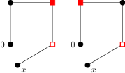
Figure 3: Diagrammatic representation of the bound used on $\widetilde{\psi}(p)$. There are three diagrams for the three possible configurations with two of the diagrams equal by symmetry. Each diagram is a path from $0$ to $x$ with three extra vertices, two of which (square and box) have the same torus projection but are distinct. For (6.2) we are interested only in the case $x=0$.

6.3 Higher-loop diagrams

To deal with $N\geq 2$, we define $P^{(N)}[0,n]$ and $Q^{(N)}[0,n]$ by

$$P^{(N)}[0,n] =\sum_{L\in\mathcal{L}^{(N)}[0,n]}\prod_{st\in L}(-U_{st})\Big{(}\prod_{s^{\prime}t^{\prime}\in\mathcal{C}(L)}(1+\beta U_{s^{\prime}t^{\prime}})-\prod_{s^{\prime}t^{\prime}\in\mathcal{C}(L)}(1+\beta U^{\mathbb{T}}_{s^{\prime}t^{\prime}})\Big{)},$$ (6.37)

$$Q^{(N)}[0,n] =\sum_{L\in\mathcal{L}^{(N)}[0,n]}\Big{(}\prod_{st\in L}(-U^{\mathbb{T}}_{st})-\prod_{st\in L}(-U_{st})\Big{)}\prod_{s^{\prime}t^{\prime}\in\mathcal{C}(L)}(1+\beta U^{\mathbb{T}}_{s^{\prime}t^{\prime}}).$$ (6.38)

By the formula for $\Delta^{(N)}(z)$ in (6.10),

$$\Delta^{(N)}(z)=\beta^{N}\sum_{n=2}^{\infty}z^{n}\sum_{\omega\in\mathcal{W}_{n}}\Big{(}Q^{(N)}[0,n]-P^{(N)}[0,n]\Big{)}.$$ (6.39)

It follows from $U_{st}^{\mathbb{T}}\leq U_{st}\leq 0$ that both $P^{(N)}[0,n]$ and $Q^{(N)}[0,n]$ are nonnegative. Then we define

$$S^{(N)}(z) =\beta^{N}\sum_{n=2}^{\infty}z^{n}\sum_{\omega\in\mathcal{W}_{n}}P^{(N)}[0,n],$$ (6.40)

$$T^{(N)}(z) =\beta^{N}\sum_{n=2}^{\infty}z^{n}\sum_{\omega\in\mathcal{W}_{n}}Q^{(N)}[0,n],$$ (6.41)

so that

$$\Delta^{(N)}(z) =T^{(N)}(z)-S^{(N)}(z).$$ (6.42)

Similarly,

$$\Delta^{\prime}(z) =\sum_{N=1}^{\infty}(-1)^{N+1}\Delta^{\prime(N)}(z),$$ (6.43)

with

$$\Delta^{\prime(N)}(z) =T^{\prime(N)}(z)-S^{\prime(N)}(z),$$ (6.44)

where

$$zS^{\prime(N)}(z) =\beta^{N}\sum_{n=2}^{\infty}nz^{n}\sum_{\omega\in\mathcal{W}_{n}}P^{(N)}[0,n],$$ (6.45)

$$zT^{\prime(N)}(z) =\beta^{N}\sum_{n=2}^{\infty}nz^{n}\sum_{\omega\in\mathcal{W}_{n}}Q^{(N)}[0,n].$$ (6.46)

We will prove the following proposition. For simplicity, we do not attempt to prove sharp bounds on $S^{N}$ and $S^{\prime(N)}$, although we believe that these terms are in fact smaller than $T^{N}$ and $T^{\prime(N)}$ (via improved decay in $V$, so not only smaller by an extra factor $\beta$). We again absorb any polynomial factors in $N$ into $C^{N}$ as discussed below (5.4).

Proposition 6.7.

Let $d>4$ and let $\beta>0$ be sufficiently small. Let $z\in U$ and let $N\geq 2$. There is a constant $C$ independent of $\beta,r,N,z$ such that

$$|S^{(N)}(z)| \leq\beta(C\beta)^{N}\frac{r^{2}+\chi(|z|)}{V},$$ (6.47)

$$|zS^{\prime(N)}(z)| \leq\beta(C\beta)^{N}\frac{\chi(|z|)(r^{2}+\chi(|z|))}{V},$$ (6.48)

$$|T^{(N)}(z)| \leq(C\beta)^{N}\frac{r^{2}+\chi(|z|)}{V},$$ (6.49)

$$|zT^{\prime(N)}(z)| \leq(C\beta)^{N}\frac{\chi(|z|)(r^{2}+\chi(|z|))}{V}.$$ (6.50)

Proof of Proposition 6.2.

For $N\geq 2$, this is a direct consequence of Proposition 6.7 together with (6.42) and (6.44). For $N=1$, it is an immediate corollary of Propositions 6.4 and 6.6. ∎

It remains only to prove Proposition 6.7.

6.4 Proof of Proposition 6.7

We begin with some initial bounds on $S^{(N)}$ and $T^{(N)}$ in Lemma 6.8. Although we need estimates for complex $z$, we see from (6.42) and from non-negativity of $P^{(N)}[0,n]$ and $Q^{(N)}[0,n]$ that for any complex $z$,

$$|\Delta^{(N)}(z)|\leq S^{(N)}(|z|)+T^{(N)}(|z|),$$ (6.51)

and similarly for $|\Delta^{{}^{\prime}(N)}(z)|$. For this reason, we will only be working with real non-negative $z$ in the rest of this section.

6.4.1 Bounds on $S,T$

Lemma 6.8.

For any $z\geq 0$ and $N\geq 2$, $T^{(N)}(z)$ and $S^{(N)}(z)$ are nonnegative and satisfy

$$S^{(N)}(z) \leq\beta^{N+1}\sum_{n=1}^{\infty}z^{n}\sum_{\omega\in\mathcal{W}_{n}}\sum_{L\in\mathcal{L}^{(N)}[0,n]}\sum_{ab\in\mathcal{C}(L)}(-U^{+}_{ab})\prod_{st\in L}(-U_{st})\prod_{s^{\prime}t^{\prime}\in\mathcal{C}(L)}(1+\beta U_{s^{\prime}t^{\prime}}),$$ (6.52)

$$T^{(N)}(z) \leq\beta^{N}\sum_{n=1}^{\infty}z^{n}\sum_{\omega\in\mathcal{W}_{n}}\sum_{L\in\mathcal{L}^{(N)}[0,n]}\sum_{ab\in L}(-U^{+}_{ab})\prod_{st\in L\setminus\{ab\}}(-U^{\mathbb{T}}_{st})\prod_{s^{\prime}t^{\prime}\in\mathcal{C}(L)}(1+\beta U^{\mathbb{T}}_{s^{\prime}t^{\prime}}).$$ (6.53)

In addition, $zS^{\prime(N)}(z)$ and $zT^{\prime(N)}(z)$ are bounded by the above right-hand sides with $z^{n}$ replaced by $nz^{n}$.

Proof.

Starting with $S^{(N)}(z)$, we note that it follows from (6.17) that

$$P^{(N)}[0,n] =\sum_{L\in\mathcal{L}^{(N)}[0,n]}\prod_{st\in L}(-U_{st})\prod_{s^{\prime}t^{\prime}\in\mathcal{C}(L)}(1+\beta U_{s^{\prime}t^{\prime}})\Big{(}1-\prod_{s^{\prime}t^{\prime}\in\mathcal{C}(L)}(1+\beta U^{+}_{s^{\prime}t^{\prime}})\Big{)}.$$ (6.54)

We then use (6.24) to see that

$$P^{(N)}[0,n] \leq\sum_{L\in\mathcal{L}^{(N)}[0,n]}\prod_{st\in L}(-U_{st})\prod_{s^{\prime}t^{\prime}\in\mathcal{C}(L)}(1+\beta U_{s^{\prime}t^{\prime}})\sum_{ab\in\mathcal{C}(L)}(-\beta U^{+}_{ab}).$$ (6.55)

Upon multiplying by $z^{n}$ and summing over $n$ this gives the bound on $S^{(N)}$.

For $T^{(N)}$, we use the identity $U_{st}=U_{st}^{\mathbb{T}}(1+U_{st}^{+})$ which is a consequence of the definitions (6.14)–(6.16), followed by (6.24), followed by the identity $U^{+}_{ab}U^{\mathbb{T}}_{ab}=U_{ab}^{+}$, to see that

$$\prod_{st\in L}(-U^{\mathbb{T}}_{st})-\prod_{st\in L}(-U_{st}) =\left[1-\prod_{st\in L}(1+U^{+}_{st})\right]\prod_{st\in L}(-U^{\mathbb{T}}_{st})$$

$$\leq\sum_{ab\in L}(-U_{ab}^{+})\prod_{st\in L}(-U^{\mathbb{T}}_{st})$$

$$=\sum_{ab\in L}(-U^{+}_{ab})\prod_{st\in L\setminus\{ab\}}(-U^{\mathbb{T}}_{st}).$$ (6.56)

With (6.38) and (6.41), this leads to (6.53).

For the derivatives it is the same, apart from the occurrence of $nz^{n}$ rather than $z^{n}$ due to differentiation. ∎

6.4.2 Proof of bounds on $T$

Proof of (6.49)–(6.50).

We are interested in nonnegative $z$ in the disk $U$ so we take $z\in[0,z_{c}(1-V^{-1/2})]$. We reinterpret the bound on $T^{(N)}$ in Lemma 6.8 in terms of a sum over torus walks. In this interpretation, we replace the sum over $\mathbb{Z}^{d}$-walks

$$\sum_{\omega\in\mathcal{W}_{n}}\sum_{L\in\mathcal{L}^{(N)}[0,n]}\sum_{ab\in L}(-U^{+}_{ab})\prod_{st\in L\setminus\{ab\}}(-U^{\mathbb{T}}_{st})\prod_{s^{\prime}t^{\prime}\in\mathcal{C}(L)}(1+\beta U^{\mathbb{T}}_{s^{\prime}t^{\prime}})$$ (6.57)

from (6.53) by a sum over torus walks

$$\sum_{\omega\in\mathcal{W}_{n}^{\mathbb{T}}}\sum_{L\in\mathcal{L}^{(N)}[0,n]}\sum_{ab\in L}(-U^{{\rm wrap}}_{ab})\prod_{st\in L\setminus\{ab\}}(-U_{st})\prod_{s^{\prime}t^{\prime}\in\mathcal{C}(L)}(1+\beta U_{s^{\prime}t^{\prime}}),$$ (6.58)

where $U^{{\rm wrap}}_{ab}$ is equal to $-1$ if $\omega(a)=\omega(b)$ via a path that wraps around the torus and otherwise is equal to zero. Then walks that make a nonzero contribution to (6.58) follow the trajectory of the familiar $N$-loop lace diagram (from Figure 2) on the torus with the restriction that at least one of the diagram loops must wrap around the torus as in Figure 4.

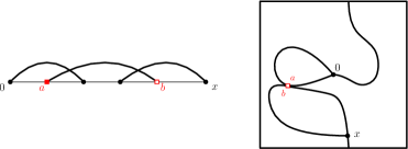
Figure 4: An example of a 3-bond lace with a corresponding torus walk configuration contributing to $T^{(3)}(z)$.

This wrapping loop consists of two (if it is one of the end loops) or three (if it is an interior loop) subwalks. One of these subwalks must have $\ell_{\infty}$-displacement at least $r/3$, because the loop travels a distance of at least $r$. We sum over the two or three cases which specify which of the subwalks must travel at least $r/3$. Once that subwalk is fixed, using Lemma 4.6 we bound its diagram line with the supremum norm, and bound all the other lines as usual by $\|G_{z}^{\mathbb{T}}\star G_{z}^{\mathbb{T}}\|_{\infty}^{N-1}$. The lift of the long subwalk to $\mathbb{Z}^{d}$ must have $\ell_{\infty}$-displacement at least $r/3$. It is therefore bounded above (using $K^{\mathbb{T}}\leq K$) by

$$\sup_{x\in\mathbb{T}_{r}^{d}}\sum_{u\in\mathbb{Z}^{d}:\|x+ru\|_{\infty}\geq r/3}G_{z}(x+ru).$$ (6.59)

If the torus point $x$ satisfies $\|x\|_{\infty}\geq r/3$ then we can simply remove the restriction on the sum over $u$ and bound the right-hand side using (3.36), by $G_{z}(x)+C\chi/V\prec r^{-(d-2)}+\chi/V$. If instead $\|x\|_{\infty}<r/3$, then the $u=0$ term is excluded by the restriction on the summation, and we instead have a bound just by $\chi/V$ as in (3.39). Thus, in any case, we obtain a factor

$$\frac{1}{V}(r^{2}+\chi(z))$$ (6.60)

from the long line, so as in (4.22) we obtain

$$T^{(N)}(z) \leq\beta^{N}O(N)\left(\frac{r^{2}+\chi(z)}{V}\right)\|G_{z}^{\mathbb{T}}\star G_{z}^{\mathbb{T}}\|_{\infty}^{N-1}$$ (6.61)

and the desired estimate (6.49) follows from (3.37).

For the derivative, we can proceed as above but now with an extra vertex. If the extra vertex is on the long line identified as above then we replace $G_{z}^{\mathbb{T}}(x)$ in the above by $(G_{z}^{\mathbb{T}}\star G_{z}^{\mathbb{T}})(x)$ (this is as in (5.3)) with the restriction that one of the two-point functions in the convolution must have a lift whose displacement is of order $r$. We bound the supremum norm of this restricted convolution by putting the $\ell_{\infty}$-norm on the long factor and the $\ell_{1}$-norm (which yields $\chi^{\mathbb{T}}\leq\chi$) on the other. The $\ell_{\infty}$ norm is bounded exactly as in the previous paragraph, so that overall we obtain a bound this line by

$$\frac{1}{V}(r^{2}+\chi)\chi.$$ (6.62)

If the extra vertex is not on the long line then we replace the usual weight $G_{z}^{\mathbb{T}}$ for the line containing the extra vertex by $G_{z}^{\mathbb{T}}\star G_{z}^{\mathbb{T}}$ so that one factor $\|G_{z}^{\mathbb{T}}\star G_{z}^{\mathbb{T}}\|_{\infty}$ gets replaced by $\|G_{z}^{\mathbb{T}}\star G_{z}^{\mathbb{T}}\star G_{z}^{\mathbb{T}}\|_{\infty}$. This gives, as in Proposition 4.7,

$$T^{\prime(N)}(z) \leq\beta^{N}O(N)\left(\frac{r^{2}\chi(z)+\chi(z)^{2}}{V}\right)\|G_{z}^{\mathbb{T}}\star G_{z}^{\mathbb{T}}\|_{\infty}^{N-1}$$

$$\quad+\beta^{N}O(N)\left(\frac{r^{2}+\chi(z)}{V}\right)\|G_{z}^{\mathbb{T}}\star G_{z}^{\mathbb{T}}\star G_{z}^{\mathbb{T}}\|_{\infty}\|G_{z}^{\mathbb{T}}\star G_{z}^{\mathbb{T}}\|_{\infty}^{N-2}.$$ (6.63)

The first term has the upper bound that we desire. By (3.38) and (3.29), the three-fold convolution is less than $\chi+\chi^{3}/V$, so overall the second term contains a factor

$$\frac{\chi(z)(r^{2}+\chi(z))}{V}\left(1+\frac{\chi(z)^{2}}{V}\right).$$ (6.64)

By Remark 6.3, this is sufficient. ∎

6.4.3 Proof of bounds on $S$

We now prove the bounds on $S^{(N)}$ and $S^{\prime(N)}$ stated in (6.47)–(6.48). This is the most elaborate part of the proof of Proposition 6.1. Recall from (6.52) that

$$S^{(N)}(z) \leq\beta^{N+1}\sum_{n=1}^{\infty}z^{n}\sum_{\omega\in\mathcal{W}_{n}}\sum_{L\in\mathcal{L}^{(N)}[0,n]}\sum_{ab\in\mathcal{C}(L)}(-U^{+}_{ab})\prod_{st\in L}(-U_{st})\prod_{s^{\prime}t^{\prime}\in\mathcal{C}(L)}(1+\beta U_{s^{\prime}t^{\prime}}).$$ (6.65)

This contains the desired factor $\beta^{N+1}$ in $S^{(N)}$ which we do not carry through the rest of the analysis.

For fixed $\omega$ and $L$,

$$\sum_{ab\in\mathcal{C}(L)}(-U^{+}_{ab})(\omega) =\sum_{x\in\mathbb{Z}^{d}}\sum_{u\neq 0}\sum_{ab\in\mathcal{C}(L)}\mathbbm{1}\{\omega(a)=x,\;\omega(b)=x+ru\}.$$ (6.66)

Thus, the diagram corresponding to $S^{(N)}$ is a standard $\Pi$-diagram (as in Figure 2) with two additional vertices $x$ and $x+ru$ that are distinct but have the same torus projection. In the $N$-loop diagram, we label the $2N-1$ subwalks from $1$ to $2N-1$ in their order of appearance. From the definition of compatible edges and from Figure 5, we see that the additional two vertices must belong to two subwalks whose labels differ by at most $3$ or are identical. In what follows, for simplicity we restrict attention to the case where the vertices $a,b$ in Figure 5 do not lie on the lines $1,2,2N-2$ or $2N-1$, i.e. on the first or last loop. The omitted extreme cases are straightforward extensions of our analysis.

We fix $z\in[0,z_{c}(1-V^{-1/2})]$ for the rest of this section. We will prove the inequalities listed in the following three cases. Together, they provide a proof of Proposition 6.7 and in fact most of these bounds are better than what is needed.

Case 1: $a,b$ occur on the same subwalk: $b=b_{1},b^{\prime}_{1}$ in Figure 6. We prove that

$$\text{ Case~{}1(a): }S^{(N)}(z)\prec C^{N}\frac{r^{2}}{V},\qquad\text{ Case~{}1(b): }S^{\prime(N)}(z)\prec C^{N}\frac{\chi(z)(r^{2}+\chi(z))}{V}.$$ (6.67)

Case 2: $a,b$ occur on the same loop but on different subwalks: $b=b_{2},b_{3},b^{\prime}_{2},b^{\prime}_{3},b^{\prime}_{4},b^{\prime}_{5}$ in Figure 6. We prove that

$$\text{ Case~{}2(a): }S^{(N)}(z)\prec C^{N}\frac{\chi(z)}{V}\frac{1}{r^{d-4}},\qquad\text{ Case~{}2(b): }S^{\prime(N)}(z)\prec C^{N}\frac{\chi(z)^{2}}{V}\frac{1}{r^{(d-4)/2}}.$$ (6.68)

Case 3: $a,b$ occur on adjacent loops: $b=b_{4},b_{5},b_{6},b^{\prime}_{6}$ in Figure 6. We prove that

$$\text{ Case~{}3(a): }S^{(N)}(z)\prec C^{N}\frac{\chi(z)}{V}\frac{1}{r^{d-4}},\qquad\text{ Case~{}3(b): }S^{\prime(N)}(z)\prec C^{N}\frac{\chi(z)}{V}\frac{1}{r^{(d-4)/2}}.$$ (6.69)

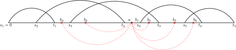
Figure 5: A $5$-edge lace with compatible edges for $a$ depicted with dotted lines: there are $6$ subwalks where $b$ may occur, with generic locations denoted $b_{1},\ldots,b_{6}$.

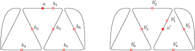
Figure 6: Walk diagrams for the lace in Figure 5 with possible locations for the vertices $x$ and $x+ru$ from (6.66) represented by squares and boxes. Two possible configurations are depicted.

Case 1(a) for $S^{(N)}$. In this case, using Lemma 4.6 we bound the line containing $a,b$ with the supremum norm and bound all other lines with the bubble. We obtain $C^{N-1}$ times

$$\sup_{x\in\mathbb{Z}^{d}}\sum_{v\in\mathbb{Z}^{d}}\sum_{u\neq 0}G_{z}(v)G_{z}(ru)G_{z}(x-v-ru),$$ (6.70)

and we now focus on bounding (6.70). Since $u\neq 0$ we have $G_{z}(ru)\prec r^{-(d-2)}$. This gives an upper bound, up to multiplicative constant, of the form

$$r^{-(d-2)}\sup_{x\in\mathbb{Z}^{d}}\sum_{v\in\mathbb{Z}^{d}}\sum_{u\neq 0}G_{z}(v)G_{z}(x-v-ru)=r^{-(d-2)}\sup_{x\in\mathbb{Z}^{d}}\sum_{u\neq 0}{\sf B}_{z}(x-ru).$$ (6.71)

By (3.41) and the fact that ${\sf B}(y)$ is maximal at $y=0$ by the Cauchy–Schwarz inequality, this is bounded by

$$\frac{1}{r^{d-2}}\Big{(}{\sf B}_{z}(0)+C\frac{\chi(z)}{V}\Big{)},$$ (6.72)

from which we see that

Case 1(a) $$\prec C^{N}\frac{r^{2}}{V}\Big{(}1+\frac{\chi(z)^{2}}{V}\Big{)}.$$ (6.73)

By Remark 6.3, this is sufficient. ∎

Case 1(b) for $S^{\prime(N)}$. If the extra vertex from the derivative is on a different line than the one containing $a,b$, then we replace one factor $\|G_{z}*G_{z}\|_{\infty}$ by $\|G_{z}*G_{z}*G_{z}\|_{\infty}$, which by (3.29) is at most $\chi(z)$. This increases the bound from Case 1(a) by a factor $\chi$, leading to an overall bound from this contribution of the form

$$C^{N}\frac{r^{2}\chi(z)}{V}\Big{(}1+\frac{\chi(z)^{2}}{V}\Big{)}.$$ (6.74)

If the extra vertex is instead on the same line as $a,b$ then we bound that line as in the bound on $\widetilde{\psi}$ (recall Figure 3) in the proof of Proposition 6.6 with a multiple of the supremum over $x\in\mathbb{Z}^{d}$ of

$$\sum_{u\neq 0}\Big{(}{\sf B}_{z}(x-ru){\sf B}_{z}(ru)+{\sf T}_{z}(x-ru)G_{z}(ru)\Big{)}.$$ (6.75)

To see in detail how one of these terms arises, the first diagram of Figure 3 with the origin moved to the box represents

$$\sum_{u\neq 0}G_{z}(ru)\sum_{v,w\in\mathbb{Z}^{d}}G_{z}(v)G_{z}(w-v)G_{z}(w+x-ru)=\sum_{u\neq 0}G_{z}(ru){\sf T}_{z}(x-ru).$$ (6.76)

The sum (6.75) is shown in Lemma 6.5 to be bounded by $V^{-1}\chi(z)^{2}$ uniformly over $x\in\mathbb{Z}^{d}$. Finally, summing both cases gives

$$\text{ Case~{}1(b)}\prec C^{N}\frac{\chi(z)^{2}}{V}+C^{N}\frac{r^{2}\chi(z)}{V}\Big{(}1+\frac{\chi(z)^{2}}{V}\Big{)}.$$ (6.77)

This is sufficient by Remark 6.3. ∎

For Cases 2 and 3, we isolate some useful estimates in Lemma 6.9. For this, we define functions $\Psi_{z}$ and $\widetilde{\Psi}_{z}$ on $\mathbb{Z}^{d}$ by

$$\Psi_{z}(x) =\Big{[}\sum_{u\neq 0}(G_{z}^{2}*G_{z}^{2})(x+ru)\Big{]}^{1/2},$$ (6.78)

$$\widetilde{\Psi}_{z}(x) =\Big{[}\sum_{u\neq 0}\left((G_{z}*G_{z})^{2}*G_{z}^{2}\right)(x+ru)\Big{]}^{1/2}.$$ (6.79)

Lemma 6.9.

Let $d>4$ and let $\beta>0$ be sufficiently small. For any $z<z_{c}$,

$$\Psi_{z}(0) \prec\frac{1}{r^{d-2}},\qquad\|\Psi_{z}G_{z}\|_{2}\prec\frac{1}{r^{d-2}},$$ (6.80)

$$\widetilde{\Psi}_{z}(0) \prec\frac{\chi(z)}{V^{1/2}},\qquad\|\widetilde{\Psi}_{z}G_{z}\|_{2}\prec\frac{\chi(z)}{V^{1/2}},$$ (6.81)

and these bounds remain satisfied with any $G_{z}$ (including those in $\Psi_{z}$ and $\widetilde{\Psi}_{z}$) replaced by $(G_{z}^{2}*G_{z}^{2})^{1/2}$.

Proof.

By the first case of Lemma 3.3, $(G_{z}^{2}*G_{z}^{2})(x)\prec\langle x\rangle^{-(2d-4)}e^{-2c_{1}m(z)\|x\|_{\infty}}$, so by Lemma 3.4 with $a=4-d<0$ and $x=0\in\mathbb{T}_{r}^{d}$ we obtain the desired bound $\Psi_{z}(0)^{2}\prec r^{-(2d-4)}$. Similarly, $[(G_{z}*G_{z})^{2}*G_{z}^{2}](x)\prec\langle x\rangle^{-(2d-8)}e^{-2c_{1}m(z)\|x\|_{\infty}}$ and from Lemma 3.4 with $a=8-d$ we obtain the desired estimate

$$\widetilde{\Psi}_{z}(0)^{2}\prec\sum_{u\neq 0}\frac{e^{-2c_{1}m(z)\|ru\|_{\infty}}}{\langle ru\rangle^{2d-8}}\prec\frac{\chi(z)^{2}}{V},$$ (6.82)

where we have chosen the last bound so as to accommodate the worst case which is $d\downarrow 4$.

For the $\ell_{2}$ bounds, we first use the definition of $\Psi_{z}$ to see that

$$\|\Psi_{z}G_{z}\|_{2}^{2} =\sum_{u\neq 0}\sum_{x}G_{z}(x)^{2}(G_{z}^{2}*G_{z}^{2})(x+ru)=\sum_{u\neq 0}(G_{z}^{2}*G_{z}^{2}*G_{z}^{2})(ru).$$ (6.83)

By Lemma 3.3, $(G_{z}^{2}*G_{z}^{2}*G_{z}^{2})$ obeys the same estimate as $G_{z}^{2}*G_{z}^{2}$ used in the previous paragraph to bound $\Psi_{z}(0)$, so (6.83) is also bounded by $r^{-(2d-4)}$, as required. Similarly,

$$\|\widetilde{\Psi}_{z}G_{z}\|_{2}^{2} =\sum_{u\neq 0}((G_{z}*G_{z})^{2}*G_{z}^{2}*G_{z}^{2})(ru),$$ (6.84)

and the extra factor $G_{z}^{2}$ in the convolution, compared to the bound on $\widetilde{\Psi}_{z}(0)$, again has no effect and we again obtain an upper bound $V^{-1}\chi(z)^{2}$ as in (6.82).

Finally, by Lemma 3.3 and since $2d-4>d$,

$$(G_{z}^{2}*G_{z}^{2})^{1/2}(x)\prec\frac{e^{-c_{1}m(z)\|x\|_{\infty}}}{\langle x\rangle^{d-2}},$$ (6.85)

which is the same as the bound on $G_{z}$ that we have used throughout this proof. Therefore the above discussion also applies when we replace any $G_{z}$ by $(G_{z}^{2}*G_{z}^{2})^{1/2}$. ∎

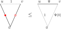
Figure 7: Diagrammatic bound for Case 2(a). Lines other than $G_{z}$ lines have their associated weights written next to them. Lines with constant weights are dotted.

Case 2(a) for $S^{(N)}$. We place the origin at the single common endpoint of the two distinct subwalks containing $a$ and $b$, as in Figure 7. The portion of the diagram corresponding to these two lines is

$$\sum_{x\in\mathbb{Z}^{d}}\sum_{s\neq 0}G_{z}(x)G_{z}(u-x)G_{z}(x+rs)G_{z}(v-x-rs).$$ (6.86)

We reorganise the above sum and apply the Cauchy–Schwarz inequality to see that it is bounded by

$$\sum_{s\neq 0}\sum_{x\in\mathbb{Z}^{d}}\left(G_{z}(x)G_{z}(x+rs)\right)\left(G_{z}(u-x)G_{z}(v-x-rs)\right)$$

$$\quad\leq\Big{(}\sum_{s\neq 0}(G_{z}^{2}*G_{z}^{2})(rs)\Big{)}^{1/2}\Big{(}\sum_{s\neq 0}(G_{z}^{2}*G_{z}^{2})(v-u+rs)\Big{)}^{1/2}=\Psi_{z}(0)\Psi_{z}(v-u).$$ (6.87)

We interpret this inequality as an upper bound in which the weights of the original diagram lines containing $a$ and $b$ are replaced by constant functions $1$ and $\Psi_{z}(0)$, and the weight of the line joining $u$ and $v$ is replaced by $\Psi_{z}G_{z}$ (instead of the original $G_{z}$). This is depicted in Figure 7.

We bound this new diagram using Lemma 4.6. We place the supremum norm on the line containing $\Psi_{z}(0)$. There is one factor with lines $G_{z}$ and $1$ which is dominated by $\|G_{z}*1\|_{\infty}$. Another factor with lines $G_{z}$ and $\Psi_{z}G_{z}$ is controlled by $\|(\Psi_{z}G_{z})*G_{z}\|_{\infty}$ All the other factors have $G_{z}$ lines and give standard factors involving $G_{z}*G_{z}$ as usual. By combining the above contributions, for $N\geq 3$ we obtain the upper bound

$$\|G_{z}*G_{z}\|_{\infty}^{N-3}\|G_{z}*1\|_{\infty}\|(\Psi_{z}G_{z})*G_{z}\|_{\infty}\|\Psi_{z}(0)\|_{\infty}.$$ (6.88)

By using Cauchy–Schwarz for the first and third factors and rewriting the second and fourth ones we can simplify the bound as

$$\|G_{z}\|_{2}^{2N-5}\,\|G_{z}\|_{1}\,\|\Psi_{z}G_{z}\|_{2}\,\Psi_{z}(0).$$ (6.89)

Since $\|G_{z}\|_{1}=\chi(z)$ and $\|G_{z}\|_{2}\leq\|G_{z_{c}}\|_{2}<\infty$, it follows from Lemma 6.9 that (6.89) is bounded above by

$$\text{ Case~{}2(a)}\prec C^{N}\chi(z)\frac{1}{r^{d-2}}\frac{1}{r^{d-2}}=C^{N}\frac{\chi(z)}{V}\frac{1}{r^{d-4}}.$$ (6.90)

This gives the claimed result. ∎

Case 2(b) for $S^{\prime(N)}$. The derivative adds a vertex to the diagrams arising in Case 2(a). This amounts to replacing exactly one of the weights $G_{z}$ by $G_{z}*G_{z}$. We thus obtain an upper bound by adapting the proof of Case 2(a) by replacing exactly one of the $G_{z}$ factors in (6.89) (including the ones in $\Psi_{z}$) by $G_{z}*G_{z}$. Note that $\widetilde{\Psi}_{z}$ is exactly obtained from $\Psi_{z}$ by replacing one of its $G_{z}$ factors by $G_{z}*G_{z}$. This leads to one of the new factors, compared to (6.89),

$$\|G_{z}*G_{z}\|_{2} \leq\chi(z),\qquad\|G_{z}*G_{z}\|_{1}=\chi(z)^{2},$$ (6.91)

$$\|\widetilde{\Psi}_{z}G_{z}\|_{2}=\|\Psi_{z}(G_{z}*G_{z})\|_{2} \leq\frac{\chi(z)}{V^{1/2}},\qquad\widetilde{\Psi}_{z}(0)\leq\frac{\chi(z)}{V^{1/2}}.$$ (6.92)

The first inequality follows as usual from Lemma 3.4 and is sharp when $d\downarrow 4$, the second is an elementary identity, and the third and fourth follow from Lemma 6.9 together with the identity $\|\widetilde{\Psi}_{z}G_{z}\|_{2}=\|\Psi_{z}(G_{z}*G_{z})\|_{2}$ (which holds by definition). The net effect on (6.90) is to replace a factor $r^{-(d-2)}$ by $V^{-1/2}\chi$ or to multiply by an additional factor $\chi$. Since $r^{d-2}V^{-1/2}>1$, the former replacement dominates and we conclude that

$$\text{ Case~{}2(b)}\prec C^{N}\chi(z)\frac{1}{r^{d-2}}\frac{\chi(z)}{r^{d/2}}=C^{N}\frac{\chi(z)^{2}}{V}\frac{1}{r^{(d-4)/2}}.$$ (6.93)

∎

Case 3(a) for $S^{(N)}$. Consider first the case where the lines containing $a$ and $b$ have no common endpoint (which can occur only for $N\geq 4$), as in Figure 8. These two lines involve four $G_{z}$ factors and by the Cauchy–Schwarz inequality their contribution obeys

$$\sum_{x\in\mathbb{Z}^{d}}\sum_{s\neq 0}(G_{z}(v-x)G_{z}(w-x-rs))(G_{z}(x-u)G_{z}(x+rs)) \leq\Psi_{z}(w-v)\Psi_{z}(u).$$ (6.94)

This amounts to replacing each of the two opposite lines of a pair of consecutive loops by $\Psi_{z}G_{z}$ instead of $G_{z}$, and the other pair of lines by $1$, as in Figure 8. We bound this new diagram using Lemma 4.6: we place the supremum norm on one of the $1$ lines and extract the rest of the line pairs. Two pairs have $\Psi_{z}G_{z}$ and $G_{z}$ instead of a single pair as in Case 2(a), and there is also one pair with $G_{z}$ and $1$. The rest are standard pairs with $G_{z}$ lines. This gives an overall upper bound

$$\|G_{z}*G_{z}\|_{\infty}^{N-4}\|G_{z}*1\|_{\infty}\|(\Psi_{z}G_{z})*G_{z}\|_{\infty}^{2}\|1\|_{\infty}.$$ (6.95)

By Lemma 6.9, we obtain an upper bound on this case by

$$\|G_{z}\|_{2}^{2N-6}\|G_{z}\|_{1}\|\Psi_{z}G_{z}\|_{2}^{2}\leq C^{N}\chi(z)\frac{1}{r^{2(d-2)}}=C^{N}\frac{\chi(z)}{V}\frac{1}{r^{d-4}}.$$ (6.96)

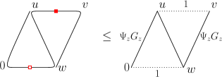
Figure 8: Schematic representation of the bound used for the first case of Case 3(a). Lines with constant weights are dotted.

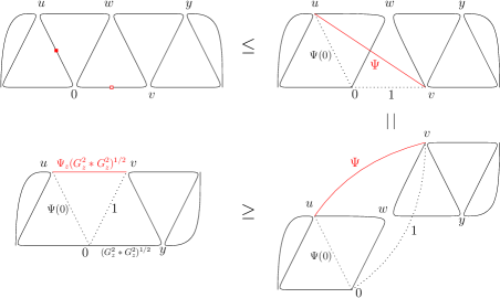
Figure 9: Schematic representation of the bound used for the second case of Case 3(a). We use the Cauchy–Schwarz inequality twice. The line between $u$ and $v$ is first non-existent (or equivalently constant equal to $1$) then $\Psi$ and finally $\Psi(G^{2}*G^{2})^{1/2}$. Lines with constant weights are dotted.

If instead the two lines containing $a$ and $b$ share an endpoint, then we place the origin of the diagram at this vertex and apply the Cauchy–Schwarz inequality exactly as in (6.4.3). This does not give a standard diagram, due to the atypical diagonal $\Psi$ line in Figure 9. To deal with this, we apply the Cauchy–Schwarz inequality a second time, to the portion of the diagram with this diagonal line where the sum runs over the one vertex in the two loops that does not belong to either of the two lines ($w$ in Figure 9). This gives

$$\sum_{w}[G_{z}(w)G_{z}(y-w)][G_{z}(v-w)G_{z}(u-w)] \leq(G_{z}^{2}*G_{z}^{2})^{1/2}(v-u)(G_{z}^{2}*G_{z}^{2})^{1/2}(y).$$ (6.97)

Diagrammatically, as illustrated in Figure 9, this has the effect of removing a loop to produce the diagram for Case 2(a) for $S^{(N-1)}$ (with slightly modified weights) instead of $S^{(N)}$. Since our estimates apply also when $G_{z}$ is replaced by $(G_{z}^{2}*G_{z}^{2})^{1/2}$ (recall Lemma 6.9), we therefore again obtain a bound $C^{N}V^{-1}\chi(z)r^{-(d-4)}$ as in (6.90). Both contributions in Case 3(a) are equal and the overall bound is thus

$$\text{ Case~{}3(a)}\prec C^{N}\frac{\chi(z)}{V}\frac{1}{r^{d-4}},$$ (6.98)

which is sufficient. ∎

Case 3(b) for $S^{\prime(N)}$. As in Case 2(b), the derivative effectively replaces exactly one of the weights $G_{z}$ encountered in Case 3(a) by $G_{z}*G_{z}$. We use the estimates obtained in (6.91)-(6.92). The only difference comes from the second application of the Cauchy–Schwarz inequality in (6.97) which changes some $G_{z}$ factors to $(G^{2}_{z}*G^{2}_{z})^{1/2}$. However, since both functions are bounded in the same way (as in Lemma 6.9) this leads again to an overall bound

$$\text{ Case~{}3(b)}\prec C^{N}\frac{\chi(z)^{2}}{V}\frac{1}{r^{(d-4)/2}}.$$ (6.99)

This completes the proof. ∎

References

- [1] L. Avena, E. Bolthausen, and C. Ritzmann. A local CLT for convolution equations with an application to weakly self-avoiding walks. Ann. Probab., 44:206–234, (2016).
- [2] R. Bauerschmidt, D.C. Brydges, and G. Slade. Logarithmic correction for the susceptibility of the 4-dimensional weakly self-avoiding walk: a renormalisation group analysis. Commun. Math. Phys., 337:817–877, (2015).
- [3] C. Borgs, J.T. Chayes, R. van der Hofstad, G. Slade, and J. Spencer. Random subgraphs of finite graphs: I. The scaling window under the triangle condition. Random Struct. Alg., 27:137–184, (2005).
- [4] M. Bousquet-Mélou, A.J. Guttmann, and I. Jensen. Self-avoiding walks crossing a square. J. Phys. A: Math. Gen., 38:9158–9181, (2005).
- [5] D.C. Brydges, T. Helmuth, and M. Holmes. The continuous-time lace expansion. Commun. Pure Appl. Math., 74:2251–2309, (2021).
- [6] D.C. Brydges and T. Spencer. Self-avoiding walk in 5 or more dimensions. Commun. Math. Phys., 97:125–148, (1985).
- [7] F. Camia, J. Jiang, and C.M. Newman. The effect of free boundary conditions on the Ising model in high dimensions. Probab. Theory Related Fields, 181:311–328, (2021).
- [8] N. Clisby. Scale-free Monte Carlo method for calculating the critical exponent of self-avoiding walks. J. Phys. A: Math. Theor., 50:264003, (2017).
- [9] Y. Deng, T.M. Garoni, J. Grimm, A. Nasrawi, and Z. Zhou. The length of self-avoiding walks on the complete graph. J. Stat. Mech: Theory Exp., 103206, (2019).
- [10] Y. Deng, T.M. Garoni, J. Grimm, and Z. Zhou. Unwrapped two-point functions on high-dimensional tori. J. Stat. Mech: Theory Exp., 053208, (2022).
- [11] E. Derbez and G. Slade. The scaling limit of lattice trees in high dimensions. Commun. Math. Phys., 193:69–104, (1998).
- [12] C. Domb and G.S. Joyce. Cluster expansion for a polymer chain. J. Phys. C: Solid State Phys., 5:956–976, (1972).
- [13] H. Duminil-Copin, S. Ganguly, A. Hammond, and I. Manolescu. Bounding the number of self-avoiding walks: Hammersley–Welsh with polygon insertion. Ann. Probab., 48:1644–1692, (2020).
- [14] H. Duminil-Copin and A. Hammond. Self-avoiding walk is sub-ballistic. Commun. Math. Phys., 324:401–423, (2013).
- [15] H. Duminil-Copin, G. Kozma, and A. Yadin. Supercritical self-avoiding walks are space-filling. Ann. Inst. H. Poincaré Probab. Statist., 50:315–326, (2014).
- [16] S. Golowich and J.Z. Imbrie. A new approach to the long-time behavior of self-avoiding random walks. Ann. Phys., 217:142–169, (1992).
- [17] S.E. Golowich and J.Z. Imbrie. The broken supersymmetry phase of a self-avoiding random walk. Commun. Math. Phys., 168:265–319, (1995).
- [18] A.J. Guttmann and I. Jensen. Self-avoiding walks and polygons crossing a domain on the square and hexagonal lattices. Preprint, https://arxiv.org/pdf/arXiv:2208.06744, (2022).
- [19] J.M. Hammersley and D.J.A. Welsh. Further results on the rate of convergence to the connective constant of the hypercubical lattice. Quart. J. Math. Oxford, (2), 13:108–110, (1962).
- [20] T. Hara. Decay of correlations in nearest-neighbor self-avoiding walk, percolation, lattice trees and animals. Ann. Probab., 36:530–593, (2008).
- [21] T. Hara, R. van der Hofstad, and G. Slade. Critical two-point functions and the lace expansion for spread-out high-dimensional percolation and related models. Ann. Probab., 31:349–408, (2003).
- [22] T. Hara and G. Slade. Self-avoiding walk in five or more dimensions. I. The critical behaviour. Commun. Math. Phys., 147:101–136, (1992).
- [23] M. Heydenreich and R. van der Hofstad. Random graph asymptotics on high-dimensional tori II: volume, diameter and mixing time. Probab. Theory Related Fields, 149:397–415, (2011). Correction: Probab. Theory Related Fields, 175:1183–1185, (2019).
- [24] M. Heydenreich and R. van der Hofstad. Progress in High-Dimensional Percolation and Random Graphs. Springer International Publishing Switzerland, (2017).
- [25] R. van der Hofstad, F. den Hollander, and G. Slade. A new inductive approach to the lace expansion for self-avoiding walks. Probab. Theory Related Fields, 111:253–286, (1998).
- [26] T. Hutchcroft. The Hammersley–Welsh bound for self-avoiding walk revisited. Electron. Commun. Probab., 23:Paper 5, (2018).
- [27] T. Hutchcroft. Self-avoiding walk on nonunimodular transitive graphs. Ann. Probab., 47:2801–2829, (2019).
- [28] T. Hutchcroft, E. Michta, and G. Slade. High-dimensional near-critical percolation and the torus plateau. Preprint, https://arxiv.org/pdf/2107.12971, (2021).
- [29] H. Kesten. On the number of self-avoiding walks. II. J. Math. Phys., 5:1128–1137, (1964).
- [30] K.M. Khanin, J.L. Lebowitz, A.E. Mazel, and Ya.G. Sinai. Self-avoiding walks in five or more dimensions: polymer expansion approach. Russian Math. Surveys, 50:403–434, (1995).
- [31] G.F. Lawler, O. Schramm, and W. Werner. On the scaling limit of planar self-avoiding walk. Proc. Symposia Pure Math., 72:339–364, (2004).
- [32] P.H. Lundow and K. Markström. The scaling window of the D Ising model with free boundary conditions. Nucl. Phys. B, 911:163–172, (2016).
- [33] N. Madras and G. Slade. The Self-Avoiding Walk. Birkhäuser, Boston, (1993).
- [34] E. Michta. The scaling limit of the weakly self-avoiding walk on a high-dimensional torus. Preprint, https://arxiv.org/pdf/2203.07695, (2022).
- [35] E. Michta, J. Park, and G. Slade. Universal finite-size scaling for the -dimensional multi-component hierarchical model. In preparation.
- [36] B. Nienhuis. Exact critical exponents of the models in two dimensions. Phys. Rev. Lett., 49:1062–1065, (1982).
- [37] V. Papathanakos. Finite-Size Effects in High-Dimensional Statistical Mechanical Systems: The Ising Model with Periodic Boundary Conditions. PhD thesis, Princeton University, (2006).
- [38] G. Slade. The Lace Expansion and its Applications. Springer, Berlin, (2006). Lecture Notes in Mathematics Vol. 1879. Ecole d’Eté de Probabilités de Saint–Flour XXXIV–2004.
- [39] G. Slade. The near-critical two-point function and the torus plateau for weakly self-avoiding walk in high dimensions. Preprint, https://arxiv.org/pdf/2008.00080, (2020).
- [40] G. Slade. Self-avoiding walk on the complete graph. J. Math. Soc. Japan, 72:1189–1200, (2020).
- [41] G. Slade. Self-avoiding walk on the hypercube. To appear in Random Structures Algorithms, https://arxiv.org/pdf/2108.03682, (2021).
- [42] G. Slade. A simple convergence proof for the lace expansion. Ann. I. Henri Poincaré Probab. Statist., 58:26–33, (2022).
- [43] M. Wittmann and A.P. Young. Finite-size scaling above the upper critical dimension. Phys. Rev. E, 90:062137, (2014).
- [44] A. Yadin. Self-avoiding walks on finite graphs of large girth. ALEA, Lat. Am. J. Probab. Math. Stat., 13:521–544, (2016).
- [45] Z. Zhou, J. Grimm, S. Fang, Y. Deng, and T.M. Garoni. Random-length random walks and finite-size scaling in high dimensions. Phys. Rev. Lett., 121:185701, (2018).