Complementarity relations for design-structured POVMs in terms of generalized entropies of order $\alpha\in(0,2)$

Abstract

Information entropies give a genuine way to characterize quantitatively an incompatibility in quantum measurements. Together with the Shannon entropy, few families of parametrized entropies have found use in various questions. It is also known that a possibility to vary the parameter can often provide more restrictions on elements of probability distributions. In quantum information processing, one often deals with measurements having some special structure. Quantum designs are currently the subject of active research, whence the aim to formulate complementarity relations for related measurements occurs. Using generalized entropies of order $\alpha\in(0,2)$, we obtain uncertainty and certainty relations for POVMs assigned to a quantum design. The structure of quantum designs leads to several restrictions on generated probabilities. We show how to convert these restrictions into two-sided entropic estimates. One of the used ways is based on truncated expansions of the Taylor type. The recently found method to get two-sided entropic estimates uses polynomials with flexible coefficients. We illustrate the utility of this method with respect to both the Rényi and Tsallis entropies. Possible applications of the derived complementarity relations are briefly discussed.

I Introduction

The Heisenberg uncertainty principle heisenberg is now interpreted as a scientific concept of general applicability. Quantum-mechanical complementarity relations are interesting not only as a reflection of principal features of the quantum world. They play a certain role in building feasible schemes for some tasks of quantum information, for instance, for entanglement detection, quantum tomography and steering. There exist several ways to characterize quantitatively potential uncertainties in various quantum measurements. The traditional approach to preparation uncertainty relations deals with the product of variances kennard ; robert . It has later been criticized for several reasons deutsch ; maass . Entropic relations have been proposed as a proper way to characterize quantum uncertainties. For finite-dimensional observables, basic results in this area are resumed in ww10 ; cbtw17 . Entropic uncertainty relations for continuous variables are reviewed in brud11 ; cerf19 .

Special types of measurements are widely used in quantum information science. Mutually unbiased bases bz10 and symmetric informationally complete measurements rbksc04 are especially important examples. They are linked to rather difficult questions about discrete structures in Hilbert space (see, e.g., the reviews fhs2017 ; fivo20 and references therein). Quantum and unitary designs are considered as a useful tool in quantum information processing ambain07 ; gross07 ; scottjpa8 ; dcel9 ; roy09 ; cirac18 ; bhmn19 ; kwg19 ; chart19 . Formally, quantum design is a complex projective $t$-design scottjpa . To the given quantum designs, we can assign one or several measurements with many restriction on generated probabilities. For such measurements, uncertainty relations in terms of $\alpha$-entropies of order $\alpha\geq 2$ were obtained in guhne20 ; rastdes . The question of deriving Shannon-entropy complementarity relations for design-structured POVMs was recently examined in rastpol and applied to quantum coherence in rastunc .

For integer values $\alpha\geq 2$, uncertainty relations directly follow from properties of quantum designs. The paper rastpol uses truncated expansions of the Taylor type and polynomials with flexible coefficients. The latter has been motivated by Lanczos lanczos as a good method to get oscillating approximations. As was shown in rastpol , polynomials with flexible coefficients also lead to fitting the function of interest from below or above solely. The aim of this work is to study the question, whether this method is suitable for generalized entropies. The paper is organized as follows. In Section II, the required material on quantum designs is given. In Section III, we derive two-sided estimates on a power function naturally connected with the considered entropies. In Section IV, complementarity relations for design-structured POVMs in terms of generalized entropies are formulated. Several applications of the derived relations are briefly discussed in Section V. In Section VI, we conclude the paper. Appendix A summarized auxiliary material.

II Preliminaries

In this section, we recall some facts about quantum designs. In $d$-dimensional Hilbert space ${\mathcal{H}}$, we consider lines passing through the origin. These lines form a complex projective space scottjpa . Up to a phase factor, each line is represented by a unit vector $|\phi\rangle\in{\mathcal{H}}$. The set ${\mathbb{D}}=\bigl{\{}|\phi_{k}\rangle:\,\langle\phi_{k}|\phi_{k}\rangle=1,\,k=1,\ldots,K\bigr{\}}$ is a quantum $t$-design, when for all real polynomials ${\mathcal{P}}_{t}$ of degree at most $t$ it holds that

$$\frac{1}{K^{2}}\sum_{j,k=1}^{K}{\mathcal{P}}_{t}\Bigl{(}\bigl{|}\langle\phi_{j}|\phi_{k}\rangle\bigr{|}^{2}\Bigr{)}=\int\!\int{\mathrm{d}}\mu(\psi)\,{\mathrm{d}}\mu(\psi^{\prime})\>{\mathcal{P}}_{t}\Bigl{(}\bigl{|}\langle\psi|\psi^{\prime}\rangle\bigr{|}^{2}\Bigr{)}\,.$$ (1)

Here, $\mu(\psi)$ denotes the unique unitarily-invariant probability measure on the corresponding complex projective space scottjpa . Obviously, each $t$-design is also a $s$-design with $s\leq{t}$. It was proved in seym1984 that $t$-designs in a path-connected topological space exist for all $t$ and $d$. On the other hand, there is no common strategy to generate designs in all required cases. Nevertheless, we known a lot of interesting examples used in applications hardin96 . Quantum designs are linked to the problem of building SIC-POVMs and tight rank-one informationally complete POVMs rbksc04 ; scottjpa .

The following properties of quantum designs will be used. Let ${\mathsf{\Pi}}_{\mathrm{sym}}^{(t)}$ be the projector onto the symmetric subspace of ${\mathcal{H}}^{\otimes{t}}$. The trace of ${\mathsf{\Pi}}_{\mathrm{sym}}^{(t)}$ gives dimensionality of this symmetric subspace. It holds that scottjpa

$$\frac{1}{K}\>\sum_{k=1}^{K}|\phi_{k}\rangle\langle\phi_{k}|^{\otimes{t}}={\mathcal{D}}_{d}^{(t)}\,{\mathsf{\Pi}}_{\mathrm{sym}}^{(t)}\,,$$ (2)

where ${\mathcal{D}}_{d}^{(t)}$ denotes the inverse of $\mathrm{tr}\bigl{(}{\mathsf{\Pi}}_{\mathrm{sym}}^{(t)}\bigr{)}$, namely

$${\mathcal{D}}_{d}^{(t)}=\binom{d+t-1}{t}^{\!-1}=\frac{t!\,(d-1)!}{(d+t-1)!}\ .$$ (3)

At the given $t$, we can rewrite (2) for all positive integers $s\leq{t}$. Substituting $t=1$ leads to the formula

$$\frac{d}{K}\>\sum_{k=1}^{K}|\phi_{k}\rangle\langle\phi_{k}|=\openone_{d}\,.$$ (4)

Thus, unit vectors $|\phi_{k}\rangle$ allow us to build to a resolution of the identity in ${\mathcal{H}}$. In principle, there may be several resolutions assigned to the given $t$-design. We cannot list all of them a priori, without an explicit analysis of the design. Obviously, one can take the complete set ${\mathcal{E}}$ consisting of operators

$${\mathsf{E}}_{k}=\frac{d}{K}\>|\phi_{k}\rangle\langle\phi_{k}|\,.$$ (5)

Sometimes, $M$ rank-one POVMs $\bigl{\{}{\mathcal{E}}^{(m)}\bigr{\}}_{m=1}^{M}$ can be assigned to the given quantum design. Each of them consist of $\ell$ operators of the form

$${\mathsf{E}}_{j}^{(m)}=\frac{d}{\ell}\>|\phi_{j}^{(m)}\rangle\langle\phi_{j}^{(m)}|\,.$$ (6)

The integers $\ell$ and $M$ are connected by $K=\ell{M}$.

When the pre-measurement state is described by density matrix $\boldsymbol{\rho}$, the probability of $j$-th outcome is equal to

$$p_{j}({\mathcal{E}}^{(m)};\boldsymbol{\rho})=\frac{d}{\ell}\,\langle\phi_{j}^{(m)}|\boldsymbol{\rho}|\phi_{j}^{(m)}\rangle\,.$$ (7)

Due to (2), for all $s=2,\ldots,t$ one has guhne20

$$\frac{1}{K}\>\sum_{k=1}^{K}\langle\phi_{k}|\boldsymbol{\rho}|\phi_{k}\rangle^{s}={\mathcal{D}}_{d}^{(s)}\mathrm{tr}\bigl{(}\boldsymbol{\rho}^{\otimes{s}}{\mathsf{\Pi}}_{\mathrm{sym}}^{(s)}\bigr{)}\,.$$ (8)

Combining (7) with (8) then gives

$$\sum_{m=1}^{M}\sum_{j=1}^{\ell}p_{j}({\mathcal{E}}^{(m)};\boldsymbol{\rho})^{s}=\left(\frac{d}{\ell}\right)^{\!s}\,\sum_{k=1}^{K}\langle\phi_{k}|\boldsymbol{\rho}|\phi_{k}\rangle^{s}=K\ell^{-s}d^{\,s}\,{\mathcal{D}}_{d}^{(s)}\mathrm{tr}\bigl{(}\boldsymbol{\rho}^{\otimes{s}}{\mathsf{\Pi}}_{\mathrm{sym}}^{(s)}\bigr{)}\,.$$ (9)

When a single POVM is assigned, one has $\ell=K$ and

$$\sum_{k=1}^{K}p_{k}({\mathcal{E}};\boldsymbol{\rho})^{s}=K^{1-s}d^{\,s}\,{\mathcal{D}}_{d}^{(s)}\mathrm{tr}\bigl{(}\boldsymbol{\rho}^{\otimes{s}}{\mathsf{\Pi}}_{\mathrm{sym}}^{(s)}\bigr{)}\,.$$ (10)

The authors of guhne20 ; cirac18 have answered the question how to write $\mathrm{tr}\bigl{(}\boldsymbol{\rho}^{\otimes{s}}{\mathsf{\Pi}}_{\mathrm{sym}}^{(s)}\bigr{)}$ as a sum of monomials of the moments of $\boldsymbol{\rho}$. Complexity of such expressions increases with growth of $s$. To avoid bulky expressions in the following, one introduces the quantities

$$\bar{\beta}_{\ell}^{(s)}(\boldsymbol{\rho}) =\ell^{1-s}d^{\,s}\,{\mathcal{D}}_{d}^{(s)}\mathrm{tr}\bigl{(}\boldsymbol{\rho}^{\otimes{s}}{\mathsf{\Pi}}_{\mathrm{sym}}^{(s)}\bigr{)}\,,$$ (11)

$$\bar{\beta}^{(s)}(\boldsymbol{\rho}) =K^{1-s}d^{\,s}\,{\mathcal{D}}_{d}^{(s)}\mathrm{tr}\bigl{(}\boldsymbol{\rho}^{\otimes{s}}{\mathsf{\Pi}}_{\mathrm{sym}}^{(s)}\bigr{)}\,.$$ (12)

These terms will also be used for $s=0,1$, when $\bar{\beta}^{(0)}(\boldsymbol{\rho})=K$ and $\bar{\beta}^{(1)}(\boldsymbol{\rho})=1$. Due to (9) and (10), restrictions on measurement statistics for design-structured POVMs are imposed. Hence, entropic uncertainty relations for such measurement follow. Using Rényi entropies of order $\alpha\geq 2$, uncertainty relations were obtained in guhne20 ; rastdes . The paper rastdes deals with relations improved by further developing the idea of rastmubs . The authors of guhne20 also formulated uncertainty relations in terms of Tsallis entropies. Since the Rényi entropy cannot increase with growth of its order, the results of guhne20 ; rastdes also give lower bounds on the corresponding Shannon entropy. However, such estimates are sufficiently weak. The problem of deriving uncertainty relations in terms of the Shannon entropy lies beyond the methods of guhne20 ; rastdes . In effect, this question has been examined in the paper rastpol . We shall now extend the methods of rastpol to generalized entropies of order between $0$ and $2$.

III On two-sided estimating entropic functions

In this section, we will derive two-sided estimates on the entropic functions of interest in terms of the power sums of probabilities. Generalized $\alpha$-entropies can be defined in terms of the function

$$\eta_{\alpha}(x):=\frac{x^{\alpha}-x}{1-\alpha}=-x^{\alpha}\ln_{\alpha}(x)\ ,$$ (13)

where $\alpha>0$. The $\alpha$-logarithm of positive $x$ is commonly defined as

$$\ln_{\alpha}(x):=\begin{cases}\frac{x^{1-\alpha}-1}{1-\alpha}\>,&\text{ for }0<\alpha\neq 1\,,\\ \ln{x}\,,&\text{ for }\alpha=1\,.\end{cases}$$ (14)

We aim to estimate (13) from two sides for $\alpha\in(0,2)$ and $x\in[0,1]$. We first suppose that $\beta=1-\alpha\in(0,1)$. By the Taylor expansion, one gets

$$(1-z)^{-\beta}=1+\sum_{r=1}^{\infty}\frac{\beta^{\bar{r}}z^{r}}{r!}\ .$$ (15)

where $\beta^{\bar{r}}=\beta(\beta+1)\cdots(\beta+r-1)$ is the rising factorial GKP94 . Substituting $z=1-x$ into (15), we then write

$$\eta_{\alpha}(x)=\frac{x(x^{-\beta}-1)}{\beta}=\frac{x}{1-\alpha}\,\sum_{r=1}^{\infty}\frac{(1-\alpha)^{\bar{r}}}{r!}\,(1-x)^{r}\,,$$ (16)

where $n\geq 2$. All the summands in the right-hand side of (16) are positive, whence

$$\frac{x^{\alpha}-x}{1-\alpha}\geq\frac{x}{1-\alpha}\,\sum_{r=1}^{n-1}\frac{(1-\alpha)^{\bar{r}}}{r!}\,(1-x)^{r}=\sum_{s=1}^{n}a_{n\alpha}^{(s)}\,x^{s}\,.$$ (17)

To check this conclusion for $\alpha\in(1,2)$, we take $\gamma=\alpha-1\in(0,1)$. Using the Taylor expansion

$$(1-z)^{\gamma}=1-\gamma{z}\sum_{r=0}^{\infty}\frac{(1-\gamma)^{\bar{r}}z^{r}}{(r+1)!}\ ,$$ (18)

one has

$$\eta_{\alpha}(x)=\frac{x(1-x^{\gamma})}{\gamma}=x\sum_{r=0}^{\infty}\frac{(2-\alpha)^{\bar{r}}}{(r+1)!}\,(1-x)^{r+1}\,.$$ (19)

Formally, the latter sum coincides with (16), and its the summands are all positive as well. Therefore, the inequality (17) holds for $\alpha\in(0,1)\cup(1,2)$ and $n\geq 2$. This inequality will be used to estimate $\alpha$-entropies from below.

Let us obtain inequalities for estimating $\alpha$-entropies from above. For $\alpha\in(0,1)$, we rewrite (18) with $\alpha$ instead of $\gamma$, whence

$$x^{\alpha}-x=1-x-\alpha(1-x)\sum_{r=0}^{\infty}\frac{(1-\alpha)^{\bar{r}}}{(r+1)!}\,(1-x)^{r}\leq 1-x-\alpha(1-x)\sum_{r=0}^{n-1}\frac{(1-\alpha)^{\bar{r}}}{(r+1)!}\,(1-x)^{r}\,.$$ (20)

To estimate $\alpha$-entropies from above for $\alpha\in(0,1)$, we will use the inequality

$$\frac{x^{\alpha}-x}{1-\alpha}\leq\frac{1-x}{1-\alpha}\,\biggl{(}1-\alpha\sum_{r=0}^{n-1}\frac{(1-\alpha)^{\bar{r}}}{(r+1)!}\,(1-x)^{r}\biggr{)}=\sum_{s=0}^{n}b_{n\alpha}^{(s)}\,x^{s}\,.$$ (21)

The inequality (21) remains valid for $\alpha\in(1,2)$. Here, we write the expansion

$$(1-z)^{\alpha}=1-\alpha{z}+\alpha\gamma{z}^{2}\sum_{r=0}^{\infty}\frac{(2-\alpha)^{\bar{r}}z^{r}}{(r+2)!}\ ,$$ (22)

so that

$$x-x^{\alpha}=x-1+\alpha(1-x)-\alpha\gamma\sum_{r=0}^{\infty}\frac{(2-\alpha)^{\bar{r}}(1-x)^{r+2}}{(r+2)!}\leq{x}-1+\alpha(1-x)-\alpha\gamma\sum_{r=0}^{n-2}\frac{(2-\alpha)^{\bar{r}}(1-x)^{r+2}}{(r+2)!}\ .$$ (23)

Dividing the latter by $\gamma=\alpha-1$ gives the right-hand side of (21). Thus, the inequality (21) holds $\alpha\in(0,1)\cup(1,2)$ and $n\geq 2$.

Doing some calculations, the explicit expressions for the coefficients reads as

$$a_{n\alpha}^{(1)}=\frac{1}{1-\alpha}\>\sum_{r=1}^{n-1}\frac{(1-\alpha)^{\bar{r}}}{r!}\ ,\qquad a_{n\alpha}^{(s)}=\frac{(-1)^{s-1}}{1-\alpha}\sum_{r=s-1}^{n-1}\frac{(1-\alpha)^{\bar{r}}}{r!}\>\binom{r}{s-1}\qquad(2\leq{s}\leq{n})\,,$$ (24)

$$b_{n\alpha}^{(0)}=1-\frac{\alpha}{1-\alpha}\sum_{r=1}^{n-1}\frac{(1-\alpha)^{\bar{r}}}{(r+1)!}\ ,\qquad b_{n\alpha}^{(1)}=\alpha\,a_{n\alpha}^{(1)}-1\ ,\qquad b_{n\alpha}^{(s)}=\frac{\alpha}{s}\>a_{n\alpha}^{(s)}\qquad(2\leq{s}\leq{n})\,.$$ (25)

In the limit $\alpha\to 1$, the above expressions reduce to the coefficients derived in rastpol . Namely, one has $b_{n1}^{(0)}=1/n$ and

$$a_{n1}^{(1)}=\sum_{r=1}^{n-1}\frac{1}{r}\ ,\qquad a_{n1}^{(s)}=(-1)^{s-1}\sum_{r=s-1}^{n-1}\frac{1}{r}\>\binom{r}{s-1}\qquad(2\leq{s}\leq{n})\,,$$ (26)

$$b_{n1}^{(1)}=\sum_{r=2}^{n-1}\frac{1}{r}\,,\qquad b_{n1}^{(s)}=\frac{(-1)^{s-1}}{s}\sum_{r=s-1}^{n-1}\frac{1}{r}\>\binom{r}{s-1}\qquad(2\leq{s}\leq{n})\,.$$ (27)

It was shown in rastpol that, for $n\geq 2$, we have the two-sided estimate

$$\sum_{s=1}^{n}a_{n1}^{(s)}\,x^{s}\leq-\,x\ln{x}\leq\frac{1}{n}+\sum_{s=1}^{n}b_{n1}^{(s)}\,x^{s}\,.$$ (28)

It is instructive to consider the limit $\alpha\to+0$, when the term $(x^{\alpha}-x)/(1-\alpha)$ reduces to $1-x$. We directly see from (25) that $b_{n0}^{(0)}=1$, $b_{n0}^{(1)}=-1$ and $b_{n0}^{(s)}=0$ for $2\leq{s}\leq{n}$. In other words, the inequality (21) is saturated in this limit. Further, the coefficients (24) are not expressed so simply. For $\alpha\to+0$, the inequality (17) is transformed into the form

$$1-x\geq(1-x)\bigl{[}1-(1-x)^{n-1}\bigr{]}\,.$$ (29)

The left-hand side of (29) gives a good estimate in some left vicinity of the point $x=1$, but becomes insufficient for small $x$. Explicit formulas for the coefficients $a_{n0}^{(s)}$ are easily derived right from (29). We refrain from presenting the details here.

For $\alpha=2$ the function of interest reads as $x-x^{2}$. Here, the right-hand side of (17) reduces just to the same function, as the rising factorial $(-1)^{\bar{r}}$ is equal to $(-1)$ for $r=1$ and zero for all $r\geq 2$. In the formula (21), the sum with respect to $r$ includes non-zero terms only for $r=0,1$, whence we again have $x-x^{2}$. That is, for $\alpha=2$ our two-sided estimate is saturated in both its sides.

As was shown in rastpol , polynomial expansions with flexible coefficients sometimes work better than truncated expansions due to the Taylor scheme. For $n\geq 2$ and $x\in[0,1]$, it holds that rastpol

$$x\ln{x}\leq\frac{(-1)^{n}}{2n^{2}}\,\sum_{s=2}^{n}c_{n}^{(s)}\,\frac{x^{s}-x}{s-1}\ .$$ (30)

The $n$-th shifted Chebyshev polynomial reads as $T_{n}^{*}(x)=T_{n}(2x-1)$, where $T_{n}(\xi)$ is the $n$-th Chebyshev polynomial of the first kind. It is well known that lanczos

$$T_{n}^{*}(x)=\sum\nolimits_{s=0}^{n}c_{n}^{(s)}x^{s}\,,\qquad c_{n}^{(s)}=(-1)^{n+s}\,2^{2s-1}\!\left[2\binom{n+s}{n-s}-\binom{n+s-1}{n-s}\right].$$ (31)

In particular, the first two coefficients are $c_{n}^{(0)}=(-1)^{n}$ and $c_{n}^{(1)}=(-1)^{n+1}2n^{2}$. Keeping in mind the limit

$$-\,\eta_{\alpha}(x)=\frac{x-x^{\alpha}}{1-\alpha}\underset{\alpha\to 1}{\longrightarrow}x\ln{x}\,,$$ (32)

we will generalize (30) to the functions of interest. The function $x\mapsto-\,x^{\alpha}$ satisfies the first-order differential equation

$$xy^{\prime}(x)-\alpha{y}(x)=0\,.$$ (33)

Following Lanczos lanczos , we now modify the right-hand side of (33) by additive term $\propto{T}_{n}^{*}(x)$. For integer $s\geq 2$, one further solves the equation

$$xq_{s\alpha}^{\,\prime}(x)-\alpha{q}_{s\alpha}(x)=x^{s}$$ (34)

and obtains

$$q_{s\alpha}(x)=\frac{x^{s}}{s-\alpha}\ .$$ (35)

Using these functions, we write the following sum

$$Q_{n\alpha}(x)=\sum_{s=2}^{n}\frac{c_{n}^{(s)}x^{s}}{s-\alpha}\ ,$$ (36)

for which

$$xQ_{n\alpha}^{\,\prime}(x)-\alpha{Q}_{n\alpha}(x)=\sum_{s=2}^{n}c_{n}^{(s)}x^{s}=T_{n}^{*}(x)-c_{n}^{(0)}-c_{n}^{(1)}x\,.$$ (37)

The ansatz (36) will be used to approximate (13) by polynomials. Following rastpol , we also observe that $-\,\eta_{\alpha}(x)$ vanishes for $x=1$. Hence, we correct (37) by an additive linear term and multiply the result by factor $\tau_{n\alpha}$ yet unknown. This step leads to the polynomial

$$F_{n\alpha}(x)=\tau_{n\alpha}\sum_{s=2}^{n}c_{n}^{(s)}\,\frac{x^{s}-x}{s-\alpha}\ .$$ (38)

Up to a total factor, the latter sum reduces to (30) for $\alpha=1$. It is directly checked that

$$xF_{n\alpha}^{\,\prime}(x)-\alpha{F}_{n\alpha}(x)=\tau_{n\alpha}\sum_{s=2}^{n}c_{n}^{(s)}x^{s}-x\tau_{n\alpha}(1-\alpha)Q_{n\alpha}(1)\ .$$ (39)

The final step is to choose the factor $\tau_{n\alpha}$ appropriately. Let us consider the difference

$$\varDelta_{n\alpha}(x)=F_{n\alpha}(x)-\frac{x-x^{\alpha}}{1-\alpha}\ .$$ (40)

Substituting the latter into the left-hand side of (33) finally gives

$$x\varDelta_{n\alpha}^{\,\prime}(x)-\alpha\varDelta_{n\alpha}(x)=\tau_{n\alpha}\bigl{[}\,T_{n}^{*}(x)-c_{n}^{(0)}\bigr{]}-x\bigl{[}c_{n}^{(1)}\tau_{n\alpha}+(1-\alpha)Q_{n\alpha}(1)\tau_{n\alpha}+1\bigr{]}\,.$$ (41)

Let us demand vanishing the second term in the right-hand side of (41), whence

$$\frac{1}{\tau_{n\alpha}}=(-1)^{n}\,2n^{2}-(1-\alpha)\sum_{s=2}^{n}\frac{c_{n}^{(s)}}{s-\alpha}=(\alpha-1)\sum_{s=1}^{n}\frac{c_{n}^{(s)}}{s-\alpha}\ .$$ (42)

For $\alpha=1$, the latter gives $\tau_{n1}=(-1)^{n}/(2n^{2})$, as it stands in the right-hand side of (30). Dividing (41) by $x^{1+\alpha}$ leads to

$$\frac{{\mathrm{d}}}{{\mathrm{d}}{x}}\>\frac{\varDelta_{n\alpha}(x)}{x^{\alpha}}=\frac{(-1)^{n}\,\tau_{n\alpha}}{x^{1+\alpha}}\,\bigl{[}(-1)^{n}\,T_{n}^{*}(x)-1\bigr{]}\ .$$ (43)

Substituting $x=\cos^{2}\theta/2$ with $\theta$ between $0$ and $\pi$, one has $T_{n}^{*}(x)=T_{n}(\cos\theta)=\cos{n}\theta$ and

$$(-1)^{n}\,T_{n}^{*}(x)-1=(-1)^{n}\cos{n}\theta-1\leq 0\,.$$ (44)

For $0<x<1$, the right-hand side of (43) is either positive or negative. That is, the derivative of $x^{-\alpha}\varDelta_{n\alpha}(x)$ does not change its sign. Now, we can prove that the difference (40) cannot be negative for $\alpha\in(0,2)$.

Proposition 1

Let polynomial $F_{n\alpha}(x)$ be defined by (38) for integer $n\geq 2$ and real $\alpha\in(0,2)$. For all $x\in[0,1]$, it holds that

$$\frac{x-x^{\alpha}}{1-\alpha}\leq{F}_{n\alpha}(x)\,.$$ (45)

Proof. The case $\alpha=1$ has been considered in rastpol . Let us begin with the interval $\alpha\in(0,1)$. For sufficiently small $\varepsilon>0$, we have

$$\left.\frac{\varDelta_{n\alpha}(x)}{x^{\alpha}}\,\right|_{x=\varepsilon}=\frac{1}{1-\alpha}-\varepsilon^{1-\alpha}\biggl{(}\tau_{n\alpha}\sum_{s=2}^{n}\frac{c_{n}^{(s)}}{s-\alpha}+\frac{1}{1-\alpha}\biggr{)}+O\bigl{(}\varepsilon^{2-\alpha}\bigr{)}\,.$$ (46)

For the given $n$ and $\alpha$, we can always choose $\varepsilon_{n\alpha}>0$ such that the right-hand side of (46) is strictly positive for all $0<\varepsilon<\varepsilon_{n\alpha}\,$. In the interval $x\in(\varepsilon,1)$, the function $x^{-\alpha}\varDelta_{n\alpha}(x)$ is smooth and monotone. Further, this function is strictly positive at the left least point and zero at the right one. By monotonicity, non-negativity takes place for all $x\in(\varepsilon,1)$. Making $\varepsilon>0$ arbitrarily small completes the proof for $\alpha\in(0,1)$. Along this proof we also conclude that $(-1)^{n}\,\tau_{n\alpha}\geq 0$ for $\alpha\in(0,1)$.

Let us proceed to the case $\alpha\in(1,2)$. It is shown in Appendix A that $(-1)^{n}\,\tau_{n\alpha}\geq 0$ for all $\alpha\in(1,2)$. Combining this with (43) and (44) implies that the function $x\mapsto{x}^{-\alpha}\varDelta_{n\alpha}(x)$ cannot increase for all $0<x<1$. As taking zero value at $x=1$, this function is non-negative for all points of the interval. $\blacksquare$

The derived approximation remains valid for $\alpha=2$. Taking $\alpha=2-\epsilon$ with sufficiently small $\epsilon>0$, we have

$$\frac{1}{\tau_{n\alpha}}=\frac{c_{n}^{(2)}}{\epsilon}\,\bigl{(}1+O(\epsilon)\bigr{)}\,,$$ (47)

whence the polynomial (38) becomes

$$F_{n\alpha}(x)=\frac{\epsilon}{c_{n}^{(2)}}\>\frac{c_{n}^{(2)}(x^{2}-x)}{\epsilon}+O(\epsilon)\underset{\epsilon\to 0}{\longrightarrow}x^{2}-x\,.$$ (48)

That is, estimation by polynomials of the form (38) is quite exact in the case $\alpha=2$. On the other hand, we will use estimation by polynomials (38) only for non-integer values of $\alpha$ between $0$ and $2$.

It follows from (45) that, for $\alpha\in(0,1)\cup(1,2)$ and $x\in[0,1]$,

$$\frac{x^{\alpha}-x}{1-\alpha}\geq\sum_{s=1}^{n}{\tilde{a}}_{n\alpha}^{(s)}\,x^{s}\,,$$ (49)

where the coefficients

$${\tilde{a}}_{n\alpha}^{(1)}=\tau_{n\alpha}\sum_{s=2}^{n}\frac{c_{n}^{(s)}}{s-\alpha}\ ,\qquad{\tilde{a}}_{n\alpha}^{(s)}=\frac{\tau_{n\alpha}\,c_{n}^{(s)}}{\alpha-s}\qquad(2\leq{s}\leq{n})\,,$$ (50)

and $\tau_{n\alpha}$ is defined by (42). Taking the limit $\alpha\to 1$ results in (30). To transform (49) into an estimate from above, we generalize the corresponding derivation of rastpol . It follows from (49) that

$$\frac{{\mathrm{d}}\eta_{\alpha}(\tilde{x})}{{\mathrm{d}}\tilde{x}}=\alpha\,\frac{\tilde{x}^{\alpha-1}-1}{1-\alpha}-1\geq\alpha\sum_{s=1}^{n}{\tilde{a}}_{n\alpha}^{(s)}\,\tilde{x}^{s-1}-1\,.$$ (51)

Integrating this $\tilde{x}=x$ to $\tilde{x}=1$ gives

$${}-\eta_{\alpha}(x)\geq\alpha\sum_{s=1}^{n}{\tilde{a}}_{n\alpha}^{(s)}\,\frac{1-x^{s}}{s}+x-1\,.$$ (52)

Hence, we obtain the inequality

$$\frac{x^{\alpha}-x}{1-\alpha}\leq\sum_{s=0}^{n}{\tilde{b}}_{n\alpha}^{(s)}\,x^{s}\,,$$ (53)

where the coefficients reads as

$${\tilde{b}}_{n\alpha}^{(0)}=1-\alpha\sum_{s=1}^{n}\frac{{\tilde{a}}_{n\alpha}^{(s)}}{s}\ ,\qquad{\tilde{b}}_{n\alpha}^{(1)}=\alpha\,{\tilde{a}}_{n\alpha}^{(1)}-1\ ,\qquad{\tilde{b}}_{n\alpha}^{(s)}=\frac{\alpha}{s}\>{\tilde{a}}_{n\alpha}^{(s)}\qquad(2\leq{s}\leq{n})\,.$$ (54)

Except for the case $s=0$, these expressions are in obvious agreement with (25). Nevertheless, the coefficient $b_{n\alpha}^{(0)}$ can indeed be rewritten similarly to ${\tilde{b}}_{n\alpha}^{(0)}$.

IV Complementarity relations in terms of generalized entropies

In this section, we will derive entropic uncertainty and certainty relations for POVMs assigned to a quantum design. The entropies of Tsallis tsallis and Rényi renyi61 will be used to quantify the amount of uncertainties. For the given probability distribution ${\mathtt{p}}=\{p_{j}\}$ and $0<\alpha\neq 1$, we write

$$H_{\alpha}({\mathtt{p}}) :=\frac{1}{1-\alpha}\left(\sum\nolimits_{j}p_{j}^{\alpha}-1\right)=\sum\nolimits_{j}\eta_{\alpha}(p_{j})\ ,$$ (55)

$$R_{\alpha}({\mathtt{p}}) :=\frac{1}{1-\alpha}\,\ln\!\left(\sum\nolimits_{j}p_{j}^{\alpha}\right)=\frac{1}{1-\alpha}\,\ln\bigl{(}1+(1-\alpha)H_{\alpha}({\mathtt{p}})\bigr{)}\ .$$ (56)

The formulas (55) and (56) respectively define the Tsallis and Rényi $\alpha$-entropies. In the limit $\alpha\to 1$, each of these entropies leads to the standard Shannon entropy

$$H_{1}({\mathtt{p}}):=-\sum\nolimits_{j}p_{j}\ln{p}_{j}\,.$$ (57)

Basic properties of the Tsallis and Rényi entropies are considered in section 2.7 of bengtsson . It will be helpful to use the $s$-index of coincidence defined as

$$I^{(s)}({\mathtt{p}}):=\sum\nolimits_{j}p_{j}^{s}\,.$$ (58)

For $s=0$, the index is equal to the number of non-zero probabilities. Properties of such indices were briefly discussed in harr2001 .

Suppose that we know exactly $s$-indices of coincidence for $s=2,\ldots,n$. Then the maximal probability is estimated from above as rastdes

$$\underset{j}{\max}\,p_{j}\leq\Upsilon_{L-1}^{(n)}\bigl{(}I^{(n)}({\mathtt{p}})\bigr{)}\,,$$ (59)

where $L$ is the number of non-zero probabilities. By $\Upsilon_{L-1}^{(n)}\bigl{(}I^{(n)}({\mathtt{p}})\bigr{)}$, we denote the maximal real root of the equation

$$(1-\Upsilon)^{n}+(L-1)^{n-1}\Upsilon^{n}=(L-1)^{n-1}I^{(n)}({\mathtt{p}})\,.$$ (60)

This conclusion generalizes the idea originally presented in rastmubs . Due to (59) and the results of Sect. III, the following statement takes place.

Proposition 2

Let $I^{(s)}({\mathtt{p}})$ be given for all $s=2,\ldots,n$. For $\alpha\in(0,2)$, the Tsallis $\alpha$-entropy satisfies

$$\sum_{s=1}^{n}a_{n\alpha}^{(s)}\Upsilon^{\alpha-s}I^{(s)}({\mathtt{p}})-\Upsilon^{\alpha-1}\ln_{\alpha}(\Upsilon)\leq{H}_{\alpha}({\mathtt{p}})\leq\sum_{s=0}^{n}b_{n\alpha}^{(s)}\Upsilon^{\alpha-s}I^{(s)}({\mathtt{p}})-\Upsilon^{\alpha-1}\ln_{\alpha}(\Upsilon)\,,$$ (61)

where $\Upsilon=\Upsilon_{L-1}^{(n)}\bigl{(}I^{(n)}({\mathtt{p}})\bigr{)}$ and the coefficients $a_{n}^{(s)}$ and $b_{n}^{(s)}$ are defined by (24) and (25), respectively. It also holds that

$$\sum_{s=1}^{n}{\tilde{a}}_{n\alpha}^{(s)}\Upsilon^{\alpha-s}I^{(s)}({\mathtt{p}})-\Upsilon^{\alpha-1}\ln_{\alpha}(\Upsilon)\leq{H}_{\alpha}({\mathtt{p}})\leq\sum_{s=0}^{n}{\tilde{b}}_{n\alpha}^{(s)}\Upsilon^{\alpha-s}I^{(s)}({\mathtt{p}})-\Upsilon^{\alpha-1}\ln_{\alpha}(\Upsilon)\,,$$ (62)

where the coefficients are defined by (50) and (54).

Proof. The derived two-sided estimates will be used with the points $x_{j}=p_{j}/\Upsilon$ that lie in the interval $x\in[0,1]$ due to (59). Substituting these points into (55) finally leads to

$$H_{\alpha}({\mathtt{p}})=\Upsilon^{\alpha}\sum_{j=1}^{L}\eta_{\alpha}(x_{j})-\Upsilon^{\alpha-1}\ln_{\alpha}(\Upsilon)\,.$$ (63)

Applying (17) and (21) to each $x_{j}$, the summation gives

$$\sum_{s=1}^{n}a_{n\alpha}^{(s)}\Upsilon^{-s}I^{(s)}({\mathtt{p}})\leq\sum_{j=1}^{L}\eta_{\alpha}(x_{j})\leq\sum_{s=0}^{n}b_{n\alpha}^{(s)}\Upsilon^{-s}I^{(s)}({\mathtt{p}})\ .$$ (64)

Combining (63) with (64) completes the proof of (61). Similarly, the two-sided estimate (62) follows from (49) and (53). $\blacksquare$

The statement of Proposition 2 provides two-sided estimates on the Tsallis $\alpha$-entropy for $\alpha\in(0,2)$ in terms of several indices of integer degree. It generalizes two-sided estimates on the Shannon entropy proposed in rastpol . The two-sided estimates (61) and (62) are easily adopted to the case of Rényi entropies. For $0<\alpha\neq 1$, the function $z\mapsto(1-\alpha)^{-1}\ln\bigl{(}1+(1-\alpha)z\bigr{)}$ increases. Combining this with (56) gives

$$\frac{1}{1-\alpha}\,\ln\bigl{(}1+(1-\alpha)A_{n\alpha}({\mathtt{p}})\bigr{)}\leq{R}_{\alpha}({\mathtt{p}})\leq\frac{1}{1-\alpha}\,\ln\bigl{(}1+(1-\alpha)B_{n\alpha}({\mathtt{p}})\bigr{)}\,,$$ (65)

whenever $A_{n\alpha}({\mathtt{p}})\leq{H}_{\alpha}({\mathtt{p}})\leq{B}_{n\alpha}({\mathtt{p}})$. Here, the term $A_{n\alpha}({\mathtt{p}})$ stands for the left-hand side of (61) or (62), and the term $B_{n\alpha}({\mathtt{p}})$ stands for the right-hand side of (61) or (62). For the sake of shortness, we refrain from presenting the explicit formulas.

By $H_{\alpha}({\mathcal{E}}^{(m)};\boldsymbol{\rho})$ and $R_{\alpha}({\mathcal{E}}^{(m)};\boldsymbol{\rho})$, we respectively denote the $\alpha$-entropies (55) and (56) calculated with probabilities (7). The results (61) or (62) immediately lead to complementarity relations for POVMs assigned to a quantum design. The formulation in terms of Tsallis entropies is posed as follows.

Proposition 3

Let $M$ rank-one POVMs ${\mathcal{E}}^{(m)}$, each with $\ell$ elements of the form (6), be assigned to a quantum $t$-design ${\mathbb{D}}=\bigl{\{}|\phi_{k}\rangle\bigr{\}}_{k=1}^{K}$ in $d$ dimensions. For $\alpha\in(0,2)$, it then holds that

$$\sum_{s=1}^{t}a_{t\alpha}^{(s)}\Upsilon^{\alpha-s}\bar{\beta}_{\ell}^{(s)}(\boldsymbol{\rho})-\Upsilon^{\alpha-1}\ln_{\alpha}(\Upsilon) \leq\frac{1}{M}\sum_{m=1}^{M}H_{\alpha}({\mathcal{E}}^{(m)};\boldsymbol{\rho})\leq\sum_{s=0}^{t}b_{t\alpha}^{(s)}\Upsilon^{\alpha-s}\bar{\beta}_{\ell}^{(s)}(\boldsymbol{\rho})-\Upsilon^{\alpha-1}\ln_{\alpha}(\Upsilon)\,,$$ (66)

$$\sum_{s=1}^{t}{\tilde{a}}_{t\alpha}^{(s)}\Upsilon^{\alpha-s}\bar{\beta}_{\ell}^{(s)}(\boldsymbol{\rho})-\Upsilon^{\alpha-1}\ln_{\alpha}(\Upsilon) \leq\frac{1}{M}\sum_{m=1}^{M}H_{\alpha}({\mathcal{E}}^{(m)};\boldsymbol{\rho})\leq\sum_{s=0}^{t}{\tilde{b}}_{t\alpha}^{(s)}\Upsilon^{\alpha-s}\bar{\beta}_{\ell}^{(s)}(\boldsymbol{\rho})-\Upsilon^{\alpha-1}\ln_{\alpha}(\Upsilon)\,,$$ (67)

where $\Upsilon=\min\bigl{\{}M\,\Upsilon_{K-1}^{(t)}\bigl{(}\bar{\beta}^{(t)}(\boldsymbol{\rho})\bigr{)},1\bigr{\}}$.

Proof. The left-hand side of (9) is equal to the sum of $s$-indices over all POVMs. It follows from (7) and (59) that rastpol

$$\frac{d}{\ell}\,\langle\phi_{j}^{(m)}|\boldsymbol{\rho}|\phi_{j}^{(m)}\rangle=p_{j}({\mathcal{E}}^{(m)};\boldsymbol{\rho})\leq{M}\,\Upsilon_{K-1}^{(t)}\bigl{(}\bar{\beta}^{(t)}(\boldsymbol{\rho})\bigr{)}\,,$$ (68)

where $K=\ell{M}$. For each of $M$ entropies $H_{\alpha}({\mathcal{E}}^{(m)};\boldsymbol{\rho})$, we use (61) with maximal power $t$ and the taken $\Upsilon$, whence

$$\sum_{s=1}^{t}a_{t\alpha}^{(s)}\Upsilon^{\alpha-s}I^{(s)}({\mathtt{p}}^{(m)})-\Upsilon^{\alpha-1}\ln_{\alpha}(\Upsilon)\leq{H}_{\alpha}({\mathcal{E}}^{(m)};\boldsymbol{\rho})\leq\sum_{s=0}^{t}b_{t\alpha}^{(s)}\Upsilon^{\alpha-s}I^{(s)}({\mathtt{p}}^{(m)})-\Upsilon^{\alpha-1}\ln_{\alpha}(\Upsilon)\,.$$ (69)

It is seen from (9) that, for all $s=2,\ldots,t$,

$$\sum_{m=1}^{M}I^{(s)}({\mathtt{p}}^{(m)})=K\ell^{-s}d^{\,s}\,{\mathcal{D}}_{d}^{(s)}\,\mathrm{tr}\bigl{(}\boldsymbol{\rho}^{\otimes{s}}{\mathsf{\Pi}}_{\mathrm{sym}}^{(s)}\bigr{)}=M\bar{\beta}_{\ell}^{(s)}(\boldsymbol{\rho})\,.$$ (70)

Summing (69) with respect to $m$ and substituting (70), we obtain (66) multiplied by factor $M$. In a similar manner, we derive (67) from (62). $\blacksquare$

For $\alpha\in(0,2)$, we have two families of complementarity relations for the Tsallis $\alpha$-entropy averaged over all $M$ POVMs ${\mathcal{E}}^{(m)}$. When single POVM ${\mathcal{E}}$ with $K$ elements (5) is assigned to the given $t$-design, the relations (66) and (67) respectively reduce to

$$\sum_{s=1}^{t}a_{t\alpha}^{(s)}\Upsilon^{\alpha-s}\bar{\beta}^{(s)}(\boldsymbol{\rho})-\Upsilon^{\alpha-1}\ln_{\alpha}(\Upsilon) \leq{H}_{\alpha}({\mathcal{E}};\boldsymbol{\rho})\leq\sum_{s=0}^{t}b_{t\alpha}^{(s)}\Upsilon^{\alpha-s}\bar{\beta}^{(s)}(\boldsymbol{\rho})-\Upsilon^{\alpha-1}\ln_{\alpha}(\Upsilon)\,,$$ (71)

$$\sum_{s=1}^{t}{\tilde{a}}_{t\alpha}^{(s)}\Upsilon^{\alpha-s}\bar{\beta}^{(s)}(\boldsymbol{\rho})-\Upsilon^{\alpha-1}\ln_{\alpha}(\Upsilon) \leq{H}_{\alpha}({\mathcal{E}};\boldsymbol{\rho})\leq\sum_{s=0}^{t}{\tilde{b}}_{t\alpha}^{(s)}\Upsilon^{\alpha-s}\bar{\beta}^{(s)}(\boldsymbol{\rho})-\Upsilon^{\alpha-1}\ln_{\alpha}(\Upsilon)\,.$$ (72)

The complementarity relations (66), (67), (71), (72) are further combined with (65). In this way, one can write Rényi formulation of complementarity relations for $\alpha\in(0,2)$. We refrain from presenting the details here. For a pure state, the formulas (71) and (72) read as

$$H_{\alpha}\bigl{(}{\mathcal{E}};|\psi\rangle\langle\psi|\bigr{)} \geq\sum_{s=1}^{t}a_{t\alpha}^{(s)}\Upsilon^{\alpha-s}K^{1-s}d^{\,s}\,{\mathcal{D}}_{d}^{(s)}-\Upsilon^{\alpha-1}\ln_{\alpha}(\Upsilon)\,,$$ (73)

$$H_{\alpha}\bigl{(}{\mathcal{E}};|\psi\rangle\langle\psi|\bigr{)} \geq\sum_{s=1}^{t}{\tilde{a}}_{t\alpha}^{(s)}\Upsilon^{\alpha-s}K^{1-s}d^{\,s}\,{\mathcal{D}}_{d}^{(s)}-\Upsilon^{\alpha-1}\ln_{\alpha}(\Upsilon)\,,$$ (74)

where $\Upsilon=\Upsilon_{K-1}^{(t)}\bigl{(}K^{1-t}d^{\,t}\,{\mathcal{D}}_{d}^{(t)}\bigr{)}$. The following fact will be seen with concrete examples of quantum designs. The lower entropic bounds obtained for pure states remain valid for all states. This conclusion seems to be physically natural, but its validity for (73) and (74) is not easy to prove analytically. At the same time, the claim can always be checked by numerical inspection in each concrete example of design-structured POVMs rastpol . If is true, the right-hand sides of (73) and (74) give a state-independent formulation of uncertainty relations.

In the following, we consider several examples to inspect our findings. For $\alpha=1$, they reduce to complementarity relations in terms of the Shannon entropy. Such relations were proposed and exemplified in rastpol . It was found therein that the Shannon-entropy relations provide better results for single POVM assigned to a quantum design. In general, the same conclusion holds for complementarity relations in terms of $\alpha$-entropies of order $\alpha\in(0,2)$. It origins in the fact that, for $M>1$, we sometimes deal with the trivial substitution $\Upsilon=1$. For this reason, we will mainly focus on (71) and (72) concerning the case of single assigned POVM. There are interesting examples of quantum designs in two dimensions, including cases with sufficiently large $K$. Such examples are more sensible to illustrate features of the proposed complementarity relations.

The authors of guhne20 gave a Bloch-sphere description of several quantum designs in two dimensions. These examples are immediately inspired by spherical designs in three-dimensional real space examined in hardin96 . Each of used Bloch vectors comes to one of vertices of certain polyhedron. The qubit density matrix will be characterized by its minimal eigenvalue $\lambda$. It is enlightening to visualize the complementarity relations (71) and (72). To avoid bulky legends on pictures, the following notation will be used. By “LT-estimate” and “UT-estimate”, we mean the left- and right-hand sides of (71), respectively. They approximate the function of interest by polynomials with coefficients according to the Taylor scheme. The terms “LCh-estimate” and “UCh-estimate” respectively refer to the left- and right-hand sides of (72). These estimates use polynomials with flexible coefficients.

For reasons that will become clear a little later, we shall start with a value of the range $\alpha\in(0,1)$, say, let $\alpha=0.7$ be taken. Let us take the $3$-design with $K=6$ vertices of octahedron. One of reasons to take this design is that it is formed by eigenstates of the Pauli matrices. These vectors constitute three mutually unbiased bases which are often used to exemplify general relations. The four estimates as functions of $\lambda$ are shown in Fig. 1. The two-sided estimate (71) is better only for states sufficiently close to the maximally mixed one. Overall, relative differences of two-sided estimating are no more than $12.5$ %. By two dotted lines, we also show values of the $0.7$-entropy for two orientations of the Bloch vector. Let the three coordinate axes pass through vertices of octahedron. One of the used orientations is along a coordinate axis, whereas the other lies in a coordinate plane along quadrant bisector. Near the right least point $\lambda=1/2$, all the curves converge at one point.

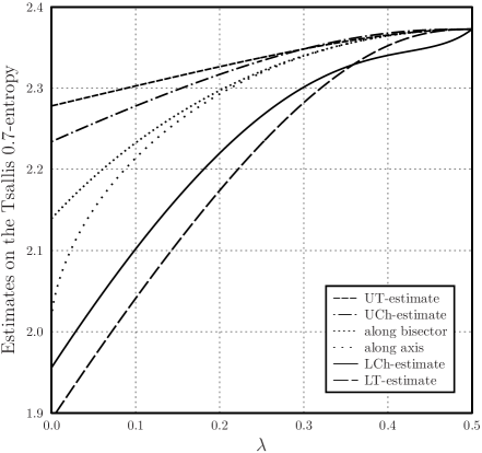
Figure 1: Estimates on the Tsallis $0.7$-entropy versus $\lambda$ for the $3$-design with $6$ vertices.

Further, we consider the $5$-design with $K=12$ vertices forming an icosahedron. In Fig. 2, we plot the two lower estimates and the two upper ones as functions of $\lambda$. The two-sided estimate (72) is better for states of moderate mixedness. Moreover, we see a range, where LCh-estimate is sufficiently poor in comparison with LT-estimate. For the Shannon entropies, LCh-estimate and LT-estimate do not differ so essentially rastpol . Nevertheless, one still has a wide domain, in which LCh-estimate is better. Relative differences of two-sided estimating do not exceed $5.2$ %. By two dotted lines, we also show values of the $0.7$-entropy for two orientations of the Bloch vector. Let the $z$-axis pass through two opposite vertices and form symmetry axis of icosahedron. Let the $x$-axis pass so that one of inclined edges lies in the $zx$-plane. One of the used orientations is along the $z$-axis, whereas the other is along positive part of the $x$-axis. For the maximally mixed state, all the curves converge at one point.

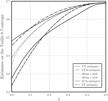
Figure 2: Estimates on the Tsallis $0.7$-entropy versus $\lambda$ for the $5$-design with $12$ vertices.

Further, we recall the $7$-design with $K=24$ vertices of deformed snub cube as described in section 3 of hardin96 . Its faces contains $6$ squares and $32$ triangles. In Fig. 3, we plot the estimates of interest versus $\lambda$. The two-sided estimate (72) is better only for states of low mixedness. There is again a range, where LCh-estimate is relatively poor. On the other hand, both the LCh- and UCh-estimates are still better for pure states. It is well known that bounds for pure states play an important role in deriving separability criteria and steering inequalities. In details, we will address this question later. Relative differences of two-sided estimating are no greater than $2.9$ %. By two dotted lines, we also show values of the $0.7$-entropy for two orientations of the Bloch vector. The first direction goes to the square core, whereas the other goes to center of of one of square edges. In this example, the two dotted lines are closer than in Fig. 2. All six curves tend to coincide on the right. Distinctions between them are less than in other examples.

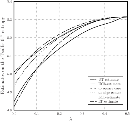
Figure 3: Estimates on the Tsallis $0.7$-entropy versus $\lambda$ for the $7$-design with $24$ vertices.

The above examples allow us to make several conclusions. We see that the LCh- and UCh-estimates provide better results for pure states and states close to them. For states of sufficient mixedness, the LT- and UT-estimates should be preferred. With growth of degree $t$, more restrictions are actually imposed on the probabilities. Their distribution becomes more uniform, though number of outcomes also grows. This fact leads to shifting points of approximation closer to the right point $x=1$. So, we observe increasing role of the estimates with coefficients according to the Taylor scheme. Nevertheless, the estimates with flexible coefficients still remain better for pure states. It is well known that pure-state entropic bounds are significant to derive separability and steering criteria. Hence, the LCh- and UCh-estimates are of interest, even if domains of their dominance shorten. In the next section, we will consider separability criteria and steering inequalities in more detail.

Figure 4: Estimates on the Tsallis $1.3$-entropy versus $\lambda$ for the $3$-design with $6$ vertices.

Finally, we briefly exemplify the derived estimates for a value of the range $\alpha\in(1,2)$. In Fig. 4, the four estimates from (71) and (72) are plotted for $\alpha=1.3$ together with the actual entropies for two orientations of the Bloch vector. Here, relative differences of two-sided estimating are no more than $3.9$ %. Overall, both the approaches to estimate $\alpha$-entropies demonstrate domains of utility, though the estimate (72) is better only for states very close to the maximally mixed one. Entropies themselves and estimates on them do not differ so essentially as in Fig. 1. In that figure, the graph of LCh-estimate shows a fairly convex part at the right end of the interval. In Fig. 4, this behavior is not expressed so brightly. By some inspection, similar observations can be made for other examples of quantum designs in two dimensions. We refrain from presenting the details here.

By comparison, the two approaches to estimate $\alpha$-entropies are more different for $\alpha\in(0,1)$. Indeed, the first derivative of $\eta_{\alpha}(x)$ is not finite for $x\to+0$ and $\alpha\in(0,1)$. On the other hand, derivatives of any polynomial are certainly finite, whence the slope of tangential line is enough far from the vertical. For $\alpha\in(0,1)$, therefore, our approximation have to be relatively poor in some right neighborhood of the left point $x=0$. By its origin, the Taylor scheme provides the best way around the right point $x=1$. The polynomials with flexible coefficients give better results closely to the left point of the interval. Similar observations were made for the Shannon entropy rastpol . For $\alpha\in(1,2)$, the first derivative of $\eta_{\alpha}(x)$ remains finite for $x\to+0$, so that both the schemes allow to estimate $\alpha$-entropy in a good way. As some inspection shows, we should prefer (71) for sufficiently small values of $\alpha$. For non-integer values $\alpha>2$, one can use the methods already presented in the literature.

V Some applications of the main results

In this section, we consider applications of the derived relations for tasks of quantum information. It was discussed in rastpol how to use design-structured POVMs for estimating the von Neumann entropy of a quantum state. Due to (71) and (72), the same measurements can be used for estimating generalized quantum entropies. To the given density matrix $\boldsymbol{\rho}$ and $0<\alpha\neq 1$, we assign the Tsallis $\alpha$-entropy

$${\mathrm{H}}_{\alpha}(\boldsymbol{\rho}):=\frac{\mathrm{tr}(\boldsymbol{\rho}^{\alpha})-1}{1-\alpha}\ .$$ (75)

The quantum Rényi $\alpha$-entropy reads as

$${\mathrm{R}}_{\alpha}(\boldsymbol{\rho}):=\frac{\ln\bigl{(}\mathrm{tr}(\boldsymbol{\rho}^{\alpha})\bigr{)}}{1-\alpha}=\frac{1}{1-\alpha}\,\ln\bigl{(}1+(1-\alpha){\mathrm{H}}_{\alpha}(\boldsymbol{\rho})\bigr{)}\,.$$ (76)

In the limit $\alpha\to 1$, both the above formulas gives the von Neumann entropy ${\mathrm{H}}_{1}(\boldsymbol{\rho})=\!{}-\mathrm{tr}(\boldsymbol{\rho}\ln\boldsymbol{\rho})$. Using quantities of the form (11) or (12), one can recalculate the traces $\mathrm{tr}(\boldsymbol{\rho}^{s})$ for $s=2,\ldots,t$. Applying (71) and (72) to this case results in

$$\sum_{s=1}^{t}a_{t\alpha}^{(s)}\Lambda^{\alpha-s}\,\mathrm{tr}(\boldsymbol{\rho}^{s})-\Lambda^{\alpha-1}\ln_{\alpha}(\Lambda) \leq{\mathrm{H}}_{\alpha}(\boldsymbol{\rho})\leq{b}_{t\alpha}^{(0)}\Lambda^{\alpha}d+\sum_{s=1}^{t}b_{t\alpha}^{(s)}\Lambda^{\alpha-s}\,\mathrm{tr}(\boldsymbol{\rho}^{s})-\Lambda^{\alpha-1}\ln_{\alpha}(\Lambda)\,,$$ (77)

$$\sum_{s=1}^{t}{\tilde{a}}_{t\alpha}^{(s)}\Lambda^{\alpha-s}\,\mathrm{tr}(\boldsymbol{\rho}^{s})-\Lambda^{\alpha-1}\ln_{\alpha}(\Lambda) \leq{\mathrm{H}}_{\alpha}(\boldsymbol{\rho})\leq{\tilde{b}}_{t\alpha}^{(0)}\Lambda^{\alpha}d+\sum_{s=1}^{t}{\tilde{b}}_{t\alpha}^{(s)}\Lambda^{\alpha-s}\,\mathrm{tr}(\boldsymbol{\rho}^{s})-\Lambda^{\alpha-1}\ln_{\alpha}(\Lambda)\,,$$ (78)

where $\alpha\in(0,2)$ and $\Lambda=\Upsilon_{d-1}^{(t)}\bigl{(}\mathrm{tr}(\boldsymbol{\rho}^{\!\;t})\bigr{)}$. The latter estimates the eigenvalues of $\boldsymbol{\rho}$ from above rastpol . Similarly to (65), we have

$$\frac{1}{1-\alpha}\,\ln\bigl{(}1+(1-\alpha){\mathrm{A}}_{n\alpha}(\boldsymbol{\rho})\bigr{)}\leq{\mathrm{H}}_{\alpha}(\boldsymbol{\rho})\leq\frac{1}{1-\alpha}\,\ln\bigl{(}1+(1-\alpha){\mathrm{B}}_{n\alpha}(\boldsymbol{\rho})\bigr{)}\,,$$ (79)

whenever ${\mathrm{A}}_{n\alpha}(\boldsymbol{\rho})\leq{\mathrm{H}}_{\alpha}(\boldsymbol{\rho})\leq{\mathrm{B}}_{n\alpha}(\boldsymbol{\rho})$. Here, the term ${\mathrm{A}}_{n\alpha}(\boldsymbol{\rho})$ stands for the left-hand side of (77) or (78), and the term ${\mathrm{B}}_{n\alpha}(\boldsymbol{\rho})$ stands for the right-hand side of (77) or (78). In this way, the quantum Rényi $\alpha$-entropy of order $\alpha\in(0,2)$ can be estimated.

The phenomenon of entanglement attracts an attention since the Schrödinger “cat paradox” paper erwin1935 and in the Einstein–Podolsky-Rosen paper epr1935 were published. Also, it is an indispensable tool for quantum information processing hhhh09 . Many separability conditions follow from uncertainty relations glew04 ; giov04 ; devs05 ; gmta06 . A bipartite mixed state is called separable, when its density matrix can be represented as a convex combination of product states werner89 ; zhsl98 . To derive separability conditions from (71) and (72), we recall the scheme proposed in rastsep . Let ${\mathcal{N}}_{A}=\{{\mathsf{N}}_{Aj}\}$ and ${\mathcal{N}}_{B}=\{{\mathsf{N}}_{Bk}\}$ be two $K$-outcome POVMs in ${\mathcal{H}}_{A}$ and ${\mathcal{H}}_{B}$, respectively. It is helpful to numerate POVM elements by numbers from $0$ up to $K-1$. To the given POVMs, we assign the measurement ${\mathcal{M}}({\mathcal{N}}_{A},{\mathcal{N}}_{B})$ with $K$ elements

$${\mathsf{M}}_{k}:=\sum_{j=0}^{K-1}{\mathsf{N}}_{Aj}\otimes{\mathsf{N}}_{Bk\ominus{j}}\,,$$ (80)

where the symbol $\ominus$ means the modular subtraction. It follows from (80) that rastsep

$${\mathtt{p}}\bigl{(}{\mathcal{M}};\boldsymbol{\rho}_{A}\otimes\boldsymbol{\rho}_{B}\bigr{)}={\mathtt{p}}({\mathcal{N}}_{A};\boldsymbol{\rho}_{A})*{\mathtt{p}}({\mathcal{N}}_{B};\boldsymbol{\rho}_{B})\,.$$ (81)

That is, for product states one generates the convolution of two distributions assigned to local measurements. Hence, the distribution (81) is majorized by any of two local probability distributions rastsep . Let one of two POVMs ${\mathcal{N}}_{A}$ and ${\mathcal{N}}_{B}$, say ${\mathcal{N}}_{A}$, be assigned to a quantum design in line with (5). To get separability conditions, we need state-independent uncertainty bounds. As was already noted, validity of the lower entropic bounds (73) and (74) for all states should be checked in each concrete example. If they really give a state-independent formulation, then we have the following result. For each separable state $\boldsymbol{\rho}_{AB}$ and $\alpha\in(0,2)$, it holds that

$$H_{\alpha}({\mathcal{M}};\boldsymbol{\rho}_{AB}) \geq\sum_{s=1}^{t}a_{t\alpha}^{(s)}\Upsilon^{\alpha-s}K^{1-s}d^{\,s}\,{\mathcal{D}}_{d}^{(s)}-\Upsilon^{\alpha-1}\ln_{\alpha}(\Upsilon)\,,$$ (82)

$$H_{\alpha}({\mathcal{M}};\boldsymbol{\rho}_{AB}) \geq\sum_{s=1}^{t}{\tilde{a}}_{t\alpha}^{(s)}\Upsilon^{\alpha-s}K^{1-s}d^{\,s}\,{\mathcal{D}}_{d}^{(s)}-\Upsilon^{\alpha-1}\ln_{\alpha}(\Upsilon)\,,$$ (83)

where $d=\dim({\mathcal{H}}_{A})$ and $\Upsilon=\Upsilon_{K-1}^{(t)}\bigl{(}K^{1-t}d^{\,t}\,{\mathcal{D}}_{d}^{(t)}\bigr{)}$. The separability criteria (82) and (83) respectively follow from (73) and (74) by Schur-concavity and concavity of the Tsallis $\alpha$-entropy. The proof is carried out quite similarly to proposition 8 of the paper rastsep . Another way is based on uncertainty relations of the Landau–Pollak type devs05 . It follows from the results of rastdes that

$$\underset{k}{\max}\,p_{k}({\mathcal{N}}_{A};\boldsymbol{\rho}_{A})\leq\Upsilon_{K-1}^{(t)}\bigl{(}\bar{\beta}^{(t)}(\boldsymbol{\rho}_{A})\bigr{)}\leq\Upsilon_{K-1}^{(t)}\bigl{(}K^{1-t}d^{\,t}\,{\mathcal{D}}_{d}^{(t)}\bigr{)}\,.$$ (84)

That is, we a priori know estimating from above that holds for all states. For any separable state $\boldsymbol{\rho}_{AB}$, therefore, we have

$$\underset{k}{\max}\,p_{k}({\mathcal{M}};\boldsymbol{\rho}_{AB})\leq\Upsilon_{K-1}^{(t)}\bigl{(}K^{1-t}d^{\,t}\,{\mathcal{D}}_{d}^{(t)}\bigr{)}\,.$$ (85)

The above separability criteria mirror conditions imposed on measurement statistics in the case of a single POVM. Quantum designs also give a tool to characterize multipartite entanglement kwg20 . Applications of the derived complementarity relations to multipartite systems deserve further investigations.

The question of using quantum designs to derive quantum steering inequalities was addressed in guhne20 ; rastdes ; rastpol . Quantum steering inequalities are currently the subject of active research. For more details, see the reviews cs2017 ; ucno20 and references therein. It is natural that steering criteria are closely linked to uncertainty relations. Steering inequalities in terms of Shannon entropies were considered in sbwch13 ; kdr15 ; rmm18 . Steering criteria also follow from uncertainty relations using generalized entropies, including both the Tsallis cug18 and Rényi entropies brun18 . The novel uncertainty relations presented in this paper can immediately be incorporated into the frameworks developed in cug18 ; brun18 . Here, we refrain from delving into details of this multifaceted issue.

Finally, we consider the case of detection inefficiencies, when the “no-click” event sometimes happens rastmubs . To the given detector efficiency $\varkappa\in[0.5,1]$ and distribution ${\mathtt{p}}=\{p_{j}\}$, we assign a “distorted” distribution ${\mathtt{p}}^{(\varkappa)}$ such that

$$p_{j}^{(\varkappa)}=\varkappa\,p_{j}\,,\qquad p_{\varnothing}^{(\varkappa)}=1-\varkappa\,.$$ (86)

The probability $p_{\varnothing}^{(\varkappa)}$ characterizes the no-click event. Indices of the form (58) are then altered as

$$I^{(s)}\bigl{(}{\mathtt{p}}^{(\varkappa)}\bigr{)}=\varkappa^{s}I^{(s)}({\mathtt{p}})+(1-\varkappa)^{s}\,.$$ (87)

Altered indices are really dealt with in applications of the presented complementarity relations. So, a special attention should be paid to determining actual $\varkappa$ as accurately as possible. Substituting this value, the original indices $I^{(s)}({\mathtt{p}})$ are extracted due to (87). After that, we are ready to apply the complementarity relations in practical questions of quantum information processing. Of course, used detectors must have sufficiently high efficiency.

VI Conclusions

We have obtained complementarity relations for POVMs assigned to a quantum design. To express the amount of uncertainties quantitatively, the Rényi and Tsallis entropies of order $\alpha\in(0,2)$ were used. The two methods to estimate functions of interest were utilized. The first method is based on truncated expansions of the Taylor type. The second way uses polynomials with flexible coefficients. Within applied analysis, such expansions were motivated and illustrated by Lanzos lanczos . Both the methods lead to two-sided estimates on the Tsallis and Rényi entropies, whenever several indices of subsequent integer degrees are prescribed. Design-structured POVMs are an obvious example in which this situation occurs. Hence, the complementarity relations for related measurements in terms of generalized entropies of order $\alpha\in(0,2)$ are naturally. They give a natural extension of the main results of rastpol . The derived two-sided estimates are useful in any context, where the sums of certain powers of probabilities are easy to obtain.

The presented complementarity relations were exemplified with several quantum designs in two dimensions. It was observed that the two methods of estimating are more different for $\alpha\in(0,1)$. With growth of degree $t$, we see a reduction of the domain, where the second way is better. On the other hand, the scheme of polynomials with flexible coefficients remains important to estimate $\alpha$-entropies for a pure state. As is well known, pure-state entropic bounds are used to derive separability criteria and steering inequalities. Hence, the second scheme to formulate two-sided estimates will be interesting, even if a domain of its role shortens. Possible applications of new relations in quantum tomography and entanglement detection were illustrated. As was also mentioned, novel entropic steering inequalities follow from the derived relations. All these results newly show a utility of polynomials with flexible coefficients initially proposed by Lanzos lanczos .

Appendix A An inequality

Let us consider the polynomial function of $x\in[0,1]$ defined as

$$\phi_{n}(x)=\sum_{s=2}^{n}\frac{c_{n}^{(s)}x^{s}}{s-1}\ ,$$ (88)

where $n\geq 2$. It is immediate to obtain

$$\frac{{\mathrm{d}}^{2}\phi_{n}(x)}{{\mathrm{d}}{x}^{2}}=\sum_{s=2}^{n}s\,c_{n}^{(s)}x^{s-2}=\frac{1}{x}\left(\frac{{\mathrm{d}}{T}_{n}^{*}(x)}{{\mathrm{d}}{x}}-c_{n}^{(1)}\right).$$ (89)

In terms of $\xi=2x-1=\cos\theta$ with $\theta\in[0,\pi]$, we have $T_{n}^{*}(x)=T_{n}(\cos\theta)=\cos{n}\theta$ and

$$\frac{{\mathrm{d}}{T}_{n}^{*}(x)}{{\mathrm{d}}{x}}=\frac{2\,{\mathrm{d}}{T}_{n}(\xi)}{{\mathrm{d}}\xi}=\frac{2\,{\mathrm{d}}\theta}{{\mathrm{d}}\cos\theta}\,\frac{{\mathrm{d}}\cos{n}\theta}{{\mathrm{d}}\theta}=\frac{2n\sin{n}\theta}{\sin\theta}\ .$$ (90)

Combining this with $c_{n}^{(1)}=(-1)^{n+1}2n^{2}$ and (89) leads to

$$\frac{x\sin\theta}{2n}\>\frac{{\mathrm{d}}^{2}\phi_{n}(x)}{{\mathrm{d}}{x}^{2}}=(-1)^{n}\Bigl{[}n\sin\theta+(-1)^{n}\sin{n}\theta\Bigr{]}\,.$$ (91)

It can be shown by induction that, for $\theta\in[0,\pi]$ and integer $n\geq 1$,

$$\left|\sin{n}\theta\right|\leq{n}\sin\theta\,.$$ (92)

In view of (92), the sign of (91) is determined by $(-1)^{n}$. For $x\in[0,1]$, therefore, the function $\phi_{n}(x)$ is convex for even $n$ and concave for odd $n$. Hence, we also see convexity of the right-hand side of (30). Due to $\phi_{n}(0)=0$ and $\left.{\mathrm{d}}\phi_{n}/{\mathrm{d}}{x}\,\right|_{x=0}=0$, the tangent line is horizontal at the point $x=0$ and coincides with the abscissa. Combining this with convexity and concavity, respectively, one gets $\phi_{n}(x)\geq 0$ for even $n$ and $\phi_{n}(x)\leq 0$ for odd $n$. In other words, for all $x\in[0,1]$ we have

$$(-1)^{n}\phi_{n}(x)\geq 0\,.$$ (93)

For integer $r\geq 1$, we further define

$$\varphi_{n}^{(r)}(x)=(-1)^{n}\sum_{s=2}^{n}\frac{c_{n}^{(s)}x^{s}}{(s-1)^{r}}\ ,$$ (94)

so that the left-hand side of (93) coincides with $\varphi_{n}^{(1)}(x)$. For $x\in[0,1]$, one has

$$\varphi_{n}^{(r)}(x)\geq 0\,,$$ (95)

This conclusion is obtained by induction due to (93) and

$$\varphi_{n}^{(r+1)}(x)=\int_{0}^{x}\varphi_{n}^{(r)}(z)\,\frac{{\mathrm{d}}{z}}{z^{2}}\ .$$

Assuming $\alpha-1=\gamma\in[0,1)$, we now write the power expansion

$$\frac{(-1)^{n}}{\tau_{n\alpha}}=2n^{2}+(-1)^{n}\gamma\,\sum_{s=2}^{n}\frac{c_{n}^{(s)}}{s-1-\gamma}=2n^{2}+(-1)^{n}\gamma\,\sum_{s=2}^{n}\frac{c_{n}^{(s)}}{s-1}\left(1-\frac{\gamma}{s-1}\right)^{\!-1}=2n^{2}+\sum_{r=1}^{\infty}\varphi_{n}^{(r)}(1)\,\gamma^{r}\,.$$ (96)

Due to (95), the right-hand side of (96) is positive. That is, we proved $(-1)^{n}\,\tau_{n\alpha}\geq 0$ for $\alpha\in[1,2)$.

References

- (1) Heisenberg W. Über den anschaulichen Inhalt der quantentheoretischen Kinematik und Mechanik. Z. Phys. 43, 172–198 (1927)
- (2) Kennard, E.H.: Zur Quantenmechanik einfacher Bewegungstypen. Z. Phys. 44, 326–352 (1927)
- (3) Robertson, H.P.: The uncertainty principle. Phys. Rev. 34, 163–164 (1929)
- (4) D. Deutsch, Uncertainty in quantum measurements. Phys. Rev. Lett. 50, 631 (1983)
- (5) H. Maassen, J.B.M. Uffink, Generalized entropic uncertainty relations. Phys. Rev. Lett. 60, 1103 (1988)
- (6) S. Wehner, A. Winter, Entropic uncertainty relations – a survey. New J. Phys. 12, 025009 (2010)
- (7) P.J. Coles, M. Berta, M. Tomamichel, S. Wehner, Entropic uncertainty relations and their applications. Rev. Mod. Phys. 89, 015002 (2017)
- (8) I. Białynicki-Birula, Ł. Rudnicki, Entropic uncertainty relations in quantum physics. In: Statistical Complexity, ed. K.D. Sen, 1–34 (Springer, Berlin, 2011)
- (9) A. Hertz, N.J. Cerf, Continuous-variable entropic uncertainty relations. J. Phys. A: Math. Theor. 52, 173001 (2019)
- (10) T. Durt, B.-G. Englert, I. Bengtsson, K. Życzkowski, On mutually unbiased bases. Int. J. Quantum Inf. 8, 535 (2010)
- (11) J. Renes, R. Blume-Kohout, A. Scott, C. Caves, Symmetric informationally complete quantum measurements. J. Math. Phys. 45, 2171 (2004)
- (12) C.A. Fuchs, M.C. Hoang, B.C. Stacey, The SIC question: history and state of play. Axioms 6, 21 (2017)
- (13) P. Horodecki, Ł. Rudnicki, K. Życzkowski, Five open problems in quantum information. E-print arXiv:2002.03233 [quant-ph] (2020)
- (14) A. Ambainis, J. Emerson, Quantum -designs: -wise independence in the quantum world. E-print arXiv:quant-ph/0701126 (2007)
- (15) D. Gross, K. Audenaert, J. Eisert, Evenly distributed unitaries: on the structure of unitary designs. J. Math. Phys. 48, 052104 (2007)
- (16) A.J. Scott, Optimizing quantum process tomography with unitary 2-designs. J. Phys. A: Math. Theor. 41, 055308 (2008)
- (17) C. Dankert, R. Cleve, J. Emerson, E. Livine, Exact and approximate unitary 2-designs and their application to fidelity estimation. Phys. Rev. A 80, 012304 (2009)
- (18) A. Roy, A.J. Scott, Unitary designs and codes, Des. Codes Cryptogr. 53, 13–31 (2009)
- (19) B. Vermersch, A. Elben, M. Dalmonte, J.I. Cirac, P. Zoller, Unitary -designs via random quenches in atomic Hubbard and spin models: Application to the measurement of Rényi entropies. Phys. Rev. A 97, 023604 (2018)
- (20) J. Bae, B.C. Hiesmayr, D. McNulty, Linking entanglement detection and state tomography via quantum 2-designs. New J. Phys. 21, 013012 (2019)
- (21) A. Ketterer, N. Wyderka, O. Gúhne, Characterizing multipartite entanglement with moments of random correlations. Phys. Rev. Lett. 122, 120505 (2019)
- (22) J. Czartowski, D. Goyeneche, M. Grassl, K. Życzkowski, Isoentangled mutually unbiased bases, symmetric quantum measurements, and mixed-state designs. Phys. Rev. Lett. 124, 090503 (2019)
- (23) A.J. Scott, Tight informationally complete quantum measurements. J. Phys. A: Math. Gen. 39, 13507 (2006)
- (24) A. Ketterer, O. Gühne, Entropic uncertainty relations from quantum designs. Phys. Rev. Research 2, 023130 (2020)
- (25) A.E. Rastegin, Rényi formulation of uncertainty relations for POVMs assigned to a quantum design. J. Phys. A: Math. Theor. 53, 405301 (2020)
- (26) A.E. Rastegin, On estimating the Shannon entropy and (un)certainty relations for design-structured POVMs. E-print arXiv:2009.13187 [quant-ph] (2020)
- (27) A.E. Rastegin, Uncertainty and certainty relations for quantum coherence with respect to design-structured POVMs. J. Phys.: Conf. Ser. 1847, 012044 (2021)
- (28) C. Lanczos, Applied Analysis (Dover, New York, 2010)
- (29) P.D. Seymour, T. Zaslavsky, Averaging sets: A generalization of mean values and spherical designs. Adv. Math. 52, 213 (1984)
- (30) R.H. Hardin, N.J.A. Sloane, McLaren’s improved snub cube and other new spherical designs in three dimensions. Discrete Comput. Geom. 15, 429 (1996)
- (31) A.E. Rastegin, Uncertainty relations for MUBs and SIC-POVMs in terms of generalized entropies. Eur. Phys. J. D 67, 269 (2013)
- (32) R.L. Graham, D.E. Knuth, O. Patashnik, Concrete Mathematics (Addison-Wesley, New York, 1994)
- (33) C. Tsallis, Possible generalization of Boltzmann–Gibbs statistics. J. Stat. Phys. 52, 479–487 (1988)
- (34) A. Rényi, On measures of entropy and information. In: Proc. of the 4th Berkeley Symposium on Mathematical Statistics and Probability, ed. J. Neyman, Vol. I., 547–561 (University of California Press, Berkeley, 1961)
- (35) I. Bengtsson, K. Życzkowski, Geometry of Quantum States: An Introduction to Quantum Entanglement (Cambridge University Press, Cambridge, 2017)
- (36) P. Harremoës, F. Topsøe, Inequalities between entropy and index of coincidence derived from information diagrams. IEEE Trans. Inf. Theory 47, 2944 (2001)
- (37) E. Schrödinger, Die gegenwärtige situation in der quantenmechanik. Naturwissenschaften 23, 807–812, 823–828, 844–849 (1935)
- (38) A. Einstein, B. Podolsky, N. Rosen, Can quantum-mechanical description of physical reality be considered complete? Phys. Rev. 47, 777–780 (1935)
- (39) R. Horodecki, P. Horodecki, M. Horodecki, K. Horodecki, Quantum entanglement. Rev. Mod. Phys. 81, 865–942 (2009)
- (40) O. Gühne, M. Lewenstein, Entropic uncertainty relations and entanglement. Phys. Rev. A 70, 022316 (2004)
- (41) V. Giovannetti, Separability conditions from entropic uncertainty relations. Phys. Rev. A 70, 012102 (2004)
- (42) J.I. de Vicente, J. Sánchez-Ruiz, Separability conditions from the Landau–Pollak uncertainty relation. Phys. Rev. A 71, 052325 (2005)
- (43) O. Gühne, M. Mechler, G. Tóth, P. Adam, Entanglement criteria based on local uncertainty relations are strictly stronger than the computable cross norm criterion. Phys. Rev. A 74, 010301(R) (2006)
- (44) R.F. Werner, Quantum states with Einstein–Podolsky–Rosen correlations admitting a hidden-variable model. Phys. Rev. A 40, 4277–4281 (1989)
- (45) K. Życzkowski, P. Horodecki, A. Sanpera, M. Lewenstein, Volume of the set of separable states. Phys. Rev. A 58, 883–892 (1998)
- (46) A.E. Rastegin, Rényi and Tsallis formulations of separability conditions in finite dimensions. Quantum Inf. Process. 16, 293 (2017)
- (47) A. Ketterer, N. Wyderka, O. Gühne, Entanglement characterization using quantum designs. Quantum 4, 325 (2020)
- (48) D. Cavalcanti, P. Skrzypczyk, Quantum steering: a review with focus on semidefinite programming, Rep. Prog. Phys. 80, 024001 (2017)
- (49) R. Uola, A.C.S. Costa, H.C. Nguyen, O. Gühne, Quantum steering. Rev. Mod. Phys. 92, 15001 (2020)
- (50) J. Schneeloch, C.J. Broadbent, S.P. Walborn, E.G. Cavalcanti, J.C. Howell, Einstein–Podolsky–Rosen steering inequalities from entropic uncertainty relations, Phys. Rev. A 87, 062103 (2013)
- (51) H.S. Karthik, A.R.U. Devi, A.K. Rajagopal, Joint measurability, steering, and entropic uncertainty, Phys. Rev. A 91, 012115 (2015)
- (52) A. Riccardi, C. Macchiavello, L. Maccone, Multipartite steering inequalities based on entropic uncertainty relations, Phys. Rev. A 97, 052307 (2018)
- (53) A.C.S. Costa, R. Uola, O. Gühne, Steering criteria from general entropic uncertainty relations. Phys. Rev. A 98, 050104(R) (2018)
- (54) T. Kriváchy, F. Fröwis, N. Brunner, Tight steering inequalities from generalized entropic uncertainty relations. Phys. Rev A 98, 062111 (2018)