KUNS-2887

Tensor network approach to 2D Yang-Mills theories

Masafumi Fukuma¹, Daisuke Kadoh^2,3 and Nobuyuki Matsumoto⁴

¹Department of Physics, Kyoto University, Kyoto 606-8502, Japan ²Faculty of Sciences and Engineering, Doshisha University, Kyoto 610-0394, Japan ³Research and Educational Center for Natural Sciences,
Keio University, Yokohama 223-8521, Japan ⁴RIKEN/BNL Research center, Brookhaven National Laboratory, Upton, NY 11973, USA

We propose a novel tensor network representation for two-dimensional Yang-Mills theories with arbitrary compact gauge groups. In this method, tensor indices are directly given by group elements with no direct use of the character expansion. We apply the tensor renormalization group method to this tensor network for $SU(2)$ and $SU(3)$, and find that the free energy density and the energy density are accurately evaluated. We also show that the singular value decomposition of a tensor has a group theoretic structure and can be associated with the character expansion.

1 Introduction

The tensor network (TN) method [1, 2, 3, 4, 5] is an attractive approach for studying many body systems, because it is free from the sign problem in the first place, and has a potential to precisely investigate critical phenomena in the large volume limit. In field theory, the tensor renormalization group (TRG) method [3] and its variations [6, 7, 8] are widely used to study various models such as the Schwinger model [9, 10, 11, 12], the Gross-Neveu and NJL models [13, 14], scalar field theories [15, 16, 17, 18], the Yang-Mills and gauge-Higgs models [19, 20], the Wess-Zumino model [21], and other related models [22, 23, 24].

For gauge groups $U(1)$ [9, 10, 11, 22, 25] and $SU(2)$ [19, 20], the character expansion was employed to represent the partition function with a tensor network. However, since the character expansion becomes a demanding task for higher-rank gauge groups, it remains as a difficult issue to apply the TN method to $SU(N)$ gauge theory for $N\geq 3$ including QCD.

In this paper, we propose a novel method to create a tensor network for two-dimensional Yang-Mills theory with no direct use of the character expansion. The Haar measure is discretized, and the group integration is replaced by a summation over $K$ randomly generated configurations. Then, the plaquette is regarded as a rank-$4$ tensor whose index runs from $1$ to $K$, and the set of plaquettes constitutes a tensor network. We test our method for $SU(2)$ and $SU(3)$ gauge groups, and find that the free energy density and the energy density agree very well with exact results. We also clarify the mathematical structure behind our method.

This paper is organized as follows. In Sec. 2, we introduce our tensor network representation for two-dimensional Yang-Mills theories with arbitrary compact gauge groups $G$, and discuss its relation with the character expansion. In Sec. 3, we test our method for $G=SU(2)$ and $G=SU(3)$. Section 4 is devoted to summary and discussion. Appendices provide some useful formulas in group theory.

2 Tensor network representations for 2D Yang-Mills theories

In this section, we introduce a new tensor network representation for two-dimensional Yang-Mills theories, and discuss its relation with the character expansion. We exclusively consider pure Yang-Mills theory for simplicity. It is straightforward to extend our method to systems with interacting matter fields.

2.1 Method

We consider the Yang-Mills theory with a compact gauge group $G$ on an infinite lattice $\Gamma\equiv\{n=(n_{1},n_{2})\,|\,n_{\mu}\in{\mathbb{Z}}~{}(\mu=1,2)\}$. The lattice spacing $a$ is set to $a=1$ unless otherwise noted, and $\hat{\mu}$ is the unit vector in the $\mu$ direction.

Let $U_{\mu}(n)$ be the $G$-valued link field on links $(n,n+\hat{\mu})$. The lattice action (the Wilson action) is given by

$$S=\frac{\beta}{N}\,\sum_{n\in\Gamma}{\rm Re\,tr}\,[1-U_{P}(n)],$$ (2.1)

where $U_{P}(n)$ is the plaquette field,

$$U_{P}(n)=U_{1}(n)\,U_{2}(n+\hat{1})\,U_{1}^{\dagger}(n+\hat{2})\,U_{2}^{\dagger}(n).$$ (2.2)

The partition function is defined as $Z=\int DU\,e^{-S}$, where $DU\equiv\prod_{n\in\Gamma}dU_{1}(n)\,dU_{2}(n)$ with $dU$ the Haar measure of $G$. Note that the partition function $Z$ can be written in the form of a tensor network with indices continuously taking values in $G$,

$$Z={\mathfrak{T}}{\mathfrak{r}}\prod_{n\in\Gamma}{\mathfrak{T}}_{g(n)h(n)g^{\prime}(n)h^{\prime}(n)},$$ (2.3)

where

$${\mathfrak{T}}_{g_{1}g_{2}g_{3}g_{4}}=e^{-(\beta/N)\,{\rm Re\,tr\,}(1-g_{1}g_{2}g_{3}^{{\dagger}}g_{4}^{{\dagger}})}$$ (2.4)

and ${\mathfrak{T}}{\mathfrak{r}}$ stands for the group integrations for $g(n),h(n)\in G$ $(n\in\Gamma)$ under a proper identification of indices.

We now discretize the Haar measure $dU$ to represent $Z$ as a tensor network with indices in a finite range:

$$\int dU\,f(U)\approx\frac{1}{K}\,\sum_{i=1}^{K}f(U_{i}),$$ (2.5)

where $\mathring{G}=\{U_{1},U_{2},\ldots,U_{K}\}$ consists of random points uniformly chosen from the group manifold. Applying Eq. (2.5) to the Haar measures in $DU$ leads to

$$Z\approx{\rm Tr}\prod_{n\in\Gamma}T_{i_{n}j_{n}i_{n}^{\prime}j_{n}^{\prime}},$$ (2.6)

where

$$T_{ijkl}=\frac{1}{K^{2}}e^{-(\beta/N)\,{\rm Re\,tr\,}(1-U_{i}U_{j}U_{k}^{\dagger}U_{l}^{\dagger})}$$ (2.7)

and $\rm Tr$ stands for the summation over $i_{n},j_{n}=1,2,\cdots,K$ for all $n\in\Gamma$ under the same identification of indices as above. As shown in Fig. 1, the tensor is assigned to each plaquette and has four indices corresponding to four links of the plaquette.

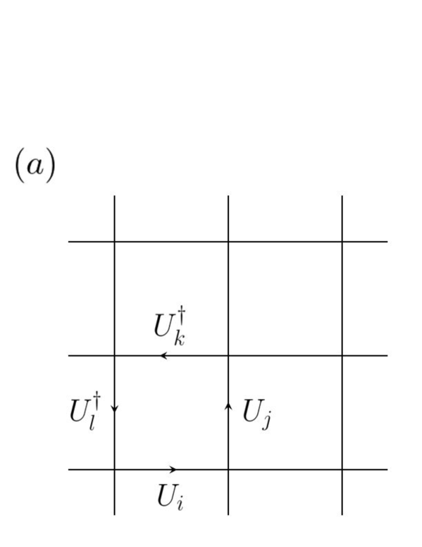
Figure 1: Two-dimensional square lattice. (a) A plaquette variable consisting of $U_{i},U_{j},U_{k},U_{l}$. (b) The corresponding tensor (2.7) assigned to the center of the plaquette.

Since our method is based on the discrete approximation with finite $K$, we check the convergence of the r.h.s. of Eq. (2.6) for large $K$ in actual numerical computations.

In the tensor network (2.6), a single set $\mathring{G}$ is commonly used to discretize all the $U_{\mu}(n)$-integrations. Actually, we can use a different set for each link. For example, tensors can be decomposed in different ways for even and odd sites [3], and we can use four different sets $\mathring{G}_{1},\mathring{G}_{2},\mathring{G}_{3},\mathring{G}_{4}$ to discretize the integrations at four links, $U_{i},\,U_{j},\,U_{k},\,U_{l}$, in Fig. 1. We then have

$$Z\approx{\rm Tr}\prod_{n\in\Gamma_{e}}T^{e}_{i_{n}j_{n}i^{\prime}_{n}j^{\prime}_{n}}\cdot\prod_{m\in\Gamma_{o}}T^{o}_{i_{m}j_{m}i^{\prime}_{m}j^{\prime}_{m}}$$ (2.8)

with

$$T^{e}_{ijkl}\equiv\frac{1}{K^{2}}\,e^{-(\beta/N){\rm Re\,Tr}(1-U^{(1)}_{i}U^{(2)}_{j}U^{(3){\dagger}}_{k}U^{(4){\dagger}}_{l})},$$ (2.9)

$$T^{o}_{ijkl}\equiv\frac{1}{K^{2}}\,e^{-(\beta/N){\rm Re\,Tr}(1-U^{(3)}_{i}U^{(4)}_{j}U^{(1){\dagger}}_{k}U^{(2){\dagger}}_{l})},$$ (2.10)

where $U^{(a)}_{i}\in\mathring{G}_{a}$ $(a=1,2,3,4)$ and $\Gamma_{e/o}$ are the set of even and odd sites, respectively. The introduction of four different sets significantly improve the precision of the results compared to a single set as presented in section 3.

Once the tensor network is obtained, any TRG method can be applied straightforwardly. In the Levin-Nave TRG, the singular value decomposition (SVD) is employed to decompose the tensors. In general, the SVD of an $n\times n$ matrix $M_{ij}$ is given by

$$M_{ij}=\sum_{a=1}^{n}\sigma_{a}U_{ia}V^{\ast}_{ja},$$ (2.11)

where $\sigma_{a}$ are singular values sorted as $\sigma_{1}\geq\sigma_{2}\geq\cdots\geq\sigma_{n}\geq 0$ and $U,\,V$ are unitary matrices. In our case, regarding $T^{e}_{ijkl}$ (resp. $T^{o}_{ijkl}$) as a matrix with the column $ij$ (resp. $jk$) and the row $kl$ (resp. $li$), we have

$$T^{e}_{ijkl} =\sum_{A=1}^{K^{2}}\sigma^{e}_{A}U^{e}_{ij,A}V^{e\,\ast}_{kl,A},$$ (2.12)

$$T^{o}_{ijkl} =\sum_{A=1}^{K^{2}}\sigma^{o}_{A}U^{o}_{jk,A}V^{o\,\ast}_{li,A}.$$ (2.13)

Figure 2 shows these decompositions. We again arrive at the tensor network of two-dimensional square lattice by defining the renormalized tensor $T^{(1)}$ with bond dimension $D$ as

$$T^{(1)}_{A_{1}A_{2}A_{3}A_{4}}=\sqrt{\sigma^{e}_{A_{1}}\sigma^{o}_{A_{2}}\sigma^{e}_{A_{2}}\sigma^{o}_{A_{4}}}\sum_{i,j,k,l=1}^{D}U^{e}_{ij,A_{1}}V^{o\,\ast}_{jk,A_{2}}V^{e\,\ast}_{kl,A_{3}}U^{o}_{li,A_{4}}.$$ (2.14)

The tensor network is repeatedly renormalized in this way.

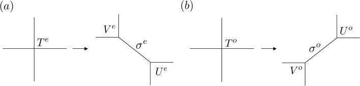
Figure 2: The SVDs of even tensor (a) and odd tensor (b).

Since the bond dimension of the initial tensors [Eqs. (2.9) and (2.10)] is $K$, the cost of the first SVD scales with $O(K^{6})$. Once the tensors are renormalized, the bond dimension changes to $D$. The cost of the subsequent iterations then scales with $O(D^{6})$.

2.2 Relation with the character expansion

To understand the group theoretic structure of the SVD in the previous subsection, we consider the limit $K\to\infty$, i.e., the case where the tensor indices continuously take all the values in $G$. See appendix A for a mathematical material necessary for the argument below.

Let $R$ be an irreducible unitary representation of $G$ with dimension $d_{R}$, and $D_{R}(U)=(D^{R}_{rs}(U))$ $(r,s=1,2,\ldots,d_{R}$) the representation matrix of $U$. Denoting the character of $R$ by $\chi_{R}(U)$, the function $e^{-(\beta/N)\,{\rm Re\,tr\,}(1-U)}$ can be expanded as

$$e^{-(\beta/N)\,{\rm Re\,tr\,}(1-U)}=\sum_{R}d_{R}\,\lambda_{R}(\beta)\chi_{R}(U).$$ (2.15)

Here and hereafter, $\sum_{R}$ stands for the summation over the irreducible representations $R$. The coefficients $\lambda_{R}(\beta)$ are given by

$$\lambda_{R}(\beta)=\frac{1}{d_{R}}\,\int dU\,e^{-(\beta/N)\,{\rm Re\,tr\,}(1-U)}\,\chi_{R}(U^{-1}),$$ (2.16)

as can be shown by using Eq. (A.8).

We again consider the infinite dimensional rank-$4$ tensor ${\mathfrak{T}}_{g_{1}g_{2}g_{3}g_{4}}$ [see Eq. (2.4)]. By using Eq. (2.15), this can be written as $\sum_{R}d_{R}\,\lambda_{R}\,\chi_{R}(g_{1}g_{2}g_{3}^{-1}g_{4}^{-1})$ and decomposed in two ways:

$${\mathfrak{T}}_{g_{1}g_{2}g_{3}g_{4}} =\sum_{A=(R,r,s)}{\mathfrak{U}}^{e}_{(g_{1},g_{2}),A}\,\lambda_{R}\,{\mathfrak{V}}^{e\,\ast}_{(g_{3},g_{4}),A}=\sum_{A=(R,r,s)}{\mathfrak{U}}^{o}_{(g_{2},g_{3}),A}\,\lambda_{R}\,{\mathfrak{V}}^{o\,\ast}_{(g_{4},g_{1}),A}$$ (2.17)

with

$${\mathfrak{U}}^{e}_{(g_{1},g_{2}),A}={\mathfrak{V}}^{e}_{(g_{2},g_{1}),A}={\mathfrak{U}}^{o}_{(g_{1},g_{2}^{-1}),A}={\mathfrak{V}}^{o}_{(g_{2},g_{1}^{-1}),A}\equiv\sqrt{d_{R}}\,D^{R}_{rs}(g_{1}g_{2}).$$ (2.18)

The Peter-Weyl theorem (see appendix A) states that the matrix $W_{g,A}\equiv\sqrt{d_{R}}\,D^{R}_{rs}(g)$ is unitary. Thus, together with the inequality $\lambda_{R}\geq 0$, we find that the decompositions (2.17) are actually SVDs. Then, the new tensor ${\mathfrak{T}}^{(1)}$ [Eq. (2.14) with $D=\infty$] is calculated by following Eqs. (2.12)–(2.14), and is found to be

$${\mathfrak{T}}^{(1)}_{A_{1}A_{2}A_{3}A_{4}}=\frac{\lambda_{R_{1}}^{2}}{d_{R_{1}}}\,\delta_{R_{1}R_{2}R_{3}R_{4}}\,\delta_{s_{1}s_{2}}\,\delta_{r_{2}s_{3}}\,\delta_{r_{3}r_{4}}\,\delta_{s_{4}r_{1}}.$$ (2.19)

Once this expression is obtained, one can perform the TRG iterations (see Appendix C) to obtain

$$Z=\sum_{R}\,\lambda_{R}(\beta)^{V}.$$ (2.20)

Recall that the TN representation [Eqs. (2.8)–(2.10)] is a discretization of Eqs. (2.3) and (2.4). Note that the singular values of the tensor ${\mathfrak{T}}_{g_{1}g_{2}g_{3}g_{4}}$ have a degeneracy of $d_{R}^{2}$ for each $R$ because both $r$ and $s$ in $W_{g,A}=\sqrt{d_{R}}\,D^{R}_{rs}(g)$ take $d_{R}$ values. This means that the singular values $\sigma_{A}$ of our tensor $T_{ijkl}$ [Eqs. (2.12) and (2.13)] must have this degeneracy approximately. We actually find this approximate degeneracy in numerical calculations presented in the next section.

3 Numerical results

In this section, we apply our method to the Yang-Mills theory with gauge group $G=SU(N)$ $(N=2,3)$ on a periodic square lattice. We construct the tensor network with four different sets $\mathring{G}_{a}\,(a=1,2,3,4)$ of $K$ random link variables [see the discussion after Eqs. (2.8)–(2.10)]. We evaluate the free energy density $f(\beta)\equiv(1/V)\ln Z(\beta)$ with the Levin-Nave TRG, and the energy density $e(\beta)\equiv-(\partial/\partial\beta)f(\beta)$ by taking numerical derivatives. Note that estimates have statistical errors in addition to the systematic errors coming from the finiteness of $K$ and bond dimension $D$. The statistical errors to be given below are obtained from five independent trials.

3.1 $SU(2)$

We first make a detailed analysis for $SU(2)$.

Figure 3 shows $f(\beta)$ for various volumes $V=L^{2}$ ($L=4,\,8,\,16,\,32,\,64$) with $\beta/V$ fixed to 0.01. The exact values are indicated by the gray dashed line. Figure 4 shows the relative errors to the exact values for the same calculation.

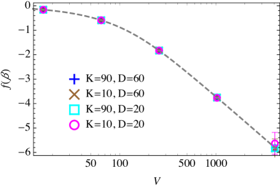
Figure 3: Volume dependence of $f(\beta)$ with $\beta/V=0.01$ for $SU(2)$. The exact values are expressed by the gray dashed line.

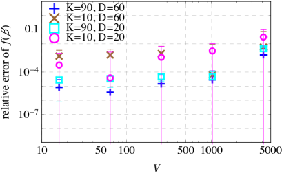
Figure 4: Relative error of the free energy density, $|f(\beta)-f_{\rm exact}(\beta)|\,/\,|f_{\rm exact}(\beta)|$, against volume $V$ with $\beta/V=0.01$ for $SU(2)$.

We see that the numerical results agree well with the exact values. We also see that as $V$ (and thus $\beta$) is increased, larger $K$ and $D$ are required to decrease the systematic errors. Figures 5 and 6 show the $K$, $D$ dependences of the free energy density at $V=64^{2}$ ($\beta=40.96$). We confirm that the numerical estimates approach the exact value in the limit $K\rightarrow\infty$ and $D\rightarrow\infty$.

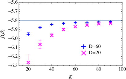
Figure 5: $K$ dependence of $f(\beta)$ with $\beta/V=0.01$ and $V=64^{2}$ ($\beta=40.96$) for $SU(2)$.

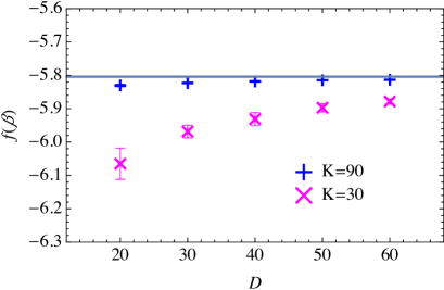
Figure 6: $D$ dependence of $f(\beta)$ with $\beta/V=0.01$ and $V=64^{2}$ ($\beta=40.96$) for $SU(2)$.

Having obtained the estimates for several values of $K$, we can make use of extrapolation to obtain a better estimate. Figure 7 shows the $\chi^{2}$ fit to the obtained data for $D=60$ with the scaling ansatz $g(K)\equiv\mu+\alpha K^{-p}$. Here, the fitting parameters $\alpha$, $\mu$ and $p$ are determined by minimizing the cost function

$$\chi^{2}(\mu,\alpha,p)\equiv\sum_{K=20,30,\cdots,90}\frac{[f(\beta;K)-g(K)]^{2}}{[\delta f(\beta;K)]^{2}},$$ (3.1)

where $f(\beta;K)$ is the obtained value for each $K$, and $\delta f(\beta;K)$ the statistical error.

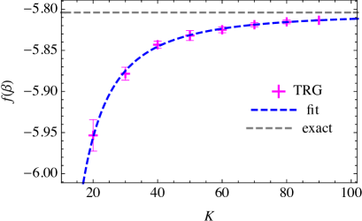
Figure 7: $\chi^{2}$ fit of the free energy densities $f(\beta)$ for various $K$ with $\beta/V=0.01$, $V=64^{2}$ and $D=60$ for $SU(2)$.

The value of $\mu$ is then used as the final estimate of $f(\beta)$.

The results of the fitting are summarized in Table 1.

	(exact)	$\mu$	$\alpha$	$p$	$\chi^{2}/{\rm DOF}$
$f(\beta)$	-5.8040	$-5.8045^{+0.0040}_{-0.0029}$	$-43^{+26}_{-60}$	$1.88^{+0.27}_{-0.28}$	0.13
$e(\beta)$	0.03639	$0.03655^{+0.00029}_{-0.00052}$	$5^{+24}_{-5}$	$2.00^{+0.49}_{-0.53}$	0.11

Table 1: Results of the $\chi^{2}$ fit (3.1) for $SU(2)$.

We obtain $\mu=-5.8045^{+0.0040}_{-0.0029}$, which agrees well with the exact value $f_{\rm exact}(\beta)=-5.8040$. Since the estimate without extrapolation is given by $f(\beta;K=90)\approx-5.81365\pm 0.00032$, we see that the extrapolation significantly improves the accuracy.

We now show the results for the energy density $e(\beta)$. In Fig. 8, we plot the estimates of $e(\beta)$ for various $V$ with $\beta/V=0.01$ fixed, and in Fig. 9 the relative errors to the exact values.

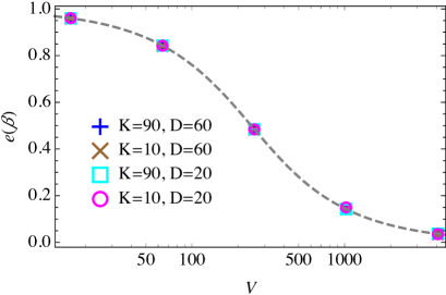
Figure 8: Volume dependence of $e(\beta)$ with $\beta/V=0.01$ for $SU(2)$.

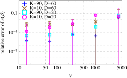
Figure 9: Relative error of the energy density, $|e(\beta)-e_{\rm exact}(\beta)|\,/\,|e_{\rm exact}(\beta)|$, with $\beta/V=0.01$ for $SU(2)$.

We again see good agreements, suggesting the effectiveness of our method. In Figs. 10 and 11, the $K$ and $D$ dependences are shown for $V=64^{2}$ $(\beta=40.96)$, from which we again confirm that the numerical estimates approach the exact value in the limit $K\rightarrow\infty$ and $D\rightarrow\infty$.

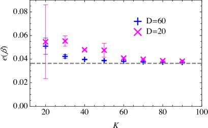
Figure 10: $K$ dependence of $e(\beta)$ with $\beta/V=0.01$ for $SU(2)$.

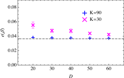
Figure 11: $D$ dependence of $e(\beta)$ with $\beta/V=0.01$ for $SU(2)$.

We can make use of extrapolation to improve the accuracy. Figure 12 shows the $\chi^{2}$ fit to the obtained data with the cost function (3.1) with $f(\beta)$ replaced by $e(\beta)$.

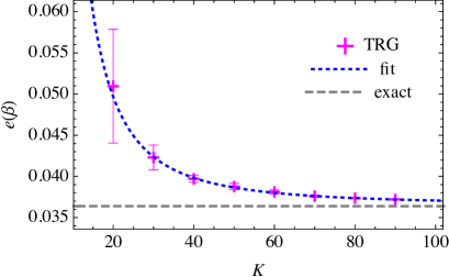
Figure 12: Fitting of the energy densities $e(\beta)$ for various $K$ with $\beta/V=0.01$, $V=64^{2}$ and $D=60$ for $SU(2)$.

The results of the fitting are also given in Table 1.

Figure 13 shows the singular values $\sigma_{A}$ of the initial tensor for $\beta=2$ with $K=90$.

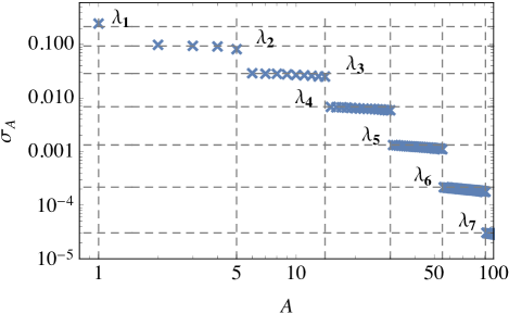
Figure 13: Singular values $\sigma_{A}$ of the initial tensors $T^{(e)}$ [Eq. (2.9)] with $\beta=2$ and $K=90$ for $SU(2)$. Horizontal lines indicate the exact values of $\lambda_{R}(\beta=2)$, and vertical lines the points at which the exact values change discontinuously.

For $SU(2)$, $\lambda_{R}$ in Eq. (2.15) takes the following form (see appendix B):

$$\lambda_{R=\bm{n}}(\beta)=\frac{2}{\beta}\,e^{-\beta}I_{n}(\beta).$$ (3.2)

Here, $\bm{n}$ is the $n$-dimensional irreducible representation of $SU(2)$, and $I_{n}(z)$ is the modified Bessel function of the first kind. According to the discussion in Sec. 2.2, there will be $d_{R}^{2}=n^{2}$ degenerate singular values in the limit $K\rightarrow\infty$ for each representation $R=\bm{n}$. In the figure, we clearly observe this degeneracy even for finite $K$ ($K=90$ here).

Finally, Fig. 14 shows the dependence of the estimate of $f(\beta)$ on the number of $\mathring{G}_{a}$’s with $\beta/V=0.04$, $V=16^{2}$, $D=20$, from which we see that the statistical errors decrease as the number increases.

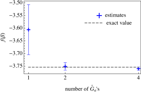
Figure 14: Dependence of the estimate of $f(\beta)$ on the number of $\mathring{G}_{a}$’s ($\beta/V=0.04$, $V=16^{2}$, $K=20$, $D=20$) for $SU(2)$. The statistical errors decrease as the number increases.

This behavior can be understood as follows. We first note that group elements enter the tensor only in the form of the product of two elements, $U_{i}\,U_{j}$, as can be seen from Eq. (2.17). We also note that a better approximation is achieved when the set of $K^{2}$ elements, $\{U_{i}\,U_{j}\}$ $(i,j=1,\ldots,K)$, is closer to the uniform distribution on $G$. As the number of $\mathring{G}_{a}$’s increases, the set $\{U_{i}\,U_{j}\}$ gets more randomly distributed on $G$, which leads to a better estimate of observables with smaller statistical errors.

3.2 $SU(3)$

We make a similar analysis for $SU(3)$ with $\beta/V=0.005$, $V=64^{2}$ and $D=90$. The irreducible representations $R$ of $SU(3)$ are labeled by two nonnegative integers, $R=[q_{1},q_{2}]$ (see appendix B), for which the dimension is given by $d_{R}=(q_{1}+1)(q_{2}+1)(q_{1}+q_{2}+2)/2$. The coefficients $\lambda_{R}(\beta)$ are given by the formula (B.2). One can show that they are ordered as

$$\lambda_{\mathbf{1}}\,>\,\lambda_{\mathbf{3}}=\lambda_{\overline{\mathbf{3}}}\,>\,\lambda_{\mathbf{8}}\,>\,\lambda_{\mathbf{6}}=\lambda_{\overline{\mathbf{6}}}\,>\,\lambda_{\mathbf{15}}=\lambda_{\overline{\mathbf{15}}}\,>\,\lambda_{\mathbf{10}}=\lambda_{\overline{\mathbf{10}}}\,>\,\cdots.$$ (3.3)

In Fig. 15, we plot the free energy densities $f(\beta)$ and the energy densities $e(\beta)$ against various values of $K$.

Figure 15: $K$ dependences of $f(\beta)$ (left panel) and $e(\beta)$ (right panel) with $\beta/V=0.005$, $V=64^{2}$ and $D=90$ for $SU(3)$.

We make the $\chi^{2}$ fit to the obtained data at $K=70,\,80,\ldots,\,120$ again with the scaling ansatz $g(K)\equiv\mu+\alpha K^{-p}$. A similar analysis is performed for $e(\beta)$. The obtained results of the fitting are summarized in Table 2.

	(exact)	$\mu$	$\alpha$	$p$	$\chi^{2}/{\rm DOF}$
$f(\beta)$	-9.4323	$-9.4400^{+0.0019}_{-0.0043}$	$-0.3^{+0.2}_{-1.7}\times 10^{10}$	$5.31^{+0.44}_{-0.01}$	0.21
$e(\beta)$	0.1923	$0.1941^{+0.0017}_{-0.0008}$	$2.2^{+5.6}_{-1.6}\times 10^{10}$	$5.88^{+0.29}_{-0.01}$	1.18

Table 2: Results of the $\chi^{2}$ fit for $SU(3)$.

As for the free energy density $f(\beta)$, we obtain the estimate $\mu=-9.4400^{+0.0019}_{-0.0043}$, which agrees well with the exact value $f_{\rm exact}(\beta)=-9.4323$. As for the energy density $e(\beta)$, we obtain the estimate $\mu=0.1941^{+0.0017}_{-0.0008}$, which also agrees well with the exact value $e_{\rm exact}(\beta)=0.1923$. These good agreements show that our method also works for $SU(3)$.

The singular values of the initial tensor agree with the character expansion coefficients $\lambda_{R}(\beta)$ also for $SU(3)$. Figure 16 shows the singular values $\sigma_{A}$ for $\beta=2$ with $K=120$.

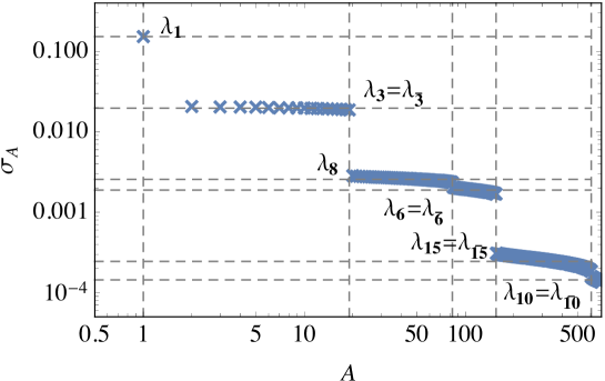
Figure 16: Singular values $\sigma_{A}$ of the initial tensors $T^{(e)}$ [Eq. (2.9)] with $\beta=2$ and $K=120$ for $SU(3)$. Horizontal lines indicate the exact values of $\lambda_{R}(\beta=2)$, and vertical lines the points at which the exact values change discontinuously.

We see that the coefficients are well reproduced with the correct degeneracies, reconfirming the group theoretical structure discussed in Sec. 2.2.

4 Summary and discussion

We have proposed a novel tensor network representation for two-dimensional Yang-Mills theories with arbitrary compact gauge groups, which makes no direct use of the character expansion. The numerical results for $SU(2)$ and $SU(3)$ gauge groups show that our method properly works. Although this paper focuses on pure Yang-Mills theories, it is straightforward to include the dynamical degrees of freedom of fermions and scalar fields into the tensor.

As a future project, it should be important to investigate whether the precision is improved by applying other renormalization algorithms to our tensor network, such as the higher-order tensor renormalization group (HOTRG). It should be also interesting to develop a method to optimally choose group elements from the group manifold, as the Gauss-Hermite quadrature for a field space with flat geometry. The extension of the framework to higher-dimensional Yang-Mills theories should also be one of the next steps to be considered. A study in this direction is now in progress and will be reported elsewhere.

Appendix A Mathematical formulas

In this appendix, we summarize useful formulas for the integration over a compact group $G$.

For a unitary representation $R$ (not necessarily irreducible) with dimension $d_{R}$, we denote the representation matrix of $U\in G$ by $D_{R}(U)=(D^{R}_{rs}(U))$ $(r,s=1,\ldots,d_{R})$ and the character by $\chi_{R}(U)={\rm tr}\,D_{R}(U)$. Note that $\chi_{R}(1)=d_{R}$. Hereafter we use the term “representation” as meaning “representation class”, and fix a representative $R$ for each representation class. Note that for a unitary representation, we have $D^{R}_{rs}(U^{-1})=[D^{R}_{sr}(U)]^{\ast}$ and $\chi_{R}(U^{-1})=[\chi_{R}(U)]^{\ast}$.

We introduce the Haar measure $dU$, which is two-side invariant and normalized:

$$\int dU\,f(g_{1}Ug_{2}) =\int dU\,f(U)\quad(\forall g_{1},\,g_{2}\in G),$$ (A.1)

$$\int dU\,f(U^{-1}) =\int dU\,f(U),$$ (A.2)

$$\int dU\,1 =1.$$ (A.3)

We also introduce the invariant delta function $\delta(U,V)$ associated with the Haar measure:

$$\int dU\,\delta(U,V)\,f(U) =f(V),$$ (A.4)

$$\delta(g_{1}Ug_{2},\,g_{1}Vg_{2}) =\delta(U,V)\quad(\forall g_{1},\,g_{2}\in G),$$ (A.5)

$$\delta(U^{-1},V^{-1}) =\delta(U,V).$$ (A.6)

We write the set of irreducible unitary representations by ${\rm Irrep}=\{R~{}\mbox{: irreducible}\}$. Then, we have the following formula for $R_{1},\,R_{2}\in{\rm Irrep}$:

$$\int dU\,D^{R_{1}}_{r_{1}s_{1}}(U)D^{R_{2}}_{r_{2}s_{2}}(U^{-1})=\frac{\delta_{R_{1}R_{2}}}{d_{R_{1}}}\,\delta_{r_{1}s_{2}}\,\delta_{s_{1}r_{2}},$$ (A.7)

from which we readily obtain the formulas for the integration of characters,

$$\int dU\,\chi_{R_{1}}(g_{1}U)\,\chi_{R_{2}}(U^{-1}g_{2}) =\frac{\delta_{R_{1}R_{2}}}{d_{R_{1}}}\,\chi_{R_{1}}(g_{1}g_{2}),$$ (A.8)

$$\int dU\,\chi_{R}(g_{1}Ug_{2}\,U^{-1}) =\frac{1}{d_{R}}\,\chi_{R}(g_{1})\,\chi_{R}(g_{2}).$$ (A.9)

The characters of irreducible representations $\{\chi_{R}(U)\}$ $(R\in{\rm Irrep})$ form a linear basis of the set of class functions $\{f(U)\}$ that satisfy $f(gUg^{-1})=f(U)$ $(\forall g\in G)$. In particular, as can be easily proved, $\delta(U,1)$ is expanded as $\sum_{R\in{\rm Irrep}}d_{R}\chi_{R}(U)$, and thus we have

$$\delta(U,V)=\sum_{R\in{\rm Irrep}}d_{R}\chi_{R}(UV^{-1})=\sum_{R\in{\rm Irrep}}d_{R}\chi_{R}(VU^{-1}).$$ (A.10)

From this equation readily follows the Peter-Weyl theorem, which states that the infinite dimensional matrix

$$W_{U,A}\equiv\sqrt{d_{R}}\,D^{R}_{rs}(U)\quad[A=(R,r,s)]$$ (A.11)

is unitary:

$$\int dU\,W^{\ast}_{U,A}\,W_{U,A^{\prime}}=\delta_{AA^{\prime}},\quad\sum_{A}W_{U,A}\,W^{\ast}_{U^{\prime},A}=\delta(U,U^{\prime})$$ (A.12)

with $\delta_{AA^{\prime}}\equiv\delta_{RR^{\prime}}\,\delta_{rr^{\prime}}\,\delta_{ss^{\prime}}$ and $\sum_{A}\equiv\sum_{R\in{\rm Irrep}}\sum_{r=1}^{d_{R}}\sum_{s=1}^{d_{R}}$.

Appendix B $\lambda_{R}(\beta)$ for $G=SU(N)$

For $G=SU(N)$, the irreducible representation $R=[q_{1},\ldots,q_{N-1}]$ ($q_{i}\in\mathbb{Z}_{\geq 0}$: Dynkin labels) can be labeled by a Young diagram $Y=(f_{1},f_{2},\ldots,f_{N-1})$ ($f_{1}\geq f_{2}\geq f_{N-1}\geq 0$) with the relations $f_{i}\equiv\sum_{j=i}^{N-1}q_{j}$ (see Fig. 17).

Figure 17: Young diagram for $R=[q_{1},\ldots,q_{N-1}]$.

The dimension $d_{R}$ is given by

$$d_{R}=\Delta(\ell_{1},\ell_{2},\ldots,\ell_{N-1},\ell_{N})/\Delta(N-1,N-2,\ldots,1,0),$$ (B.1)

where $\ell_{i}\equiv f_{i}+N-i$ with $f_{N}\equiv 0$ and $\Delta(x_{1},\ldots,x_{N})\equiv\prod_{i<j}(x_{i}-x_{j})$. One can show that the coefficients $\lambda_{R}(\beta)$ can be expressed as (see, e.g., [44])

$$\lambda_{R}(\beta)=\frac{e^{-\beta}}{d_{R}}\,\sum_{Q\in\mathbb{Z}}\det\bigl{[}I_{f_{j}+i-j+Q}(\beta/N)\bigr{]}\quad[G=SU(N)],$$ (B.2)

where $I_{n}(z)$ are the modified Bessel functions of the first kind.

For $G=SU(2)$, the irreducible representation $R=[q]$ corresponds to the spin $j=q/2$ representation with $d_{R}=q+1=2j+1$, for which the infinite series (B.2) can be summed up to a simple form,

$$\lambda_{R}(\beta)=(2/\beta)\,e^{-\beta}\,I_{2j+1}(\beta)\quad[G=SU(2)].$$ (B.3)

Thus, the free energy density and the energy density can be expressed as

$$f(\beta) ={}\frac{1}{V}\log\Big{[}\sum_{n=1}^{\infty}\Big{(}\frac{2}{\beta}\,e^{-\beta}\,I_{n}(\beta)\Big{)}^{V}\Big{]},$$ (B.4)

$$e(\beta) ={}-\frac{\sum_{n=1}^{\infty}I_{n}^{V-1}(\beta)\big{[}\big{(}I_{n+1}(\beta)+I_{n-1}(\beta)\big{)}/2-I_{n}(\beta)/\beta\big{]}}{\sum_{n=1}^{\infty}I_{n}^{V}(\beta)}+1.$$ (B.5)

Appendix C TN derivation of the exact partition function

The well-known formula (2.20) can be easily derived from the TN representation of the partition function with the infinite dimensional tensor, Eq. (2.19):

$${\mathfrak{T}}^{(1)}_{A_{1}A_{2}A_{3}A_{4}}=\alpha_{1}\,\delta_{R_{1}R_{2}R_{3}R_{4}}\,\delta_{s_{1}s_{2}}\,\delta_{r_{2}s_{3}}\,\delta_{r_{3}r_{4}}\,\delta_{s_{4}r_{1}}.$$ (C.1)

Here, $A_{i}=(R_{i},r_{i},s_{i})$, $\delta_{R_{1}R_{2}\ldots R_{m}}=\delta_{R_{1}R_{2}}\delta_{R_{2}R_{3}}\ldots\delta_{R_{m-1}R_{m}}$, and $\alpha_{n}\equiv\lambda_{R}^{2^{n}}/d_{R}$ $(n=1,2,\ldots)$ are factors located at vertices. Figure 18 shows a graphical representation of ${\mathfrak{T}}^{(1)}$.

Figure 18: Graphical representation of ${\mathfrak{T}}^{(1)}_{A_{1}A_{2}A_{3}A_{4}}$.

It is straightforward to evaluate the value of $Z$ as shown in Fig. 19. Figure 19 (b) is obtained from Fig. 19 (a) where $\alpha_{1}$ is replaced by $\alpha_{1}d_{R}=\lambda_{R}^{2}$ because $d_{R}$ is provided from the inner loop. The final expression is immediately obtained because the remaining tensors in Fig. 19 (b) are diagonal with respect to the $R$ indices [20].

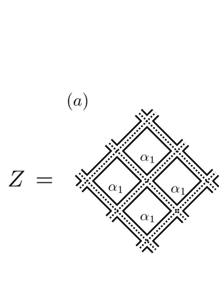
Figure 19: The TN representation of partition function with the infinite dimensional tensor.

Instead, we can use the TRG iterations to evaluate $Z$. Omitting the tensor indices, we write

$${\mathfrak{T}}^{(1)}=\includegraphics[valign={c},width=71.13188pt]{figc2.eps}~{}~{}.$$ (C.2)

Then, we decompose ${\mathfrak{T}}^{(1)}$ in two ways as

$${\mathfrak{T}}^{(1)}=~{}~{}\includegraphics[valign={c},width=79.66771pt]{figc3_a.eps}\quad=\quad\includegraphics[valign={c},width=54.06023pt]{figc3_b.eps}~{}~{},$$ (C.3)

where rank-$3$ tensors are defined in a manner similar to Eq. (C.1). These decompositions correspond to the SVDs given in Fig. 2. With these rank-$3$ tensors, we construct the second tensor as

$${\mathfrak{T}}^{(2)}=~{}~{}\includegraphics[valign={c},width=71.13188pt]{figc4_a.eps}~{}~{}=~{}~{}\includegraphics[valign={c},width=71.13188pt]{figc4_b.eps}~{}~{}.$$ (C.4)

Note that we have not made any truncation. Repeating this procedure, we have the $n$-th tensor

$${\mathfrak{T}}^{(n)}~{}~{}=~{}~{}\includegraphics[valign={c},width=71.13188pt]{figc5.eps}~{}~{},$$ (C.5)

from which the partition function $Z$ with volume $V=2^{n}$ is calculated as

$$Z=\includegraphics[valign={c},width=71.13188pt]{figc6.eps}~{}~{}=\sum_{R}\,\lambda_{R}(\beta)^{V}.$$ (C.6)

References

- [1] H. Niggemann, A. Klumper and J. Zittartz, “Quantum phase transition in spin 3/2 systems on the hexagonal lattice: Optimum ground state approach,” Z. Phys. B 104, 103-110 (1997) [arXiv:cond-mat/9702178 [cond-mat]].
- [2] F. Verstraete and J. I. Cirac, “Renormalization algorithms for quantum-many body systems in two and higher dimensions,” [arXiv:cond-mat/0407066 [cond-mat]].
- [3] M. Levin and C. P. Nave, “Tensor renormalization group approach to 2D classical lattice models,” Phys. Rev. Lett. 99, no.12, 120601 (2007) [arXiv:cond-mat/0611687 [cond-mat.stat-mech]].
- [4] Z. Y. Xie, H. C. Jiang, Q. N. Chen, Z. Y. Weng and T. Xiang, “Second Renormalization of Tensor-Network States,” Phys. Rev. Lett. 103, 160601 (2009) [arXiv:0809.0182 [cond-mat.str-el]].
- [5] Z. C. Gu, F. Verstraete and X. G. Wen, “Grassmann tensor network states and its renormalization for strongly correlated fermionic and bosonic states,” [arXiv:1004.2563 [cond-mat.str-el]].
- [6] Z. Y. Xie, and J. Chen, and M. P. Qin,and J. W. Zhu, and L. P. Yang, and T. Xiang, “Coarse-graining renormalization by higher-order singular value decomposition,” Phys. Rev. B 86, no.4, 045139 (2012) [arXiv:1201.1144 [cond-mat.stat-mech]].
- [7] D. Adachi, T. Okubo and S. Todo, “Anisotropic Tensor Renormalization Group,” Phys. Rev. B 102, no.5, 054432 (2020) [arXiv:1906.02007 [cond-mat.stat-mech]].
- [8] D. Kadoh and K. Nakayama, “Renormalization group on a triad network,” [arXiv:1912.02414 [hep-lat]].
- [9] Y. Shimizu and Y. Kuramashi, “Grassmann tensor renormalization group approach to one-flavor lattice Schwinger model,” Phys. Rev. D 90, no.1, 014508 (2014) [arXiv:1403.0642 [hep-lat]].
- [10] Y. Shimizu and Y. Kuramashi, “Critical behavior of the lattice Schwinger model with a topological term at using the Grassmann tensor renormalization group,” Phys. Rev. D 90, no.7, 074503 (2014) [arXiv:1408.0897 [hep-lat]].
- [11] Y. Shimizu and Y. Kuramashi, “Berezinskii-Kosterlitz-Thouless transition in lattice Schwinger model with one flavor of Wilson fermion,” Phys. Rev. D 97, no.3, 034502 (2018) [arXiv:1712.07808 [hep-lat]].
- [12] N. Butt, S. Catterall, Y. Meurice, R. Sakai and J. Unmuth-Yockey, “Tensor network formulation of the massless Schwinger model with staggered fermions,” Phys. Rev. D 101, no.9, 094509 (2020) [arXiv:1911.01285 [hep-lat]].
- [13] S. Takeda and Y. Yoshimura, “Grassmann tensor renormalization group for the one-flavor lattice Gross–Neveu model with finite chemical potential,” PTEP 2015, no.4, 043B01 (2015) [arXiv:1412.7855 [hep-lat]].
- [14] S. Akiyama, Y. Kuramashi, T. Yamashita and Y. Yoshimura, “Restoration of chiral symmetry in cold and dense Nambu–Jona-Lasinio model with tensor renormalization group,” JHEP 01, 121 (2021) [arXiv:2009.11583 [hep-lat]].
- [15] D. Kadoh, Y. Kuramashi, Y. Nakamura, R. Sakai, S. Takeda and Y. Yoshimura, “Tensor network analysis of critical coupling in two dimensional theory,” JHEP 05, 184 (2019) [arXiv:1811.12376 [hep-lat]].
- [16] D. Kadoh, Y. Kuramashi, Y. Nakamura, R. Sakai, S. Takeda and Y. Yoshimura, “Investigation of complex theory at finite density in two dimensions using TRG,” JHEP 02, 161 (2020) [arXiv:1912.13092 [hep-lat]].
- [17] S. Akiyama, D. Kadoh, Y. Kuramashi, T. Yamashita and Y. Yoshimura, “Tensor renormalization group approach to four-dimensional complex theory at finite density,” JHEP 09, 177 (2020) [arXiv:2005.04645 [hep-lat]].
- [18] S. Akiyama, Y. Kuramashi and Y. Yoshimura, “Phase transition of four-dimensional lattice theory with tensor renormalization group,” [arXiv:2101.06953 [hep-lat]].
- [19] M. Asaduzzaman, S. Catterall and J. Unmuth-Yockey, “Tensor network formulation of two dimensional gravity,” Phys. Rev. D 102, no.5, 054510 (2020) [arXiv:1905.13061 [hep-lat]].
- [20] A. Bazavov, S. Catterall, R. G. Jha and J. Unmuth-Yockey, “Tensor renormalization group study of the non-Abelian Higgs model in two dimensions,” Phys. Rev. D 99, no.11, 114507 (2019) [arXiv:1901.11443 [hep-lat]].
- [21] D. Kadoh, Y. Kuramashi, Y. Nakamura, R. Sakai, S. Takeda and Y. Yoshimura, “Tensor network formulation for two-dimensional lattice = 1 Wess-Zumino model,” JHEP 03, 141 (2018) [arXiv:1801.04183 [hep-lat]].
- [22] H. Kawauchi and S. Takeda, “Tensor renormalization group analysis of CP(N-1) model,” Phys. Rev. D 93, no.11, 114503 (2016) [arXiv:1603.09455 [hep-lat]].
- [23] S. Akiyama and D. Kadoh, “More about the Grassmann tensor renormalization group,” [arXiv:2005.07570 [hep-lat]].
- [24] D. Kadoh, H. Oba and S. Takeda, “Triad second renormalization group,” [arXiv:2107.08769 [cond-mat.str-el]].
- [25] Y. Kuramashi and Y. Yoshimura, “Tensor renormalization group study of two-dimensional U(1) lattice gauge theory with a term,” JHEP 04, 089 (2020) [arXiv:1911.06480 [hep-lat]].
- [26] G. Parisi, “On complex probabilities,” Phys. Lett. B 131, 393 (1983).
- [27] J.R. Klauder, “Coherent State Langevin Equations for Canonical Quantum Systems With Applications to the Quantized Hall Effect,” Phys. Rev. A 29, 2036 (1984).
- [28] G. Aarts, F. A. James, E. Seiler and I. O. Stamatescu, “Adaptive stepsize and instabilities in complex Langevin dynamics,” Phys. Lett. B 687, 154-159 (2010) [arXiv:0912.0617 [hep-lat]].
- [29] J. Nishimura and S. Shimasaki, “New Insights into the Problem with a Singular Drift Term in the Complex Langevin Method,” Phys. Rev. D 92, no.1, 011501 (2015) [arXiv:1504.08359 [hep-lat]].
- [30] E. Witten, “Analytic continuation of Chern-Simons theory,” AMS/IP Stud. Adv. Math. 50, 347-446 (2011) [arXiv:1001.2933 [hep-th]].
- [31] M. Cristoforetti, F. Di Renzo and L. Scorzato, “New approach to the sign problem in quantum field theories: High density QCD on a Lefschetz thimble,” Phys. Rev. D 86, 074506 (2012) [arXiv:1205.3996 [hep-lat]].
- [32] M. Cristoforetti, F. Di Renzo, A. Mukherjee and L. Scorzato, “Monte Carlo simulations on the Lefschetz thimble: Taming the sign problem,” Phys. Rev. D 88, no. 5, 051501(R) (2013) [arXiv:1303.7204 [hep-lat]].
- [33] H. Fujii, D. Honda, M. Kato, Y. Kikukawa, S. Komatsu and T. Sano, “Hybrid Monte Carlo on Lefschetz thimbles - A study of the residual sign problem,” JHEP 1310, 147 (2013) [arXiv:1309.4371 [hep-lat]].
- [34] A. Alexandru, G. Başar, P. F. Bedaque, G. W. Ridgway and N. C. Warrington, “Sign problem and Monte Carlo calculations beyond Lefschetz thimbles,” JHEP 1605, 053 (2016) [arXiv:1512.08764 [hep-lat]].
- [35] M. Fukuma and N. Umeda, “Parallel tempering algorithm for integration over Lefschetz thimbles,” PTEP 2017, no. 7, 073B01 (2017) [arXiv:1703.00861 [hep-lat]].
- [36] A. Alexandru, G. Başar, P. F. Bedaque and N. C. Warrington, “Tempered transitions between thimbles,” Phys. Rev. D 96, no. 3, 034513 (2017) [arXiv:1703.02414 [hep-lat]].
- [37] M. Fukuma, N. Matsumoto and N. Umeda, “Applying the tempered Lefschetz thimble method to the Hubbard model away from half filling,” Phys. Rev. D 100, no. 11, 114510 (2019) [arXiv:1906.04243 [cond-mat.str-el]].
- [38] M. Fukuma, N. Matsumoto and N. Umeda, “Implementation of the HMC algorithm on the tempered Lefschetz thimble method,” [arXiv:1912.13303 [hep-lat]].
- [39] M. Fukuma and N. Matsumoto, “Worldvolume approach to the tempered Lefschetz thimble method,” PTEP 2021, no.2, 023B08 (2021) [arXiv:2012.08468 [hep-lat]].
- [40] M. Fukuma, N. Matsumoto and Y. Namekawa, “Statistical analysis method for the worldvolume hybrid Monte Carlo algorithm,” [arXiv:2107.06858 [hep-lat]].
- [41] Y. Mori, K. Kashiwa and A. Ohnishi, “Toward solving the sign problem with path optimization method,” Phys. Rev. D 96, no.11, 111501 (2017) [arXiv:1705.05605 [hep-lat]].
- [42] Y. Mori, K. Kashiwa and A. Ohnishi, “Application of a neural network to the sign problem via the path optimization method,” PTEP 2018, no.2, 023B04 (2018) [arXiv:1709.03208 [hep-lat]].
- [43] A. Alexandru, P. F. Bedaque, H. Lamm and S. Lawrence, “Finite-Density Monte Carlo Calculations on Sign-Optimized Manifolds,” Phys. Rev. D 97, no.9, 094510 (2018) [arXiv:1804.00697 [hep-lat]].
- [44] J. Carlsson, “Integrals over SU(N),” [arXiv:0802.3409 [hep-lat]].