Green’s functions in quantum mechanics courses

Abstract

Green’s functions in Physics have proven to be a valuable tool for understanding fundamental concepts in different branches, such as electrodynamics, solid-state and many-body problems. In quantum mechanics advanced courses, Green’s functions usually are explained in the context of the scattering problem by a central force. However, their use for more basic problems is not often implemented. The present work introduces Green’s Function in quantum mechanics courses with some examples that can be solved with essential tools. For this, the general aspects of the theory are shown, emphasizing the solution of different fundamental issues of quantum mechanics from this approach. In particular, we introduce the time-independent Green’s functions and the Dyson equation to solve problems with an external potential. As examples, we show the scattering by a Dirac delta barrier, where the reflection and transmission coefficients are found. In addition, the infinite square potential well energy levels, and the local density of states, are calculated.

I Introduction

Green’s function method to solve problems in different areas of physics is done at the undergraduate or graduate level. For example, the usual thing in physics programs is introducing Green’s functions to solve inhomogeneous differential equations, such as the Poisson’s equation, inhomogeneous wave equation, inhomogeneous heat equation [1, 2, 3, 4, 5, 6, 7]. On the other hand, in advanced topics, such as a many-body problem or solid-state physics, Green’s functions are introduced to solve more complex problems that usually require concepts of the second quantization [8, 9, 10, 11, 12, 13, 14, 15, 16]. Moreover, in quantum mechanics courses, the exposition is usually posed in the context of scattering by a central potential, which implies making theoretical developments dependent and independent of time and the use of spherical or cylindrical coordinates [17, 18, 19, 20]. These facts usually lead to Green’s functions in quantum mechanics not being usually exposed in undergraduate courses, which does not allow undergraduate and postgraduate students to be aware of Green’s functions in the context of quantum mechanics. However, sometimes it involves realizing more elaborate calculations or using the complex variable [21, 22, 23, 24, 25, 26, 27, 28, 29, 30, 31], and other works show methods to find the Green’s function in specific problems of quantum mechanics [28, 32, 33]. In this work, we make an approach that can help introduce the concept and service of Green’s function in intermediate or advanced quantum mechanics courses. First, we present the formalism of Green’s functions and how we can use it for the time-independent Schrödinger equation. Later, we explain Green’s function of a free particle and derive the Dyson equation when the system is perturbed with a scalar potential. In particular, we consider a Dirac delta potential, where we find the Green’s function for both reflection and transmission coefficients. Likewise, it illustrates how to find the Green’s function of an infinite square potential well, and from it, we can calculate the spectrum of energy and the local density of states (LDOS).

II Green’s functions for the Schrödinger and Dyson equations.

Before starting with the implementation of the Green’s function for the Schrödinger equation, let us do a brief review of the Green’s function associated with a linear operator $\hat{L}_{x}$ in the $x$ coordinate representation,

$$\left(\lambda-\hat{L}_{x}\right)\phi\left(x\right)=f\left(x\right).$$ (1)

We wish to find the inverse operator $\left(\lambda-\hat{L}\right)^{-1}$, such that $\phi=\left(\lambda-\hat{L}\right)^{-1}f$. The nucleus of an integral $G(x,x^{\prime})$ will represent this inverse operator, defined as

$$\left(\lambda-\hat{L}\right)_{x,x^{\prime}}^{-1}=G(x,x^{\prime}),$$ (2)

such that the integral solution of the equation (1) can write, as

$$\phi(x)=\int G(x,x^{\prime})f(x^{\prime})dx^{\prime},$$ (3)

where $G(x,x^{\prime})$ is known as Green’s function (GF). Now let us derive the differential equation that satisfies $G(x,x^{\prime})$, applying the operator $\lambda-\hat{L}$ to the equation (3), in this manner

$$\left(\lambda-\hat{L}_{x}\right)\phi(x) = \int\left(\lambda-\hat{L}_{x}\right)G(x,x^{\prime})f(x^{\prime})dx^{\prime}$$ (4)

$$= f(x).$$ (5)

Therefore $G(x,x^{\prime})$ must satisfy

$$\left(\lambda-\hat{L}_{x}\right)G(x,x^{\prime})=\delta(x-x^{\prime}).$$ (6)

Furthermore, Green’s function coordinate representation satisfies an inhomogeneous differential equation with $f(x)=\delta(x-x^{\prime})$. From the solution of Eq. (6) we can solve the equation (3). Using the inverse operator notation gives that

$$...\left(\lambda-\hat{L}\right)^{-1}=\int...G(x,x^{\prime})dx^{\prime}.$$ (7)

In such a way,

$$\left(\lambda-\hat{L}_{x}\right)\left(\lambda-\hat{L}_{x}\right)^{-1}=\int\delta(x-x^{\prime})dx=1.$$ (8)

Now, we consider the time-independent Schrödinger equation,

$$H_{0}\left(\mathbf{r}\right)\psi(\mathbf{r})=E\psi_{0}(\mathbf{r}),$$ (9)

with

$$H_{0}\left(\mathbf{r}\right)=-\dfrac{\hbar^{2}}{2m}\nabla^{2}+V_{0}(\mathbf{r}).$$ (10)

Here, the subscript $0$ refers to the potential $V_{0}$. Even if this equation is homogeneous; we can define the associated Green’s function, as

$$\left(E-H_{0}\left(\mathbf{r}\right)\right)g(\mathbf{r,r}^{\prime})=\delta(\mathbf{r-r}^{\prime}),$$ (11)

whose solution we can write as,

$$g(\mathbf{r,r}^{\prime})=\left(E-H_{0}\left(\mathbf{r}\right)\right)^{-1}\delta(\mathbf{r-r}^{\prime}).$$ (12)

The function $g(\mathbf{r,r}^{\prime})$ depends on $E$, which does not explicitly notice. To the value of $E$, we usually add or subtract a small imaginary part, $E\rightarrow E\pm i\eta$, thus $g(\mathbf{r,r}^{\prime})$ has no poles on the real axis when $E$ matches a set energy value of the system. When we add $i\eta$, the Green’s function is called retarded ($r$) and for $-i\eta$ advanced ($a$), see note . In the following, only when explicitly needed we will refer to the advanced or retarded Green’s function.

The Green’s function $g(\mathbf{r,r}^{\prime})$ becomes significant when to the Hamiltonian $H_{0}\left(\mathbf{r}\right)$ we add a potential $V\left(\mathbf{r}\right)$, which involves solving

$$\left(H_{0}\left(\mathbf{r}\right)+V\left(\mathbf{r}\right)\right)\psi(\mathbf{r})=E\psi(\mathbf{r}),$$ (13)

so, we can express it as

$$\left(E-H_{0}\left(\mathbf{r}\right)\right)\psi(\mathbf{r})=V\left(\mathbf{r}\right)\psi(\mathbf{r}).$$ (14)

We can see this equation as an “inhomogeneous” Schrödinger equation, where the external source is given by $f\left(\mathbf{r}\right)=V\left(\mathbf{r}\right)\psi(\mathbf{r})$, we start from the fact that we know $g(\mathbf{r,r}^{\prime})$, and then we can write the solution for $\psi(\mathbf{r})$ as

$$\psi(\mathbf{r})=\psi_{0}\left(\mathbf{r}\right)+\int d\mathbf{r}^{\prime}g\left(\mathbf{r},\mathbf{r}^{\prime}\right)V\left(\mathbf{r}^{\prime}\right)\psi(\mathbf{r}^{\prime}).$$ (15)

This is an integral equation to find $\psi(\mathbf{r})$ from $g\left(\mathbf{r},\mathbf{r}^{\prime}\right)$ however, it is possible to express $\psi(\mathbf{r})$ more directly from the Green’s function of the perturbed system, to define $G(\mathbf{r,r}^{\prime})$, as

$$\left(E-H\right)G(\mathbf{r,r}^{\prime})=\delta(\mathbf{r-r}^{\prime}),$$ (16)

with $H=H_{0}\left(\mathbf{r}\right)+V\left(\mathbf{r}\right)$. Using Eq.(11) to write $\delta(\mathbf{r-r}^{\prime})$, $G(\mathbf{r,r}^{\prime})$ can be written as

$$G(\mathbf{r,r}^{\prime}) = \left(E-H\left(\mathbf{r}\right)\right)^{-1}\delta(\mathbf{r-r}^{\prime})$$ (17)

$$= \left(E-H\left(\mathbf{r}\right)\right)^{-1}\left(E-H_{0}\left(\mathbf{r}\right)\right)g(\mathbf{r,r}^{\prime})$$

$$= \left(E-H\left(\mathbf{r}\right)\right)^{-1}\left(E-H\left(\mathbf{r}\right)+V\left(\mathbf{r}\right)\right)g(\mathbf{r,r}^{\prime})$$

$$= g(\mathbf{r,r}^{\prime})+\left(E-H\left(\mathbf{r}\right)\right)^{-1}V\left(\mathbf{r}\right)g(\mathbf{r,r}^{\prime}).$$

From the inverse operator notation (7) for $\left(E-H\left(\mathbf{r}\right)\right)^{-1}$, $G(\mathbf{r,r}^{\prime})$ is

$$G(\mathbf{r,r}^{\prime})=g(\mathbf{r,r}^{\prime})+\int d\mathbf{r}_{1}G(\mathbf{r,r}_{1})V\left(\mathbf{r}_{1}\right)g(\mathbf{r}_{1}\mathbf{,r}^{\prime}).$$ (18)

This result is called the Dyson equation, and it allows us to express the Green’s function of the perturbed system in terms of the Green’s function of the unperturbed system. Similarly, we can find $\psi\left(\mathbf{r}\right)$ from $G(\mathbf{r,r}^{\prime})$, for this we do

$$E\psi_{0}(\mathbf{r})-H_{0}(\mathbf{r})\psi_{0}(\mathbf{r}) = 0$$

$$\left(E-H(\mathbf{r})\right)\psi_{0}(\mathbf{r}) = -V(\mathbf{r})\psi_{0}(\mathbf{r}),$$ (19)

in this case, the external source is given by $f\left(\mathbf{r}\right)=-V\left(\mathbf{r}\right)\psi_{0}(\mathbf{r})$, and using (16), we can express

$$\psi_{0}(\mathbf{r})=\psi(\mathbf{r})-\int G(\mathbf{r},\mathbf{r}^{\prime})V(\mathbf{r})\psi_{0}(\mathbf{r})d\mathbf{r}^{\prime},$$ (20)

where we use the solution of equation (19) for $V\left(\mathbf{r}\right)=0$ that is $\psi(\mathbf{r})$, we found

$$\psi(\mathbf{r})=\psi_{0}(\mathbf{r})+\int G(\mathbf{r},\mathbf{r}^{\prime})V(\mathbf{r}^{\prime})\psi_{0}(\mathbf{r}^{\prime})d\mathbf{r}^{\prime},$$ (21)

which allows us to find the quantum state of the perturbed system from the unperturbed wave function and the Green’s function $G$ that is found from the unperturbed Green’s function $g$ solving the equation (18).

III Dirac delta potential in one dimension.

As a first example, we consider the Schrödinger equation for a particle in one dimension with a potential of the form

$$V\left(x\right)=U_{0}\delta\left(x\right),$$ (22)

it can model a thin potential barrier that couples two regions of a material, such as two metals separated by an oxide layer. Here, $U_{0}=a_{0}V_{0}$, where $a_{0}$ is the width of the barrier and $V_{0}$, the height (see FIG. 1), is a parameter that gives us the characteristic of how strong the barrier is. Dyson’s equation in terms of the coordinates $x$ and $x^{\prime}$, is written as

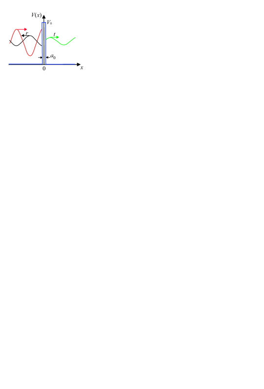
Figure 1: Potential barrier of width $a_{0}$ and height $V_{0}$, when $a_{0}\rightarrow 0$ and $V_{0}\rightarrow\infty$ but $a_{0}V_{0}\rightarrow U_{0}$ the potential can be modelled as $V\left(x\right)=U_{0}\delta\left(x\right)$. The red line illustrates the incoming wave, and the black and green lines are the reflected ($r$) and transmitted ($t$) waves, respectively.

$$G(x,x^{\prime})=g(x,x^{\prime})+\int g(x,x_{1})V\left(x_{1}\right)G(x_{1},x^{\prime})dx_{1},$$ (23)

replacing the potential $V\left(x\right)$, we get

$$G(x,x^{\prime})=g(x,x^{\prime})+U_{0}g(x,0)G(0,x^{\prime}).$$ (24)

From this equation we can find $G(0,x^{\prime})$

$$G(0,x^{\prime}) = g(0,x^{\prime})+U_{0}g(0,0)G(0,x^{\prime})$$

$$G(0,x^{\prime}) = \left[1-U_{0}g(0,0)\right]^{-1}g(0,x^{\prime}),$$ (25)

and replacing in (24), we get

$$G(x,x^{\prime})=g(x,x^{\prime})+U_{0}g(x,0)\left[1-U_{0}g(0,0)\right]^{-1}g(0,x^{\prime}).$$ (26)

The unperturbed function $g(x,x^{\prime})$ corresponds to an infinite one-dimensional system. In Appendix A we show the method of the asymptotic solutions to calculate the Green’s function in one dimension and, we applied this to find the GF of the free particle, which is given by

$$g(x,x^{\prime})=Ae^{ik\left|x-x^{\prime}\right|},$$ (27)

with

$$k=\sqrt{2mE/{\hbar^{2}}},A=-i\frac{m}{\hbar^{2}k}.$$ (28)

Replacing $g(x,x^{\prime})$ in Eq. (26) we obtain,

$$G(x,x^{\prime})=A\left(e^{ik\left|x-x^{\prime}\right|}+U_{0}Ae^{ik\left(\left|x\right|+\left|x^{\prime}\right|\right)}\left[1-U_{0}A\right]^{-1}\right).$$ (29)

Defining $Z$ as the strength of the barrier

$$Z=\dfrac{m}{\hbar^{2}k}U_{0},$$ (30)

we get,

$$G(x,x^{\prime})=A\left(e^{ik\left|x-x^{\prime}\right|}-\frac{iZ}{1+iZ}e^{ik\left(\left|x\right|+\left|x^{\prime}\right|\right)}\right).$$ (31)

The first term comes from the Green’s function of the homogeneous system, and the second, from particle interaction with the potential, which breaks the homogeneity of the system. Now to find the perturbed wave function, we use (21), with which

$$\psi(x) = \psi_{0}\left(x\right)+\int G(x,x^{\prime})U_{0}\delta(x^{\prime})\psi_{0}(x{{}^{\prime}})dx^{\prime}$$ (32)

$$= \psi_{0}\left(x\right)+G(x,0)U_{0}\psi_{0}(0).$$

If we assume an incident wave from the left, the unperturbed wave function is

$$\psi_{0}\left(x\right)=ae^{ikx},$$ (33)

with $a$ the amplitude of the wave. From (31), we can express

$$G(x,0)=Ae^{ik\left|x\right|}\left(\frac{1}{1+iZ}\right),$$ (34)

Using (32), (33) and (34), we obtain

$$\psi(x)=a\left(e^{ikx}-e^{ik\left|x\right|}\frac{iZ}{1+iZ}\right).$$ (35)

We can write explicitly to the left and right of the barrier the wave function as

$$\psi(x)=\left\{\begin{array}[]{cr}a\left(e^{ikx}-e^{-ikx}\frac{iZ}{1+iZ}\right),&x<0\\ ae^{ikx}\frac{1}{1+iZ},&x>0.\end{array}\right.$$ (36)

From here, we can see that the amplitudes of reflection ($r$), and transmission ($t$) are

$$r=\frac{-iZ}{1+iZ},\hskip 5.69046ptt=\frac{1}{1+iZ},$$ (37)

in such a way that the reflection and transmission coefficients are

$$R=\left|r\right|^{2}=\frac{Z^{2}}{1+Z^{2}},\;T=\left|t\right|^{2}=\frac{1}{1+Z^{2}}.$$ (38)

These coefficients satisfy that $R^{2}+T^{2}=1$. These are illustrated in FIG. 2.
Let us go back to Green’s function and analyze the case of an infinite barrier, for which we do $U_{0},Z\rightarrow\infty$

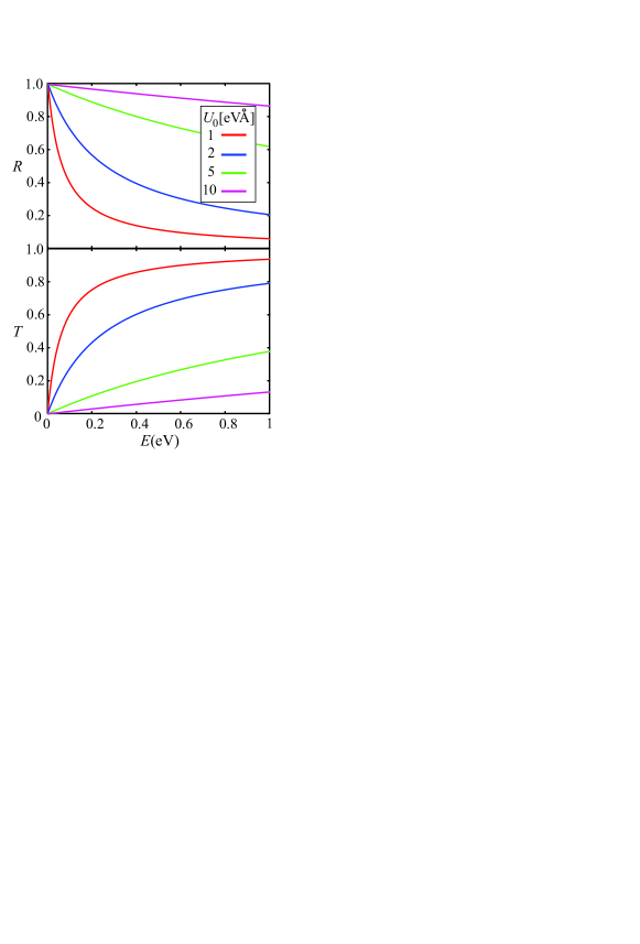
Figure 2: Reflection and transmission coefficients as a function of the energy for different values of $U_{0}$. the units of $U_{0}$ are $eV\r{A}$ that corresponds to an insulating barrier for a typical metal-oxide-metal system.

$$G(x,x^{\prime})=A\left(e^{ik\left|x-x^{\prime}\right|}-e^{ik\left(\left|x\right|+\left|x^{\prime}\right|\right)}\right).$$ (39)

This Green’s function corresponds to that of a semi-finite medium to left or right at $x=0,$ and it will be used in the next section.

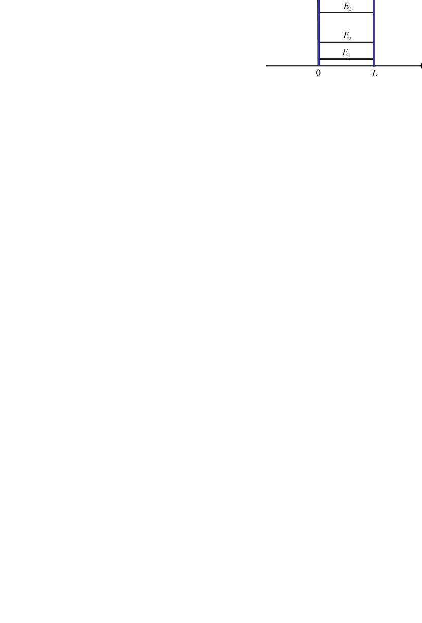
Figure 3: Potential well, formed from two Dirac functions at $x=0$ and $x=L$, with $U_{0}$ and $U_{1}$ as parameters. When $U_{0/1}\rightarrow\infty$, we obtain an infinite square potential well.

IV Green’s function for a quantum potential well.

We are going to find the Green’s function of an infinite potential well; see FIG. 3. To do this, we start from the Green’s function of the semi-infinite medium with $x>0$ and place an additional potential at $x=L$

$$V\left(x\right)=U_{1}\delta(x-L),$$ (40)

with $U_{1}=a_{1}V_{1}$, $a_{1}$ being the width of the additional barrier and $V_{1}$ its height. For the Dyson equation the unperturbed Green’s function is given by (39) with $x,x^{\prime}>0$ and denoted as $g(x,x^{\prime})$

$$g(x,x^{\prime})=A\left(e^{ik\left|x-x^{\prime}\right|}-e^{ik\left(x+x^{\prime}\right)}\right).$$ (41)

Proceeding similarly to the case of a barrier we have,

$$G(x,x^{\prime})=g(x,x^{\prime})+U_{1}g(x,L)\left[1-U_{1}g(L,L)\right]^{-1}g(L,x^{\prime}),$$ (42)

at the limit of $U_{1}\rightarrow\infty$, we obtain the Green’s function from an infinite square potential well as

$$G(x,x^{\prime})=g(x,x^{\prime})-g(x,L)\left[g(L,L)\right]^{-1}g(L,x^{\prime}).$$ (43)

For $x<x^{\prime}$ explicitly replacing (41), we get

$$G(x,x^{\prime})=-i\dfrac{m}{\hbar^{2}k}\frac{\left(e^{-ikx}-e^{ikx}\right)\left(e^{ikx^{\prime}}-e^{-ik(x^{\prime}-2L)}\right)}{1-e^{i2kL}}.$$ (44)

From the poles of the Green’s function, see Appendix $B$, we find that the energy spectrum is given by

$$e^{i2kL}=1,$$ (45)

therefore

$$\;k=\dfrac{n\pi}{L},\;E_{n}=\dfrac{\hbar^{2}\pi^{2}}{2mL^{2}}n^{2}.$$ (46)

Which coincides with the eigenstates of an infinite square potential well. To starting from $G(x,x^{\prime})$, we can find the local density of states, see Appendix $B$,

$$\rho\left(x,E\right)=-\frac{1}{\pi}\text{Im}\left[G^{r}(x,x,E)\right],$$ (47)

remembering that $G^{r}(x,x,E)=G(x,x,E+i\eta)$ is the retarded Green’s function. The figure 4 illustrates the LDOS and the density of states which is defined as

$$N\left(E\right)=\int dx\rho\left(x,E\right).$$ (48)

Then, when $E$ coincides with an eigenvalue of the system, $N(E)$ has a maxima, and $\rho(x,E)$ is proportional to the probability density corresponding to that eigenvalue.

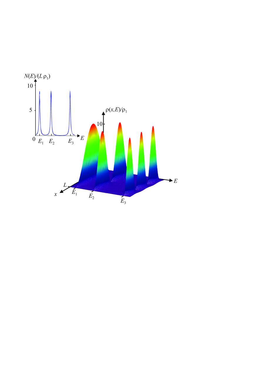
Figure 4: Local density of states for an infinite square potential well, as a function of $x$ and energy. The inset shows the density of states, where we can observe that $N(E)$ is maximal when $E=E_{n}$. Here, $\rho_{1}=1/(2E_{1}L)$ and the integral of $N(E)dE$ for each peak is 1.

V Conclusions

In this work, we have introduced the time-independent Green’s Function for the Schrödinger equation. Also, we have derived the Dyson Equation to solve an “inhomogeneous” Schrödinger equation when an external potential perturbs the system. As a first example for applying the Dyson Equation with unbounded states, we solve a potential modelled by a Dirac delta function, where we find the Green’s function and the wave function, such as the reflection and transmission coefficients. To study bound states, we solve the infinite square potential well and find the GF, the energy spectrum, and local density of states. We showed the method of the asymptotic solutions to calculate the Green’s function in one dimension and applied this to find the GF of the free particle. The methods to find Green’s functions and examples show how to introduce this concept in quantum mechanics courses.

Appendix A Calculation of Green’s function using asymptotic solutions

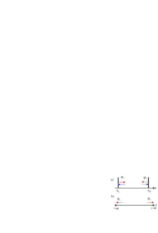
Figure 5: Schematic representation of the asymptotic functions, the arrows illustrate the group velocity of each wave travelling in different directions. a) For a semi-infinite system with an edge at $x_{L}$ or $x_{R}$ and the function in each case is a linear combination of incoming (blue arrows) and outgoing (red arrows) plane waves. b) For an infinite system where $x_{R/L}\rightarrow\pm\infty$ and the functions are outgoing plane waves.

One method to find the Green’s function in one dimension is to use the asymptotic solutions of the differential equation. As $G(x,x^{\prime})$ fulfills the homogeneous equation for $x\neq x^{\prime}$, we can write

$$G(x,x^{\prime})=\left\{\begin{array}[]{cl}A\varphi_{<}(x)\varphi_{>}(x^{\prime}),&x<x^{\prime}\\ A^{\prime}\varphi_{<}(x^{\prime})\varphi_{>}(x),&x>x^{\prime}.\end{array}\right.$$ (49)

The functions $\varphi_{<}({x})$ and $\varphi_{>}({x})$ are solutions of the Schrödinger equation that satisfy the boundary conditions left or right respectively. For example, $\varphi_{<}(x_{L})=0$, $\varphi_{>}(x_{R})=0$, $x_{L}<x_{R}$, see FIG. 5a. The product $\varphi_{<}(x)\varphi_{>}(x^{\prime})$ assures us that $G(x,x^{\prime})$ satisfies the Schrödinger equation for both the operator $H(x)$ as for $H({x}^{\prime})$. The constants $A$ and $A^{\prime}$ are determined from the boundary conditions at $x=x^{\prime}$. Integrating the differential equation

$$\left(E-V(x)+\dfrac{\hbar^{2}}{2m}\dfrac{d^{2}}{dx^{2}}\right)G(x,x^{\prime})=\delta(x-x^{\prime})$$ (50)

between $x^{\prime}-\epsilon$ and $x^{\prime}+\epsilon$, we get

$$\int\limits_{x`-\varepsilon}^{x`+\varepsilon}dx\left(E-V(x)+\dfrac{\hbar^{2}}{2m}\dfrac{d^{2}}{dx^{2}}\right)G(x,x^{\prime})=\int\limits_{x`-\varepsilon}^{x`+\varepsilon}dx\delta(x-x^{\prime}).$$ (51)

Taking the limit when $\epsilon\rightarrow 0$, we find that

$$\dfrac{dG(x,x+\varepsilon)}{dx}-\dfrac{dG(x,x-\varepsilon)}{dx}=\dfrac{2m}{\hbar^{2}},$$ (52)

integrating again

$$G(x,x+\varepsilon)=G(x,x-\varepsilon).$$ (53)

Replacing the assumption (49) in the boundary conditions of (52) and (53), we obtain

$$\centering{A\varphi_{<}(x)\varphi_{>}(x)}{=A^{\prime}\varphi_{<}(x)\varphi_{>}(x)}\@add@centering$$

$${A^{\prime}\varphi_{<}(x)\dfrac{d\varphi_{>}(x)}{dx}-A^{\prime}\dfrac{d\varphi_{<}(x)}{dx}\varphi_{>}(x)}{=\dfrac{2m}{\hbar^{2}}}$$ .

Solving these equations

$$A=A^{\prime}=\dfrac{2m}{\hbar^{2}W},$$ (54)

where $W$ is the Wronskian,

$$W=\varphi_{<}(x)\dfrac{d\varphi_{>}(x)}{dx}-\dfrac{d\varphi_{<}(x)}{dx}\varphi_{>}(x),$$ (55)

which is independent of $x$, $dW/dx=0$. With this, we finally write

$$G(x,x^{\prime})=\dfrac{2m}{\hbar^{2}W}\left\{\begin{array}[]{l}{\varphi_{<}(x)\varphi_{>}(x^{\prime}),\;x<x^{\prime}}\\ {\varphi_{<}(x^{\prime})\varphi_{>}(x),\;x>x^{\prime}.}\end{array}\right.$$ (56)

As an example, we consider the free particle case which the asymptotic solutions are, see FIG. 5b

$$\varphi_{<}(x) = e^{-ikx},$$

$$\varphi_{>}({x}) = e^{ik{x}},$$

with $k=\sqrt{2mE/\hbar^{2}}$. The wave function $\varphi_{<}(x)$ describes an electron that propagates to the left and $\varphi_{>}(x)$ one that propagates to the right, using (55)

$$W=ike^{-ikx}e^{ik{x}}+ike^{-ikx}e^{ik{x}}=2ik,$$

and from Eq. (56) we obtain

$$G(x,x^{\prime})=-i\dfrac{m}{\hbar^{2}k}\left\{\begin{array}[]{ll}e^{-ikx}e^{ik{x}^{\prime}},&x<x^{\prime}\\ e^{-ikx^{\prime}}e^{ik{x}},&x>x^{\prime},\end{array}\right.$$ (57)

which can be written as

$$G(x,x^{\prime})=-i\dfrac{m}{\hbar^{2}k}e^{ik|x-x^{\prime}|}.$$ (58)

Appendix B Density of states

For a system, such as a metal, in which the electronic energy levels form a quasi-continuum, a function of great importance is the density of states $N(E)$, where $N(E){dE}$ is defined as the number of states with energies between $E$ and $E+dE$. We are going to show that the density of states can be expressed in terms of a Green’s function, then we are going to find an expression of the GF in terms of the eigenfunctions of the Hamiltonian $H$, which we assume orthonormal and complete

$$\int d\mathbf{r}\varphi_{n}\left(\mathbf{r}\right)\varphi_{m}^{\ast}\left(\mathbf{r}\right) = \delta_{n,m},$$ (59)

$$\;\sum\limits_{n}\varphi_{n}\left(\mathbf{r}\right)\varphi_{n}^{\ast}\left(\mathbf{r}^{\prime}\right) = \delta\left(\mathbf{r-r}^{\prime}\right).$$ (60)

Assuming a solution of the form

$$G\left(\mathbf{r},\mathbf{r}^{\prime}\right)=\sum\limits_{n}d_{n}\varphi_{n}\left(\mathbf{r}\right)\varphi_{n}^{\ast}\left(\mathbf{r}^{\prime}\right),$$ (61)

we replace it in

$$\left(E-H\right)G\left(\mathbf{r},\mathbf{r}^{\prime}\right)=\delta\left(\mathbf{r-r}^{\prime}\right),$$ (62)

and using the completeness condition (60), we obtain

$$\sum\limits_{n}d_{n}\left(E-E_{n}\right)\varphi_{n}\left(\mathbf{r}\right)\varphi_{n}^{\ast}\left(\mathbf{r}^{\prime}\right)=\sum\limits_{n}\varphi_{n}\left(\mathbf{r}\right)\varphi_{n}^{\ast}\left(\mathbf{r}^{\prime}\right)$$ (63)

in this way, $d_{n}=\left(E-E_{n}\right)^{-1},$ and therefore

$$G\left(\mathbf{r},\mathbf{r}^{\prime}\right)=\sum\limits_{n}\frac{\varphi_{n}\left(\mathbf{r}\right)\varphi_{n}^{\ast}\left(\mathbf{r}^{\prime}\right)}{E-E_{n}}.$$ (64)

To avoid singularity at $E=E_{n}$ we define the retarded Green’s function, as

$$G^{r}\left(\mathbf{r},\mathbf{r}^{\prime}\right)=\sum\limits_{n}\frac{\varphi_{n}\left(\mathbf{r}\right)\varphi_{n}^{\ast}\left(\mathbf{r}^{\prime}\right)}{E-E_{n}+i\eta},$$ (65)

with $\eta$ an infinitesimal part tending to zero, $\eta\rightarrow 0.$ Here we see that $G^{r}$ has the property that it diverges when $E$ coincides with an eigenvalue of system energy $E_{n}$. This property allows us to find the energy spectrum from the poles of the Green’s function. Taking $\mathbf{r}^{\prime}=\mathbf{r}$ and making the integral in $d\mathbf{r}$, we get

$$\int d\mathbf{r}G^{r,r}\left(\mathbf{r,}E\right)=\sum\limits_{n}\dfrac{1}{E-E_{n}+i\eta}.$$ (66)

This sum is usually expressed by an integral with the definition of the density of states $N(E)$

$$\int d\mathbf{r}G^{r}\left(\mathbf{r},\mathbf{r},E\right)=\int dE^{\prime}\dfrac{N(E^{\prime})}{E-E^{\prime}+i\eta},$$ (67)

with

$$N(E)=\sum\limits_{n}\delta\left(E-E_{n}\right).$$ (68)

The denominator in (67)  can be written as

$$\frac{1}{E-E^{\prime}+i\eta} = \frac{E-E^{\prime}-i\eta}{\left(E-E^{\prime}\right)^{2}+\eta^{2}}$$

$$= \frac{E-E^{\prime}}{\left(E-E^{\prime}\right)^{2}+\eta^{2}}-i\pi\frac{1}{\pi}\frac{\eta}{\left(E-E^{\prime}\right)^{2}+\eta^{2}}.$$

When $\eta\rightarrow 0$ the first term corresponds to the Cauchy principal part and the second to a Dirac delta function,

$$\frac{1}{E-E^{\prime}+i\eta}=P\frac{1}{E-E^{\prime}}-i\pi\delta\left(E-E^{\prime}\right).$$ (69)

With this, the equation (67) is

$$\int d\mathbf{r}G^{r}\left(\mathbf{r},\mathbf{r}\right)=P\int dE^{\prime}\dfrac{N(E^{\prime})}{E-E^{\prime}}-i\pi N\left(E\right).$$ (70)

Since the principal part is real, we have to

$$N\left(E\right)=-\frac{1}{\pi}\text{Im}\int d\mathbf{r}G^{r}\left(\mathbf{r},\mathbf{r},E\right).$$ (71)

We define the local density of states $\rho\left(\mathbf{r},E\right)$ from

$$N\left(E\right)=\int d\mathbf{r}\rho\left(\mathbf{r},E\right),$$ (72)

with

$$\rho\left(\mathbf{r},E\right)=-\frac{1}{\pi}\text{Im}\left[G^{r}\left(\mathbf{r},\mathbf{r},E\right)\right].$$ (73)

Using the equations (65), (68), and (69) $\rho\left(\mathbf{r},E\right)$ can be expressed as

$$\rho\left(\mathbf{r},E\right)=\sum\limits_{n}\left|\varphi_{n}\left(\mathbf{r}\right)\right|^{2}\delta\left(E-E_{n}\right),$$ (74)

which shows that the local density of states is proportional to the probability density.

Appendix C Challenge Problems

C.1 Problem: Resonances in a double barrier potential.

Consider a double barrier potential, which is modelled by two Dirac delta barriers

$$V\left(x\right)=U_{a}\delta(x)+U_{b}\delta(L).$$ (75)

Show that by replacing this potential in Dyson’s equation, we obtain

$$G(x,x^{\prime})=g(x,x^{\prime})+U_{a}G(x,0)g(0,x^{\prime})+U_{b}G(x,L)g(L,x^{\prime}).$$ (76)

From this equation, two equations can be obtained that connect the functions $G(x,0)$ and $G(x,L)$. From them, find that

$$G(x,x^{\prime}) = \frac{A}{1-r_{a}r_{b}e^{2ikL}}\{\left(1-r_{a}r_{b}e^{2ikL}\right)e^{ik|x-x^{\prime}|}$$ (77)

$$+ r_{a}e^{ik|x|}\left(e^{ik|x^{\prime}|}+r_{b}e^{ikL}e^{ik|L-x^{\prime}|}\right)$$

$$+ r_{b}e^{ik|x-L|}\left(e^{ik|L-x^{\prime}|}+r_{a}e^{ikL}e^{ik|x^{\prime}|}\right)\},$$

with $k=\sqrt{2mE/\hbar^{2}}$, $r_{i}$ and $t_{i}$ the amplitudes of reflection and transmission for each barrier, $i=a,b$, given by

$$r_{i} = \frac{-iZ_{i}}{1+iZ_{i}}=\left|r_{i}\right|e^{i\alpha_{i}},$$ (78)

$$t_{i} = \frac{1}{1+iZ_{i}}=\left|t_{i}\right|e^{i\beta_{i}},$$ (79)

where $Z_{i}$ is the strength for each barrier

$$Z_{i}=\dfrac{m}{\hbar^{2}k}U_{i}.$$ (80)

From the Green’s function calculate the wave function using the equation (21), and assuming an incident wave $\psi_{0}(x)=e^{ikx}$. For $x>L$, get

$$\psi(x)=te^{ikx},$$ (81)

with $t$ the transmission amplitude of the double barrier potential, given by

$$t=\frac{t_{a}t_{b}}{1-r_{a}r_{b}e^{2ikL}}.$$ (82)

In the symmetric case $Z_{a}=Z_{b},$ show that

$$t=\frac{\left|t_{a}\right|^{2}e^{2i\beta_{a}}}{1-\left|r_{a}\right|^{2}e^{2ikL+2i\alpha_{a}}},$$ (83)

when

$$e^{2ikL+2i\alpha_{a}}=1,$$ (84)

find that

$$t=\frac{t_{a}^{2}}{1-\left|r_{a}\right|^{2}}=e^{2i\beta_{a}},$$ (85)

thus, the transmission coefficient is one

$$T=\left|e^{2i\beta_{a}}\right|^{2}=1.$$ (86)

That constitutes resonant tunnelling through quasi-bound states from the well. Plot the transmission coefficient for different values of $Z$ and observe how the width of each resonance depends on $Z$.

C.2 Problem: Green’s function of an infinite quantum potential well by asymptotic solutions.

Consider an infinite potential well with boundaries at $x=$ 0, and $x=L$. The asymptotic solutions, are

$$\varphi_{<}(x) = e^{-ikx}+ae^{ikx},$$

$$\varphi_{>}({x}) = e^{ik{x}}+be^{-ik{x}},$$

with $a$ and $b$ the reflection amplitudes. From the boundary conditions of the wave functions $\varphi_{<}$ at $x=0$, and $\varphi_{>}$ at $x=L$ for “fixed endpoints ” $\varphi_{<}(0)=\varphi_{>}(L)=0$, show that

$$a=-1,b=-e^{i2kL}.$$ (87)

From $\varphi_{<}(x)$ and $\varphi_{>}(x)$ obtain that

$$G(x,x^{\prime})=-i\dfrac{m}{\hbar^{2}k}\frac{\left(e^{-ikx}-e^{ikx}\right)\left(e^{ikx^{\prime}}-e^{-ik(x^{\prime}-2L)}\right)}{(1-e^{i2kL})},$$ (88)

for $x<x^{\prime}$.

It matches the one found using the Dyson equation, Eq. (44).

References

- Jackson [1999] J. D. Jackson, Classical Electrodynamics (John Wiley & Sons, New York, 1999).
- Schwartz and Melvin [1972] M. Schwartz and S. Melvin, Principles of Electrodynamics (McGraw-Hill, New York, 1972).
- Griffiths [2017] D. J. Griffiths, Introduction to Electrodynamics (Cambridge University Press, Cambridge, 2017).
- Asmar [2016] N. H. Asmar, Partial Differential Equations with Fourier Series and Boundary Value Problems (Dover Publications, New York, 2016).
- Landau [2004] R. Landau, Quantum Mechanics II (WTLEY-VCH Verlag GmbH & Co. KGaA, Weinheim, 2004).
- Baym [1993] G. Baym, Lectures on Quantum Mechanics (Addison - Wesley, Reading MA, 1993).
- Hameka [2004] H. F. Hameka, Quantum Mechanics: A Conceptual Approach (John Wiley & Sons, New York, 2004).
- Rickayzen [1980] G. Rickayzen, Green’s Functions and Condensed Matter (Academic Press, London, 1980).
- Economou [2006] E. N. Economou, Green´s Function in Quantum Physics (Springer, Germany, 2006).
- Bruss and Flensberg [2004] H. Bruss and K. Flensberg, Many-Body Quantum Theory in Condensed Matter Physics (Oxford University Press, Oxford, 2004).
- Fetter and Walecka [2003] A. L. Fetter and J. D. Walecka, Quantum Theory of Many Particle Systems (Dover Publications, INC, New York, 2003).
- Kittel [1969] C. Kittel, Quantum Theory of Solids (John Wiley & Sons, New York, 1969).
- A [1998] M. Z. A, Quantum Theory of Many- Body Systems (Springer, New York, 1998).
- March et al. [1995] N. H. March, W. H. Young, and S. Sampanthar, The Many-Body Problem in Quantum Mechanics (Dover Publications, INC, New York, 1995).
- Mahan [1990] G. D. Mahan, Many Particle Physics (Plenum Press, New York, 1990).
- Raimes [1972] S. Raimes, Many–Electron Theory (North-Hollan Publishing Company, Amsterdam, 1972).
- Griffiths and Schroeter [2018] D. J. Griffiths and D. Schroeter, Introduction to Quantum Mechanics (Cambridge University Press, Cambridge, 2018).
- Sakurai and Napolitano [2017] J. Sakurai and J. Napolitano, Modern Quantum Mechanics (Cambridge University Press, Cambridge, 2017).
- Cohen-Tannoudji et al. [1991a] C. Cohen-Tannoudji, B. Diu, and F. Laloë, Quantum Mechanics, Volume 1: Basic Concepts, Tools, and Applications (Wiley, New York, 1991).
- Schiff [1968] L. I. Schiff, Quantum Mechanics (McGraw-Hill, New York, 1968).
- Cohen-Tannoudji et al. [1991b] C. Cohen-Tannoudji, B. Diu, and F. Laloë, Quantum Mechanics, Volume 2: Basic Concepts, Tools, and Applications (Wiley, New York, 1991).
- y. Tsaur and Wang [2006] G. y. Tsaur and J. Wang, A systematic approach for obtaining the Green functions of time-dependent Schrödinger equations by Fourier transform, Eur. J. Phys 37, 045402 (2006).
- Lucas [1968] G. L. Lucas, Green function theory of the two-spin system, Am. J. Phys 36, 942 (1968).
- Lawson and Brient [1972] J. O. Lawson and S. J. Brient, On obtaining the exact Green’s function solution for the two-spin-1/2 Heisenberg ferromagnet, Am. J. Phys 40, 1643 (1972).
- Whitten and McCormick [1975] R. C. Whitten and P. T. McCormick, Elementary introduction to the Green’s function, Am. J. Phys 43, 541 (1975).
- Byrd [1976] J. W. Byrd, Introducing Green’s function for initial and boundary value problems, Am. J. Phys 44, 596 (1976).
- Prato and Condat [1983] D. Prato and C. A. Condat, Green functions and impurities in harmonic chains, Am. J. Phys 51, 140 (1983).
- Sukumar [1990] C. V. Sukumar, Green’s functions and a hierarchy of sum rules for the eigenvalues of confining potentials, Am. J. Phys 58, 561 (1990).
- Schmalz et al. [2010] J. A. Schmalz, G. Schmalz, T. E. Gureyev, and K. M. Pavlov, On the derivation of the Green’s function for the Helmholtz equation using generalized functions, Am. J. Phys 78, 181 (2010).
- Kamal [1984] A. N. Kamal, On the scattering theory in one dimension, Am. J. Phys 52, 46 (1984).
- Anderson [1989] A. Anderson, Multiple scattering approach to one dimensional potential problems, Am. J. Phys 57, 230 (1989).
- Lessie and Spadaro [1986] D. Lessie and J. Spadaro, One dimensional multiple scattering in quantum mechanics, Am. J. Phys 54, 909 (1986).
- Shao [2016] J. Shao, Elementary derivation of the quantum propagator for the harmonic oscillator, Am. J. Phys 84, 770 (2016).
- Note [1] When it is calculated the Green’s function depending on as the Fourier transform of it is found that ), so in order to have convergence for the advanced is necessary that while that for the retarded .
- Note [2] In general, the transmission coefficient is defined as the ratio between the transmitted probability current density and the density of incident current. When the system is three-dimensional, it must consider only the current densities normal to the interfaces.
- McIntyre [2004] D. McIntyre, Quantum Mechanics (Pearson, Oxford, 2004).