Exact closed-form analytic wave functions in two dimensions: Contact-interacting fermionic spinful ultracold atoms in a rapidly rotating trap

Abstract

Exact two-dimensional analytic wave functions for an arbitrary number $N$ of contact-interacting lowest-Landau-level (LLL) spinful fermions are derived with the use of combined numerical and symbolic computational approaches via analysis of exact Hamiltonian numerical diagonalization data. Closed-form analytic expressions are presented for two families of zero-interaction-energy states at given total angular momentum and total spin $0\leq S\leq N/2$ in the neighborhood of the $\nu=1$ filling, covering the range from the maximum density droplet to the first quasihole. Our theoretical predictions for higher-order spatial and momentum correlations reveal intrinsic polygonal, multi-ring crystalline-type structures, which can be tested with ultracold-atom experiments in rapidly rotating traps, simulating quantum Hall physics (including quantum LLL skyrmions).

I Introduction

Exact analytic solutions for the quantum many-body problem, whether in a closed-form algebraic expression or in the form of the Bethe ansatz, are highly coveted and sought-after; however, they are available only for a few cases. Among this select group (for early pioneering studies see Refs. gira60 ; lieb63 ; mcgu64 ; calo71 ; suth71 ; mattisbook ; suthbook ), one-dimensional (1D) assemblies of strongly contact-interacting ultracold atoms have attracted much attention in the last few years gira01 ; gira07 ; gira10 ; guan09 ; cui14 ; deur14 ; zinn14 ; bruu15 ; cui16 ; astr20 , motivated by rapid experimental advances in the field of trapped ultracold atoms that allow direct verification of theoretical results. In this context, in-situ and time-of-flight single-atom measurements of real-space and momentum-space higher-order correlations, respectively, hold a great promise grei02 ; gerb05 ; gerb05.2 ; bloc15 ; ott16 ; hodg17 ; clem18 ; prei19 ; berg19 ; clem19 ; holt20 ; yann07.2 ; yann19 ; yann20.2 .

Here we derive closed-form exact analytic wave functions (EAWFs) for two-dimensional (2D) systems of spinful contact-interacting lowest-Landau-level (LLL) fermions that simulate fractional quantum Hall (FQH) physics sanp07 ; coop08 ; popp04 ; hazz08 ; geme10 ; caru18 ; palm20 ; yann20 with trapped ultracold atoms. We first introduce a novel approach for the extraction of EAWFs from the digital information provided via numerical exact-diagonalization (i.e., the configuration interaction, CI shav98 ; yann20 ; palm20 ; yann07.2 ) of the many-body LLL Hamiltonian. Subsequently, we present illustrative examples, showing that such EAWFs exhibit intrinsic geometric structures (ultracold Wigner molecules, UCWMs) in their higher-order correlations, in line with earlier findings using numerical CI solutions (see, e.g., Ref. yann20 ). The compact EAWFs enable consideration of larger assemblies compared to the CI-computed UCWMs yann20 .

Starting with the Laughlin trial wave function laug83 , compact algebraic forms have been extensively considered coop08 ; simochap ; yoso98 ; halp83 ; jainbook ; brey96 ; roug14 ; lieb20 as approximations to the exact diagonalization solutions, both for electrons in semiconductors simochap ; yoso98 ; halp83 ; jainbook ; brey96 and for ultracold bosons in rotating traps coop08 ; roug14 ; lieb20 . In several instances, like the Laughlin wave functions, it was shown that the variational trial functions simochap ; jainbook ; coop08 may be exact solutions, with zero-interaction energy (0IE states), of specific short-range pseudopotential-type parent Hamiltonians simochap ; coop08 .

Because of the fermionic statistics, this paper relates to electronic 2D quantum LLL skyrmions brey96 ; jain96 ; note1 ; abol97 ; girv98 , multicomponent quantum Hall systems girv98 , 2D anyons caru18 , and rotating electronic yann02 ; yann03 ; yann04 ; yann07 and ultracold-atom yann06 ; yann07.2 ; yann20 Wigner molecules. Experimental realization of such 2D systems (including bosonic analogs popp04 ; hazz08 ; geme10 ; caru18 ) with a few ultracold fermionic atoms (e.g., ⁶Li) in rapidly rotating harmonic traps is currently pursued palm20 . Importantly, unlike the skyrmion wave functions used in the literature brey96 ; jain96 ; note1 ; abol97 ; yang06 , which are not eigenstates of the total spin (see particularly Ref. abol97 , the Appendix, and the Supplemental Material (SM) supp ), the EAWFs introduced here provide total-spin preserving symmetric polynomials for the quantum LLL skyrmions; for other spin-preserving polynomials (restricted to the spin-singlet state), see Ref. note2 .

II Methodology

Extensions of Girardeau’s mapping between impenetrable bosons and non-interacting spinless fermions gira60 , and similar mappings gira01 ; gira10 applied to spinful and spin-parallel fermions, led to the formulation of a hard-core boundary condition for strongly-repelling 1D fermions guan09 ; cui14 . This entails vanishing of the many-body wave functions when two fermions with antiparallel spins are at the same position (in addition to the vanishing for parallel spins due to the Pauli exclusion principle). Concomitant of this condition is the appearance of 0IE states.

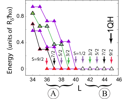
Figure 1: CI-calculated, relative-ground-state LLL energy spectra for $N=9$ fermions associated with the contact-interaction term only; see third term of $H_{\rm LLL}$ in Eq. (1). Spectra in a given spin sector $S=1/2,3/2,5/2,7/2$ and $S=9/2$ are expilcitly denoted. The spectra were calculated for $S_{z}=1/2$; however, they are independent of the precise value of $S_{z}$. The 0IE states of family $A$ are colored in red; those of family $B$ are colored in white. The first quasi-hole state is also explicitly denoted. $L$ is the total angular momentum.

In CI calculations and for a given number $N$ of spinful LLL fermions, the 0IE states emerge in each spin sector $(S,S_{z})$; see Fig. 1 for the case of $N=9$ LLL fermions interacting with a $\sum_{i<j}\delta(z_{i}-z_{j})$ two-body potential, where $z_{i}=x_{i}+iy_{i}$ (with $i=1,2,\ldots,N$). Interest in such 0IE states arises from: (i) They can be prepared experimentally palm20 . (For bosons, the experimental expectations for 0IE states include fittingly the $\nu=1/2$ bosonic Laughlin state popp04 ; hazz08 ; dali11 .) (ii) They represent microscopic states that describe quantum LLL skyrmions brey96 ; note1 . (iii) The Laughlin states are 0IE eigenstates associated with short-range pseudopotential-type Hamiltonians hald83 ; simochap . (iv) For fully polarized fermions, 0IE states have been associated with the gapless edge excitations of the Laughlin droplet wen92 in extended semiconductor samples.

The many-body Hamiltonian describing ultracold neutral atoms in a rapidly rotating trap popp04 ; yann06 ; yann07.2 ; coop08 ; hazz08 ; palm20 is given by

$$\frac{H_{\rm LLL}}{\hbar\omega}=N+(1-\frac{\Omega}{\omega})L+2\pi R_{\delta}\sum_{i<j}^{N}\delta(z_{i}-z_{j}),$$ (1)

where $\omega$ and $\Omega$ are, respectively, the parabolic trapping and rotational frequencies of the trap, and $L$ denotes the total angular momentum, $L=\sum_{i=1}^{N}\ l_{i}$, normal to the rotating-trap plane; the energies are in units of $\hbar\omega$ and the lengths in units of the oscillator length $\Lambda=\sqrt{\hbar/(M\omega)}$, with $M$ being the fermion mass. The first and second terms express the LLL kinetic energy, $H_{K}$, and the third term represents the contact interaction, $H_{\rm int}$.

Our methodology integrating both numerical (e.g., fortran) and symbolic (algebraic, e.g., MATHEMATICA math ) languages consists of two steps: (1) numerical diagonalization of the Hamiltonian matrix problem employing the ARPACK solver arpack ; arno51 of large-scale sparse eigenvalue problems, followed by step (2) where the numerically exact CI wave functions

$$\Phi_{\rm CI}(z_{1}\sigma_{1},\ldots,z_{N}\sigma_{N})=\sum_{I}c_{\rm CI}(I)\Psi_{I}(z_{1}\sigma_{1},\ldots,z_{N}\sigma_{N}),$$ (2)

are analyzed and processed using symbolic scripts targeting extraction of the corresponding exact analytical wave functions.

The basis Slater determinants that span the Hilbert space are

$$\Psi_{I}={\rm Det}[\varphi_{j_{r}}(z_{s})\sigma_{j_{r}}(s)]/\sqrt{N!},$$ (3)

where $r,s=1,\ldots,N$, the LLL single-particle orbitals are

$$\varphi_{j}(z)=z^{l_{j}}e^{-zz^{*}/2}/\sqrt{\pi l_{j}!},$$ (4)

and $\sigma$ signifies an up ($\alpha$) or a down ($\beta$) spin. The master index $I$ counts the number of ordered arrangements (lists) $\{j_{1},j_{2},\ldots,j_{N}\}$ under the restriction that $1\leq j_{1}<j_{2}<\ldots<j_{N}\leq K$; $K\in\mathbb{N}$ is chosen large enough to provide numerical convergence. Below, explicit mention of the Gaussian factor is omitted.

Step (2) starts with the rewriting of the CI wave function $\Phi_{\rm CI}$ in Eq. (2) as

$$\Phi_{\rm alg}(z_{1}\sigma_{1},\ldots,z_{N}\sigma_{N})=\sum_{I}c_{\rm alg}(I)\Psi_{I}(z_{1}\sigma_{1},\ldots,z_{N}\sigma_{N}),$$ (5)

where the replacement of the subscript “CI” by “alg” corresponds to the fact that, using the symbolic language code, one obtains an equivalent multivariate homogeneous polynomial $\Phi_{\rm alg}$ with algebraic coefficients $c_{\rm alg}$; see the transcription of coefficients for $N=4$ and $N=9$ in Tables STI and STII in the SM supp .

Validation of our closed-form analytic wave functions (see below) is achieved via direct comparison of the numerical CI coefficients, $c_{\rm CI}$, with those in $\Phi_{\rm alg}$ [Eq. (5)], thus circumventing uncertainties, associated with the common use of wave function overlap laug83 ; simochap ; jainbook ; palm20 ; yoso98 , due to the van Vleck-Anderson orthogonality catastrophe vlec36 ; ande67 ; kohn99 ; deml12 ; guzi14 ; ares18 ; gu19 .

Invariably, the symbolic code is able to simplify the derived multivariate polynomial in Eq. (5) to the compact form of a product of a Vandermonde determinant (VDdet), $\prod_{i<j}^{N}(z_{i}-z_{j})$, involving the space coordinates only, with a symmetric polynomial (under two-particle exchange) with mixed space and spin coordinates [see Eq. (6) below]. The factoring out of the VDdet reflects the fact that $\Phi_{\rm alg}$ represents a 0IE LLL state.

Using symbolic scripts, we verify further that the fully-algebraic $\Phi_{\rm alg}$ [Eq. (6)] is indeed an eigenstate of the total spin, obeying the Fock condition fock40 . The final closed form expressions [see Eq. (8) below] are derived for $N\leq 9$, but they are valid for any $N$, thus circumventing the CI numerical diagonalization of large matrices, which is not feasible for $N\geq\sim 10$.

For the CI diagonalization, a small perturbing term $V_{P}$ (e.g., a small trap deformation yann20 , or a small hard-wall boundary maca17 ) needs to be added to the LLL Hamiltonian in Eq. (1). This has a negligible influence on the numerical eigenvalues, but it is instrumental in lifting the degeneracies among the 0IE states, and thus produce CI states whose total spin $S$ is a good quantum number.

III Targeted total spins and angular momenta

For each size $N$, we provide analytic expressions for the maximum-spin ($S=S_{z}$) 0IE ground states with angular momenta $L=L_{0}+\Delta L$ [with $L_{0}=N(N-1)/2$] from $\Delta L=0$ (maximum density droplet) to $\Delta L=N$ (first quasihole, 1QH); they form two families $A$ and $B$ (see Fig. 1 for an illustration).

Using $k$ to denote the number of spin-up fermions and $p$ that of spin-down fermions, and focusing on the case with $k\geq p$ (or equivalently $p\leq N/2$), the states in both families are associated with the same set of total spins specified as $S=S_{z}=(k-p)/2=N/2-p$. Furthermore, given a pair $(k,p)$:

(A) The states in family $A$ have $\Delta L=p$, with $\Delta L$ varying from 0 to $N/2$ for even $N$, and from 0 to $(N-1)/2$ for odd $N$.

(B) The states in family $B$ have $\Delta L=k$, with $\Delta L$ varying from $N/2$ to $N$ for even $N$, and from $(N+1)/2$ to $N$ for odd $N$.

The states in family $A$ are unique ground states, whereas those in family $B$ are part of degenerate manifolds. (This degeneracy is lifted as described above.)

IV The exact 0IE LLL wave functions

IV.0.1 Mathematical preliminary

The quantity $k$-subset($list$) is a subset containing exactly $k$ elements out of the set of $n$ elements (named $list$). The number of $k$-subsets on $n$ elements is given by $\left(\frac{n}{k}\right)=\frac{n!}{k!(n-k)!}$. The set represented by $list$ is taken to be a list of cardinally ordered positive integers. For example, there are 6 2-subsets when $list$={1,2,3,4}, namely {1,2}, {1,3}, {1,4}, {2,3}, {2,4}, and {3,4}.

IV.0.2 General form of the 0IE LLL wave functions

The compact algebraic expression has the general form

$$\Phi_{\rm alg}\big{(}z_{1}\chi(1), \ldots,z_{N}\chi(N)\big{)}\propto\Phi_{V}(l_{1},\ldots,l_{N};z_{1},\ldots,z_{N})$$

$$\times\Phi_{\rm sym}\big{(}z_{1}\chi(1),\ldots,z_{N}\chi(N)\big{)},$$ (6)

where $\chi(i)$ denotes an up spin, $\alpha$, or down spin, $\beta$, and $i=1,\ldots,N$.

$\Phi_{V}$ is a Vandermonde determinant,

$$\Phi_{V}([l];[z])={\rm Det}[z_{i}^{l_{j}}]=\prod_{i<j}^{N}(z_{i}-z_{j}),$$ (7)

where $l_{j}=(j-1)$ and $i,j=1,2,\ldots,N$. The product of Jastrow factors above reflects the fact that the wave function in Eq. (6) is a 0IE eigenstate of the contact-interaction term, $H_{\rm int}$, in Eq. (1).

Due to the fermionic symmetry of the $\Phi_{\rm alg}$, $\Phi_{\rm sym}$ has to be symmetric under the exchange of any pair of indices $i$ and $j$. Furthermore, $\Phi_{\rm sym}$ can be written as

$$\Phi_{\rm sym}\big{(}z_{1}\chi(1),\ldots,z_{N}\chi(N)\big{)}=\sum_{m=1}^{K}{\cal P}_{m}^{o}[z]{\cal Z}_{m},$$ (8)

where ${\cal P}_{m}^{o}$ (defined below) are homogeneous multivariate polynomials of order $o=p$ (family $A$) or $o=k$ (family $B$), and

$${\cal Z}_{m}=\alpha(i_{1})\alpha(i_{2})\ldots\alpha(i_{k})\beta(j_{k+1})\ldots\beta(j_{N}),$$ (9)

is one of the $K=N!/(k!p!)$ distinct spin primitives having $k\leq N$ up and $p=N-k\leq k$ down spins. The set of indices $\{i_{1},\ldots,i_{k}\}$ is the $m$th element ($m=1,2,\ldots,K$) of the $k$-subsets of the cardinal list (top-level $list$, see below) specified as $list$={1,2,…,$N$}. The set of indices $\{j_{k+1},\ldots,j_{N}\}$ is complementary to the $\{i_{1},\ldots,i_{k}\}$ set.

The $\Phi_{V}$ [Eq. (7)] corresponds to a filling factor $\nu=1$, whereas the filling fraction corresponding to Eq. (6) [with $\Phi_{\rm sym}$ given in Eq. (8) through polynomials of order $o$] is near $\nu=1$. These fractions are indeed the ones most likely to be accessed first in upcoming experiments palm20 .

IV.0.3 Algebraic expressions for the polynomials ${\cal P}_{m}^{o}([z])$

For each $S=S_{z}=(k-p)/2$, except when $k=p$ which has a single state, there exists a pair of targeted LLL states, with one state of the pair belonging to family $A$ and the other to family $B$ (see Fig. 1 for an example).

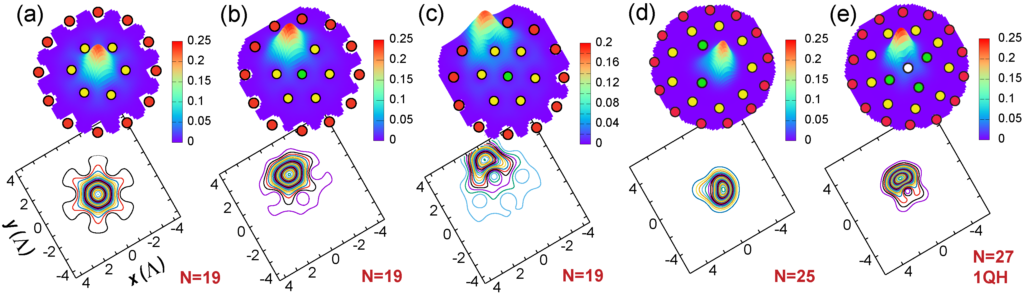
Figure 2: $N$th-order spin-unresolved correlations for $N$ LLL fermions. (a,b,c) $N=19$ with $L=180$, and $S=S_{z}=1/2$. (d) $N=25$ with $L=301$, and $S=S_{z}=23/2$. (e) $N=27$ with $L=378$, and $S=S_{z}=27/2$ (1QH state). Fixed fermions are marked by red dots for the outer ring, yellow dots for the middle ring, and green dots for the inner ring. The white dot for the 1QH state denotes the additional zero at the origin. Vertical axes: arbitrary units. See text for details. In the LLL, momentum correlations coincide with the spatial ones yann20 .

Family A: First, the following square matrices of rank $p$ (the number of spin-down fermions) need to be considered:

$${\rm M}_{q,m}=\left[\begin{array}[]{ccc}z_{i_{1}}-z_{j_{k+1}}&\dots&z_{i_{1}}-z_{j_{N}}\\ \vdots&\ddots&\vdots\\ z_{i_{p}}-z_{j_{k+1}}&\dots&z_{i_{p}}-z_{j_{N}}\\ \end{array}\right],$$ (13)

where the dummy indices $i_{1},\ldots,i_{p}$ here are associated with spin-up fermions, and the set $\{i_{1},\ldots,i_{p}\}$ denotes the $q$th subset among the $p$-subsets on a second-level $list$-2, with $list$-2 being the $m$th element among the $k$-subsets on the $\{1,2,\ldots,N\}$ top-level $list$. The number of $p$-subsets of any second-level $list$-2 is $K_{2}=k!/(p!(k-p)!)$, and thus the $q$ subscript runs from 1 to $K_{2}$. The set of indices $\{j_{k+1},\ldots,j_{N}\}$ is complementary to the $\{i_{1},\ldots,i_{k}\}$ set, and thus it remains constant for a given $m$ index in the matrices defined in Eq. (13). (Recall that $k$ is the total number of spin-up fermions, and that $\{i_{1},\ldots,i_{k}\}$ is also referred to as a second-level list.)

The expression for the polynomial is given by

$${\cal P}_{m}^{p}([z])=\sum_{q=1}^{K_{2}}{\rm Perm}[{\rm M}_{q,m}],$$ (14)

where the symbol ”Perm” denotes a Permanent.

The analytic expressions of the states with $S_{z}<S$, in a given spin multiplicity $2S+1$, are obtained by repeated application of the spin lowering operator.

Example. We consider the state associated with $N=5$, $S=S_{z}=1/2$, and $L=12$. Note that $L_{0}=N(N-1)/2=10$ in the corresponding fully polarized case. There are $K=5!/(3!2!)=10$ spin primitives ${\cal Z}_{m}$, with $m=1,2,\ldots,10$; they correspond to the ten 3-subsets on the top-level $list$=$\{1,2,3,4,5\}$, i.e., $\{1,2,3\}$ ($m=1$), $\{1,2,4\}$ ($m=2$), $\{1,2,5\}$ ($m=3$), $\{1,3,4\}$ ($m=4$), $\{1,3,5\}$ ($m=5$), $\{1,4,5\}$ ($m=6$), $\{2,3,4\}$ ($m=7$), $\{2,3,5\}$ ($m=8$), $\{2,4,5\}$ ($m=9$), $\{3,4,5\}$ ($m=10$).

Here $k=3$, $p=2$, and there are $K_{2}=3$ 2-subsets for each ($m$th) 3-subset listed above. $K_{2}=3$ is also the number of permanents entering in expression (14), i.e., $q=1,\dots,3$. Choosing $m=10$ as an example, the three 2-subsets are $\{3,4\}$, $\{3,5\}$, and $\{4,5\}$, and the three associated matrices ${\rm M}_{q,10}$ are given by:

$${\rm M}_{q,10}=\left[\begin{array}[]{ccc}\eta(q,1)-z_{1}&\eta(q,1)-z_{2}\\ \eta(q,2)-z_{1}&\eta(q,2)-z_{2}\\ \end{array}\right],$$ (17)

with with $q=1,2,3$; $\eta(1,1)=z_{3}$, $\eta(1,2)=z_{4}$, $\eta(2,1)=z_{3}$, $\eta(2,2)=z_{5}$, and $\eta(3,1)=z_{4}$, $\eta(3,2)=z_{5}$.

An additional example is presented in the SM supp .

Family B: Similarly, we found that the symmetric polynomials ${\cal P}_{m}^{k}([z])$ related to the ground states of family $B$ consist always [for any $m$ in the summation of Eq. (8)] of a single permanent associated with a matrix of rank $k$ (the number of spin-up fermions). Namely

$${\cal P}_{m}^{k}([z])={\rm Perm}[{\rm M}_{m}^{B}],$$ (18)

with

$${\rm M}_{m}^{B}=$$

$$\left[\begin{array}[]{cccccc}z_{i_{1}}-z_{j_{k+1}}&\dots&z_{i_{1}}-z_{j_{N}}&z_{i_{1}}-z_{j_{N+1}}&\ldots&z_{i_{1}}-z_{j_{2k}}\\ \vdots&\ddots&\vdots&\vdots&\ddots&\vdots\\ z_{i_{k}}-z_{j_{k+1}}&\dots&z_{i_{k}}-z_{j_{N}}&z_{i_{k}}-z_{j_{N+1}}&\ldots&z_{i_{k}}-z_{j_{2k}}\\ \end{array}\right].$$ (22)

Above, the set of indices $\{i_{1},\ldots,i_{k}\}$ is the $m$th element of the $k$-subsets associated with the spin-up fermions [see Eq. (9)]. Because $k>p$, the complimentary set of the $p$ spin-down indices $\{j_{k+1},\ldots,j_{N}\}$ has been expanded to contain exactly $k$ elements, through the introduction of virtual fermion coordinates such that $z_{j_{s}}=0$ for all $s>N$; see specific matrices ${\rm M}_{m}^{B}$, as well as a comparison with the wave functions in Ref. brey96 , in the Appendix and the SM supp .

Note that the first quasi-hole state (1QH) laug83 ; maca17 coincides with the analytic expression associated with family $B$ above for $L=L_{0}+N$.

V Higher-order correlations

We used the analytic wave functions above to calculate spin-unresolved higher-oder correlations for $N=19$, 25, and 27 fermions; see Fig. 2 (for completeness, see Fig.  SF3 for $N=9$ in the SM supp ). The $n$-body correlations for spinful fermions were defined in detail in Sec. II C of Ref. yann20 . For the $N$-body $\Phi_{\rm alg}$ [Eq. (6)], the spatial $n$-body correlation is given in a compact form by

$${\cal G}^{n} (N)=(1-\delta_{n,N})\int|\Phi_{\rm alg}\big{(}z_{1}\chi(1),\ldots,z_{N}\chi(N)\big{)}|^{2}\times$$

$$dz_{n+1}d\chi(n+1)\ldots dz_{N}d\chi(N)+\delta_{n,N}|\Phi_{\rm alg}|^{2},$$ (23)

with $n=2,\dots,N$. ${\cal G}^{n}(N)$ gives the conditional probablility to find particles $n,\ldots,N$ anywhere, for prespecified (fixed) locations of particles $1,\ldots,n-1$ with predetermined (resolved) or unspecified (unresolved) spins.

For $N=19$, Figs. 2(a,b,c) display structured $N$th-order correlations for the spin state with $S=S_{z}=1/2$ and total angular momentum $L=180$. Extending Ref. yann20 , we found similar crystalline structures also in the $N$th-order correlations of the associated fully polarized, single VDdet state with $S=19/2$, $S_{z}=19/2$, and $L_{0}=171$ (Pauli-exclusion-only case, experimentally investigated holt20 ). Fig. 2(d) displays the structured $N$th-order correlation for $N=25$ with $L=301$ and $S=S_{z}=23/2$, whereas Fig. 2(e) presents the structured $N$th-order correlations for the 1QH for $N=27$ (with $L=378$ and $S=S_{z}=27/2$). The implied intrinsic geometric structure (UCWM) in Fig. 2 is a polygonal triple ring $(n_{1},n_{2},n_{3})$ of localized fermions (with $n_{1}+n_{2}+n_{3}=N$); specifically (1,6,12), (3,9,13), and (4,9,14) for Figs. 2(a,b,c), Fig. 2(d), and Fig. 2(e), respectively. We note that in the LLL neighbohood of $\nu=1$ (expected in experiments with trapped ultracold fermions palm20 ), the intrinsic ring geometry can be probed only with higher-order correlations. Indeed in this case, the second-order correlations are structureless; see the findings for $N=4$ [(0,4) single ring] and $N=6$ [(1,5) double ring] in Ref. yann20 .

VI Conclusion

A novel approach for deriving exact closed-form analytic expressions for the wave functions (beyond the Jastrow-factors paradigm) of an assembly of 2D contact-interacting spinful LLL fermions (for any $N$) was introduced and validated. Such expressions require as input only the three parameters $N$ (number of particles), $L$ (total angular momentum), and $S$ (total spin). Examples were presented for two families of zero-interaction-energy states, from the maximum density droplet to the first quasihole in the neighborhood of $\nu=1$. Ensuing theoretical predictions for higher-order momentum correlations for $N=19$, 25, and 27, revealing intrinsic polygonal, multi-ring crystalline configurations, could be tested with ultracold-atom experiments in rotating traps simulating spinful quantum Hall physics, including LLL skyrmions. The present approach can be extended to the neighborhood of any $\nu=1/m$ that starts with a Laughlin wave function.

VII Acknowledgments

This work has been supported by a grant from the Air Force Office of Scientific Research (AFSOR) under Award No. FA9550-21-1-0198. Calculations were carried out at the GATECH Center for Computational Materials Science.

*

Appendix A Comparison with the symmetric polynomials for quantum skyrmions in Ref. brey96

We compare here with the symmetric polynomials for the seed skyrmions specified in Eq. (6) of Ref. brey96 or Eq. (2) in Ref. jain96 .

Omitting the trivial Gaussian functions, these polynomials are given by the single formula

$$\Phi^{\rm sk,MFB}_{p}=\sum_{m=1}^{K}z_{i_{1}}z_{i_{2}}...z_{i_{k}}{\cal Z}_{m},$$ (24)

where ${\cal Z}_{m}$ are the spin primitives defined in Eq. (9), and the superscript MFB stands for MacDonald-Fertig-Brey. The index $m$ runs also over the $k$-subsets $\{i_{1},\ldots,i_{k}\}$ of the $list=\{1,2,3,\ldots,N\}$, $k=N\!\uparrow$ being the number of spin-up fermions, with $p=N-k=N\!\downarrow$ being that of the spin-down fermions. The number of $k$-subsets is $K=N!/(k!p!)$. As is the case in Ref. brey96 , one can take the index $m$ as running over the $p$-subsets associated with the spin-down fermions, because there is a one-to-one correspondence to the $k$-subsets of the spin-up fermions. Note that Ref. brey96 (Ref. jain96 ) uses the capital letter $K$ ($R$) in place of our $p$.

We consider the case $N=5$, $k=4$, $p=1$, $S=S_{z}=3/2$, and $\Delta L=4$, belonging to family $B$ in our exposition.

According to Eq. (24), the corresponding MFB symmetric polynomial is

$$\begin{split}\Phi^{\rm sk,MFB}_{p=1}=&z_{1}z_{2}z_{3}z_{4}{\cal Z}_{1}+z_{1}z_{2}z_{3}z_{5}{\cal Z}_{2}+z_{1}z_{2}z_{4}z_{5}{\cal Z}_{3}+\\ &z_{1}z_{3}z_{4}z_{5}{\cal Z}_{4}+z_{2}z_{3}z_{4}z_{5}{\cal Z}_{5}.\end{split}$$ (25)

The corresponding exact symmetric polynomial derived in this paper is given by Eqs. (8) and (18), namely

$$\Phi^{\rm exact}_{\rm sym}(N=5,N\!\uparrow=4,\Delta L=4)=\sum_{m=1}^{5}{\cal P}^{4}_{m}[z]{\cal Z}_{m},$$ (26)

Expanding the permanents, one obtains for the space-only polynomials ${\cal P}^{4}_{m}[z]$ above (with $m=1,\ldots,5$, in front of the ${\cal Z}_{m}$ spin primitives):

$$\begin{split}{\cal P}^{4}_{m}[z]=&c_{1}z_{1}z_{2}z_{3}z_{4}+c_{2}z_{1}z_{2}z_{3}z_{5}+c_{3}z_{1}z_{2}z_{4}z_{5}+\\ &c_{4}z_{1}z_{3}z_{4}z_{5}+c_{5}z_{2}z_{3}z_{4}z_{5},\end{split}$$ (27)

with $c_{i}=4$ when $i=m$ and $c_{i}=-1$ otherwise.

The polynomial in Eq. (26) is clearly different from the MFB one [Eq. (25)]. We verified that the wave functions derived here are eigenfunctions of the square, $\hat{S}^{2}$, of the total-spin operator [with eigenvalue 15/4 and $S=3/2$ for the case in this Appendix], whereas the MFB ones are not (see also Ref. abol97 ); for details see Ref. supp .

Contents:
     
1) Contrast with the symmetric polynomials for skyrmions in earlier literature, p. 9
     
2) Additional specific examples of the compact analytic wave functions derived in the main text, p. 10
    
3) Tables illustrating, for $N=4$ and $N=9$, the correspondence between numerical CI and algebraic coefficients in the determinantal expansions of $\Phi_{\rm CI}$ and $\Phi_{\rm alg}$, p. 11
       
4) Figure displaying additional higher-order correlations for $N=9$ LLL fermions, p.12        
       
       
      
      
^†Constantine.Yannouleas@physics.gatech.edu
^∗Uzi.Landman@physics.gatech.edu

Comparison with symmetric polynomials for skyrmions in previous literature

We compare here with the symmetric polynomials for the seed skyrmions specified in Eq. (6) of (R1) A. H. MacDonald, H. A. Fertig, and Luis Brey, Skyrmions without Sigma Models in Quantum Hall Ferromagnets, Phys. Rev. Lett. 76, 2153 (1996) (https://doi.org/10.1103/PhysRevLett.76.2153); see also Eq. (2) in (R2) R.K. Kamilla, X.G. Wu, and J.K. Jain, Skyrmions in the fractional quantum Hall effect, Solid State Commun. 99, 289 (1996) (https://doi.org/10.1016/0038-1098(96)00126-3).

Omitting the trivial Gaussian functions, these polynomials are given by the single formula

$$\Phi^{\rm sk,MFB}_{p}=\sum_{m=1}^{K}z_{i_{1}}z_{i_{2}}...z_{i_{k}}{\cal Z}_{m},$$ (S28)

where ${\cal Z}_{m}$ are the spin primitives defined in Eq. (9) of the main text, i.e.,

$${\cal Z}_{m}=\alpha(i_{1})\alpha(i_{2})\ldots\alpha(i_{k})\beta(j_{k+1})\ldots\beta(j_{N}).$$ (S29)

The index $m$ runs also over the $k$-subsets $\{i_{1},\ldots,i_{k}\}$ of the $list=\{1,2,3,\ldots,N\}$, $k=N\!\uparrow$ being the number of spin-up fermions, with $p=N-k=N\!\downarrow$ being that of the spin-down fermions. The number of $k$-subsets is $K=N!/(k!p!)$. As is the case in Ref. R1, one can take the index $m$ as running over the $p$-subsets associated with the spin-down fermions, because there is a one-to-one correspondence to the $k$-subsets of the spin-up fermions. Note that Ref. R1 (Ref. R2) uses the capital letter $K$ ($R$) in place of our $p$.

We present here a comparison for the case $N=5$, $k=4$, $p=1$, $S=S_{z}=3/2$, and $\Delta L=4$, a state belonging to family B in our exposition.

According to Eq. (S28), the corresponding MacDonald-Fertig-Brey (MFB) symmetric polynomial is

$$\Phi^{\rm sk,MFB}_{p=1}=z_{1}z_{2}z_{3}z_{4}{\cal Z}_{1}+z_{1}z_{2}z_{3}z_{5}{\cal Z}_{2}+z_{1}z_{2}z_{4}z_{5}{\cal Z}_{3}+z_{1}z_{3}z_{4}z_{5}{\cal Z}_{4}+z_{2}z_{3}z_{4}z_{5}{\cal Z}_{5}.$$ (S30)

The corresponding polynomial derived in this paper is given by Eqs. (8) and (13) in the main text. Expanding the permanent, one obtains for the polynomial with $k=4$ and $m=1$ (in front of the ${\cal Z}_{1}$ spin primitive):

$${\cal P}^{4}_{1}[z]=4z_{1}z_{2}z_{3}z_{4}-z_{1}z_{2}z_{3}z_{5}-z_{1}z_{2}z_{4}z_{5}-z_{1}z_{3}z_{4}z_{5}-z_{2}z_{3}z_{4}z_{5}.$$ (S31)

For the ${\cal P}^{4}_{2}$ polynomial in front of ${\cal Z}_{2}$, one obtains similarly:

$${\cal P}^{4}_{2}[z]=-z_{1}z_{2}z_{3}z_{4}+4z_{1}z_{2}z_{3}z_{5}-z_{1}z_{2}z_{4}z_{5}-z_{1}z_{3}z_{4}z_{5}-z_{2}z_{3}z_{4}z_{5}.$$ (S32)

In general, one has

$$\Phi^{\rm exact}_{\rm sym}(N=5,N\!\uparrow=4,\Delta L=4)=\sum_{m=1}^{5}{\cal P}^{4}_{m}[z]{\cal Z}_{m},$$ (S33)

with

$${\cal P}^{4}_{m}[z]=c_{1}z_{1}z_{2}z_{3}z_{4}+c_{2}z_{1}z_{2}z_{3}z_{5}+c_{3}z_{1}z_{2}z_{4}z_{5}+c_{4}z_{1}z_{3}z_{4}z_{5}+c_{5}z_{2}z_{3}z_{4}z_{5},$$ (S34)

and $c_{i}=4$ when $i=m$ and $c_{i}=-1$ otherwise.

We note that the expressions associated with the ${\cal Z}_{i}$, $i=1,\ldots,5$ in the MFB polynomial consist only of a single term with a numerical factor +1 in front. This contrasts with our expressions in Eqs. (S31), (S32), and (S34) which have five terms each with factors of +4 and -1 in front of them.

For $p$ (spin-down fermions) $>$ $k$ (spin-up fermions), the MFB expression in Eq. (S28) is associated with a negative total-spin projection $S_{z}=(k-p)/2<0$. In this case, the indices for the corresponding wave function in this paper are found by reversing all $N$ spins, i.e., by considering the case with $p\rightarrow k$, $k\rightarrow p$, and $S_{z}=|(k-p)/2|$.

Using our algebraic scripts, we readily verified that the wave functions derived in this work are indeed eigenfunctions of the total-spin square operator [with eigenvalue 15/4 and $S=3/2$ for the case in this section], whereas the MFB ones are not (as indeed has been discussed by M. Abolfath et al., Phys. Rev. B 56, 6795 (1997) (https://doi.org/10.1103/PhysRevB.56.6795).

In particular, applying the spin-square, $\hat{S}^{2}$, operator, one gets

$$\big{(}\hat{S}^{2}-\frac{15}{4}\big{)}\Phi^{\rm exact}_{\rm sym}(N=5,N\!\uparrow=4,\Delta L=4)=0.$$ (S35)

On the contrary, for the MFB wave function, one gets

$$\big{(}\hat{S}^{2}-\frac{15}{4}\big{)}\Phi^{\rm sk,MFB}_{p=1}=(z_{1}z_{2}z_{3}z_{4}+z_{1}z_{2}z_{3}z_{5}+z_{1}z_{2}z_{4}z_{5}+z_{1}z_{3}z_{4}z_{5}+z_{2}z_{3}z_{4}z_{5})\sum_{m=1}^{5}{\cal Z}_{m}.$$ (S36)

=====================================================

Additional examples for the wave functions in families $A$ and $B$

Family $A$. As another example from family $A$, we consider the spin singlet state associated with $N=4$, $S=0$, $S_{z}=0$, and $L=8$. Note that $L_{0}=N(N-1)/2=6$ in the corresponding fully spin-polarized case. There are $K=4!/(2!2!)=6$ spin primitives ${\cal Z}_{m}$, with $m=1,2,\ldots,6$; they correspond to the six 2-subsets on the top-level $list=\{1,2,3,4\}$, i.e., $\{1,2\}$ ($m=1$), $\{1,3\}$ ($m=2$), $\{1,4\}$ ($m=3$), $\{2,3\}$ ($m=4$), $\{2,4\}$ ($m=5$), $\{3,4\}$ ($m=6$).

Because $k=2$ and $p=2$, there is only one ($K_{2}=1$) 2-subset for each ($m$th) 2-subset listed above. $K_{2}=1$ is also the number of permanents entering in expression (11) of the main text, i.e., the index $q$ takes only the value of one. Choosing $m=2$ as an example, the single matrix ${\rm M}_{1,2}$ is:

$${\rm M}_{1,2}=\left[\begin{array}[]{ccc}z_{1}-z_{2}&z_{1}-z_{4}\\ z_{3}-z_{2}&z_{3}-z_{4}\\ \end{array}\right].$$ (S39)

Family $B$. First example. As a first example from family $B$, we consider the spin $S=S_{z}=3/2$ state associated with $N=9$ and $L=42$. Note that $L_{0}=N(N-1)/2=36$. There are $k=6$ up spins, $p=3$ down spins, and $K=9!/(6!3!)=84$ spin primitives ${\cal Z}_{m}$, with $m=1,2,\ldots,84$.

Focusing on the $m=1$ spin primitive, we have a subset of indices $\{i_{1},i_{2},\ldots,i_{6}\}$ for the spin up fermions and a subset of indices $\{j_{7},j_{8},j_{9}\}$ for the spin down fermions. The subset of the spin down indices needs to be augmented by introducing three additional indices $\{j_{10},j_{11},j_{12}\}$, which specify virtual fermions with $z_{j_{10}}=z_{j_{11}}=z_{j_{12}}=0$. Then the corresponding matrix ${\rm M}_{1}^{B}$ [see Eq. (14) in the main text] is given by

$${\rm M}_{1}^{B}=\left[\begin{array}[]{cccccc}z_{i_{1}}-z_{j_{7}}&z_{i_{1}}-z_{j_{8}}&z_{i_{1}}-z_{j_{9}}&z_{i_{1}}&z_{i_{1}}&z_{i_{1}}\\ z_{i_{2}}-z_{j_{7}}&z_{i_{2}}-z_{j_{8}}&z_{i_{2}}-z_{j_{9}}&z_{i_{2}}&z_{i_{2}}&z_{i_{2}}\\ z_{i_{3}}-z_{j_{7}}&z_{i_{3}}-z_{j_{8}}&z_{i_{3}}-z_{j_{9}}&z_{i_{3}}&z_{i_{3}}&z_{i_{3}}\\ z_{i_{4}}-z_{j_{7}}&z_{i_{4}}-z_{j_{8}}&z_{i_{4}}-z_{j_{9}}&z_{i_{4}}&z_{i_{4}}&z_{i_{4}}\\ z_{i_{5}}-z_{j_{7}}&z_{i_{5}}-z_{j_{8}}&z_{i_{5}}-z_{j_{9}}&z_{i_{5}}&z_{i_{5}}&z_{i_{5}}\\ z_{i_{6}}-z_{j_{7}}&z_{i_{6}}-z_{j_{8}}&z_{i_{6}}-z_{j_{9}}&z_{i_{6}}&z_{i_{6}}&z_{i_{6}}\\ \end{array}\right].$$ (S46)

Family $B$. Second example. As a second example from family $B$, we consider the 1QH state for $N=9$. In this case, $S=S_{z}=9/2$ and $L=45$. Note that $L_{0}=N(N-1)/2=36$. There are $k=9$ up spins, $p=0$ down spins, and $K=9!/(9!0!)=1$ spin primitive ${\cal Z}_{1}$.

For this single spin primitive, we have a subset of indices $\{i_{1},i_{2},\ldots,i_{9}\}$ for the spin up fermions and an empty subset of indices for the spin down fermions. The subset of the spin down indices needs to be augmented by introducing nine additional indices $\{j_{1},j_{2},\ldots,j_{9}\}$, which specify virtual fermions with $z_{j_{1}}=z_{j_{2}}=\ldots=z_{j_{9}}=0$. Then the corresponding matrix ${\rm M}_{1}^{B}$ [see Eq. (14) in the main text] is given by

$${\rm M}_{1}^{B}=\left[\begin{array}[]{ccccccccc}z_{i_{1}}&z_{i_{1}}&z_{i_{1}}&z_{i_{1}}&z_{i_{1}}&z_{i_{1}}&z_{i_{1}}&z_{i_{1}}&z_{i_{1}}\\ z_{i_{2}}&z_{i_{2}}&z_{i_{2}}&z_{i_{2}}&z_{i_{2}}&z_{i_{2}}&z_{i_{2}}&z_{i_{2}}&z_{i_{2}}\\ z_{i_{3}}&z_{i_{3}}&z_{i_{3}}&z_{i_{3}}&z_{i_{3}}&z_{i_{3}}&z_{i_{3}}&z_{i_{3}}&z_{i_{3}}\\ z_{i_{4}}&z_{i_{4}}&z_{i_{4}}&z_{i_{4}}&z_{i_{4}}&z_{i_{4}}&z_{i_{4}}&z_{i_{4}}&z_{i_{4}}\\ z_{i_{5}}&z_{i_{5}}&z_{i_{5}}&z_{i_{5}}&z_{i_{5}}&z_{i_{5}}&z_{i_{5}}&z_{i_{5}}&z_{i_{5}}\\ z_{i_{6}}&z_{i_{6}}&z_{i_{6}}&z_{i_{6}}&z_{i_{6}}&z_{i_{6}}&z_{i_{6}}&z_{i_{6}}&z_{i_{6}}\\ z_{i_{7}}&z_{i_{7}}&z_{i_{7}}&z_{i_{7}}&z_{i_{7}}&z_{i_{7}}&z_{i_{7}}&z_{i_{7}}&z_{i_{7}}\\ z_{i_{8}}&z_{i_{8}}&z_{i_{8}}&z_{i_{8}}&z_{i_{8}}&z_{i_{8}}&z_{i_{8}}&z_{i_{8}}&z_{i_{8}}\\ z_{i_{9}}&z_{i_{9}}&z_{i_{9}}&z_{i_{9}}&z_{i_{9}}&z_{i_{9}}&z_{i_{9}}&z_{i_{9}}&z_{i_{9}}\\ \end{array}\right].$$ (S56)

When expanded, the associated permanent yields one term only, namely, $9!z_{i_{1}}z_{i_{2}}z_{i_{3}}z_{i_{4}}z_{i_{5}}z_{i_{6}}z_{i_{7}}z_{i_{8}}z_{i_{9}}$, and thus the 1QH state here agrees with the analytic form introduced by Laughlin; see https://doi.org/10.1103/PhysRevLett.50.1395.

==================================================

Table STI: The 15 dominant numerical CI coefficients, $c_{\rm CI}(J)$, in the CI expansion of the relative LLL ground state, and the corresponding extracted algebraic ones, $c_{\rm alg}(J)$, for $N=4$ fermions with total angular momentum $L=8$ (first 0IE state) in the ($S=S_{z}=0$) spin sector of singlet states. The spinful-fermions Slater determinants are specified through the set of single-particle angular momenta and spins, $(l_{1}\uparrow,l_{2}\uparrow,l_{3}\downarrow,l_{4}\downarrow)$. The converged CI expansion included a much larger set of basis Slater determinants, but naturally the dominant ones are only relevant, namely those with coefficients $|c_{\rm CI}(I)|>0.001$.

$J$	$c_{\rm CI}(J)$	$c_{\rm alg}(J)$	$(l_{1}\uparrow,l_{2}\uparrow,l_{3}\downarrow,l_{4}\downarrow)$	$\sum_{i=1}^{4}l_{i}$
1	-0.28005598	$\frac{2}{\sqrt{51}}$	(0,1,3,4)	8
2	0.34299719	$-\sqrt{\frac{2}{17}}$	(0,2,2,4)	8
3	-0.14002799	$\frac{1}{\sqrt{51}}$	(0,3,1,4)	8
4	-0.29704427	$\sqrt{\frac{3}{34}}$	(0,3,2,3)	8
5	0.14002799	$-\frac{1}{\sqrt{51}}$	(0,4,1,3)	8
6	-0.24253563	$\frac{1}{\sqrt{17}}$	(1,2,1,4)	8
7	-0.17149861	$\frac{1}{\sqrt{34}}$	(1,2,2,3)	8
8	0.14002799	$-\frac{1}{\sqrt{51}}$	(1,3,0,4)	8
9	0.42008405	$-\sqrt{\frac{3}{17}}$	(1,3,1,3)	8
10	-0.14002799	$\frac{1}{\sqrt{51}}$	(1,4,0,3)	8
11	-0.24253562	$\frac{1}{\sqrt{17}}$	(1,4,1,2)	8
12	-0.29704427	$\sqrt{\frac{3}{34}}$	(2,3,0,3)	8
13	-0.17149861	$\frac{1}{\sqrt{34}}$	(2,3,1,2)	8
14	0.34299718	$-\sqrt{\frac{2}{17}}$	(2,4,0,2)	8
15	-0.28005598	$\frac{2}{\sqrt{51}}$	(3,4,0,1)	8

Table STII: A sample of the 1551 dominant numerical CI coefficients, $c_{\rm CI}(J)$, in the CI expansion of the relative LLL ground state, and the corresponding extracted algebraic ones, $c_{\rm alg}(J)$, for $N=9$ fermions with total angular momentum $L=40$ (first 0IE state) in the ($S=S_{z}=1/2$) spin sector. The spinful-fermions Slater determinants are specified through the set of single-particle angular momenta and spins, $(l_{1}\uparrow,l_{2}\uparrow,l_{3}\uparrow,l_{4}\uparrow,l_{5}\uparrow,l_{6}\downarrow,l_{7}\downarrow,l_{8}\downarrow,l_{9}\downarrow)$. The converged CI expansion included a much larger set of basis Slater determinants, but naturally the dominant ones are only relevant, namely those with coefficients $|c_{\rm CI}(I)|>0.001$.

$J$	$c_{\rm CI}(J)$	$c_{\rm alg}(J)$	$(l_{1}\uparrow,l_{2}\uparrow,l_{3}\uparrow,l_{4}\uparrow,l_{5}\uparrow,l_{6}\downarrow,l_{7}\downarrow,l_{8}\downarrow,l_{9}\downarrow)$	$\sum_{i=1}^{9}l_{i}$
1	-0.10319005	$4\sqrt{\frac{5}{7513}}$	(0,1,2,3,4,6,7,8,9)	40
2	0.11303906	$-4\sqrt{\frac{6}{7513}}$	(0,1,2,3,5,5,7,8,9)	40
3	-0.02063800	$\frac{4}{\sqrt{37565}}$	(0,1,2,3,6,4,7,8,9)	40
4	-0.10465386	$\frac{24}{\sqrt{52591}}$	(0,1,2,3,6,5,6,8,9)	40
5	0.02063800	$-\frac{4}{\sqrt{37565}}$	(0,1,2,3,7,4,6,8,9)	40
6	0.09789477	$-6\sqrt{\frac{2}{7513}}$	(0,1,2,3,7,5,6,7,9)	40
$\vdots$	$\vdots$	$\vdots$	$\vdots$	$\vdots$
1546	0.00872117	$-\frac{2}{\sqrt{52591}}$	(4,5,6,7,9,0,1,3,5)	40
1547	0.00827362	$-3\sqrt{\frac{2}{262955}}$	(4,5,6,7,9,0,2,3,4)	40
1548	-0.02136239	$2\sqrt{\frac{6}{52591}}$	(4,5,6,8,9,0,1,2,5)	40
1549	-0.01103148	$4\sqrt{\frac{2}{262955}}$	(4,5,6,8,9,0,1,3,4)	40
1550	0.02527631	$-2\sqrt{\frac{6}{37565}}$	(4,5,7,8,9,0,1,2,4)	40
1551	-0.02063801	$\frac{4}{\sqrt{37565}}$	(4,6,7,8,9,0,1,2,3)	40

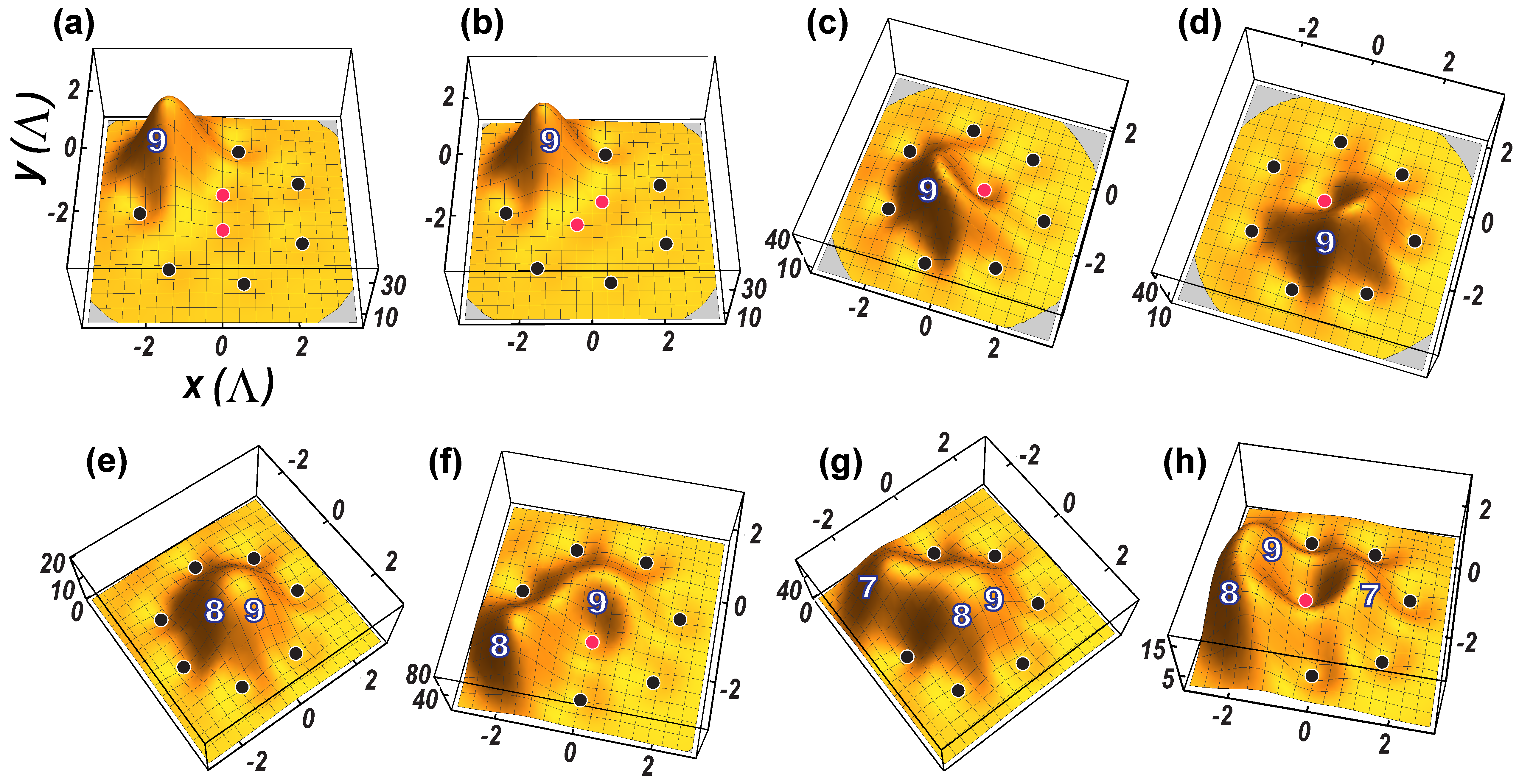
Figure SF3: Higher-order correlations for $N=9$ ultracold LLL fermions. (a-d) 9th-order correlations for the 0IE lowest-spin state ($S=1/2$, $S_{z}=1/2$) with total angular momentum $L=40$. Similar 9th-order correlations are found for the fully polarized state ($S=S_{z}=9/2$) with $L_{0}=36$. (e,f) 8th-order correlations for the fully polarized state ($S=9/2$, $S_{z}=9/2$) with $L_{0}=36$, whose space part is a pure Vandermonde determinant. (g,h) 7th-order correlations for the fully polarized state ($S=9/2$, $S_{z}=9/2$) with $L_{0}=36$. The implied intrinsic geometric structure (ultracold Wigner molecule) is a (2,7) double ring, with 2 fermions in the inner ring and 7 fermions in the outer ring. The fixed fermions are marked by solid dots (black for those in the outer ring and red for those in the inner ring). The white numbers denote the remaining, beyond the fixed ones, fermions. Vertical axes: arbitrary units.

References

- (1) M. Girardeau, Relationship between Systems of Impenetrable Bosons and Fermions in One Dimension, J. Math. Phys. 1, 516 (1960).
- (2) E.H. Lieb and W. Liniger, Exact Analysis of an Interacting Bose Gas. I. The General Solution and the Ground State, Phys. Rev. 130, 1605 (1963); M. Gaudin, Un système a une dimension de fermions en interaction, Phys. Lett. A 24 55 (1967); C.N. Yang, Some Exact Results for the Many-Body Problem in one Dimension with Repulsive Delta-Function Interaction, Phys. Rev. Lett. 19, 1312 (1967).
- (3) J.B. McGuire, Study of Exactly Soluble One-Dimensional -Body Problems, J. Math. Phys. 5, 622 (1964).
- (4) F. Calogero, Solution of the one-dimensional -body problem with quadratic and/or inversely quadratic pair potentials, J. Math. Phys. 12, 419 (1971); Erratum: ibid. 37, 3646 (1996).
- (5) B. Sutherland, Exact Results for a Quantum Many-Body Problem in One Dimension, Phys. Rev. A 4, 2019 (1971).
- (6) D.C. Mattis, The Many-Body Problem: An Encyclopedia of Exactly Solved Models in One Dimension (World Scientific, Singapore, 1993).
- (7) B. Sutherland, Beautiful Models: 70 Years of Exactly Solved Quantum Many-Body Problems (World Scientific, Singapore, 2004).
- (8) M.D. Girardeau, E.M. Wright, and J.M. Triscari, Ground-state properties of a one-dimensional system of hard-core bosons in a harmonic trap, Phys. Rev. A 63, 033601 (2001).
- (9) M.D. Girardeau and A. Minguzzi, Soluble Models of Strongly Interacting Ultracold Gas Mixtures in Tight Waveguides, Phys. Rev. Lett. 99, 230402 (2007).
- (10) M.D. Girardeau, Two super-Tonks-Girardeau states of a trapped one-dimensional spinor Fermi gas, Phys. Rev. A 82, 011607(R) (2010).
- (11) L. Guan, S. Chen, Y. Wang, and Z.-Q. Ma, Exact Solution for Infinitely Strongly Interacting Fermi Gases in Tight Waveguides, Phys. Rev. Lett. 102, 160402 (2009).
- (12) X. Cui and T-L Ho, Ground-state ferromagnetic transition in strongly repulsive one-dimensional Fermi gases, Phys. Rev. A 89, 023611 (2014).
- (13) F. Deuretzbacher, D. Becker, J. Bjerlin, S.M. Reimann, and L. Santos, Quantum magnetism without lattices in strongly interacting one-dimensional spinor gases, Phys. Rev. A 90, 013611 (2014).
- (14) A.G. Volosniev, D.V. Fedorov, A.S. Jensen, M. Valiente, and N.T. Zinner, Strongly interacting confined quantum systems in one dimension, Nat. Commun. 5, 5300 (2014).
- (15) J. Levinsen, P. Massignan, G.M. Bruun, and M.M. Parish, Strong-coupling ansatz for the one-dimensional Fermi gas in a harmonic potential, Science Advances 1, e1500197 (2015).
- (16) L. Yang and X. Cui, Effective spin-chain model for strongly interacting one-dimensional atomic gases with an arbitrary spin, Phys. Rev. A 93, 013617 (2016).
- (17) M. Beau, S.M. Pittman, G.E. Astrakharchik, and A. del Campo, Exactly Solvable System of One-Dimensional Trapped Bosons with Short- and Long-Range Interactions, Phys. Rev. Lett. 125, 220602 (2020).
- (18) M. Greiner, O. Mandel, T. Esslinger, Th.W. Hänsch, and I. Bloch, Quantum phase transition from a superfluid to a Mott insulator in a gas of ultracold atoms, Nature 415, 39 (2002).
- (19) F. Gerbier, A. Widera, S. Fölling, O. Mandel, T. Gericke, and I. Bloch, Phase Coherence of an Atomic Mott Insulator, Phys. Rev. Lett. 95, 050404 (2005).
- (20) F. Gerbier, A. Widera, S. Fölling, O. Mandel, T. Gericke, and I. Bloch, Interference pattern and visibility of a Mott insulator, Phys. Rev. A 72, 053606 (2005).
- (21) A. Omran, M. Boll, T.A. Hilker, K. Kleinlein, G. Salomon, I. Bloch, and Ch. Gross, Microscopic Observation of Pauli Blocking in Degenerate Fermionic Lattice Gases, Phys. Rev. Lett. 115, 263001 (2015).
- (22) H. Ott, Single atom detection in ultracold quantum gases: A review of current progress, Rep. Prog. Phys. 79, 054401 (2016).
- (23) S.S. Hodgman, R.I. Khakimov, R.J. Lewis-Swan, A.G. Truscott, and K.V. Kheruntsyan, Solving the Quantum Many-Body Problem via Correlations Measured with a Momentum Microscope, Phys. Rev. Lett. 118, 240402 (2017).
- (24) H. Cayla, C. Carcy, Q. Bouton, R. Chang, G. Carleo, M. Mancini, D. Clément, Single-atom-resolved probing of lattice gases in momentum space, Phys. Rev. A 97 061609(R) (2018).
- (25) P.M. Preiss, J.H. Becher, R. Klemt, V. Klinkhamer, A. Bergschneider, and S. Jochim, High-Contrast Interference of Ultracold Fermions, Phys. Rev. Lett. 122, 143602 (2019).
- (26) A. Bergschneider, V.M. Klinkhamer, J.H. Becher, R. Klemt, L. Palm, G. Zürn, S. Jochim, and P.M. Preiss, Experimental characterization of two-particle entanglement through position and momentum correlations, Nat. Phys. 15, 640 (2019).
- (27) C. Carcy, H. Cayla, A. Tenart, A. Aspect, M. Mancini, and D. Clément, Momentum-space atom correlations in a Mott insulator, Phys. Rev. X 9, 041028 (2019).
- (28) M. Holten, L. Bayha, K. Subramanian, C. Heintze, Ph.M. Preiss, S. Jochim, Observation of Pauli Crystals, Phys. Rev. Lett. 126, 020401 (2021).
- (29) L.O. Baksmaty, C. Yannouleas, and U. Landman, Rapidly rotating boson molecules with long- or short-range repulsion: An exact diagonalization study, Phys. Rev. A 75, 023620 (2007).
- (30) C. Yannouleas and U. Landman, Third-order momentum correlation interferometry maps for entangled quantal states of three singly trapped massive ultracold fermions, Phys. Rev. A 100, 023618 (2019).
- (31) C.Yannouleas and U. Landman, All-order momentum correlations of three ultracold bosonic atoms confined in triple-well traps. I. Signatures of emergent many-body phase transitions and analogies with three-photon quantum-optics interference, Phys. Rev. A 101, 063614 (2020).
- (32) M. Lewenstein, A. Sanpera, V. Ahufinger, B. Damski, A. Sen(De), and U. Sen, Ultracold atomic gases in optical lattices: mimicking condensed matter physics and beyond, Adv. Phys. 56, 243 (2007).
- (33) N.R. Cooper, Rapidly rotating atomic gases, Advances in Physics, 57, 539 (2008).
- (34) M. Popp, B. Paredes, and J.I. Cirac, Adiabatic path to fractional quantum Hall states of a few bosonic atoms Phys. Rev. A 70, 053612 (2004).
- (35) S.K. Baur, K.R.A. Hazzard, and E.J. Mueller, Stirring trapped atoms into fractional quantum Hall puddles, Phys. Rev. A 78, 061608(R) (2008).
- (36) N. Gemelke, E. Sarajlic, and S. Chu, Rotating Few-body Atomic Systems in the Fractional Quantum Hall Regime, arXiv:1007.2677.
- (37) R.O. Umucalılar, E. Macaluso, T. Comparin, and I. Carusotto, Time-of-Flight Measurements as a Possible Method to Observe Anyonic Statistics, Phys. Rev. Lett. 120, 230403 (2018).
- (38) C. Yannouleas and U. Landman, Fractional quantum Hall physics and higher-order momentum correlations in a few spinful fermionic contact-interacting ultracold atoms in rotating traps, Phys. Rev. A 102, 043317 (2020).
- (39) L. Palm, F. Grusdt, and P.M. Preiss, Skyrmion ground states of rapidly rotating few-fermion systems, New J. Phys. 22, 083037 (2020).
- (40) I. Shavitt, The history and evolution of configuration interaction, Molecular Phys. 94, 3 (1998).
- (41) R.B. Laughlin, Anomalous Quantum Hall Effect: An Incompressible Quantum Fluid with Fractionally Charged Excitations, Phys. Rev. Lett. 50, 1395 (1983).
- (42) B. I. Halperin, Theory of the Quantized Hall Conductance, Helvetica Physica Acta 56, 75 (1983).
- (43) D. Yoshioka, Wave Function of the Largest Skyrmion on a Sphere, J. Phys. Soc. Jpn. 67, 3356 (1998).
- (44) S.H. Simon, Wavefunctionology: The Special Structure of Certain Fractional Quantum Hall Wavefunctions, in Fractional quantum Hall effects: new developments, edited by B.I. Halperin and J.K. Jain (World Scientific, New Jersey, 2020).
- (45) A.H. MacDonald, H.A. Fertig, and L. Brey, Skyrmions without Sigma Models in Quantum Hall Ferromagnets, Phys. Rev. Lett. 76, 2153 (1996).
- (46) J. K. Jain, Composite Fermions (Cambridge University Press, Cambridge, 2007).
- (47) N. Rougerie, S. Serfaty, J. Yngvason, Quantum Hall Phases and Plasma Analogy in Rotating Trapped Bose Gases, J. Stat. Phys. 154, 2 (2014).
- (48) E.H. Lieb, N. Rougerie, and J. Yngvason, Rigidity of the Laughlin Liquid, J. Stat. Phys. 172, 544 (2018).
- (49) R.K. Kamilla, X.G. Wu, and J.K. Jain, Skyrmions in the fractional quantum Hall effect, Solid State Commun. 99, 289 (1996).
- (50) See Ch. 11.10. in Ref. jainbook .
- (51) M. Abolfath, J.J. Palacios, H.A. Fertig, S.M. Girvin, and A.H. MacDonald, Critical comparison of classical field theory and microscopic wave functions for skyrmions in quantum Hall ferromagnets, Phys. Rev. B 56, 6795 (1997).
- (52) K. Yang, S. Das Sarma, and A.H. MacDonald, Collective modes and skyrmion excitations in graphene quantum Hall ferromagnets, Phys. Rev. B 74, 075423 (2006).
- (53) S.M. Girvin, The Quantum Hall Effect: Novel Excitations and Broken Symmetries, in Lectures delivered at École d’ Été Les Houches, July 1998, Topological Aspects of Low Dimensional Systems, ed. A. Comtet, T. Jolicoeur, S. Ouvry, F. David (Springer-Verlag, Berlin and Les Éditions de Physique, Les Ulis, 2000); S.M. Girvin and A.H. MacDonald, Multicomponent Quantum Hall Systems: The Sum of Their Parts and More in Perspectives in Quantum Hall Effects: Novel Quantum Liquids in Low-Dimensional Semiconductor Structures, Ch. 5, Eds: Sankar Das Sarma and Aron Pinczuk, (Wiley-Vch,1996).
- (54) C. Yannouleas and U. Landman, Trial wave functions with long-range Coulomb correlations for two-dimensional -electron systems in high magnetic fields, Phys. Rev. B 66, 115315 (2002).
- (55) C. Yannouleas and U. Landman, Two-dimensional quantum dots in high magnetic fields: Rotating-electron-molecule versus composite-fermion approach, Phys. Rev. B 68, 035326 (2003).
- (56) C. Yannouleas and U. Landman, Structural properties of electrons in quantum dots in high magnetic fields: Crystalline character of cusp states and excitation spectra, Phys. Rev. B 70, 235319 (2004).
- (57) C. Yannouleas and U. Landman, Symmetry breaking and quantum correlations in finite systems: studies of quantum dots and ultracold Bose gases and related nuclear and chemical methods, Rep. Prog. Phys. 70, 2067 (2007).
- (58) I. Romanovsky, C. Yannouleas, L.O. Baksmaty, and U. Landman, Bosonic Molecules in Rotating Traps, Phys. Rev. Lett. 97, 090401 (2006).
- (59) Supplemental Material …
- (60) Spinful Jack polynomials have been studied for the singlet () state only, see, e.g., B. Estienne and A. Bernevig, Spin-singlet quantum Hall states and Jack polynomials with a prescribed symmetry, Nucl. Phys. B 857, 185 (2012) and S.C. Davenport, E. Ardonne, N. Regnault, and S.H. Simon, Spin-singlet Gaffnian wave function for fractional quantum Hall systems, Phys. Rev. B 8, 045310 (2013). The singlet trial functions employed in Refs. palm20 ; yoso98 are in agreement with the exact analytic expressions derived here.
- (61) M. Roncaglia, M. Rizzi, and J. Dalibard, From rotating atomic rings to quantum Hall states, Sci. Rep. 1, 43 (2011).
- (62) F.D.M. Haldane, Fractional quantization of the Hall effect: A hierarchy of incompressible quantum fluid states, Phys. Rev. Lett. 51, 605 (1983).
- (63) X.-G. Wen, Theory of the edge states in fractional quantum Hall effects, Int. J. Mod. Phys. B6, 1711 (1992).
- (64) Wolfram Research, Inc., Mathematica, Version 12.1, Champaign, IL (2020).
- (65) R.B. Lehoucq, D.C. Sorensen, and C. Yang, ARPACK Users’ Guide: Solution of Large-Scale Eigenvalue Problems with Implicitly Restarted Arnoldi Methods (SIAM, Philadelphia, 1998).
- (66) W. E. Arnoldi, The principle of minimized iterations in the solution of the matrix eigenvalue problem, Quarterly of Applied Mathematics 9, 17 (1951).
- (67) J.H. van Vleck, Nonorthogonality and Ferromagnetism, Phys. Rev. 49, 232 (1936).
- (68) P.W. Anderson, Infrared Catastrophe in Fermi Gases with Local Scattering Potentials, Phys. Rev. Lett. 18, 1049 (1967).
- (69) W. Kohn, Nobel Lecture: Electronic structure of matter-wave functions and density functionals, Rev. Mod. Phys. 71, 1253 (1999).
- (70) M. Knap, A. Shashi, Y. Nishida, A. Imambekov, D.A. Abanin, and E. Demler, Time-Dependent Impurity in Ultracold Fermions: Orthogonality Catastrophe and Beyond, Phys. Rev. X 2, 041020 (2012).
- (71) J.R. McClean, R. Babbush, P.J. Love, and A. Aspuru-Guzik, Exploiting Locality in Quantum Computation for Quantum Chemistry, J. Phys. Chem. Lett. 5, 4368 (2014).
- (72) F. Ares, K.S. Gupta, and A.R. de Queiroz, Orthogonality catastrophe and fractional exclusion statistics, Phys. Rev. E 97, 022133 (2018).
- (73) J. Gu, Anderson orthogonality catastrophe in -D topological systems, arXiv:1905.00171
- (74) V.A. Fock, Wave Functions of Many-Electron Systems, J. Exp. Theo. Phys. (U.S.S.R.) 10, 961 (1940).
- (75) E. Macaluso and I. Carusotto, Hard-wall confinement of a fractional quantum Hall liquid, Phys. Rev. A 96, 043607 (2017).
SUPPLEMENTAL MATERIAL