Estimating $T_{\rm eff}$, radius and luminosity of M-dwarfs using high resolution optical and NIR spectral features

Abstract

We estimate effective temperature ($T_{\rm eff}$), stellar radius, and luminosity for a sample of 271 M-dwarf stars (M0V-M7V) observed as a part of CARMENES (Calar Alto high-Resolution search for M dwarfs with Exo-earths with Near-infrared and optical Echelle Spectrographs) radial-velocity planet survey. For the first time, using the simultaneously observed high resolution (R$\sim 90000$) spectra in the optical (0.52–0.96 $\mu$m) and near-infrared (0.96–1.71 $\mu$m) bands, we derive empirical calibration relationships to estimate the fundamental parameters of these low-mass stars. We select a sample of nearby and bright M-dwarfs as our calibrators for which the physical parameters are acquired from high-precision interferometric measurements. To identify the most suitable indicators of $T_{\rm eff}$, radius, and luminosity (log L/$L_{\sun}$), we inspect a range of spectral features and assess them for reliable correlations. We perform multivariate linear regression and find that the combination of pseudo equivalent widths and equivalent width ratios of the Ca II at 0.854 $\mu$m and Ca II at 0.866 $\mu$m lines in the optical and the Mg I line at 1.57 $\mu$m in the NIR give the best fitting linear functional relations for the stellar parameters with root mean square errors (RMSE) of 99K, 0.06 $R_{\sun}$ and 0.22 dex respectively. We also explore and compare our results with literature values obtained using other different methods for the same sample of M dwarfs.

1 Introduction :

The properties of planets are directly connected with the fundamental physical properties of the host stars (Santos et al. 2004 ; Mann et al. 2013b ). The small size, low mass range (0.075$-$0.50$M_{\sun}$ , Delfosse et al. 2000 ), presence of protoplanetary disks (Laughlin et al. 2004 , Mercer $\&$ Stamatellos 2020 ) and chemically rich environment (Ida $\&$ Lin 2004 ) of M-dwarf stars make them prime targets for exoplanet and brown dwarf searches (Bonfils et al. 2013 ; Anglada-Escudé et al. 2016 ). The photometric transit of a planet helps to measure the planet to star radius ratio, and the radial velocity or astrometry wobbles of a star allows to determine the planet to star mass ratio. Though the intrinsic faintness and variation of the properties across all M-spectral subtypes make the task challenging, the precise estimation of the stellar parameters of M dwarfs is extremely important in many aspects of stellar and galactic astronomy: understanding the chemical evolution and star-formation history (Bochanski et al. 2007 ), tracing the galactic disc kinematics (e.g., Hawley, Gizis $\&$ Reid 1996 ; Reid, Gizis $\&$ Hawley 2002 ), studying stellar age-velocity relations (West et al. 2006 ), constraining galactic structure (e.g., Reid et al. 1997 ; Pirzkal et al. 2005 ) and the galaxy’s mass and luminosity (e.g., Hawkins $\&$ Bessell 1988 ; Kirkpatrick et al. 1994 ; Zheng et al. 2001 , 2004 ).
     Earlier work constraining the effective temperature ($T_{\rm eff}$) of M dwarfs has been carried out using photometry (Leggett et al. 1996 ) and blackbody fitting techniques (Bessell 1991 ). The straightforward way to derive the $T_{\rm eff}$ is by using the angular diameter estimated from stellar evolution tracks through interferometry (Boyajian et al. 2012 ), and bolometric flux obtained from multi-band photometry (Nordström et al. 2004 ). Another method to determine the parameters is by comparing M dwarf spectra with synthetic models for cool stellar atmospheres (i.e., Casagrande et al. 2008 ; Gaidos 2013 ; Dressing $\&$ Charbonneau 2013 ). Veyette et al. (2017 ) and Rajpurohit et al. (2018 ) used advanced BT-Settl models (Allard et al. 2012 , 2013 ) to determine the stellar parameters of M dwarfs using CARMENES high resolution spectra (Reiners et al. 2018 ). However, the formation of molecules and dust grains due to cool temperature and inaccurate modeling of the magnetic field induced by the deep convective zones in M dwarf interiors (Mullan $\&$ MacDonald 2001 ; Browning 2008 ), constrain the accuracy of theoretical model predictions.
     As the direct measurement of the stellar radius is limited to few nearby bright M dwarfs (Berger et al. 2006 ), empirical calibrations can be determined and applied to other M dwarfs. Ballard et al. (2013 ) used interferometric radii to constrain the $T_{\rm eff}$ and radius of Kepler-61b; Boyajian et al. (2012 ) calculated radii for K- and M-stars using a mass-radius relation; Johnson et al. (2012 ) constrained the mass and radius for Kepler Object of Interest (KOI) 254. To derive the metallicity calibration relations for M dwarfs, the use of an F, G, or K binary companion with known metallicity is a well adopted method both in spectroscopy (Newton et al. 2014 ; Mann et al. 2013a ) and in photometry (Bonfils et al. 2005 ; Casagrande et al. 2008 ; Schlaufman $\&$ Laughlin 2010 ). More recently machine learning techniques have been applied widely, where different neural network architectures are built and trained to determine stellar parameters of M dwarfs (Sarro et al. 2018 , Sharma et al. 2019 , Antoniadis-Karnavas et al. 2020 , Passegger et al. 2020 ).
     The measurement and identification of pseudo equivalent widths (pEWs) and spectral indices of various atomic and molecular features in the optical and NIR bands that are sensitive to different stellar parameters, can also be used as an effective alternative approach to obtain cool star’s physical parameters. This method has been widely applied to M dwarfs by Mann, Gaidos $\&$ Ansdell (2013b ) and Newton et al. (2015 ) to estimate effective temperature, radius, and luminosity. The M dwarf’s $T_{\rm eff}$-scale was defined using optical TiO, VO, CrH, FeH equivalent widths by Tinney $\&$ Reid Tinney1998 (1998) and using NIR $H_{2}O$ indices by Delfosse et al. Delfosse1999 (1999). Rojas-Ayala et al. (2012 ) estimated spectral-type and $T_{\rm eff}$ using the K-band $H_{2}O$ index and metallicity using pEWs of the K-band Na I and Ca I features along with the $H_{2}O$ index. Khata et al. (2020 ) applied the $H_{2}O$-H index defined by Terrien et al. Terrien2012 (2012) in the NIR calibration relations of $T_{\rm eff}$ and radius for M dwarfs and evaluated the spectral type and absolute $K_{s}$ magnitude as a linear function of both H- and K-band $H_{2}O$ indices. Also, Neves et al. (2012 , 2013 ) used pEWs to estimate metallicity and $T_{\rm eff}$ for M dwarfs, and Woolf $\&$ Wallerstein (2006 ) derived CaH and TiO molecular indices to estimate metallicities of K- and M-dwarfs.
     With the development of high-resolution spectrographs, spectra of distant and faint M dwarfs with good signal-to-noise ratio has become available both in the optical (i.e., HARPS, Mayor et al. 2003 ; HARPS-N, Cosentino et al. 2012 ) and in the NIR wavelength (CRIRES, Kaeufl et al. 2004 ). The CARMENES (Reiners et al. 2018 ) radial velocity survey offers an atlas of high resolution (R > 80000) M dwarf spectra abundant with numerous features simultaneously observed in the optical and NIR from 520$-$1710 nm (where M dwarfs emit maximum flux). To minimize trend degeneracies and biases due to M dwarf environment, the simultaneous use of equivalent widths from the optical and NIR is proving very fruitful. As the EWs of the lines with higher excitation potential ($\chi$) change faster with temperature than those with lower excitation potential (Gray 1994 ), the ratio of such EWs that have different temperature sensitivity have been extensively used as $T_{\rm eff}$ indicators for solar-type stars (i.e. Gray 1994 ; Kovtyukh et al. 2003 ; Montes et al. 2006 ; Sousa et al. 2010 ), giant type stars (i.e. Gray 1989 ; Strassmeier $\&$ Schordan 2000 ) and for super-giants (i.e. Kovtyukh $\&$ Gorlova 2000 ). The benefit of estimating stellar parameters using the EW ratios is that it is independent of the effect of interstellar reddening, spectral resolution, rotational and microturbulence broadening (Kovtyukh et al. 2003 ).
     In this paper, we estimate $T_{\rm eff}$, radius and luminosity using sensitive pseudo-EWs and EW ratios from the optical and NIR for a sample of 271 M dwarfs. Though good parallax measurements are available from the Gaia DR2 and Gaia EDR3 catalog (Gaia Collaboration et al. 2018 $\&$ 2021 ) for our selected CARMENES sample of potential planet-hosting M dwarfs (except one object, 2M J06572616+7405265), the parameters estimated from the spectral features are proven to be strikingly useful. The Spectroscopic data is obtained from the CARMENES radial velocity (RV) survey, which observed 324 M dwarfs during guaranteed time observations (GTO) to search for any orbiting planets.

2 DATA ACQUISITION $\&$ CALIBRATORS SELECTION:

We worked with a sample of 271 bright, nearby M-dwarfs with a good signal-to-noise ratio (S/N > 75) across all M-spectral subtypes (M0V-M7V), based on data from the CARMENES data archive at CAB (INTA-CSIC) (Reiners et al. 2018 ). The spectrograph, installed on the Zeiss 3.5 m telescope, is located at Calar Alto observatory in Spain, and the data was reduced using an automatic pipeline (Zechmeister et al. 2014 ) and more details are given in Caballero et al. (2016 ) and Nidever et al. (2015 ). CARMENES provides a wide range of high resolution spectra both in the optical channel with wavelength from 0.52–0.96 $\mu$m and spectral resolution, R $\thicksim$ 94600; and in the NIR channel with wavelength from 0.96–1.71 $\mu$m and resolution, R $\thicksim$ 80400. After rejecting several double-lined spectroscopic binaries (SB2s), Reiners et al. (2018 ) came up with an initial sample of 324 M-dwarfs with an average age of 5 Gyr (Cortés-Contreras et al. 2017 ; Passegger et al. 2018 ) and a typical limit for the J-band magnitude ($m_{J}$ = 10 mag). From this sample, we selected mainly isolated M dwarfs or those having widely separated (> 5″) companions and ruled out the fast rotators and stars with signatures of activity that affect the profiles of the spectral lines (Passegger et al. 2018 ; Schweitzer et al. 2019 ).

We choose a sample of 23 target stars with high precision long-baseline interferometric measurements of radii (Boyajian et al. 2012 ; Mann et al. 2015 ; Markus Rabus et al. 2019 ) for the calibration of stellar parameters. We preferably select 13 calibrators from Newton et al. (2015 ) where the bolometric luminosities ($L_{bol}$) are measured from multicolor photometry (Boyajian et al. 2012 ) and effective temperatures are calculated using the interferometric radius and bolometric flux (Mann et al. 2013b ). We supplement this calibration sample with 6 M-dwarfs taken from Mann et al. (2015 ), where the bolometric flux ($F_{bol}$) was calculated by integrating over the radiative flux density and $T_{\rm eff}$ was calculated by fitting the optical spectra with the PHOENIX (BT-Settl) models (Allard et al. 2013 ). The remaining 4 calibrators were selected from Markus Rabus et al. (2019 ), where they estimated the $F_{bol}$ using PHOENIX models (Husser et al. 2013 ) along with photometric observations and $T_{\rm eff}$ using the Stefan-Boltzmann law. The measured parameter values of our calibration sample cover $T_{\rm eff}$ from 2930 K to 4054 K, stellar radius from 0.183 $R_{\sun}$ to 0.608 $R_{\sun}$ and bolometric luminosity (log L/$L_{\sun}$) from –2.625 to –1.048.

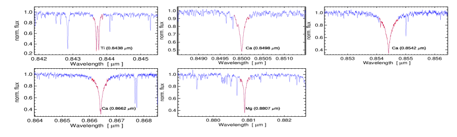
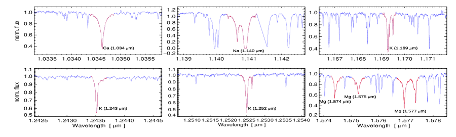
Figure 1: A representation of atomic absorption features in optical (Ti I [0.844 $\mu$m], Ca II [0.850 $\mu$m, 0.854 $\mu$m, 0.866 $\mu$m], Mg I [0.881 $\mu$m]) and Near-infrared (Ca I [1.035 $\mu$m], Na I [1.141 $\mu$m], K I [1.169 $\mu$m, 1.240 $\mu$m, 1.250 $\mu$m], Mg I [1.570 $\mu$m]) for the CARMENES spectra of the M-Dwarf GJ 2 (J00051+457) of spectral type M1.0V. We have calculated the EWs of these features with the feature window shown in red color to find and establish the strongest correlations with the stellar parameters.

3 Result and Discussion :

3.1 Spectroscopic Analysis : Optical and NIR EW estimation

The presence of broad and complex molecular absorption bands in the optical (TiO, VO, CaH) and NIR (H₂O, FeH, CO, OH) over the entire spectral sequence of M dwarfs, make it difficult to identify the weak atomic lines in the spectra. The atomic features, such as Ti I (0.844 $\mu$m), Ca II (0.850 $\mu$m, 0.854 $\mu$m, 0.866 $\mu$m), Mg I (0.881 $\mu$m) in the optical band and the lines Ca I (1.035 $\mu$m), Na I (1.141 $\mu$m), K I (1.169 $\mu$m, 1.240 $\mu$m, 1.250 $\mu$m), Mg I (1.570 $\mu$m) in the NIR are strong enough and comparatively free from any blends and telluric contaminations. These spectral features are ideal tracers of $T_{\rm eff}$, radius, and luminosity as the line strengths or equivalent widths depend on these stellar parameters (Rajpurohit et al. 2018 ; Newton et al. 2015 ). In Fig. 1 we show a representation of the absorption lines in the CARMENES spectra of the object GJ 2 (J00051+457) with the feature window colored in red. Some of the NIR atomic absorption features and indices that show significant correlation with stellar properties like Mg I at 1.50 $\mu$m, Al I at 1.67 $\mu$m, Mg I at 1.71 $\mu$m and $H_{2}O$-H index defined from 1.595 $\mu$m to 1.780 $\mu$m (Newton et al. 2015 ; Khata et al. 2020 ) are absent in the analysis as they are completely or partially in the gap of the CARMENES spectral format. In the J- band region, from 1.20 $\mu$m to 1.48 $\mu$m, the two K I lines at 1.243 $\mu$m and 1.252 $\mu$m stand out prominently, but the rest of this region is very poor in absorption lines due to wide molecular absorptions, telluric $O_{2}$ absorption and strong $H_{2}O$ opacity. We have measured the EWs of the selected lines using the standard equation :

$$\hskip 71.13188ptEW_{\lambda}=\int_{\lambda 1}^{\lambda 2}[1-\frac{F(\lambda)}{F_{c}(\lambda)}]d\lambda$$ (1)

Table 1: Optical and NIR spectral features and continuum points

Feature	Feature window	Blue Continuum	Red Continuum
	($\mu$m)	($\mu$m)	($\mu$m)
Ti I (0.844 $\mu$m)a	0.8436   0.8440	0.8431   0.8436	0.8443   0.8448
Ca II (0.850 $\mu$m)a	0.8498    0.8504	0.8485   0.8496	0.8504   0.8512
Ca II (0.854 $\mu$m)a	0.8540   0.8550	0.8530   0.8539	0.8552   0.8560
Ca II (0.866 $\mu$m)a	0.8660   0.8670	0.8650   0.8660	0.8670   0.8676
Mg I (0.881 $\mu$m)a	0.8808   0.8812	0.8798    0.8803	0.8815    0.8822
Ca I (1.034 $\mu$m)a	1.0343   1.0350	1.0335   1.0341	1.0352    1.0358
Na I (1.140 $\mu$m)b	1.1404   1.1413	1.1389   1.1397	1.1425    1.1434
K I (1.169 $\mu$m)b	1.1691    1.1697	1.1686    1.1691	1.1697    1.1705
K I (1.243 $\mu$m)b	1.2433    1.2438	1.2427    1.2433	1.2438    1.2444
K I (1.252 $\mu$m)b	1.2523   1.2528	1.2513   1.2520	1.2529    1.2535
Mg I (1.574 $\mu$m)b	1.5740    1.5780	1.5720   1.5740	1.5780   1.5800

Notes. Wavelengths are given in vacuum; ^(a) Atomic features are identified in Reiners et al. (2018 ), feature and continuum windows are defined based on our observations; ^(b) Feature and continuum windows are modified from those defined in Newton et al. (2015 )

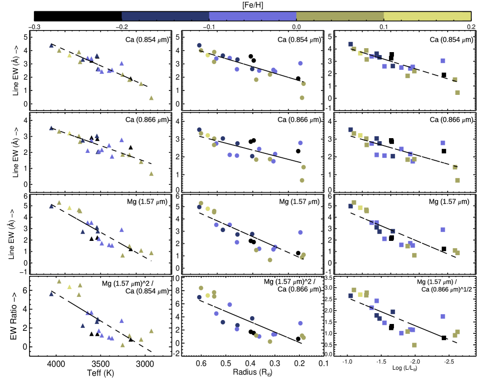
Figure 2: EWs and functional forms of EW ratios in optical and NIR CARMENES spectra that are used to establish best fitting calibration relationships are plotted against the measured $T_{\rm eff}$, radius and luminosity (log L/$L_{\sun}$) for our calibration sample. The data points are color-coded according to the [Fe/H] values taken from Schweitzer et al. (2019 ) and the dashed straight lines represent the linear correlation.

Table 2: Measured EWs of the spectral features from the optical and NIR CARMENES spectra for the interferometric calibration sample.

Star	Ti (0.844 $\mu$m)	Ca (0.850 $\mu$m)	Ca (0.854 $\mu$m)	Ca (0.866 $\mu$m)	Mg (0.881 $\mu$m)	Ca (1.034 $\mu$m)	Na (1.140 $\mu$m)	K (1.169 $\mu$m)	K (1.243 $\mu$m)	K (1.252 $\mu$m)	Mg (1.574 $\mu$m)
	(Å)	(Å)	(Å)	(Å)	(Å)	(Å)	(Å)	(Å)	(Å)	(Å)	(Å)
Gl 172	1.231$\pm$0.105	0.901$\pm$0.007	4.393$\pm$0.310	3.530$\pm$0.202	0.756$\pm$0.030	0.797$\pm$0.022	2.019$\pm$0.018	0.620$\pm$0.015	0.066$\pm$0.017	0.354$\pm$0.011	4.971$\pm$0.246
Gl 208	1.293$\pm$0.055	0.803$\pm$0.004	4.006$\pm$0.145	3.320$\pm$0.107	0.692$\pm$0.017	—	2.340$\pm$0.051	0.689$\pm$0.008	0.188$\pm$0.017	0.512$\pm$0.008	5.283$\pm$0.127
GJ 809	0.573$\pm$0.038	0.796$\pm$0.010	3.887$\pm$0.187	3.028$\pm$0.188	0.696$\pm$0.025	0.817$\pm$0.010	3.770$\pm$0.009	0.986$\pm$0.030	0.258$\pm$0.005	0.451$\pm$0.016	4.644$\pm$0.126
GJ 412A	1.251$\pm$0.026	0.752$\pm$0.007	3.565$\pm$0.147	2.856$\pm$0.381	0.534$\pm$0.019	0.786$\pm$0.005	2.682$\pm$0.021	0.733$\pm$0.024	0.031$\pm$0.013	0.302$\pm$0.017	2.219$\pm$0.106
GJ 15A	1.399$\pm$0.090	0.760$\pm$0.026	3.253$\pm$0.430	2.926$\pm$0.275	0.463$\pm$0.025	0.822$\pm$0.020	3.219$\pm$0.018	0.866$\pm$0.016	0.191$\pm$0.021	0.375$\pm$0.010	2.123$\pm$0.218
GJ 649	1.283$\pm$0.029	0.794$\pm$0.009	3.399$\pm$0.263	2.753$\pm$0.211	0.335$\pm$0.011	0.887$\pm$0.017	3.646$\pm$0.014	0.947$\pm$0.025	0.245$\pm$0.017	0.459$\pm$0.006	3.523$\pm$0.035
GJ 205	1.439$\pm$0.052	0.867$\pm$0.005	3.656$\pm$0.174	3.209$\pm$0.121	0.631$\pm$0.016	—	4.125$\pm$0.027	1.120$\pm$0.027	0.310$\pm$0.012	0.546$\pm$0.015	4.829$\pm$0.194
GJ 880	—	0.641$\pm$0.010	3.153$\pm$0.115	2.672$\pm$0.273	0.143$\pm$0.026	0.807$\pm$0.021	4.489$\pm$0.019	1.131$\pm$0.028	0.288$\pm$0.007	0.472$\pm$0.010	4.547$\pm$0.141
GJ 526	1.075$\pm$0.042	0.761$\pm$0.009	3.438$\pm$0.266	2.114$\pm$0.280	0.616$\pm$0.015	0.773$\pm$0.024	3.109$\pm$0.038	0.776$\pm$0.025	0.233$\pm$0.008	0.396$\pm$0.005	3.524$\pm$0.090
GJ 411	0.007$\pm$0.017	0.151$\pm$0.007	2.616$\pm$0.062	2.040$\pm$0.144	0.064$\pm$0.013	—	3.507$\pm$0.010	0.502$\pm$0.023	0.024$\pm$0.008	0.063$\pm$0.012	2.775$\pm$0.027
GJ 176	1.315$\pm$0.071	0.679$\pm$0.009	3.325$\pm$0.240	2.757$\pm$0.141	0.617$\pm$0.022	0.928$\pm$0.028	2.152$\pm$0.027	0.641$\pm$0.029	0.011$\pm$0.013	0.372$\pm$0.010	2.740$\pm$0.261
Gl 104	1.247$\pm$0.180	0.777$\pm$0.020	3.621$\pm$0.455	3.036$\pm$0.314	0.465$\pm$0.049	0.900$\pm$0.012	2.873$\pm$0.025	0.577$\pm$0.045	0.268$\pm$0.018	0.528$\pm$0.014	3.113$\pm$0.099
GJ 436	1.006$\pm$0.075	0.661$\pm$0.012	2.593$\pm$0.197	2.072$\pm$0.578	0.500$\pm$0.025	0.971$\pm$0.012	3.220$\pm$0.011	0.801$\pm$0.012	0.269$\pm$0.023	0.476$\pm$0.009	2.104$\pm$0.079
GJ 581	1.127$\pm$0.062	0.560$\pm$0.010	2.424$\pm$0.461	2.162$\pm$0.308	0.587$\pm$0.017	0.996$\pm$0.010	3.909$\pm$0.016	1.208$\pm$0.068	0.318$\pm$0.014	0.539$\pm$0.042	1.722$\pm$0.293
Gl 109	1.389$\pm$0.075	0.658$\pm$0.015	2.495$\pm$0.221	2.445$\pm$0.224	0.449$\pm$0.037	0.983$\pm$0.011	4.051$\pm$0.023	1.105$\pm$0.019	0.276$\pm$0.014	0.531$\pm$0.008	1.579$\pm$0.093
GJ 628	—	0.390$\pm$0.011	2.548$\pm$0.303	1.753$\pm$0.182	0.135$\pm$0.010	0.708$\pm$0.031	3.457$\pm$0.029	0.658$\pm$0.069	0.281$\pm$0.026	0.530$\pm$0.018	1.528$\pm$0.212
GJ 273	1.450$\pm$0.065	0.531$\pm$0.008	2.201$\pm$0.263	1.871$\pm$0.156	0.400$\pm$0.020	0.011$\pm$0.010	1.543$\pm$0.013	0.124$\pm$0.009	—	0.056$\pm$0.014	0.666$\pm$0.044
GJ 699	—	—	0.160$\pm$0.290	0.642$\pm$0.159	—	0.260$\pm$0.018	2.087$\pm$0.018	0.025$\pm$0.034	—	0.014$\pm$0.021	1.473$\pm$0.085
GJ 729	1.652$\pm$0.041	0.493$\pm$0.012	1.898$\pm$0.228	2.323$\pm$0.200	0.467$\pm$0.028	1.095$\pm$0.042	4.497$\pm$0.021	1.476$\pm$0.015	0.498$\pm$0.016	0.824$\pm$0.015	1.225$\pm$0.281
GJ 447	1.087$\pm$0.101	0.700$\pm$0.010	3.043$\pm$0.252	2.786$\pm$0.734	0.621$\pm$0.033	0.880$\pm$0.025	2.466$\pm$0.020	0.588$\pm$0.019	0.249$\pm$0.009	0.463$\pm$0.020	2.907$\pm$0.346
GJ 876	1.410$\pm$0.067	0.477$\pm$0.022	1.815$\pm$0.251	1.847$\pm$0.532	0.444$\pm$0.043	0.980$\pm$0.031	4.513$\pm$0.035	1.182$\pm$0.053	0.418$\pm$0.016	0.732$\pm$0.017	1.469$\pm$0.193
Gl 1253	—	0.066$\pm$0.028	1.511$\pm$0.781	1.421$\pm$0.698	0.168$\pm$0.110	0.627$\pm$0.081	3.550$\pm$0.025	0.409$\pm$0.020	0.259$\pm$0.017	0.847$\pm$0.018	1.091$\pm$0.263
Gl 905	—	—	0.456$\pm$0.298	0.679$\pm$0.807	0.135$\pm$0.068	0.594$\pm$0.056	4.048$\pm$0.051	0.251$\pm$0.083	—	0.366$\pm$0.021	0.879$\pm$0.103

Notes. Wavelengths are given in vacuum and the respective feature windows and continuums are given in Table 1 .

Here, $F(\lambda)$ represents the flux across the wavelength range of the line $(\lambda_{2}-\lambda_{1})$, and $F_{c}(\lambda)$ stands for the estimated continuum flux on either side of the absorption line. The EWs are estimated using the modified versions of the publicly available IDL-based tellrv and nirew packages originally developed by Newton et al. (2014 , 2015 ). M dwarf’s spectra are typically polluted by broad absorption features or affected by extinction and contributions from emission sources such as hot dust. So based on our observation, we selected a pseudo continuum for each atomic feature by linear interpolation between adjacent regions, roughly 0.001-0.0015 $\mu$m wide on each side of the absorption line. The features and the continuum points used to calculate the equivalent widths are given in Table 1. The CARMENES high-resolution spectra show all three components of the NIR Mg I triplet (1.5740 $\mu$m, 1.5748 $\mu$m, 1.5765 $\mu$m), and as our continuum window covers all the components, they jointly contribute to the EW estimation of the Mg I (1.57 $\mu$m) feature. We have estimated the uncertainties on the EWs using a Monte Carlo simulation where multiple random realizations of Gaussian noise are added to the spectrum and EWs of the features are recalculated (Khata et al. 2020 ). The estimated EWs along with the associated errors of the spectral features from the optical and NIR CARMENES spectra for our interferometric calibration sample are given in Table 2.

3.2 Spectral features selection: Behavior with stellar parameters

Table 3: Linear Pearson Correlation Coefficient (LPCC) values between the features and stellar parameters for the calibration sample.

				LPCC
Feature		$T_{\rm eff}$ (K)		Radius ($R_{\sun}$)		log (L/$L_{\sun}$)
Ti I (0.844 $\mu$m)		-0.17		-0.12		-0.17
Ca II (0.850 $\mu$m)		+0.70		+0.67		+0.69
Ca II (0.854 $\mu$m)		+0.87		+0.83		+0.86
Ca II (0.866 $\mu$m)		+0.81		+0.75		+0.78
Mg I (0.881 $\mu$m)		+0.55		+0.43		+0.46
Ca I (1.034 $\mu$m)		+0.28		+0.29		+0.31
Na I (1.140 $\mu$m)		-0.23		-0.06		-0.10
K I (1.169 $\mu$m)		+0.26		+0.30		+0.32
K I (1.243 $\mu$m)		-0.49		-0.32		-0.39
K I (1.252 $\mu$m)		-0.15		-0.04		-0.09
Mg I (1.574 $\mu$m)		+0.88		+0.85		+0.82

Notes : Wavelengths are given in vacuum.

We performed a principal component analysis (PCA) to search for the strongest correlations between the EWs of our calibration sample, and we calculated the linear Pearson correlation coefficients (LPCC) looking for legitimate correlation with the EWs and $T_{\rm eff}$, radius, and luminosity. The LPCC value ranges from -1 to +1, and for two variables, such as X and Y, a positive correlation coefficient value indicates Y is increasing as X increases, and a negative value means Y decreases as X increases. We found that the EWs of Ca II (0.854 $\mu$m) and Ca II (0.866 $\mu$m) in the optical channel and the EWs of Mg I (1.574 $\mu$m) in the NIR channel attribute mostly in the first principal components (explaining 79% of the variance) in the PCA test. These three features also give the maximum LPCC values while we investigated for linear correlation with the stellar parameters, and we have given the respective LPCC values of the spectral features in Table 3. These two singly ionized Ca II (0.854 $\mu$m, 0.866 $\mu$m) lines (e.g., Ca II IRT infrared triplet) are prominent features in the spectra of cool M type stars and lie in a region of the spectrum with a well-defined continuum and are significantly free from telluric lines. Earlier work has helped to establish the sensitivity of these lines with stellar atmospheric parameters, such as Mallik (1994 , 1997 ) and Andretta et al. (2005 ) tried to model the behavior of Ca II IRT line strength with $T_{\rm eff}$, log g and metallicity; Zhou (1991 ) showed a significant effect of temperatures on Ca II IRT lines for cooler stars (up to M7) at low $T_{\rm eff}$ and Terrien et al. Terrien2015 (2015) developed a technique to determine M-dwarfs M_k and radius using Ca II IRT feature. Among all the features in the optical and NIR band, Mg I (1.574 $\mu$m) shows the best correlation with the stellar parameters. The EW of the Mg I (1.574 $\mu$m) feature is used by Newton et al. (2015 ) to estimate the stellar radius of M dwarfs in the MEarth sample; Martinez et al. (2017 ) used this feature to calibrate $T_{\rm eff}$ and radius of K- and M-dwarf stars; and later the feature is also used by Khata et al. (2020 ) for the calibration of $T_{\rm eff}$, radius and luminosity of low-resolution M-dwarfs spectra. Therefore, based on the PCA test and the best LPCC values obtained, we selected these three spectral features from the initially considered 11 features for empirical calibrations of the stellar parameters.
      In Fig. 2, we show the plot of the EWs and ratios of EWs for the selected spectral features [i.e., Ca (0.854 $\mu$m), Ca (0.866 $\mu$m), Mg (1.574 $\mu$m)] for the interferometric calibration sample against $T_{\rm eff}$, radius and luminosity. The data points are color-coded by their respective metallicity ([Fe/H]) values as estimated by Schweitzer et al. (2019 ). As the atomic lines get broadened from early to later M dwarfs, the EWs decrease as effective temperature decreases. We see that the EWs of the two Ca II lines and the Mg I line and the line ratios behave almost in a linear fashion, implied by the dashed straight line fittings, as functions of $T_{\rm eff}$, radius and log (L/$L_{\sun}$) with no statistically significant metallicity dependence.

Table 4: Different types of linear trial functions with one example each, using simple functional forms of the selected EWs and EW ratios (x = EW_Ca[0.854μm] ; y = EW_Ca[0.866μm] ; z = EW_Mg[1.574μm]) and associated RMSE, MAD and ${R^{2}}_{ap}$ values of the stellar parameters. The upper case X, Y, Z represent functional forms of x, y, z ( i.e, X = x , $x^{2}$ , $x^{1/2}$ , 1/x , $1/x^{2}$ , $1/x^{1/2}$ ; Y = y , $y^{2}$ , $y^{1/2}$ , 1/y , $1/y^{2}$ , $1/y^{1/2}$ ; Z = z , $z^{2}$ , $z^{1/2}$ , 1/z , $1/z^{2}$ , $1/z^{1/2}$).

			$T_{\rm eff}$ (K)			Radius (${R}_{\odot}$)			log (L/${L}_{\odot}$)
Nature of linear test functions	Example function	RMSE	MAD	${R^{2}}_{ap}$	RMSE	MAD	${R^{2}}_{ap}$	RMSE	MAD	${R^{2}}_{ap}$
single EW, single component [a + bX]	a+bx	147.15	111.90	0.737	0.082	0.062	0.672	0.253	0.174	0.730
single EW, single component [a + bY]	a+by	172.40	140.07	0.638	0.096	0.071	0.547	0.311	0.216	0.591
single EW, single component [a + bZ]	a+bz	137.18	108.68	0.771	0.076	0.055	0.712	0.282	0.216	0.663
single EW, double component [a + bX +c$X^{\prime}$ ($X^{\prime}\subseteq$X; $X^{\prime}\neq$X)]	a+bx+c$x^{2}$	126.75	98.00	0.805	0.078	0.053	0.701	0.249	0.171	0.737
single EW, double component [a + bY +c$Y^{\prime}$ ($Y^{\prime}\subseteq$Y; $Y^{\prime}\neq$Y)]	a+by+c$y^{2}$	166.72	132.76	0.662	0.097	0.066	0.540	0.318	0.215	0.573
single EW, double component [a + bZ +c$Z^{\prime}$ ($Z^{\prime}\subseteq$Z; $Z^{\prime}\neq$Z)]	a+bz+c$z^{2}$	138.66	109.38	0.766	0.078	0.053	0.699	0.283	0.195	0.661
double EWs, double component [a +bX +cY]	a+bx+cy	150.66	112.24	0.724	0.083	0.062	0.663	0.254	0.175	0.726
double EWs, double component [a +bX +cZ]	a+bx+cz	114.20	85.69	0.841	0.069	0.041	0.769	0.230	0.139	0.777
double EWs, double component [a +bY +cZ]	a+by+cz	124.14	98.57	0.812	0.074	0.046	0.730	0.261	0.172	0.712
single EW ratio, single component [a +b$R_{1}$ ($R_{1}$ =X/Y)]	a+bx/y	248.36	191.47	0.250	0.119	0.095	0.299	0.390	0.309	0.357
single EW ratio, single component [a +b$R_{2}$ ($R_{2}$ =X/Z)]	a+bx/z	285.48	209.99	0.008	0.143	0.112	-0.008	0.493	0.383	-0.029
single EW ratio, single component [a +b$R_{3}$ ($R_{3}$ =Y/Z)]	a+by/z	264.92	193.59	0.146	0.134	0.106	0.115	0.466	0.362	0.081
single EW $\&$ single EW ratio, double component [a+bX+c$R_{1}$]	a+bx+cx/y	140.03	110.91	0.761	0.083	0.060	0.662	0.258	0.171	0.719
single EW $\&$ single EW ratio, double component [a+bX+c$R_{2}$]	a+bx+cx/z	128.86	100.45	0.798	0.077	0.052	0.710	0.246	0.159	0.745
single EW $\&$ single EW ratio, double component [a+bX+c$R_{3}$]	a+bx+cy/z	128.28	101.01	0.800	0.076	0.053	0.715	0.241	0.156	0.753
single EW $\&$ single EW ratio, double component [a+bY+c$R_{1}$]	a+by+cx/y	173.69	133.40	0.633	0.094	0.072	0.566	0.296	0.208	0.629
single EW $\&$ single EW ratio, double component [a+bY+c$R_{2}$]	a+by+cx/z	159.53	124.71	0.690	0.093	0.064	0.574	0.309	0.204	0.596
single EW $\&$ single EW ratio, double component [a+bY+c$R_{3}$]	a+by+cy/z	143.75	109.19	0.749	0.087	0.057	0.631	0.288	0.185	0.648
single EW $\&$ single EW ratio, double component [a+bZ+c$R_{1}$]	a+bz+cx/y	130.58	101.53	0.793	0.070	0.048	0.758	0.245	0.174	0.745
single EW $\&$ single EW ratio, double component [a+bZ+c$R_{2}$]	a+bz+cx/z	124.47	98.52	0.811	0.070	0.044	0.762	0.246	0.172	0.744
single EW $\&$ single EW ratio, double component [a+bZ+c$R_{3}$]	a+bz+cy/z	132.00	105.23	0.788	0.074	0.049	0.733	0.268	0.197	0.697
single EW ratio, double component [a +bR1 +cR${}_{1}^{\prime}$ (R${}_{1}^{\prime}\neq R_{1}$)]	a+bx/y+cx/$y^{2}$	181.69	138.02	0.598	0.100	0.078	0.507	0.305	0.222	0.605
single EW ratio, double component [a +bR2 +cR${}_{2}^{\prime}$ (R${}_{2}^{\prime}\neq R_{2}$)]	a+bx/z+cx/$z^{2}$	261.95	196.47	0.165	0.136	0.111	0.082	0.453	0.362	0.131
single EW ratio, double component [a +bR3 +cR${}_{3}^{\prime}$ (R${}_{3}^{\prime}\neq R_{3}$)]	a+by/z+cy/$z^{2}$	262.06	189.85	0.164	0.136	0.104	0.093	0.464	0.352	0.088
double EW ratio, double component [a + bR1 + cR2]	a+bx/y+cx/z	222.67	168.38	0.397	0.108	0.085	0.426	0.361	0.282	0.447
double EW ratio, double component [a + bR1 + cR3]	a+bx/y+cy/z	220.25	165.42	0.410	0.108	0.084	0.429	0.359	0.274	0.455
double EW ratio, double component [a + bR2 + cR3]	a+bx/z+cy/z	229.74	171.63	0.358	0.116	0.093	0.335	0.385	0.299	0.372
Accepted linear functions for $T_{eff}$ (${\star}$), Radius (${\dagger}$) and Luminosity (${\mathsection}$) respectively with minimum RMSE and maxmimum ${R^{2}}_{ap}$ values
(${\star}$) single EW $\&$ single EW ratio, double component	a+bx+c$z^{2}$/x	99.00	70.97	0.881
(${\dagger}$) single EW $\&$ single EW ratio, double component	a+bx+c$z^{2}$/y				0.067	0.043	0.779
(${\mathsection}$) double EW ratio, double component	a+bz/$\sqrt{y}$+cx/$\sqrt{z}$							0.218	0.137	0.798

Notes. Table 4 is available in its entirety in the electronic version of the journal as supplementary material.

Figure 3: A representation of the estimated RMSE, MAD and $R^{2}_{ap}$ (plotted along the y-axes) of the different trial functions (plotted along the x-axes going from 1 to 8001) for $T_{\rm eff}$ (left panel, blue color), radius (middle panel, cyan color) and log luminosity (right panel, olive color) is shown here. The respective RMSE, MAD and $R^{2}_{ap}$ values of the chosen best fitting functions are marked by orange circles and the lowest values of RMSE and MAD and the highest value of $R^{2}_{ap}$ are represented by the red star symbols.

3.3 Empirical Calibrations of $T_{\rm eff}$, radius and luminosity

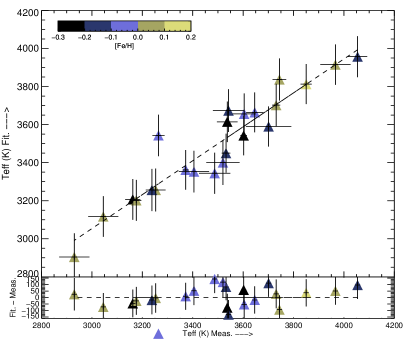
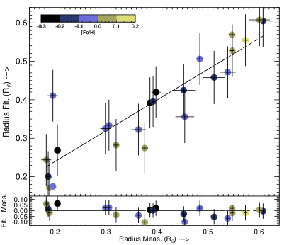
Figure 4: We show the plots of our best-fitting calibration relationships and the respective residuals for $T_{\rm eff}$ (filled triangles in the top left panel), radius (filled circles in the top right panel), and Log ($L_{bol}$) (filled squares in bottom panel) here. The horizontal axes show the directly measured stellar parameters taken from Boyajian et al. (2012 ), Mann et al. (2013b , 2015 ) and Markus Rabus et al. (2019 ). In the top plot of each panel, the vertical axes represent the stellar parameters inferred from the best fits of this work; and in the lower plot of each panel, the vertical axes represent the residuals between the best-fitting values and the measured values. The data points are color-coded by the [Fe/H] values from Schweitzer et al. (2019 ).

Table 5: Inferred $T_{\rm eff}$, radius and $L_{bol}$ for the calibration sample.

Star			Teff (K)			Radius ($R_{\sun}$)			log $L/L_{\sun}$
		Measured	Inferred (e)		Measured	Inferred (f)		Measured	Inferred (g)
Gl 172 a		4054$\pm$38	3957$\pm$108		0.608$\pm$0.020	0.604$\pm$0.067		–1.048$\pm$0.009	–1.12$\pm$0.23
Gl 208 a		3966$\pm$60	3915$\pm$106		0.601$\pm$0.020	0.608$\pm$0.068		–1.097$\pm$0.010	–1.10$\pm$0.23
GJ 809 b		3744$\pm$27	3837$\pm$111		0.547$\pm$0.006	0.569$\pm$0.067		–1.280$\pm$0.005	–1.19$\pm$0.22
GJ 412A b		3537$\pm$41	3615$\pm$107		0.398$\pm$0.009	0.420$\pm$0.067		–1.655$\pm$0.004	–1.63$\pm$0.22
GJ 15A b		3602$\pm$13	3542$\pm$104		0.386$\pm$0.002	0.392$\pm$0.066		–1.647$\pm$0.005	–1.75$\pm$0.22
GJ 649 d		3604$\pm$46	3657$\pm$107		0.539$\pm$0.015	0.472$\pm$0.067		–1.359$\pm$0.002	–1.48$\pm$0.22
GJ 205 b		3850$\pm$22	3813$\pm$105		0.574$\pm$0.004	0.555$\pm$0.067		–1.190$\pm$0.009	–1.25$\pm$0.22
GJ 880 b		3731$\pm$16	3703$\pm$112		0.548$\pm$0.004	0.528$\pm$0.068		–1.286$\pm$0.004	–1.29$\pm$0.23
GJ 526 b		3646$\pm$34	3664$\pm$105		0.484$\pm$0.008	0.506$\pm$0.067		–1.433$\pm$0.006	–1.31$\pm$0.22
GJ 411 b		3532$\pm$17	3450$\pm$103		0.392$\pm$0.003	0.395$\pm$0.066		–1.671$\pm$0.006	–1.70$\pm$0.22
GJ 176 d		3701$\pm$90	3590$\pm$106		0.453$\pm$0.022	0.425$\pm$0.067		–1.475$\pm$0.003	–1.64$\pm$0.22
Gl 104 a		3542$\pm$62	3674$\pm$112		0.512$\pm$0.022	0.458$\pm$0.069		–1.432$\pm$0.012	–1.54$\pm$0.23
GJ 436 b		3520$\pm$66	3401$\pm$118		0.455$\pm$0.018	0.356$\pm$0.068		–1.548$\pm$0.011	–1.85$\pm$0.23
GJ 581 b		3487$\pm$62	3344$\pm$108		0.299$\pm$0.010	0.325$\pm$0.067		–1.928$\pm$0.007	–1.97$\pm$0.22
Gl 109 a		3405$\pm$60	3353$\pm$110		0.364$\pm$0.014	0.323$\pm$0.067		–1.797$\pm$0.015	–1.99$\pm$0.23
GJ 628 c		3372$\pm$12	3362$\pm$104		0.306$\pm$0.007	0.334$\pm$0.066		–1.965$\pm$0.070	–1.88$\pm$0.22
GJ 273 c		3253$\pm$39	3256$\pm$113		0.320$\pm$0.005	0.282$\pm$0.068		–1.988$\pm$0.102	–1.92$\pm$0.23
GJ 699 b		3238$\pm$11	3256$\pm$111		0.187$\pm$0.001	0.200$\pm$0.066		–2.466$\pm$0.003	–2.46$\pm$0.22
GJ 729 c		3162$\pm$30	3207$\pm$107		0.205$\pm$0.006	0.269$\pm$0.067		–2.424$\pm$0.169	–2.24$\pm$0.22
GJ 447 c		3264$\pm$24	3543$\pm$109		0.196$\pm$0.010	0.411$\pm$0.067		–2.408$\pm$0.198	–1.70$\pm$0.23
GJ 876 d		3176$\pm$20	3202$\pm$107		0.376$\pm$0.005	0.275$\pm$0.067		–1.889$\pm$0.002	–2.19$\pm$0.23
GL 1253 a		3045$\pm$60	3117$\pm$107		0.183$\pm$0.009	0.244$\pm$0.067		–2.588$\pm$0.047	–2.31$\pm$0.23
Gl 905 a		2930$\pm$60	2904$\pm$125		0.189$\pm$0.007	0.171$\pm$0.069		–2.626$\pm$0.041	–2.70$\pm$0.23

Notes. Interferometrically measured parameters are taken from ^a Mann et al. (2015 ) ; ^b Newton et al. (2015 ) ; ^c Markus Rabus et al. (2019 ) ; ^d Mann et al. (2013b ). ^(e) $T_{\rm eff}$ is inferred using equation (2), the fitting is shown in Fig. 4, top left panel ; ^(f) Radius is inferred using equation (3), the fitting is shown in Fig. 4, top right panel ; ^(g) log $L/L_{\sun}$ is inferred using equation (4), the fitting is shown in Fig. 4, bottom panel.

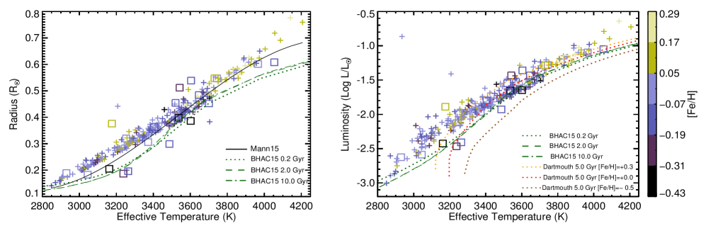
Figure 5: Stellar radius vs. effective temperature (left panel) and luminosity vs. effective temperature (right panel) plot, showing parameter values of CARMENES M-dwarfs (plus symbols) estimated using EW dependent calibration relations and measured values of interferometric calibrators (open square symbols). For the radius vs $T_{\rm eff}$ plot, we overplot the best-fit radius-temperature relation (solid black line) from Mann15 (Mann et al. 2015 ) and 0.2 Gyr, 2.0 Gyr and 10.0 Gyr isochrones (represented by green dotted, dashed and dash-dot lines respectively) for [Fe/H] = 0.0 and log g $\approx$ 5.0 from BHAC15 (Baraffe et al. 2015 ). For the luminosity-$T_{\rm eff}$ plot, we also show the isochrones from BHAC15 along with the 5 Gyr Dartmouth isochrones for [Fe/H] = 0.3 (dotted orange line), [Fe/H] = 0.0 (dotted red line) and [Fe/H] = - 0.5 (dotted brown line). The data points are color-coded by metallicity from Schweitzer et al. (2019 ).

Figure 6: The distribution of estimated $T_{\rm eff}$ (2849 < $T_{\rm eff}$(K) < 4206 ), radius (0.141 < $R/R_{\sun}$ < 0.776) and luminosity (–3.00 < log $L/L_{\sun}$ < –0.643) of the CARMENES M-dwarfs are shown here.

While looking for the best-fit calibration relations, we found that simple linear functions of EWs or ratios of EW give better results than any higher order polynomial functions (e.g, Hoerl function [a$b^{r}*r^{c}$], power law [a$r^{b}$ ; b > 2], exponential [a$b^{r}$], logarithmic [a + b ln(r)] ; r = EW or ratio of EW). The same kind of linear fits are also observed in the work of Newton et al. (2015 ) but unlike them we did not restrict our fits to only the optical or NIR regions, rather we performed a comprehensive search by combining features from both bands simultaneously. For single-line EWs (we used lower case x, y, z as EWs: x = EW_Ca[0.854μm] ; y = EW_Ca[0.866μm] ; z = EW_Mg[1.574μm]), we tested with single component linear functions (e.g., a + bX ; a + bY ; a + bZ), where we used upper case X, Y, Z as simple functional forms of x, y, z ( i.e, X = x , $x^{2}$ , $x^{1/2}$ , 1/x , $1/x^{2}$ , $1/x^{1/2}$ ; Y = y , $y^{2}$ , $y^{1/2}$ , 1/y , $1/y^{2}$ , $1/y^{1/2}$ ; Z = z , $z^{2}$ , $z^{1/2}$ , 1/z , $1/z^{2}$ , $1/z^{1/2}$). We also did test single line double component functions (e.g., a + bX +c$X^{\prime}$ [$X^{\prime}\subseteq$ X ; $X^{\prime}\neq$ X] ; a + bY +c$Y^{\prime}$ [$Y^{\prime}\subseteq$ Y ; $Y^{\prime}\neq$ Y] ; a + bZ +c$Z^{\prime}$ [$Z^{\prime}\subseteq$ Z ; $Z^{\prime}\neq$ Z]). We noticed that the use of more than two components in the linear relation did not give statistically better results, so we limited our test functions to a maximum of two components of EWs or ratio of EWs or combination of both. The multi-line functions (two components) that we tested are : a + bX +cY ; a + bX +cZ ; a + bY +cZ . The ratio of the spectral line depths or equivalent widths (R = EW₁ / EW₂) are found to be very sensitive temperature indicators (Kovtyukh et al. 2003 ) and tracers of other fundamental parameters with high efficiency and accuracy. So we also checked with all possible combinations of EW ratios of the three lines ( R₁ = X / Y ; R₂ = X / Z ; R₃ = Y / Z). For single-ratio (one component) linear functions we did test : a + R_ib (i = 1,2,3), and single-line and single-ratio functions we tested : a + bX + cR_i ; a + bY + cR_i ; a + bZ + cR_i (i =1,2,3) . Like the single-line double component functions, we tried out with single-ratio double component functions : a + bR_i + cR${}_{i}^{\prime}$ (R${}_{i}^{\prime}\subseteq R_{i}$ ; R${}_{i}^{\prime}\neq R_{i}$ ; i = 1,2,3) and also tested with multi-ratio functions : a + bR₁ + cR₂ ; a + bR₁ + cR₃ ; a + bR₂ + cR₃ .
      To find the best-fitting parameters from all possible combinations of linear functional relations, we performed multivariate linear regression and used the adjusted square of the multiple correlation coefficient ($R^{2}_{ap}$ , Rojas-Ayala et al. 2012 ), the root mean squared error (RMSE) and the mean absolute deviation (MAD) values to statistically compare the goodness of each fit. We show the calculations of RMSE, MAD and $R^{2}_{ap}$ as equation (5), equation (6) and equation (7) in the appendix section. For a given set of calibration data, the $R^{2}_{ap}$ shows the proportion of variability in a data set that is accounted for by a regression model (an $R^{2}_{ap}$ value closer to 1 means a superior fit) and the RMSE (a lower RMSE means a better fit) evaluates the accuracy and predictive power of the response of the regression model (Khata et al. 2020 ). We tested 8001 possible combinations of linear trial functions using the selected EWs and EW ratios and in Table 4 we show different types of linear trial functions with one example each, alongwith the respective RMSE, MAD and $R^{2}_{ap}$ values for $T_{\rm eff}$, radius and luminosity. In the case of RMSE, the individual errors are squared and the RMSE gives relatively high weight to large errors, whereas for MAD the errors are co-added in a linear fashion attributing equal weightage on small and large errors. This means the RMSE is more suitable when large deviation from the mean is particularly undesirable. Also as our estimated errors on the EWs are expected to be Gaussian in nature, the RMSE is more appropriate to represent a model performance than the MAD. So we selected the best fitting calibration relations for the stellar parameters mainly on the basis of highest $R^{2}_{ap}$ and lowest RMSE values. To get a clear understanding of how much better the chosen relations are than the rest of the trial functions, we show a representation of the RMSE, MAD and $R^{2}_{ap}$ values in Fig. 3. We find that for $T_{\rm eff}$, our chosen function also gives the lowest MAD value alongside the lowest RMSE value, but for the best fitting radius ($MAD_{rad}$ = 0.043) and luminosity ($MAD_{lum}$ = 0.137) relations the MAD values are slightly greater than the lowest estimated values ($MAD_{lowest,rad}$ = 0.040 and $MAD_{lowest,lum}$ = 0.124). The selected calibration relations for the stellar parameters are given as :

$$\begin{split}\hskip 14.22636pt\textbf{T}_{eff}/K&=\ A+B\times Ca(0.854\mu m)+C\times\frac{[Mg(1.57\mu m)]^{2}}{Ca(0.854\mu m)}\\ \end{split}$$ (2)

A = 2738.37 $\pm$ 39.5 ; B = 232.046 $\pm$ 7.6 ; C = 35.462 $\pm$ 2.6
        $R^{2}_{ap}$ = 0.881 ;     RMSE ($T_{\rm eff}$/K) = 99.0 ;     MAD / K = 71.0

$$\begin{split}\hskip 17.07182pt\textbf{R}/R_{\odot}\ &=\ A+B\times Ca(0.854\mu m)+C\times\frac{[Mg(1.57\mu m)]^{2}}{Ca(0.866\mu m)}\\ \end{split}$$ (3)

A = 0.1102 $\pm$ 0.01 ; B = 0.0757 $\pm$ 0.002 ; C = 0.0231 $\pm$ 0.0009
       $R^{2}_{ap}$ = 0.779 ;   RMSE ($R/R_{\sun}$) = 0.067 ;   MAD / $R_{\sun}$ = 0.043

$$\begin{split}log\textbf{L}/L_{\odot}\ &=\ A+B\times\frac{Ca(0.854\mu m)}{[Mg(1.57\mu m)]^{1/2}}+C\times\frac{Mg(1.57\mu m)}{[Ca(0.866\mu m)]^{1/2}}\\ \end{split}$$ (4)

A = –3.5063 $\pm$ 0.032 ; B = 0.4896 $\pm$ 0.004 ; C = 0.5363 $\pm$ 0.003
     $R^{2}_{ap}$ = 0.798 ;   RMSE ($logL/L_{\sun}$) = 0.218 ;   MAD / dex = 0.137

We show the plots of our best-fitting linear relationships and the respective residuals of the parameters for the calibrator stars in Fig. 4. The final errors on the stellar parameters are estimated by combining the randomly generated Gaussian error propagated from the EWs of the features with the intrinsic scatter (RMSE) inherent in the calibration relations. In Table 5, we present the inferred stellar parameters with associated errors that we estimated using the calibration relations. For our work, we notice that along with the EWs, the simple functional form of the ratios of EWs plays an important role in the calibration. In principle, the change in EWs with $T_{\rm eff}$ for lines with higher excitation potential ($\chi$) should be faster than that for lines with lower ’$\chi$’ and a ratio of EWs should be temperature sensitive if the excitation potential of the lines differs by as much as possible (Gray 1994). The excitation potential of the Ca II IRT lines are 1.70 eV and 1.69 eV, respectively, and for the Mg I triplet, the ’$\chi$’ value is around 5.93 eV, so the EW ratios $Mg(1.57\mu m)/Ca(0.854\mu m)$ and $Mg(1.57\mu m)/Ca(0.866\mu m)$ show better correlation with the stellar parameters than the ratio of the two Ca II IRT lines [i.e., $Ca(0.854\mu m)/Ca(0.866\mu m)$]. Also as the EWs show very negligible metallicity dependence within the parameter-space, selecting the lines from different part of the spectra does not hamper the calibration substantially.
    In Fig. 5, we show the $T_{\rm eff}$-radius (left panel) and $T_{\rm eff}$-luminosity (right panel) distribution of our sample of the CARMENES M-dwarfs. For comparison, in the left panel, we overplot the radius-temperature relation from Mann et al. (2015 , hereafter Mann15) and new evolutionary models of ages 0.2 Gyr, 2.0 Gyr, and 10.0 Gyr for pre-main sequence and main sequence low-mass stars down to the hydrogen-burning limit for solar metallicity by Baraffe et al. (2015 , hereafter BHAC15). Our estimated radii are a little larger than what is predicted by Mann15’s relation and have a distinct separation from the BHAC15 isochrones. One reason for the disagreement could be that the stellar radii for low-mass stars generally are measured to be larger than model predictions (Boyajian et al. 2012 ). Another reason could be the metallicity dependence of parameters (Newton et al. 2015 ) which is observed in our temperature-radius plane. It can be seen that for $T_{\rm eff}$ < 3700, a large part of our sample is metal poor. In the right panel of Fig. 5, we also show the overplot of the BHAC15 isochrones and the 5 Gyr, Dartmouth isochrones (Dotter et al. 2008 ; Feiden et al. 2011 ) for super-solar ([Fe/H] = +0.30 dex), solar ([Fe/H] = 0.0 dex) and sub-solar ([Fe/H] = -0.50 dex) metallicity. Here also metallicity has a significant effect on the models (as noted by Newton et al. 2015 ), and the Dartmouth models predict that for cool stars, there will be a difference of 1 in absolute magnitude for a star with [Fe/H] = -0.50 dex, compared to another star of same effective temperature with [Fe/H] = +0.30 dex.
      In Table 7, we present the estimated EWs of the selected spectral features that we use for the calibration and the stellar parameters of the CARMENES M-dwarf stars. We also show a plot of the distribution of the stellar parameters of our M-dwarf sample in Fig. 6 with the parameter values ranging $T_{\rm eff}$ (2849 < $T_{\rm eff}$(K) < 4206 ), radius (0.141 < $R/R_{\sun}$ < 0.776) and luminosity (–3.00 < log $L/L_{\sun}$ < –0.643).

3.4 Comparison with literature studies

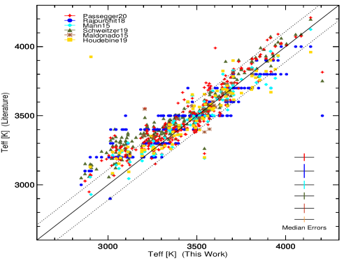
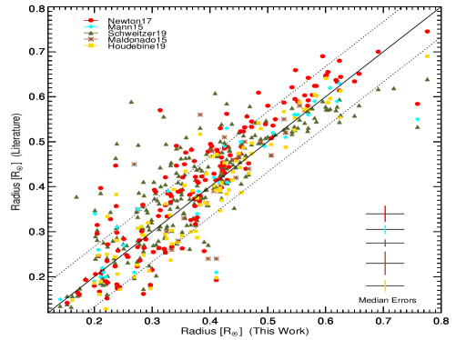
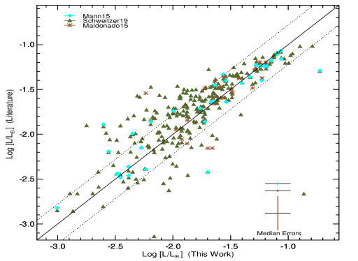
Figure 7: Comparisons of $T_{\rm eff}$ (top panel), radius (middle panel) and luminosity (bottom panel) with literature results (vertical axes) and this work (horizontal axes). The 1:1 relation is indicated by the solid black lines and the dotted lines indicate the typical size of the error bars associated with our work. The median errors associated with the literature values are shown in the lower right corner of each plot. Different determination methods of literature values are indicated by different symbols and colors. Legends used in the plots : Passegger20 (Passegger et al. 2020 ); Rajpurohit18 (Rajpurohit et al. 2018 ); Mann15 (Mann et al. 2015 ); Schweitzer19 (Schweitzer et al. 2019 ); Maldonado15 (Maldonado et al. 2015 ); Houdebine19 (Houdebine et al. 2019 ); Newton17 (Newton et al. 2017 ).

In Fig. 7, we show the comparison of the results that we get in this work (horizontal axes) with the literature parameter values obtained in other works (vertical axes) using different techniques for the overlapping M-dwarfs. In Table 6, we present the median and standard deviation of the differences between the various literature values and the values determined here. For better readability, we do not use error bars in the plots; rather, we show median errors of all the comparisons in the lower right side of each plot.
    In the top panel of Fig. 7, we compare our estimated $T_{\rm eff}$ with different literature works. Passegger et al. (2020 , hereafter Passegger20) derived $T_{\rm eff}$ using neural network architecture for CARMENES spectra, Mann15 calculated $T_{\rm eff}$ by comparing their optical spectra with BT-Settl (PHOENIX) models, Maldonado et al. (2015 , hereafter Maldonado15) used ratios of pseudo EWs of spectral features as temperature diagnostic and Houdebine et al. (2019 , hereafter Houdebine19) used a photometric approach and correlated (R - I)_C color with $T_{\rm eff}$. Apart from some minor scatter, all these results show reasonably good median and standard deviation values of differences with our estimation and overlap (within their error) of the dotted line region which represents $\pm$ 110K from a one-to-one comparison. Comparing the CARMENES spectra with the BT-Settl models both in the optical and in the NIR simultaneously, Rajpurohit et al. (2018 , hereafter Rajpurohit18) estimated $T_{\rm eff}$ with a median error around 100K and Schweitzer et al. (2019 , hereafter Schweitzer19) measured the $T_{\rm eff}$ by fitting the CARMENES spectra of the visual (VIS) channel with PHOENIX-ACES synthetic spectra (Husser et al. 2013 ). Rajpurohit18 and Schweitzer19 show relatively consistent results as the data points stay well within the dotted line region down to 3500K. Below 3500K some of the estimated $T_{\rm eff}$ values (from Rajpurohit18 and Schweitzer19) are up to 300K higher than our values. Although for both the cases, the overall median and standard deviation in differences are less than 90K.
     The comparison of the radius is shown in the middle panel of Fig. 7. Newton et al. (2017 , hereafter Newton17) and Mann15 empirically calibrated stellar radius, Maldonado15 used photometric estimates of radius to calibrate empirical relations using temperatures and metallicities, and Houdebine19 used V-band absolute magnitude and $T_{\rm eff}$ to determine the radii. We observe that the radii estimated by Newton17 and Houdebine19 are larger than our values down to 0.3R_☉ and for radii smaller than that, their values are slightly lower than ours. Schweitzer19 has the biggest scatter (compared to our results), with radii that are generally slightly larger than ours. These discrepancies might be related to the activity level of M-dwarfs (Morales, Ribas and Jordi 2008 ) as either strong magnetic fields predictably inhibiting convection or flux conservation in a magnetic spot-covered stellar surface (López-Morales $\&$ Ribas 2005 ) causes larger radii for a given $T_{\rm eff}$. Also, Schweitzer19 used effective temperature to calculate the radii using Stefan-Boltzmann’s law while they derived their $T_{\rm eff}$ by fitting with synthetic spectra, and experimental evidence suggests that theoretical models have limitations to describe star’s $T_{\rm eff}$ accurately for a value lower than 4000K and that could add errors in radii. However, despite the scatter, the literature radii show consistency with our estimations with the median and standard deviation of differences being well below the median value of our radius uncertainty (0.067 R_☉).
     In the bottom panel of Fig. 7, we show the luminosity comparison for three literature results: Mann15 estimated luminosity using empirical relations, using apparent magnitudes and distances, Schweitzer19 photometrically determined luminosity, and Maldonado15 used the Stefan-Boltzmann law. In general Schweitzer19 is in good agreement with the one-to-one relationship, however there is some scatter in the luminosity (log L/$L_{\sun}$) in the range of -1.5 to -2.0 dex. This mismatch could arise from the discrepancy in the value of the apparent magnitudes as experimental evidence suggests that active and inactive M dwarfs define different sequences in the luminosity-color plane (Stauffer $\&$ Hartmann 1986 ) plane and the uncertainty of distance calculation adds to the inconsistency.

Table 6: Median and standard deviation (Std. Dev.) of differences between the results of literature and this work for stellar parameters

		Median / Std. Dev.
Literature	$T_{\rm eff}$ (K)	Radius ($R_{\sun}$)	log (L/$L_{\sun}$)
Schweitzer et al. (2019 )	75 / 80	0.038 / 0.050	0.13 / 0.22
Maldonado et al. (2015 )	33 / 75	0.025 / 0.056	0.064 / 0.179
Mann et al. (2015 )	45 / 60	0.019 / 0.052	0.10 / 0.19
Houdebine et al. (2019 )	58 / 63	0.012 / 0.055	–
Passegger et al. (2020 )	73 / 69	–	–
Rajpurohit et al. (2018 )	83 / 86	–	–
Newton et al. (2017 )	–	0.043 / 0.045	–

4 Summary and Conclusion

We have estimated effective temperature, radius, and luminosity (L/${L}_{\odot})$ with individual error bars for a sample of 271 M-dwarf stars with spectral types (M0V-M7V) observed in the CARMENES radial-velocity planet survey. We establish new empirical calibration relationships to determine fundamental parameters of low mass M-dwarf stars using EWs and EW ratios of spectral absorption features taken simultaneously from high resolution (R$\sim 90000$) optical (0.52–0.96 $\mu$m) and near-infrared (0.96–1.71 $\mu$m) spectra. The estimation of our physical properties is mostly model-independent, and the main results are summarized as follow:

1. The optical and NIR spectra of CARMENES M-dwarfs contain several important spectral absorption features, which show a legitimate strong correlation with the physical parameters. We select a sample of 23 stars with interferometrically measured radii as our calibrators. We perform principal component analysis (PCA), looking for the strongest correlations among the measured EWs of our calibration sample and derive the linear Pearson correlation coefficient to identify the most suitable tracers of the stellar parameters.

2. The optical (Ca II at 0.854 $\mu$m, Ca II at 0.866 $\mu$m) and NIR (Mg I at 1.574 $\mu$m) features show a strong correlation with the stellar parameters giving the best correlation coefficient values. We find that the absorption lines of low and high excitation potentials ($\chi$) respond differently to the change of stellar parameters and the inclusion of the ratio of the equivalent widths with different excitation potentials in the calibration relations gives comparatively superior results.

3. We investigate simple parameterizations of two EWs or EW ratios or a combination of both and examine every possible single line or multiline linear function. We have performed multivariate linear regression to determine the best fitting parameters and use the adjusted square of the multiple correlation coefficient ($R^{2}_{ap}$), the RMSE, and the mean absolute deviation (MAD) values to statistically compare the goodness of each fit.

4. We notice that the simultaneous use of the EWs and ratios of EWs of these selected features from both the optical and NIR band give the best fit linear calibration relationships of $T_{\rm eff}$, radius, and luminosity with the RMSE values of 99K, 0.06${R}_{\odot}$ and 0.22 dex respectively. Our parameter values cover ranges in the parameter-space of (2849 < $T_{\rm eff}$(K) < 4206 ), (0.141 < $R/R_{\sun}$ < 0.776) and (–3.00 < log $L/L_{\sun}$ < –0.643). The radii and luminosities derived in this work are found to be larger than what is predicted by the theoretical evolutionary models and show some metallicity dependence as we see for $T_{\rm eff}$ < 3700 K, where our sample is mostly metal poor.

5. We also explore and compare our results with literature values obtained with other methods where available. Though the comparison plots display little differences in terms of the median and standard deviation values, the overall agreement is good. Our calibrations can be very useful for understanding the properties of potential planet-host candidates and distant cool stars without parallaxes and flux calibrated spectra.

5 Acknowledgements

The authors are grateful to the reviewer for all the valuable comments and suggestions, which helped to improve the overall quality of this paper. The work is supported by S. N. Bose National Centre for Basic Sciences under the Department of Science and Technology (DST), Govt. of India. The research work leading to this publication has received funding from the INSPIRE Fellowship scheme by the DST, Govt. of India. The result of this research is "Based on data from the CARMENES data archive at CAB (INTA-CSIC)." The authors acknowledge the use of the SIMBAD and VizieR database, operated at CDS, Strasbourg, France. This research made use of the IDL-based tellrv and nirew packages developed by E. R. Newton.

6 Data Availability

All the observational data that we have used for the research work of this paper are publicly available in the CARMENES data archive at CAB (INTA-CSIC) (http://carmenes.cab.inta-csic.es/gto/jsp/reinersetal2018.jsp). Table 4 is available in its entirety as online supplementary material in the journal.

Appendix A Calculations of RMSE, MAD and $R^{2}_{ap}$

The root mean squared error (RMSE) is the square root of the variance of the residuals. The RMSE is defined as :

$$\hskip 56.9055ptRMSE=\sqrt{\sum\limits_{i=1}^{n}\frac{(\widehat{y_{i}}-y_{i})^{2}}{(n-p)}}\\$$ (5)

where, n is the number of data points (i.e., number of calibrators), p is the number of predictors used in the model, $y_{i}$ is the value of the response variable i, and $\widehat{y_{i}}$ is the value predicted by the regression model for given $y_{i}$.

The mean absolute deviation (MAD) measures the statistical dispersion or variability in a dataset. The MAD is defined as :

$$\hskip 71.13188ptMAD=\sum\limits_{i=1}^{n}\frac{|y_{i}-\bar{y}|}{n}\\$$ (6)

where, $\bar{y}$ is the overall mean of the observations $y_{i}$.

The adjusted square of the multiple correlation coefficient ($R^{2}_{ap}$) represents the proportion of variability in a data set that is accounted for by a regression model. The $R^{2}_{ap}$ is defined as :

$$\hskip 56.9055ptR^{2}_{ap}=1-\frac{(n-1)\sum\limits_{i=1}^{n}(\widehat{y_{i}}-y_{i})^{2}}{(n-p)\sum\limits_{i=1}^{n}(y_{i}-\bar{y_{i}})^{2}}\\$$ (7)

Appendix B TABLES

Table 7: EWs of the selected spectral features and estimated stellar parameters of the CARMENES M-dwarf stars.

Karmn(a)	Name	Sp.type(b)	Ca I EW (${\AA}$)	Ca I EW (${\AA}$)	Mg I EW (${\AA}$)	$T_{eff}^{(c)}$	Radius(c)	Luminosity(c)
			(0.854 $\mu$m)	(0.866 $\mu$m)	(1.57 $\mu$m)	(K)	($R_{\sun}$)	(log $L/L_{\sun}$)
J00051+457	GJ 2	M1.0 V	3.491$\pm$0.608	2.426$\pm$0.375	3.761$\pm$0.193	3692$\pm$107	0.509$\pm$0.067	–1.330$\pm$0.224
J00067-075	GJ 1002	M5.5 V	0.577$\pm$0.555	1.368$\pm$0.355	0.590$\pm$0.130	2894$\pm$129	0.160$\pm$0.069	–2.868$\pm$0.232
J00162+198E	GJ 1006B	M4.0 V	1.022$\pm$0.505	1.452$\pm$0.311	1.060$\pm$0.294	3015$\pm$108	0.205$\pm$0.067	–2.548$\pm$0.224
J00183+440	GJ 15A	M1.0 V	3.253$\pm$0.430	2.926$\pm$0.275	2.123$\pm$0.218	3542$\pm$104	0.392$\pm$0.066	–1.747$\pm$0.222
J00184+440	GJ 15B	M3.5 V	2.400$\pm$0.523	2.272$\pm$0.320	0.730$\pm$0.192	3303$\pm$110	0.297$\pm$0.067	–1.871$\pm$0.226
J00286-066	GJ 1012	M4.0 V	1.750$\pm$0.598	1.824$\pm$0.394	1.856$\pm$0.353	3214$\pm$128	0.286$\pm$0.071	–2.140$\pm$0.241
J00389+306	GJ 26	M2.5 V	3.145$\pm$0.297	2.314$\pm$0.205	2.723$\pm$0.142	3552$\pm$110	0.422$\pm$0.067	–1.613$\pm$0.226
J00570+450	G 172-030	M3.0 V	1.908$\pm$0.511	2.634$\pm$0.321	1.458$\pm$0.138	3221$\pm$141	0.273$\pm$0.072	–2.251$\pm$0.250
J01013+613	GJ 47	M2.0 V	2.826$\pm$0.479	2.237$\pm$0.318	2.326$\pm$0.087	3462$\pm$119	0.380$\pm$0.068	–1.765$\pm$0.232
J01025+716	GJ 48	M3.0 V	2.500$\pm$0.259	2.417$\pm$0.190	2.676$\pm$0.245	3420$\pm$103	0.368$\pm$0.066	–1.835$\pm$0.221
J01026+623	GJ 49	M1.5 V	3.699$\pm$0.251	3.031$\pm$0.176	3.797$\pm$0.057	3735$\pm$104	0.500$\pm$0.066	–1.407$\pm$0.221
J01048-181	GJ 1028	M5.0 V	0.459$\pm$0.728	0.965$\pm$0.461	0.585$\pm$0.200	2871$\pm$126	0.153$\pm$0.067	–2.893$\pm$0.223
J01125-169	GJ 54.1	M4.5 V	0.662$\pm$0.690	1.780$\pm$0.355	0.388$\pm$0.117	2900$\pm$108	0.162$\pm$0.067	–2.830$\pm$0.224
J01339-176	LP 768-113	M4.0 V	1.150$\pm$0.802	1.534$\pm$0.458	1.128$\pm$0.226	3044$\pm$118	0.216$\pm$0.069	–2.487$\pm$0.233
J01433+043	GJ 70	M2.0 V	3.167$\pm$0.578	2.732$\pm$0.302	2.809$\pm$0.219	3562$\pm$111	0.417$\pm$0.068	–1.669$\pm$0.227
J01518+644	GJ 3117A	M2.5 V	2.854$\pm$0.576	2.402$\pm$0.306	3.354$\pm$0.386	3540$\pm$122	0.434$\pm$0.071	–1.582$\pm$0.236
J02002+130	GJ 83.1	M3.5 V	1.201$\pm$0.599	0.842$\pm$0.306	0.532$\pm$0.211	3025$\pm$108	0.209$\pm$0.067	–2.389$\pm$0.224
J02015+637	GJ 3126	M3.0 V	2.256$\pm$0.522	2.050$\pm$0.297	3.204$\pm$0.200	3423$\pm$120	0.397$\pm$0.070	–1.689$\pm$0.239
J02070+496	G 173-037	M3.5 V	3.153$\pm$0.572	2.440$\pm$0.313	1.514$\pm$0.179	3496$\pm$109	0.371$\pm$0.067	–1.732$\pm$0.225
J02088+494	GJ 3136	M3.5 V	1.714$\pm$0.432	1.365$\pm$0.312	2.110$\pm$0.218	3228$\pm$114	0.315$\pm$0.068	–1.960$\pm$0.227
J02123+035	GJ 87	M1.5 V	3.211$\pm$0.254	2.742$\pm$0.202	3.305$\pm$0.139	3604$\pm$106	0.445$\pm$0.067	–1.571$\pm$0.223
J02222+478	GJ 96	M0.5 V	3.763$\pm$0.197	3.150$\pm$0.191	5.078$\pm$0.116	3855$\pm$107	0.584$\pm$0.068	–1.154$\pm$0.225
J02336+249	GJ 102	M4.0 V	1.283$\pm$0.577	1.008$\pm$0.362	1.121$\pm$0.247	3071$\pm$124	0.236$\pm$0.068	–2.314$\pm$0.228
J02358+202	GJ 104	M2.0 V	3.621$\pm$0.455	3.036$\pm$0.314	3.113$\pm$0.099	3674$\pm$112	0.458$\pm$0.069	–1.543$\pm$0.229
J02362+068	GJ 105B	M4.0 V	2.124$\pm$0.488	1.859$\pm$0.330	1.098$\pm$0.067	3251$\pm$114	0.286$\pm$0.068	–2.082$\pm$0.228
J02442+255	GJ 109	M3.0 V	2.495$\pm$0.221	2.445$\pm$0.224	1.579$\pm$0.093	3353$\pm$110	0.323$\pm$0.067	–1.992$\pm$0.226
J02519+224	RBS 365	M4.0 V	1.598$\pm$0.348	1.129$\pm$0.381	1.475$\pm$0.135	3157$\pm$129	0.276$\pm$0.070	–2.117$\pm$0.236
J02530+168	Teegarden’s Star	M7.0 V	1.174$\pm$0.426	1.198$\pm$0.371	0.216$\pm$0.102	3012$\pm$130	0.200$\pm$0.071	–2.163$\pm$0.242
J02565+554W	GJ 119A	M1.0 V	4.133$\pm$0.461	3.128$\pm$0.388	4.819$\pm$0.303	3897$\pm$103	0.595$\pm$0.067	–1.123$\pm$0.221
J03181+382	GJ 134	M1.5 V	4.004$\pm$0.214	3.057$\pm$0.182	5.309$\pm$0.293	3917$\pm$115	0.626$\pm$0.069	–1.027$\pm$0.231
J03213+799	GJ 133	M2.0 V	2.988$\pm$0.368	2.455$\pm$0.317	3.075$\pm$0.149	3544$\pm$106	0.425$\pm$0.067	–1.619$\pm$0.223
J03217-066	GJ 3218	M2.0 V	3.274$\pm$0.354	2.536$\pm$0.312	2.626$\pm$0.139	3573$\pm$108	0.421$\pm$0.068	–1.632$\pm$0.224
J03463+262	GJ 154	M0.0 V	4.141$\pm$0.439	3.458$\pm$0.398	4.320$\pm$0.186	3859$\pm$119	0.548$\pm$0.069	–1.285$\pm$0.232
J03473-019	G 080-021	M3.0 V	1.902$\pm$0.378	1.648$\pm$0.308	2.736$\pm$0.286	3319$\pm$120	0.359$\pm$0.068	–1.800$\pm$0.229
J03531+625	Ross 567	M3.0 V	1.115$\pm$0.231	0.618$\pm$0.151	2.573$\pm$0.070	3208$\pm$119	0.442$\pm$0.066	–1.410$\pm$0.221
J04225+105	LSPM J0422+1031	M3.5 V	2.184$\pm$0.467	1.958$\pm$0.297	2.195$\pm$0.262	3323$\pm$119	0.332$\pm$0.067	–1.943$\pm$0.227
J04290+219	GJ 169	M0.5 V	4.538$\pm$0.130	3.200$\pm$0.090	6.685$\pm$0.101	4141$\pm$105	0.776$\pm$0.066	–0.642$\pm$0.221
J04376+528	GJ 172	M0.0 V	4.393$\pm$0.310	3.530$\pm$0.202	4.971$\pm$0.246	3957$\pm$108	0.604$\pm$0.067	–1.122$\pm$0.225
J04376-110	GJ 173	M1.5 V	3.528$\pm$0.171	2.986$\pm$0.103	2.801$\pm$0.125	3636$\pm$107	0.438$\pm$0.067	–1.605$\pm$0.223
J04429+189	GJ 176	M2.0 V	3.325$\pm$0.240	2.757$\pm$0.141	2.740$\pm$0.261	3590$\pm$106	0.425$\pm$0.067	–1.637$\pm$0.223
J04429+214	2M J04425586+21282305	M3.5 V	1.816$\pm$0.441	2.403$\pm$0.303	1.746$\pm$0.120	3219$\pm$117	0.277$\pm$0.068	–2.229$\pm$0.228
J04472+206	RX J0447.2+2038	M5.0 V	0.610$\pm$0.842	0.879$\pm$0.472	0.697$\pm$0.112	2908$\pm$107	0.169$\pm$0.066	–2.749$\pm$0.222
J04520+064	GJ 179	M3.5 V	2.427$\pm$0.470	1.615$\pm$0.299	2.353$\pm$0.301	3382$\pm$111	0.373$\pm$0.068	–1.738$\pm$0.227
J04538-177	GJ 180	M2.0 V	3.077$\pm$0.276	2.435$\pm$0.173	3.413$\pm$0.186	3587$\pm$113	0.454$\pm$0.068	–1.518$\pm$0.225
J04588+498	GJ 181	M0.0 V	4.242$\pm$0.157	3.433$\pm$0.103	5.808$\pm$0.114	4005$\pm$112	0.658$\pm$0.068	–0.963$\pm$0.225
J05019+011	1RXS J050156.7+010845	M4.0 V	1.340$\pm$0.430	1.228$\pm$0.252	1.665$\pm$0.178	3123$\pm$124	0.264$\pm$0.067	–2.192$\pm$0.223
J05019-069	GJ 3323	M4.0 V	1.284$\pm$0.476	2.081$\pm$0.314	0.598$\pm$0.108	3046$\pm$112	0.211$\pm$0.068	–2.471$\pm$0.227
J05033-173	GJ 3325	M3.0 V	2.677$\pm$0.440	1.906$\pm$0.281	1.582$\pm$0.287	3393$\pm$124	0.343$\pm$0.072	–1.849$\pm$0.253
J05062+046	RX J0506.2+0439	M4.0 V	1.447$\pm$0.499	1.217$\pm$0.289	1.015$\pm$0.170	3099$\pm$110	0.239$\pm$0.067	–2.309$\pm$0.226
J05127+196	GJ 192	M2.0 V	3.151$\pm$0.416	2.420$\pm$0.269	2.771$\pm$0.196	3556$\pm$109	0.422$\pm$0.068	–1.624$\pm$0.228
J05280+096	GJ 203	M3.5 V	1.980$\pm$0.445	2.024$\pm$0.291	1.271$\pm$0.397	3227$\pm$112	0.279$\pm$0.068	–2.167$\pm$0.228
J05314-036	GJ 205	M1.5 V	3.656$\pm$0.174	3.209$\pm$0.121	4.829$\pm$0.194	3813$\pm$105	0.555$\pm$0.067	–1.246$\pm$0.223
J05337+019	GJ 207.1	M2.5 V	1.948$\pm$0.429	1.775$\pm$0.259	2.547$\pm$0.418	3308$\pm$122	0.342$\pm$0.069	–1.883$\pm$0.232
J05348+138	GJ 3356	M3.5 V	1.730$\pm$0.425	2.127$\pm$0.265	1.979$\pm$0.198	3220$\pm$114	0.284$\pm$0.068	–2.176$\pm$0.229
J05360-076	GJ 3357	M4.0 V	2.124$\pm$0.503	1.746$\pm$0.280	1.465$\pm$0.247	3267$\pm$116	0.299$\pm$0.069	–2.052$\pm$0.231
J05365+113	GJ 208	M0.0 V	4.006$\pm$0.145	3.320$\pm$0.107	5.283$\pm$0.127	3915$\pm$106	0.608$\pm$0.068	–1.098$\pm$0.225
J05366+112	2M J05363846+1117487	M4.0 V	1.347$\pm$0.521	1.208$\pm$0.277	1.400$\pm$0.209	3103$\pm$117	0.250$\pm$0.068	–2.265$\pm$0.230
J05421+124	GJ 213	M4.0 V	1.240$\pm$0.482	1.779$\pm$0.271	1.176$\pm$0.247	3066$\pm$110	0.222$\pm$0.067	–2.473$\pm$0.225
J06000+027	GJ 3379	M4.0 V	1.100$\pm$0.413	1.732$\pm$0.241	1.008$\pm$0.146	3026$\pm$106	0.207$\pm$0.067	–2.559$\pm$0.223
J06011+595	GJ 3378	M3.5 V	2.171$\pm$0.467	1.840$\pm$0.247	2.185$\pm$0.448	3320$\pm$109	0.334$\pm$0.068	–1.923$\pm$0.225
J06103+821	GJ 226	M2.0 V	2.873$\pm$0.239	2.620$\pm$0.162	2.324$\pm$0.137	3472$\pm$103	0.375$\pm$0.066	–1.813$\pm$0.221
J06105-218	GJ 229A	M0.5 V	3.776$\pm$0.216	3.063$\pm$0.120	4.399$\pm$0.137	3796$\pm$103	0.542$\pm$0.066	–1.276$\pm$0.221
J06246+234	GJ 232	M4.0 V	1.642$\pm$1.132	0.796$\pm$0.540	0.433$\pm$0.623	3123$\pm$122	0.240$\pm$0.069	–2.024$\pm$0.236
J06371+175	GJ 239	M0.0 V	3.547$\pm$0.285	2.707$\pm$0.170	2.924$\pm$0.113	3647$\pm$106	0.452$\pm$0.067	–1.537$\pm$0.222
J06396-210	LP 780-032	M4.0 V	2.510$\pm$0.471	1.523$\pm$0.208	2.072$\pm$0.191	3381$\pm$118	0.365$\pm$0.068	–1.752$\pm$0.230

(continued on next page ..)

Table 8: continued

from the previous page. Karmn^(a) Name Sp.type^(b) Ca I EW (${\AA}$) Ca I EW (${\AA}$) Mg I EW (${\AA}$) $T_{eff}^{(c)}$ Radius^(c) Luminosity^(c) (0.854 $\mu$m) (0.866 $\mu$m) (1.57 $\mu$m) (K) ($R_{\sun}$) (log $L/L_{\sun}$) J06421+035 GJ 3404A M3.5 V 3.090$\pm$0.602 2.486$\pm$0.346 1.820$\pm$0.099 3493$\pm$117 0.375$\pm$0.068 –1.766$\pm$0.230 J06548+332 GJ 251 M3.0 V 2.532$\pm$0.567 2.160$\pm$0.316 1.683$\pm$0.282 3366$\pm$114 0.332$\pm$0.068 –1.936$\pm$0.229 J06574+740 2M J06572616+7405265 M4.0 V 2.104$\pm$0.529 1.521$\pm$0.310 1.896$\pm$0.126 3287$\pm$124 0.324$\pm$0.068 –1.933$\pm$0.228 J07033+346 GJ 3423 M4.0 V 2.160$\pm$0.498 1.426$\pm$0.296 1.526$\pm$0.135 3278$\pm$121 0.311$\pm$0.069 –1.964$\pm$0.234 J07044+682 GJ 258 M3.0 V 2.192$\pm$0.636 2.015$\pm$0.381 2.459$\pm$0.224 3345$\pm$122 0.345$\pm$0.070 –1.893$\pm$0.236 J07274+052 GJ 273 M3.5 V 2.201$\pm$0.263 1.871$\pm$0.156 0.666$\pm$0.044 3256$\pm$113 0.282$\pm$0.068 –1.924$\pm$0.228 J07287-032 GJ 1097 M3.0 V 2.837$\pm$0.499 1.913$\pm$0.320 2.772$\pm$0.103 3493$\pm$111 0.418$\pm$0.067 –1.597$\pm$0.223 J07319+362N GJ 277C M3.5 V 1.898$\pm$0.466 1.978$\pm$0.328 1.623$\pm$0.133 3228$\pm$109 0.285$\pm$0.067 –2.158$\pm$0.225 J07353+548 GJ 3452 M2.0 V 2.929$\pm$0.328 2.474$\pm$0.310 2.423$\pm$0.391 3489$\pm$117 0.387$\pm$0.069 –1.758$\pm$0.232 J07361-031 GJ 282C M1.0 V 3.247$\pm$0.178 2.561$\pm$0.178 3.950$\pm$0.177 3662$\pm$107 0.497$\pm$0.067 –1.382$\pm$0.224 J07386-212 GJ 3459 M3.0 V 2.596$\pm$0.325 2.205$\pm$0.324 2.089$\pm$0.398 3400$\pm$115 0.352$\pm$0.068 –1.872$\pm$0.230 J07393+021 GJ 281 M0.0 V 4.329$\pm$0.235 3.435$\pm$0.211 4.928$\pm$0.069 3942$\pm$108 0.601$\pm$0.067 –1.125$\pm$0.225 J07472+503 2M J07471385+5020386 M4.0 V 2.193$\pm$0.269 1.664$\pm$0.316 1.500$\pm$0.158 3284$\pm$109 0.307$\pm$0.067 –2.006$\pm$0.224 J07558+833 GJ 1101 M4.5 V 1.313$\pm$0.297 1.025$\pm$0.367 1.437$\pm$0.216 3099$\pm$109 0.256$\pm$0.067 –2.208$\pm$0.224 J07582+413 GJ 1105 M3.5 V 2.550$\pm$0.305 1.257$\pm$0.358 2.172$\pm$0.172 3396$\pm$108 0.390$\pm$0.067 –1.620$\pm$0.224 J08119+087 GJ 299 M4.5 V 2.098$\pm$0.318 1.759$\pm$0.415 1.107$\pm$0.150 3246$\pm$109 0.285$\pm$0.067 –2.082$\pm$0.223 J08126-215 GJ 300 M4.0 V 1.118$\pm$0.265 1.443$\pm$0.368 1.849$\pm$0.419 3106$\pm$103 0.250$\pm$0.066 –2.278$\pm$0.220 J08161+013 GJ 2066 M2.0 V 3.431$\pm$0.183 2.750$\pm$0.196 2.449$\pm$0.187 3597$\pm$103 0.420$\pm$0.066 –1.641$\pm$0.221 J08293+039 2M J08292191+0355092 M2.5 V 2.991$\pm$0.166 2.144$\pm$0.220 3.318$\pm$0.144 3563$\pm$102 0.455$\pm$0.066 –1.487$\pm$0.220 J08315+730 LP 035-219 M4.0 V 1.772$\pm$0.328 1.496$\pm$0.431 1.693$\pm$0.115 3207$\pm$104 0.289$\pm$0.066 –2.097$\pm$0.222 J08358+680 GJ 3506 M2.5 V 2.756$\pm$0.246 1.946$\pm$0.344 1.964$\pm$0.180 3428$\pm$116 0.365$\pm$0.067 –1.788$\pm$0.221 J08402+314 LSPM J0840+3127 M3.5 V 2.538$\pm$0.246 2.091$\pm$0.381 1.317$\pm$0.199 3352$\pm$104 0.322$\pm$0.066 –1.935$\pm$0.222 J08413+594 GJ 3512 M5.5 V 0.566$\pm$0.423 1.164$\pm$0.639 0.107$\pm$0.204 2870$\pm$108 0.153$\pm$0.067 –2.606$\pm$0.225 J09005+465 GJ 1119 M4.5 V 2.158$\pm$0.282 1.456$\pm$0.404 1.292$\pm$0.263 3267$\pm$118 0.300$\pm$0.068 –2.002$\pm$0.231 J09028+680 GJ 3526 M4.0 V 2.139$\pm$0.252 1.835$\pm$0.412 1.549$\pm$0.163 3274$\pm$116 0.302$\pm$0.068 –2.051$\pm$0.231 J09133+688 G 234-057 M2.5 V 3.265$\pm$0.240 2.778$\pm$0.413 2.500$\pm$0.200 3564$\pm$111 0.409$\pm$0.067 –1.690$\pm$0.226 J09140+196 LP 427-016 M3.0 V 2.528$\pm$0.248 2.394$\pm$0.420 2.228$\pm$0.188 3395$\pm$114 0.349$\pm$0.068 –1.905$\pm$0.229 J09161+018 RX J0916.1+0153 M4.0 V 1.054$\pm$0.364 1.257$\pm$0.683 1.623$\pm$0.181 3072$\pm$117 0.238$\pm$0.069 –2.325$\pm$0.236 J09163-186 GJ 3543 M1.5 V 3.338$\pm$0.208 2.527$\pm$0.383 3.300$\pm$0.309 3629$\pm$105 0.462$\pm$0.067 –1.493$\pm$0.222 J09307+003 GJ 1125 M3.5 V 2.387$\pm$0.231 2.455$\pm$0.451 1.557$\pm$0.267 3328$\pm$117 0.314$\pm$0.068 –2.036$\pm$0.227 J09360-216 GJ 357 M2.5 V 2.474$\pm$0.204 2.294$\pm$0.382 2.394$\pm$0.435 3395$\pm$105 0.355$\pm$0.066 –1.875$\pm$0.221 J09411+132 GJ 361 M1.5 V 3.115$\pm$0.193 2.624$\pm$0.244 2.743$\pm$0.115 3547$\pm$103 0.412$\pm$0.066 –1.677$\pm$0.221 J09423+559 GJ 363 M3.5 V 2.190$\pm$0.211 1.883$\pm$0.397 1.510$\pm$0.093 3283$\pm$113 0.304$\pm$0.067 –2.043$\pm$0.224 J09425+700 GJ 360 M2.0 V 3.192$\pm$0.124 2.680$\pm$0.257 2.773$\pm$0.354 3564$\pm$102 0.418$\pm$0.066 –1.659$\pm$0.220 J09428+700 GJ 362 M3.0 V 2.985$\pm$0.142 2.206$\pm$0.244 2.171$\pm$0.113 3487$\pm$112 0.386$\pm$0.068 –1.730$\pm$0.228 J09439+269 GJ 3564 M3.5 V 2.680$\pm$0.302 2.355$\pm$0.343 1.439$\pm$0.117 3388$\pm$107 0.333$\pm$0.067 –1.909$\pm$0.224 J09447-182 GJ 1129 M4.0 V 1.465$\pm$0.469 1.767$\pm$0.521 1.180$\pm$0.184 3112$\pm$128 0.239$\pm$0.070 –2.370$\pm$0.243 J09468+760 GJ 366 M1.5 V 3.405$\pm$0.168 2.760$\pm$0.196 3.914$\pm$0.185 3688$\pm$106 0.496$\pm$0.067 –1.400$\pm$0.225 J09511-123 GJ 369 M0.5 V 3.728$\pm$0.155 2.907$\pm$0.193 3.390$\pm$0.279 3713$\pm$107 0.484$\pm$0.067 –1.448$\pm$0.226 J09561+627 GJ 373 M0.0 V 4.003$\pm$0.160 3.502$\pm$0.191 4.874$\pm$0.132 3878$\pm$106 0.570$\pm$0.067 –1.221$\pm$0.224 J10023+480 GJ 378 M1.0 V 3.949$\pm$0.251 2.947$\pm$0.296 4.633$\pm$0.182 3847$\pm$113 0.577$\pm$0.068 –1.160$\pm$0.233 J10122-037 GJ 382 M1.5 V 3.331$\pm$0.104 2.060$\pm$0.122 3.883$\pm$0.088 3672$\pm$104 0.531$\pm$0.066 –1.227$\pm$0.221 J10125+570 LP 092-048 M3.5 V 2.718$\pm$0.268 1.663$\pm$0.315 1.784$\pm$0.304 3411$\pm$114 0.360$\pm$0.068 –1.768$\pm$0.231 J10167-119 GJ 386 M3.0 V 2.709$\pm$0.252 2.540$\pm$0.305 3.597$\pm$0.242 3536$\pm$116 0.433$\pm$0.068 –1.596$\pm$0.233 J10251-102 GJ 390 M1.0 V 3.444$\pm$0.146 2.956$\pm$0.187 3.872$\pm$0.158 3692$\pm$108 0.488$\pm$0.067 –1.441$\pm$0.225 J10289+008 GJ 393 M2.0 V 3.210$\pm$0.149 2.745$\pm$0.136 2.784$\pm$0.077 3569$\pm$107 0.418$\pm$0.067 –1.663$\pm$0.224 J10350-094 LP 670-017 M3.0 V 2.596$\pm$0.288 2.112$\pm$0.330 2.547$\pm$0.491 3429$\pm$108 0.378$\pm$0.067 –1.770$\pm$0.226 J10396-069 GJ 399 M2.5 V 2.539$\pm$0.170 2.732$\pm$0.212 2.699$\pm$0.203 3429$\pm$104 0.364$\pm$0.066 –1.874$\pm$0.222 J10504+331 GJ 3626 M4.0 V 1.976$\pm$0.379 1.874$\pm$0.533 2.262$\pm$0.265 3289$\pm$126 0.323$\pm$0.069 –1.976$\pm$0.235 J10508+068 GJ 402 M4.0 V 1.425$\pm$0.259 1.466$\pm$0.395 0.577$\pm$0.190 3077$\pm$113 0.223$\pm$0.068 –2.332$\pm$0.228 J11000+228 GJ 408 M2.5 V 2.774$\pm$0.174 2.752$\pm$0.299 1.869$\pm$0.095 3427$\pm$102 0.350$\pm$0.066 –1.908$\pm$0.220 J11026+219 GJ 410 M2.0 V 3.354$\pm$0.119 2.544$\pm$0.237 4.553$\pm$0.139 3736$\pm$104 0.552$\pm$0.066 –1.206$\pm$0.221 J11033+359 GJ 411 M1.5 V 2.616$\pm$0.062 2.040$\pm$0.144 2.775$\pm$0.027 3450$\pm$103 0.395$\pm$0.066 –1.695$\pm$0.220 J11054+435 GJ 412A M1.0 V 3.565$\pm$0.147 2.856$\pm$0.381 2.219$\pm$0.106 3615$\pm$107 0.420$\pm$0.067 –1.630$\pm$0.224 J11110+304 GJ 414B M2.0 V 4.835$\pm$0.118 3.853$\pm$0.323 6.871$\pm$0.127 4207$\pm$104 0.759$\pm$0.066 –0.726$\pm$0.222 J11126+189 GJ 3649 M1.5 V 3.647$\pm$0.279 2.728$\pm$0.736 3.311$\pm$0.295 3691$\pm$112 0.479$\pm$0.067 –1.450$\pm$0.226 J11201-104 LP 733-099 M2.0 V 2.806$\pm$0.258 2.361$\pm$0.715 3.156$\pm$0.162 3515$\pm$107 0.420$\pm$0.067 –1.631$\pm$0.225 J11289+101 GJ 3666 M3.5 V 2.348$\pm$0.263 1.926$\pm$0.744 1.396$\pm$0.175 3313$\pm$113 0.311$\pm$0.068 –1.994$\pm$0.229 J11302+076 K2-18 M2.5 V 3.053$\pm$0.387 2.454$\pm$1.059 1.958$\pm$0.286 3491$\pm$105 0.377$\pm$0.066 –1.767$\pm$0.222 J11306-080 LP 672-042 M3.5 V 2.557$\pm$0.239 1.843$\pm$0.676 1.794$\pm$0.112 3376$\pm$122 0.344$\pm$0.069 –1.863$\pm$0.237 J11417+427 GJ 1148 M4.0 V 1.468$\pm$0.263 1.954$\pm$0.797 1.176$\pm$0.244 3112$\pm$107 0.238$\pm$0.067 –2.392$\pm$0.224 J11421+267 GJ 436 M2.5 V 2.593$\pm$0.197 2.072$\pm$0.578 2.104$\pm$0.079 3401$\pm$118 0.356$\pm$0.068 –1.847$\pm$0.234 J11467-140 GJ 443 M3.0 V 3.012$\pm$0.237 1.784$\pm$0.715 3.592$\pm$0.288 3589$\pm$107 0.505$\pm$0.067 –1.286$\pm$0.228 J11476+002 GJ 3685A M4.0 V 0.968$\pm$0.284 1.867$\pm$0.917 1.197$\pm$0.433 3015$\pm$116 0.201$\pm$0.068 –2.603$\pm$0.231                                                                                                                              (continued on next page ..)

Table 9: continued

from the previous page. Karmn^(a) Name Sp.type^(b) Ca I EW (${\AA}$) Ca I EW (${\AA}$) Mg I EW (${\AA}$) $T_{eff}^{(c)}$ Radius^(c) Luminosity^(c) (0.854 $\mu$m) (0.866 $\mu$m) (1.57 $\mu$m) (K) ($R_{\sun}$) (log $L/L_{\sun}$) J11476+786 GJ 445 M3.5 V 2.199$\pm$0.254 1.614$\pm$0.742 1.755$\pm$0.136 3298$\pm$111 0.321$\pm$0.067 –1.952$\pm$0.226 J11477+008 GJ 447 M4.0 V 3.043$\pm$0.252 2.786$\pm$0.734 2.907$\pm$0.346 3543$\pm$109 0.411$\pm$0.067 –1.698$\pm$0.225 J11509+483 GJ 1151 M4.5 V 1.344$\pm$0.265 1.295$\pm$0.783 0.654$\pm$0.255 3062$\pm$107 0.220$\pm$0.067 –2.384$\pm$0.224 J11511+352 GJ 450 M1.5 V 3.492$\pm$0.197 2.895$\pm$0.577 2.756$\pm$0.204 3626$\pm$105 0.435$\pm$0.067 –1.607$\pm$0.222 J12054+695 GJ 3704 M4.0 V 1.132$\pm$0.365 1.997$\pm$1.027 0.909$\pm$0.338 3027$\pm$108 0.205$\pm$0.067 –2.580$\pm$0.224 J12100-150 GJ 3707 M3.5 V 2.420$\pm$0.300 1.933$\pm$0.806 1.903$\pm$0.217 3353$\pm$109 0.337$\pm$0.067 –1.913$\pm$0.224 J12111-199 GJ 3708A M3.0 V 2.964$\pm$0.195 2.479$\pm$0.520 2.589$\pm$0.207 3506$\pm$105 0.397$\pm$0.067 –1.722$\pm$0.222 J12123+544S GJ 458A M0.0 V 3.970$\pm$0.159 2.856$\pm$0.429 5.066$\pm$0.135 3889$\pm$113 0.618$\pm$0.069 –1.035$\pm$0.227 J12156+526 StKM 2-809 M4.0 V 2.146$\pm$0.268 1.633$\pm$0.696 1.830$\pm$0.194 3292$\pm$111 0.320$\pm$0.067 –1.961$\pm$0.224 J12189+111 GJ 1156 M5.0 V 0.849$\pm$0.393 1.217$\pm$0.992 0.025$\pm$0.228 2935$\pm$108 0.174$\pm$0.067 –0.865$\pm$0.224 J12230+640 GJ 463 M3.0 V 2.959$\pm$0.415 2.590$\pm$1.084 2.746$\pm$0.202 3515$\pm$114 0.401$\pm$0.069 –1.717$\pm$0.228 J12248-182 GJ 465 M2.0 V 3.457$\pm$0.290 2.746$\pm$0.752 1.718$\pm$0.321 3571$\pm$104 0.397$\pm$0.067 –1.659$\pm$0.222 J12312+086 GJ 471 M0.5 V 4.129$\pm$0.291 2.588$\pm$0.731 4.746$\pm$0.146 3890$\pm$123 0.624$\pm$0.071 –0.996$\pm$0.231 J12350+098 GJ 476 M2.5 V 3.434$\pm$0.261 2.579$\pm$0.624 3.084$\pm$0.226 3633$\pm$106 0.455$\pm$0.067 –1.519$\pm$0.222 J12373-208 LP 795-038 M4.0 V 2.050$\pm$0.458 1.658$\pm$1.152 1.639$\pm$0.285 3261$\pm$112 0.303$\pm$0.068 –2.039$\pm$0.227 J12388+116 GJ 480 M3.0 V 2.296$\pm$0.297 2.056$\pm$0.742 2.567$\pm$0.136 3373$\pm$105 0.358$\pm$0.067 –1.844$\pm$0.222 J12428+418 G 123-055 M4.0 V 1.304$\pm$0.351 1.941$\pm$0.937 0.396$\pm$0.337 3045$\pm$106 0.211$\pm$0.067 –2.339$\pm$0.223 J12479+097 GJ 486 M3.5 V 2.388$\pm$0.348 1.633$\pm$0.791 1.564$\pm$0.312 3329$\pm$105 0.326$\pm$0.067 –1.915$\pm$0.223 J13005+056 GJ 493.1 M4.5 V 1.088$\pm$0.384 0.709$\pm$0.774 0.965$\pm$0.448 3021$\pm$117 0.223$\pm$0.068 –2.349$\pm$0.227 J13102+477 G 177-025 M5.0 V 1.261$\pm$0.652 1.233$\pm$1.300 0.717$\pm$0.214 3045$\pm$114 0.215$\pm$0.068 –2.430$\pm$0.228 J13196+333 GJ 507.1 M1.5 V 3.532$\pm$0.303 3.223$\pm$0.635 3.857$\pm$0.221 3707$\pm$105 0.484$\pm$0.067 –1.473$\pm$0.223 J13209+342 GJ 508.2 M1.0 V 3.507$\pm$0.223 2.900$\pm$0.393 4.153$\pm$0.134 3727$\pm$104 0.513$\pm$0.066 –1.355$\pm$0.221 J13229+244 GJ 3779 M4.0 V 2.081$\pm$0.373 2.146$\pm$0.652 0.822$\pm$0.079 3233$\pm$106 0.275$\pm$0.067 –2.081$\pm$0.222 J13283-023W GJ 512A M3.0 V 2.697$\pm$0.226 1.797$\pm$0.378 2.983$\pm$0.159 3481$\pm$111 0.429$\pm$0.066 –1.548$\pm$0.221 J13293+114 GJ 513 M3.5 V 2.948$\pm$0.427 2.424$\pm$0.637 2.249$\pm$0.443 3483$\pm$107 0.382$\pm$0.067 –1.769$\pm$0.223 J13299+102 GJ 514 M0.5 V 3.537$\pm$0.167 3.146$\pm$0.274 3.341$\pm$0.111 3671$\pm$103 0.460$\pm$0.066 –1.548$\pm$0.220 J13427+332 GJ 3801 M3.5 V 1.948$\pm$0.524 1.573$\pm$0.638 1.186$\pm$0.202 3216$\pm$107 0.278$\pm$0.067 –2.123$\pm$0.224 J13450+176 GJ 525 M1.0 V 3.694$\pm$0.295 3.163$\pm$0.342 3.359$\pm$0.138 3704$\pm$103 0.472$\pm$0.066 –1.506$\pm$0.221 J13457+148 GJ 526 M1.5 V 3.438$\pm$0.266 2.114$\pm$0.280 3.524$\pm$0.090 3664$\pm$105 0.506$\pm$0.067 –1.309$\pm$0.222 J13458-179 GJ 3804 M3.5 V 2.890$\pm$0.658 2.275$\pm$0.667 1.558$\pm$0.113 3439$\pm$111 0.354$\pm$0.068 –1.818$\pm$0.228 J13536+776 RX J1353.6+7737 M4.0 V 1.514$\pm$0.661 1.320$\pm$0.665 0.630$\pm$0.358 3099$\pm$113 0.232$\pm$0.068 –2.278$\pm$0.229 J13582+125 GJ 3817 M3.0 V 1.880$\pm$0.599 2.310$\pm$0.619 0.707$\pm$0.161 3184$\pm$114 0.258$\pm$0.068 –2.162$\pm$0.230 J14010-026 GJ 536 M1.0 V 3.357$\pm$0.349 2.766$\pm$0.343 3.848$\pm$0.143 3674$\pm$105 0.488$\pm$0.066 –1.427$\pm$0.221 J14082+805 GJ 540 M1.0 V 3.673$\pm$0.504 3.074$\pm$0.464 4.530$\pm$0.437 3789$\pm$114 0.542$\pm$0.070 –1.275$\pm$0.235 J14152+450 GJ 3836 M3.0 V 2.183$\pm$0.662 2.521$\pm$0.595 2.041$\pm$0.248 3313$\pm$118 0.314$\pm$0.070 –2.068$\pm$0.234 J14173+454 RX J1417.3+4525 M5.0 V 1.215$\pm$1.670 1.532$\pm$1.172 0.031$\pm$0.351 3020$\pm$111 0.202$\pm$0.067 –0.114$\pm$0.227 J14251+518 GJ 549B M2.5 V 3.159$\pm$0.475 2.024$\pm$0.380 2.314$\pm$0.164 3532$\pm$108 0.410$\pm$0.067 –1.617$\pm$0.224 J14257+236E GJ 548B M0.5 V 4.243$\pm$0.416 3.348$\pm$0.327 4.938$\pm$0.175 3927$\pm$106 0.600$\pm$0.067 –1.124$\pm$0.222 J14257+236W GJ 548A M0.0 V 4.295$\pm$0.368 3.526$\pm$0.297 5.366$\pm$0.150 3973$\pm$104 0.624$\pm$0.066 –1.066$\pm$0.221 J14294+155 GJ 552 M2.0 V 3.492$\pm$0.659 2.738$\pm$0.526 3.046$\pm$0.306 3643$\pm$108 0.453$\pm$0.067 –1.539$\pm$0.226 J14307-086 GJ 553 M0.5 V 4.218$\pm$0.491 3.229$\pm$0.361 6.351$\pm$0.135 4056$\pm$103 0.718$\pm$0.066 –0.791$\pm$0.221 J14310-122 GJ 553.1 M3.5 V 2.066$\pm$0.771 1.911$\pm$0.531 1.630$\pm$0.181 3263$\pm$104 0.299$\pm$0.066 –2.081$\pm$0.221 J14342-125 GJ 555 M4.0 V 1.854$\pm$0.785 1.508$\pm$0.486 2.160$\pm$0.201 3258$\pm$108 0.322$\pm$0.066 –1.945$\pm$0.220 J14524+123 GJ 3871 M2.0 V 2.975$\pm$0.707 2.322$\pm$0.467 3.215$\pm$0.281 3552$\pm$104 0.438$\pm$0.066 –1.562$\pm$0.220 J14544+355 GJ 3873 M3.5 V 2.385$\pm$0.858 2.336$\pm$0.576 1.449$\pm$0.192 3323$\pm$117 0.312$\pm$0.068 –2.027$\pm$0.231 J15013+055 GJ 3885 M3.0 V 2.014$\pm$0.559 2.462$\pm$0.401 1.710$\pm$0.290 3257$\pm$110 0.290$\pm$0.067 –2.167$\pm$0.226 J15095+031 GJ 3892 M3.0 V 3.016$\pm$0.703 2.323$\pm$0.467 2.929$\pm$0.132 3539$\pm$114 0.424$\pm$0.067 –1.613$\pm$0.226 J15194-077 GJ 581 M3.0 V 2.424$\pm$0.461 2.162$\pm$0.308 1.722$\pm$0.293 3344$\pm$108 0.325$\pm$0.067 –1.974$\pm$0.224 J15218+209 GJ 9520 M1.5 V 2.157$\pm$0.420 1.992$\pm$0.286 3.664$\pm$0.373 3460$\pm$122 0.429$\pm$0.072 –1.562$\pm$0.231 J15369-141 GJ 592 M4.0 V 2.345$\pm$0.985 2.076$\pm$0.635 2.072$\pm$0.069 3347$\pm$109 0.336$\pm$0.067 –1.937$\pm$0.225 J15499+796 LP 022-420 M5.0 V 1.152$\pm$1.329 0.509$\pm$0.823 0.956$\pm$0.258 3034$\pm$113 0.239$\pm$0.068 –2.211$\pm$0.227 J15598-082 GJ 606 M1.0 V 3.287$\pm$0.432 2.669$\pm$0.292 3.950$\pm$0.348 3669$\pm$104 0.494$\pm$0.067 –1.399$\pm$0.222 J16028+205 GJ 609 M4.0 V 2.514$\pm$0.691 1.411$\pm$0.434 1.177$\pm$0.303 3341$\pm$106 0.323$\pm$0.067 –1.840$\pm$0.224 J16092+093 G 137-084 M3.0 V 2.474$\pm$0.648 2.099$\pm$0.428 2.186$\pm$0.152 3381$\pm$105 0.350$\pm$0.066 –1.877$\pm$0.222 J16167+672N GJ 617B M3.0 V 2.908$\pm$0.375 2.355$\pm$0.242 2.928$\pm$0.113 3518$\pm$104 0.414$\pm$0.066 –1.651$\pm$0.221 J16167+672S GJ 617A M0.0 V 4.421$\pm$0.590 3.784$\pm$0.412 6.344$\pm$0.346 4087$\pm$106 0.691$\pm$0.068 –0.898$\pm$0.225 J16254+543 GJ 625 M1.5 V 3.010$\pm$0.309 2.018$\pm$0.205 1.875$\pm$0.184 3478$\pm$103 0.378$\pm$0.066 –1.722$\pm$0.221 J16303-126 GJ 628 M3.5 V 2.548$\pm$0.303 1.753$\pm$0.182 1.528$\pm$0.212 3362$\pm$104 0.334$\pm$0.066 –1.878$\pm$0.222 J16327+126 GJ 1203 M3.0 V 3.019$\pm$0.574 2.529$\pm$0.404 2.463$\pm$0.109 3510$\pm$112 0.394$\pm$0.068 –1.734$\pm$0.227 J16462+164 GJ 3972 M2.5 V 2.439$\pm$0.352 2.417$\pm$0.236 2.232$\pm$0.432 3377$\pm$107 0.342$\pm$0.067 –1.937$\pm$0.224 J16554-083N GJ 643 M3.5 V 2.035$\pm$0.792 1.373$\pm$0.515 1.356$\pm$0.145 3243$\pm$106 0.295$\pm$0.067 –2.030$\pm$0.223 J16570-043 GJ 1207 M3.5 V 1.724$\pm$0.516 1.311$\pm$0.402 1.587$\pm$0.174 3190$\pm$125 0.285$\pm$0.070 –2.093$\pm$0.237 J16581+257 GJ 649 M1.0 V 3.399$\pm$0.263 2.753$\pm$0.211 3.523$\pm$0.035 3657$\pm$107 0.472$\pm$0.067 –1.481$\pm$0.224 J17033+514 GJ 3988 M4.5 V 0.919$\pm$0.561 1.364$\pm$0.411 0.563$\pm$0.161 2964$\pm$119 0.185$\pm$0.069 –2.648$\pm$0.233 J17052-050 GJ 654 M1.5 V 3.631$\pm$0.338 2.992$\pm$0.268 2.895$\pm$0.105 3663$\pm$110 0.450$\pm$0.067 –1.563$\pm$0.226                                                                                                                              (continued on next page ..)

Table 10: continued

from the previous page. Karmn^(a) Name Sp.type^(b) Ca I EW (${\AA}$) Ca I EW (${\AA}$) Mg I EW (${\AA}$) $T_{eff}^{(c)}$ Radius^(c) Luminosity^(c) (0.854 $\mu$m) (0.866 $\mu$m) (1.57 $\mu$m) (K) ($R_{\sun}$) (log $L/L_{\sun}$) J17071+215 GJ 655 M3.0 V 2.326$\pm$0.563 2.224$\pm$0.428 2.536$\pm$0.180 3376$\pm$120 0.353$\pm$0.069 –1.879$\pm$0.234 J17115+384 GJ 3992 M3.5 V 2.622$\pm$0.361 1.751$\pm$0.248 2.164$\pm$0.093 3410$\pm$114 0.370$\pm$0.068 –1.756$\pm$0.225 J17166+080 GJ 2128 M2.0 V 3.186$\pm$0.557 1.897$\pm$0.396 2.543$\pm$0.233 3550$\pm$112 0.430$\pm$0.068 –1.538$\pm$0.228 J17198+417 GJ 671 M2.5 V 2.872$\pm$0.574 2.012$\pm$0.422 2.188$\pm$0.803 3464$\pm$119 0.383$\pm$0.070 –1.728$\pm$0.233 J17303+055 GJ 678.1 A M0.0 V 3.419$\pm$0.308 2.306$\pm$0.214 4.081$\pm$0.105 3704$\pm$112 0.383$\pm$0.068 –1.236$\pm$0.227 J17355+616 GJ 685 M0.5 V 3.573$\pm$0.298 2.964$\pm$0.203 4.923$\pm$0.118 3808$\pm$107 0.570$\pm$0.068 –1.184$\pm$0.225 J17378+185 GJ 686 M1.0 V 3.570$\pm$0.301 2.776$\pm$0.175 3.228$\pm$0.107 3670$\pm$105 0.467$\pm$0.067 –1.494$\pm$0.223 J17542+073 GJ 1222 M4.0 V 1.955$\pm$0.732 1.765$\pm$0.467 1.398$\pm$0.300 3227$\pm$121 0.284$\pm$0.069 –2.132$\pm$0.235 J17578+046 GJ 699 M3.5 V 0.160$\pm$0.290 0.642$\pm$0.159 1.473$\pm$0.085 3256$\pm$111 0.200$\pm$0.066 –2.455$\pm$0.220 J17578+465 GJ 4040 M2.5 V 2.747$\pm$0.689 2.085$\pm$0.396 2.329$\pm$0.089 3446$\pm$117 0.378$\pm$0.069 –1.760$\pm$0.235 J18022+642 LP 071-082 M5.0 V 1.283$\pm$0.960 0.840$\pm$0.547 0.485$\pm$0.170 3043$\pm$112 0.214$\pm$0.068 –2.320$\pm$0.228 J18051-030 GJ 701 M1.0 V 3.581$\pm$0.221 3.037$\pm$0.147 2.777$\pm$0.143 3646$\pm$106 0.440$\pm$0.067 –1.599$\pm$0.223 J18174+483 TYC 3529-1437-1 M2.0 V 2.834$\pm$0.282 2.133$\pm$0.182 3.654$\pm$0.127 3563$\pm$112 0.469$\pm$0.068 –1.438$\pm$0.226 J18180+387E GJ 4048A M3.0 V 2.531$\pm$0.449 2.490$\pm$0.337 1.026$\pm$0.167 3340$\pm$112 0.312$\pm$0.068 –1.934$\pm$0.228 J18189+661 GJ 4053 M4.5 V 1.463$\pm$0.491 1.501$\pm$0.339 0.283$\pm$0.246 3080$\pm$115 0.222$\pm$0.068 –2.036$\pm$0.230 J18221+063 GJ 712 M4.0 V 2.849$\pm$0.484 2.448$\pm$0.337 1.676$\pm$0.160 3434$\pm$114 0.352$\pm$0.068 –1.854$\pm$0.230 J18224+620 GJ 1227 M4.0 V 1.528$\pm$0.455 1.056$\pm$0.335 0.767$\pm$0.180 3107$\pm$112 0.239$\pm$0.068 –2.252$\pm$0.228 J18319+406 GJ 4062 M3.5 V 2.766$\pm$0.428 2.431$\pm$0.372 1.582$\pm$0.351 3412$\pm$115 0.343$\pm$0.069 –1.885$\pm$0.231 J18346+401 GJ 4063 M3.5 V 1.823$\pm$0.368 1.303$\pm$0.285 2.347$\pm$0.075 3269$\pm$118 0.346$\pm$0.068 –1.821$\pm$0.227 J18353+457 GJ 720A M0.5 V 4.069$\pm$0.197 3.264$\pm$0.163 5.334$\pm$0.108 3931$\pm$121 0.620$\pm$0.072 –1.060$\pm$0.236 J18363+136 GJ 4065 M4.0 V 2.093$\pm$0.333 2.228$\pm$0.269 1.539$\pm$0.467 3264$\pm$120 0.293$\pm$0.069 –2.127$\pm$0.231 J18409-133 GJ 724 M1.0 V 3.522$\pm$0.206 2.960$\pm$0.173 4.598$\pm$0.077 3768$\pm$103 0.542$\pm$0.066 –1.268$\pm$0.221 J18419+318 GJ 4070 M3.0 V 2.350$\pm$0.370 2.210$\pm$0.311 2.026$\pm$0.133 3346$\pm$103 0.331$\pm$0.066 –1.967$\pm$0.221 J18480-145 GJ 4077 M2.5 V 2.445$\pm$0.388 2.109$\pm$0.320 2.254$\pm$0.276 3379$\pm$107 0.351$\pm$0.067 –1.876$\pm$0.223 J18498-238 GJ 729 M3.5 V 1.898$\pm$0.228 2.323$\pm$0.200 1.225$\pm$0.281 3207$\pm$107 0.269$\pm$0.067 –2.235$\pm$0.224 J18580+059 GJ 740 M0.5 V 3.757$\pm$0.213 2.903$\pm$0.172 4.842$\pm$0.331 3831$\pm$112 0.581$\pm$0.068 –1.146$\pm$0.228 J19070+208 GJ 745A M2.0 V 3.224$\pm$0.280 2.773$\pm$0.238 1.594$\pm$0.264 3514$\pm$116 0.375$\pm$0.069 –1.742$\pm$0.232 J19072+208 GJ 745B M2.0 V 3.083$\pm$0.412 2.758$\pm$0.387 1.660$\pm$0.385 3485$\pm$125 0.367$\pm$0.070 –1.798$\pm$0.239 J19084+322 GJ 4098 M3.0 V 2.035$\pm$0.403 2.409$\pm$0.353 1.690$\pm$0.216 3260$\pm$120 0.292$\pm$0.070 –2.156$\pm$0.235 J19098+176 GJ 1232 M4.5 V 1.330$\pm$0.494 1.882$\pm$0.416 0.331$\pm$0.344 3050$\pm$105 0.212$\pm$0.067 –2.245$\pm$0.223 J19169+051N GJ 752A M2.5 V 3.094$\pm$0.203 2.806$\pm$0.174 2.667$\pm$0.343 3538$\pm$107 0.403$\pm$0.067 –1.724$\pm$0.224 J19216+208 GJ 1235 M4.5 V 1.082$\pm$0.501 1.110$\pm$0.367 0.687$\pm$0.162 3005$\pm$113 0.202$\pm$0.068 –2.517$\pm$0.226 J19251+283 GJ 4109 M3.0 V 2.087$\pm$0.434 1.873$\pm$0.361 1.811$\pm$0.255 3278$\pm$125 0.309$\pm$0.071 –2.037$\pm$0.238 J19346+045 GJ 763 M0.0 V 4.063$\pm$0.217 3.351$\pm$0.189 5.803$\pm$0.147 3975$\pm$108 0.650$\pm$0.068 –0.980$\pm$0.225 J19511+464 GJ 1243 M4.0 V 1.624$\pm$0.412 1.532$\pm$0.367 1.079$\pm$0.273 3141$\pm$113 0.251$\pm$0.068 –2.273$\pm$0.228 J20260+585 GJ 1253 M5.0 V 1.511$\pm$0.781 1.421$\pm$0.698 1.091$\pm$0.263 3117$\pm$106 0.244$\pm$0.067 –2.307$\pm$0.226 J20305+654 GJ 793 M2.5 V 2.417$\pm$0.263 2.413$\pm$0.236 1.874$\pm$0.112 3351$\pm$109 0.327$\pm$0.067 –1.994$\pm$0.224 J20336+617 GJ 1254 M4.0 V 1.373$\pm$0.434 1.403$\pm$0.398 2.357$\pm$0.271 3200$\pm$106 0.306$\pm$0.067 –2.001$\pm$0.222 J20405+154 GJ 1256 M4.5 V 0.962$\pm$0.444 0.602$\pm$0.381 0.905$\pm$0.103 2992$\pm$111 0.214$\pm$0.067 –2.385$\pm$0.226 J20450+444 GJ 806 M1.5 V 3.245$\pm$0.256 2.437$\pm$0.259 2.856$\pm$0.061 3580$\pm$112 0.433$\pm$0.067 –1.585$\pm$0.224 J20525-169 LP 816-060 M4.0 V 1.139$\pm$0.423 1.361$\pm$0.457 1.479$\pm$0.183 3071$\pm$122 0.234$\pm$0.068 –2.368$\pm$0.229 J20533+621 GJ 809A M0.5 V 3.887$\pm$0.187 3.028$\pm$0.188 4.644$\pm$0.126 3837$\pm$111 0.569$\pm$0.067 –1.192$\pm$0.223 J20567-104 GJ 811.1 M2.5 V 2.892$\pm$0.650 2.601$\pm$0.673 2.700$\pm$0.219 3499$\pm$110 0.394$\pm$0.067 –1.746$\pm$0.226 J21019-063 GJ 816 M2.5 V 2.334$\pm$0.401 2.478$\pm$0.435 2.603$\pm$0.175 3383$\pm$105 0.350$\pm$0.066 –1.911$\pm$0.222 J21152+257 GJ 4184 M3.0 V 2.957$\pm$0.451 2.571$\pm$0.469 3.586$\pm$0.237 3579$\pm$115 0.450$\pm$0.068 –1.542$\pm$0.226 J21164+025 LSPM J2116+0234 M3.0 V 2.989$\pm$0.425 2.296$\pm$0.428 2.365$\pm$0.326 3498$\pm$111 0.393$\pm$0.067 –1.717$\pm$0.223 J21348+515 GJ 4205 M3.0 V 2.506$\pm$0.400 2.246$\pm$0.421 2.660$\pm$0.309 3420$\pm$112 0.373$\pm$0.067 –1.802$\pm$0.225 J21463+382 LSPM J2146+3813 M4.0 V 2.390$\pm$0.467 1.922$\pm$0.453 1.151$\pm$0.137 3313$\pm$111 0.307$\pm$0.067 –1.970$\pm$0.225 J21466+668 G 264-012 M4.0 V 2.065$\pm$0.413 2.138$\pm$0.444 1.636$\pm$0.043 3264$\pm$109 0.295$\pm$0.067 –2.115$\pm$0.225 J22012+283 GJ 4247 M4.0 V 1.357$\pm$0.419 1.441$\pm$0.429 1.270$\pm$0.169 3095$\pm$113 0.239$\pm$0.068 –2.349$\pm$0.228 J22020-194 GJ 843 M3.5 V 2.013$\pm$0.387 1.668$\pm$0.478 2.613$\pm$0.185 3326$\pm$119 0.357$\pm$0.068 –1.811$\pm$0.228 J22021+014 GJ 846 M0.5 V 3.772$\pm$0.193 2.864$\pm$0.236 4.570$\pm$0.145 3810$\pm$104 0.564$\pm$0.067 –1.194$\pm$0.222 J22057+656 GJ 4258 M1.5 V 3.047$\pm$0.286 2.710$\pm$0.388 3.310$\pm$0.155 3573$\pm$109 0.434$\pm$0.067 –1.608$\pm$0.225 J22096-046 GJ 849 M3.5 V 2.742$\pm$0.180 1.906$\pm$0.296 3.303$\pm$0.115 3516$\pm$105 0.450$\pm$0.066 –1.484$\pm$0.222 J22114+409 1RXS J221124.3+410000 M5.5 V 0.638$\pm$0.555 0.494$\pm$0.985 0.602$\pm$0.103 2907$\pm$105 0.175$\pm$0.066 –2.644$\pm$0.223 J22115+184 GJ 851 M2.0 V 2.758$\pm$0.149 2.374$\pm$0.294 3.867$\pm$0.179 3571$\pm$102 0.464$\pm$0.066 –1.473$\pm$0.220 J22125+085 GJ 9773 M3.0 V 2.971$\pm$0.195 2.524$\pm$0.375 2.071$\pm$0.167 3479$\pm$108 0.374$\pm$0.067 –1.796$\pm$0.224 J22137-176 GJ 1265 M4.5 V 1.150$\pm$0.392 1.535$\pm$0.772 1.129$\pm$0.121 3045$\pm$114 0.216$\pm$0.068 –2.487$\pm$0.229 J22252+594 GJ 4276 M4.0 V 2.088$\pm$0.255 1.307$\pm$0.542 2.182$\pm$0.160 3304$\pm$126 0.352$\pm$0.067 –1.790$\pm$0.224 J22298+414 GJ 1270 M4.0 V 1.679$\pm$0.277 2.158$\pm$0.566 0.588$\pm$0.117 3135$\pm$111 0.241$\pm$0.067 –2.219$\pm$0.227 J22330+093 GJ 863 M1.0 V 3.074$\pm$0.277 2.832$\pm$0.541 3.242$\pm$0.304 3573$\pm$112 0.429$\pm$0.068 –1.637$\pm$0.228 J22468+443 GJ 873 M3.5 V 1.312$\pm$0.257 2.024$\pm$0.518 1.281$\pm$0.191 3087$\pm$108 0.228$\pm$0.067 –2.455$\pm$0.225 J22503-070 GJ 875 M0.5 V 4.021$\pm$0.151 3.270$\pm$0.348 4.309$\pm$0.223 3835$\pm$112 0.546$\pm$0.068 –1.280$\pm$0.229 J22518+317 GJ 875.1 M3.0 V 0.794$\pm$0.237 0.893$\pm$0.477 1.606$\pm$0.300 3038$\pm$109 0.237$\pm$0.067 –2.288$\pm$0.225                                                                                                                              (continued on next page ..)

Table 11: continued

from the previous page. Karmn^(a) Name Sp.type^(b) Ca I EW (${\AA}$) Ca I EW (${\AA}$) Mg I EW (${\AA}$) $T_{eff}^{(c)}$ Radius^(c) Luminosity^(c) (0.854 $\mu$m) (0.866 $\mu$m) (1.57 $\mu$m) (K) ($R_{\sun}$) (log $L/L_{\sun}$) J22532-142 GJ 876 M4.0 V 1.815$\pm$0.251 1.847$\pm$0.532 1.469$\pm$0.193 3202$\pm$107 0.275$\pm$0.067 –2.193$\pm$0.225 J22559+178 GJ 4306 M1.0 V 3.530$\pm$0.165 2.827$\pm$0.391 4.380$\pm$0.272 3750$\pm$120 0.534$\pm$0.070 –1.283$\pm$0.237 J22565+165 GJ 880 M1.5 V 3.153$\pm$0.115 2.672$\pm$0.273 4.547$\pm$0.141 3703$\pm$112 0.528$\pm$0.068 –1.290$\pm$0.228 J23245+578 GJ 895 M1.0 V 3.320$\pm$0.147 2.820$\pm$0.384 4.763$\pm$0.091 3751$\pm$107 0.547$\pm$0.067 –1.240$\pm$0.223 J23340+001 GJ 899 M2.5 V 3.363$\pm$0.223 2.469$\pm$0.525 3.229$\pm$0.224 3629$\pm$111 0.462$\pm$0.068 –1.488$\pm$0.226 J23351-023 GJ 1286 M5.5 V 0.305$\pm$0.351 1.053$\pm$0.855 0.587$\pm$0.253 2849$\pm$114 0.141$\pm$0.068 –3.004$\pm$0.229 J23381-162 GJ 4352 M2.0 V 3.193$\pm$0.231 2.790$\pm$0.595 2.205$\pm$0.141 3533$\pm$109 0.392$\pm$0.067 –1.745$\pm$0.225 J23419+441 GJ 905 M5.0 V 0.456$\pm$0.298 0.679$\pm$0.807 0.879$\pm$0.103 2904$\pm$125 0.171$\pm$0.069 –2.696$\pm$0.231 J23431+365 GJ 1289 M4.0 V 1.876$\pm$0.242 1.051$\pm$0.624 0.990$\pm$0.251 3192$\pm$112 0.274$\pm$0.068 –2.065$\pm$0.227 J23492+024 GJ 908 M1.0 V 2.715$\pm$0.091 2.057$\pm$0.264 2.853$\pm$0.076 3475$\pm$104 0.407$\pm$0.066 –1.652$\pm$0.221 J23505-095 GJ 4367 M4.0 V 1.636$\pm$0.397 1.580$\pm$0.887 1.835$\pm$0.359 3191$\pm$128 0.283$\pm$0.070 –2.132$\pm$0.234 J23556-061 GJ 912 M2.5 V 3.230$\pm$0.120 2.580$\pm$0.316 3.705$\pm$0.300 3639$\pm$104 0.478$\pm$0.067 –1.447$\pm$0.223 J23585+076 GJ 4383 M3.0 V 2.569$\pm$0.247 2.279$\pm$0.559 1.670$\pm$0.167 3373$\pm$114 0.333$\pm$0.068 –1.939$\pm$0.231

Notes. ^(a) Karmn ID are from Reiners et al. (2018 ). ^(b) Spectral types are from Alonso-Floriano et al. (2015 ) and references therein. ^(c) $T_{\rm eff}$ , radius and luminosity are estimated in this work using equations (2), (3) and (4) respectively.

References

- (1) Allard, F., Homeier, D., Freytag, B. 2012, Philosophical Transactions of the Royal Society of London Series A, 370, 2765
- (2) Allard, F., Homeier, D., Freytag, B., et al. 2013, Memorie della Societa Astronomica Italiana Supplementi, 24, 128
- (3) Alonso-Floriano, F. J., Morales, J. C., Caballero, J. A., et al. 2015, AA, 577, A128
- (4) Andretta, V., Busá, I., Gomez, M. T., Terranegra, L., 2005, AA, 430, 669
- (5) Anglada-Escudé, G., Amado, P. J., Barnes, J., et al. 2016, Nature, 536, 437
- (6) Antoniadis-Karnavas, A., Sousa, S. G., Delgado-Mena, E., et al. 2020, AA, 636, A9
- (7) Ballard, S., Charbonneau, D., Fressin, F., et al. 2013, ApJ, 773, 98
- (8) Baraffe, I., Homeier, D., Allard, F., Chabrier, G. 2015, AA, 577, A42
- (9) Berger, D. H., Gies, D. R., McAlister, H. A., et al. 2006, ApJ, 644, 475
- (10) Bessell, M.S. 1991, AJ, 101, 662
- (11) Bochanski, J. J., Munn, J. A., Hawley, S. L., et al. 2007, AJ, 134, 2418
- (12) Bonfils, X., Delfosse, X., Udry, S., et al. 2005, AA, 442, 635
- (13) Bonfils, X., Delfosse, X., Udry, S., et al. 2013, AA, 549, A109
- (14) Boyajian, T. S., von Braun, K., van Belle, G., et al. 2012, ApJ, 757, 112B
- (15) Browning, M. K. 2008, ApJ, 676, 1262
- (16) Caballero, J. A., Guárdia, J., López del Fresno, M., et al. 2016, in ObservatoryOperations: Strategies, Processes, and Systems VI, Proc. SPIE, 9910, 99100E
- (17) Casagrande, L., Flynn, C., Bessell, M. 2008, MNRAS, 389, 585
- (18) Cortés-Contreras, M., Béjar, V. J. S., Caballero, J. A., et al. 2017, AA, 597, A47
- (19) Cosentino, R., Lovis, C., Pepe, F., et al. 2012, in SPIE Conf. Ser., 8446, 1
- (20) Delfosse, X., Forveille, T., Beuzit, J.-L., et al. 1999, AA, 344, 897
- (21) Delfosse, X., Forveille, T., Ségransan, D., et al. 2000, AA, 364, 217
- (22) Dotter, A., Chaboyer, B., Jevremovi c, D., et al. 2008, ApJS,178, 89
- (23) Dressing, C. D., Charbonneau, D. 2013, ApJ, 767, 95
- (24) Feiden, G. A., Chaboyer, B., Dotter, A. 2011, ApJL,740, L25
- (25) Gaia Collaboration et al. 2018, AA, 616, A1
- (26) Gaia Collaboration et al. 2021, AA, 649, A1
- (27) Gaidos, E. 2013, ApJ, 770, 90
- (28) Gray, D. F. 1989, ApJ, 347, 1021
- (29) Gray, D. F. 1994, PASP, 106, 1248
- (30) Husser, T.-O., Wende-von Berg, S., Dreizler, S., et al. 2013, AA, 553, A6
- (31) Hawkins M. R. S., Bessell M. S., 1988, MNRAS, 234, 177
- (32) Hawley, S.L., Gizis, J.E., Reid, I.N. 1996, AJ, 112, 2799
- (33) Houdebine, É. R., Mullan, D. J., Doyle, J. G., et al. 2019, AJ, 158, 56
- (34) Ida, S., Lin, D. N. C. 2004, ApJ, 604, 388
- (35) Johnson, J. A., et al. 2012, AJ, 143, 111
- (36) Kaeufl, H. U., Ballester, P., Biereichel, P., et al. 2004, SPIE, 5492, 1218
- (37) Khata, D., Mondal, S., Das, R., et al. 2020, MNRAS, 493, 4533
- (38) Kirkpatrick J. D., McGraw J. T., Hess T. R., et al., 1994, ApJS, 94, 749
- (39) Kovtyukh, V. V., Gorlova, N. I. 2000, AA, 358, 587
- (40) Kovtyukh, V. V., Andrievsky, S. M., Luck, R. E., et al. 2003, AA 401, 661
- (41) Laughlin, G., Bodenheimer, P., Adams, F.C. 2004, ApJ, 612, L73
- (42) Leggett, S. K., Allard, F., Berriman, G. et. al. 1996, ApJS, 104, 117
- (43) López-Morales M., Ribas I., 2005, ApJ, 631, 1120
- (44) Maldonado, J., Affer, L., Micela, G., et al., 2015, AA 577, A132
- (45) Mallik, S. V. 1994, AAS, 103, 279
- (46) Mallik, S. V. 1997, AAS, 124, 359
- (47) Mann, A. W., Brewer, J. M., Gaidos, E., Lépine, S., Hilton, E. J. 2013a, AJ, 145, 52
- (48) Mann, A. W., Gaidos, E., Ansdell, M. 2013b, ApJ, 779, 188
- (49) Mann, A. W., Feiden, G. A., Gaidos, E., Boyajian, T. 2015, ApJ, 804, 64
- (50) Markus, R., RÉgis, L., AndrÉs, J., et al. 2019, MNRAS, 484, 2, 2674
- (51) Martinez, A. O., Crossfield, I. J. M., Schlieder, J. E., et al. 2017, ApJ, 837, 72
- (52) Mayor, M., Pepe, F., Queloz, D.,et al. 2003, The Messenger, 114, 20
- (53) Mercer, A., Stamatellos, D. 2020, AA 633, A116
- (54) Montes, D., Crespo-Chacón, I., Gálvez, M., Fernández-Figueroa, M., 2006, Proceedings of the International Astronomical Union, 2(S240), 690-696
- (55) Morales J. C., Ribas I., Jordi C., 2008, AA, 478, 507
- (56) Mullan, D. J., MacDonald, J. 2001, ApJ, 559, 353
- (57) Neves, V., Bonfils, X., Santos, N. C., et al. 2012, AA, 538, A25
- (58) Neves, V., Bonfils, X., Santos, N. C., et al. 2013, AA, 551, A36
- (59) Newton, E. R., Charbonneau, D., Irwin, J., Berta-Thompson, Z. K., Rojas-Ayala, B., Covey, K., Lloyd, J. P. 2014, AJ, 147, 20
- (60) Newton, E. R., Charbonneau, D., Irwin, J., Mann, A. W. 2015, ApJ, 800, 85
- (61) Newton, E. R., Irwin, J., Charbonneau, D., et al., 2017, ApJ, 834, 85
- (62) Nidever, D. L., Holtzman, J. A., Allende Prieto, C., et al. 2015, AJ, 150, 173
- (63) Nordström, B.; Mayor, M.; Andersen, J., 2004, AA, 418, 989
- (64) Passegger, V. M., Reiners, A., Jeffers, S. V., et al. 2018, AA, 615, A6
- (65) Passegger, V. M., Bello-García, A., Ordieres-Meré, J., et al. 2020, AA, 642, A22
- (66) Pirzkal N. et al., 2005, ApJ, 622, 319
- (67) Rajpurohit, A. S., Allard, F., Rajpurohit, S., et al. 2018, AA, 620, A180
- (68) Reid, I. N., Gizis, J. E. 1997, AJ, 113, 2246
- (69) Reid, I. N., Gizis, J. E., Hawley, S. L., 2002, AJ, 124, 2721
- (70) Reiners, A., Zechmeister, M., Caballero, J. A., et al. 2018, AA, 612, A49
- (71) Rojas-Ayala, B., Covey, K. R., Muirhead, P. S., Lloyd, J. P. 2012, ApJ, 748, 93
- (72) Santos, N. C., Bouchy, F., Mayor, M., et al. 2004, AA, 426, L19
- (73) Sarro, L. M., Ordieres-Meré, J., Bello-García, A., et al. 2018, MNRAS, 476, 1120
- (74) Schlaufman, K. C., Laughlin, G. 2010, AA, 519, A105
- (75) Schweitzer, A., Passegger, V. M., Cifuentes, C., et al. 2019, AA, 625, A68
- (76) Sharma, K., Kembhavi, A., Kembhavi, A., et al. 2019, MNRAS, 491, 2280
- (77) Sousa, S. G., Alapini, A., Israelian, G., et al. 2010, AA, 512, A13
- (78) Stauffer J. R., Hartmann L. W., 1986, ApJS, 61, 531
- (79) Strassmeier, K. G., Schordan, P., 2000, Astronomische Nachrichten, 321, 277
- (80) Terrien, R. C., Mahadevan, S., Bender, C. F., Deshpande, R., Ramsey, L. W., Bochanski, J. J. 2012, ApJ, 747, L38
- (81) Terrien, R. C., Mahadevan, S., Deshpande, R., Bender, C. F. 2015, ApJS, 220, 16
- (82) Tinney, C. G., Reid, I. N. 1998, MNRAS, 301, 1031
- (83) Veyette, M. J., Muirhead, P. S., Mann, A. W., et al. 2017, ApJ, 851, 26
- (84) West, A. A., Bochanski, J. J., Hawley, S. L., et al. 2006, AJ, 132, 2507
- (85) Woolf, V., Wallerstein, G. 2006, PASP, 118, 218
- (86) Zechmeister, M., Anglada-Escudé, G., Reiners, A. 2014, AA, 561, A59
- (87) Zheng Z., Flynn C., Gould A., et al., 2001, ApJ, 555, 393
- (88) Zheng Z., Flynn C., Gould A., et al., 2004, ApJ, 601, 500
- (89) Zhou X., 1991, AA 248, 367