PhotoNs-GPU:A GPU accelerated cosmological simulation code

Abstract

We present a GPU-accelerated cosmological simulation code, PhotoNs-GPU, based on algorithm of Particle Mesh Fast Multipole Method (PM-FMM), and focus on the GPU utilization and optimization. A proper interpolated method for truncated gravity is introduced to speed up the special functions in kernels. We verify the GPU code in mixed precision and different levels of interpolated method on GPU. A run with single precision is roughly two times faster that double precision for current practical cosmological simulations. But it could induce a unbiased small noise in power spectrum. Comparing with the CPU version of PhotoNs and Gadget-2, the efficiency of new code is significantly improved. Activated all the optimizations on the memory access, kernel functions and concurrency management, the peak performance of our test runs achieves 48% of the theoretical speed and the average performance approaches to $\sim 35\%$ on GPU.

1 Introduction

High resolution N-body simulations are essential tools to understand the formation and evolution of dark matter from sub-halos to large scale structure of our Universe (Springel et al. 2008; Angulo et al. 2012; Wang et al. 2020). During the past 50 years, the dramatic increase in the size of the simulation is not only because of the rapid progress on the supercomputer hardware, but also be owed to the rapid development of the N-body solvers (Ishiyama et al. 2012; Habib et al. 2016; Yu et al. 2017; Potter et al. 2017; Cheng et al. 2020; Ishiyama et al. 2020).

One of popular N-body method is the Fast multiple method (FMM), it has an attracting feature with a time complexity O(N), ideal for performing extreme large simulation  (Greengard & Rokhlin 1987; Cheng et al. 1999; Dehnen 2002, 2014). Indeed some extremely large simulations have been performed with the FMM N-body solver, for instance, Potter et al. (2017) completed a cosmological simulation with two trillion particles on the Piz Daint, GPU supercomputer, using the FMM code of PKDGRAV  (Stadel 2001). Recently, a hybrid method of Particle Mesh Fast Multipole Method (PM-FMM) is introduced to cosmological simulations. Analogue to the TreePM method (Xu 1995; Bagla 2002; Dubinski et al. 2004; Springel 2005; Ishiyama et al. 2009; Wang et al. 2018), it calculates the short-range tree method by FMM. Wang (2021) presented the details of the method, its advantage and accuracy, with the code PhotoNs-2. Note, Springel et al. (2020) also provides an alternative implementation in Gadget-4 code.

In the era of heterogeneous supercomputer, it is important to develop efficient N-body solvers based on these heterogeneous systems, instead of homogeneous ones (Makino & Taiji 1995; Makino 2004). In recent years, some Branes-Hut Tree  (Barnes & Hut 1986) and FMM N-body solvers have been successfully developed on Graphics Processing Unit (GPU) platforms  (Hamada et al. 2009; Hamada & Nitadori 2010; Gaburov et al. 2010; Bédorf et al. 2014; Gumerov & Duraiswami 2008; Yokota & Barba 2011; Yokota 2012).

In this paper, we develop a GPU-accelerated PM-FMM code based on PhotoNs-2, especially on the NVidia architecture, which is a referred to as PhotoNs-GPU.

This paper is organized as follows. In section 2, we briefly introduce the algorithm of PM-FMM method. The detail of GPU implementation is discussed in section 3. Two test runs are presented on performance and accuracy of PhotoNs-GPU in section 4. Finally, some potential issues are discussed in Section 5.

2 algorithm and Code

First, we begin with a brief review of the PM-FMM method developed by Wang (2021), in particularly the relevant parts for GPU acceleration in following sections. A Gaussian transition function is employed to split gravity into a smoothed long-range and short-range part, $\phi=\phi_{long}+\phi_{short}$. The $\phi_{long}$ is satisfied to Poisson’s equation which is solved by a Particle-Mesh method based on the convolution of density field $\rho(x)$ with Green function of long-range gravitational force on a regular mesh. Thus, $\phi_{long}(x)=\mathcal{F}^{-1}[(\hat{\rho}_{k}/k^{2})\exp(-k^{2}/4r_{s}^{2})]$, where $\hat{\rho}_{k}=\mathcal{F}[\rho(x)]$ is the density field in Fourier space and the long-range potential is smoothed by a Gaussian function with a split radius $r_{s}=1.2~{}\Delta_{g}$ ($\Delta_{g}\equiv$ BOXSIZE / N_PM).

The short-range gravity is computed by a truncated FMM which dominates the most amount of computation and is accelerated on GPU in this work. Similar to a conventional FMM, all particles in a computing domain are organized into a tree structure and the finest tree cells (or tree nodes) point to continuous particle packs (or leaves). An Orthogonal Recursive Bisection (ORB) tree is employed and the particles belonged to a cell are equally assigned into two offspring cells till to leaves. The maximum particle number allowed in a leaf is constrained by the parameter of ‘MAXLEAF’.

In FMM, gravity of a particle is not directly accumulated by tree nodes or particles. Instead, the computation is based on particle packs or leaves. First, the information of particle distribution in leaves is transferred into the multipole of those leaves by operator P2M (Particle to Multipole). Thus the multipole of lower nodes built up the higher one, M2M (Multipole to Multipole). This process is called PASS-UP. The interaction between multipoles is computed by operator M2L (Multipole to Local) and the local multipole is passed down to the lower nodes by L2L (Local to Local). Finally, gravity of a particle in local leaf is determined by the local multipole of gravitational potential L2P (Local to Particle) and direct interaction from particles in neighborhoods P2P (Particle to Particle).

All operators are straightforwardly derived from multipole expansion of gravitational interaction and M2L is specified by equation

$${\mathcal{L}}_{\mathbf{n}}({\mathbf{z}}_{B})=\sum_{|{\mathbf{m}}|=0}^{p-|{\mathbf{n}}|}{\mathcal{M}}_{\mathbf{m}}({\mathbf{z}}_{A}){\mathcal{D}}_{{\mathbf{n}}+{\mathbf{m}}}({\mathbf{z}}_{B}-{\mathbf{z}}_{A}),$$

where ${\mathcal{D}}_{\mathbf{n}}\equiv\nabla^{\mathbf{n}}\psi(r)=f_{(n)}\bar{{\mathbf{r}}}^{\mathbf{n}}$ is a traceless operator. $\bar{{\mathbf{r}}}^{\mathbf{n}}$ is a displacement tensor and the prefactors of

$$f^{\rm inv}_{(n)}(r)=(-1)^{n}\frac{(2n-1)!!}{r^{2n+1}},$$

for inverse-square law. But for truncated short-range gravity, it becomes complicated. One can compute the prefactor $f_{(n)}$ of any order $n$ by equation of

$$(-1)^{n}r_{s}^{2n+1}f_{(n)}(x)=\frac{(2n-1)!!}{2^{{2n+1}}}\frac{\textrm{erfc}\left(x\right)}{x^{2n+1}}$$

$$+\sum_{q=1}^{n}\frac{2^{-q-n}(2n-1)!!}{(2n-2q+1)!!}\frac{e^{-x^{2}}}{\sqrt{\pi}x^{2q}},$$

where ${x\equiv{r}/{2r_{s}}}$. We numerically truncate the function at cutoff radius $\sim 6~{}\Delta_{g}$, following a traditional Gaussian splitting approach. Meanwhile, the split function for P2P direction summation of truncation gravity is computed by

$${\mathbf{F}_{s}}({\mathbf{r}})=-\frac{\mathbf{r}}{r^{3}}T(r;r_{s}),$$

where the truncation function reads

$$T\equiv\textrm{erfc}\left(\frac{r}{2r_{s}}\right)+\frac{r}{r_{s}\sqrt{\pi}}\exp\left(-\frac{r^{2}}{4r_{s}^{2}}\right).$$ (1)

We only summarize the relevant algorithms and formulas used for GPU acceleration in this section, and we refer the readers for more technical details to Wang (2021).

3 GPU implementation

In practise, the short-range gravity in PhotoNs-2 is estimated by walking the multipole tree to determine whether operators M2L or P2P between two multipole nodes/leaves need to be considered. We use two interaction lists to record the interaction pair of M2L and P2P by one traversal, respectively. Meanwhile, we identify a M2l or P2P pair as a task so that the interaction lists naturally become task queues. Usually, the lists are long enough to guarantee the concurrency on multi-core CPUs or GPUs. Two task lists are both dealt with on CPU in PhotoNs-2. In the GPU version, we push the P2P task on GPU, because of the dominant computation amount of P2P over others.

3.1 Memory layout

The information of each particle is stored in a predefined data structure. It is suitable to communicate between computing domains, but does not match the coalesced memory access mechanism of GPU when loading data. Therefore we transfer an Array of Structure (AoS) of particles into Structure of Array (SoA) of particle components, e.g., position, velocity, acceleration etc. Since the particles are already reordered in the process of tree building, such a transformation is natural and widely used in many N-body problems with CUDA (Nyland et al. 2009). The transformation executes on host memory, then the arrays of position is sent to GPU.

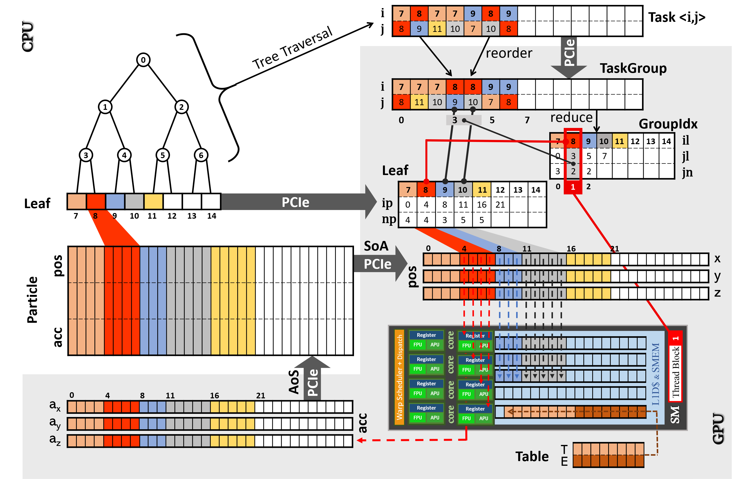
Figure 1: Memory layout and relation on CPU and GPU (shadow zone). The dark gray box denotes a SM unit. Arrows indicates the flow of data.

Fig 1 is schematic diagram of data arrays in the host memory and GPUs. There are three main data arrays for particle, leaf and tasks. Each particle structure contains position, velocity and acceleration, etc. We abstract the position information of x, y, z (Pos) into individual arrays (SoA) for further optimal GPU L2 cache performance. The task list (Task) of P2P interaction is an array of pair $<i,j>$ which indicates attractive force of particles in $i$-leaf induced by $j$-leaf.

They are sent to the GPU global memory denoted by the gray shadow zone. One Streaming Multiprocessor (SM) is shown with a dark gray box, which contains a chip of level-1 data cache (L1D$) plus shared memory (SMEM) and a group of sub-cores with registers and Float Point Units, etc. We allocate two main arrays to store Particle and Leaf. Each leaf records starting index of first particle and particle number in the leaf.

3.2 GPU kernel

Arrays of Task list, Leaf and Pos are transferred to the global memory of GPU via PCIe port. The item with the same index in Task list is not continuous in memory, which dramatically slows down the speed of data accesses into CUDA cores. To fix this problem, we reorder Task list with respect to $i$ and rename this list as TaskGroup. A CUDA library thrust is utilized for this reordering. Meanwhile the index array of Task Group (GroupIdx) is produced to record the starting points and length of tasks for every $i$-leaf in the task list.

According to the scheduling mechanism of GPU, we deal with all interactions in one task group with a thread block, which corresponds to a SM unit (Hamada et al. 2009). Since every task group contains only one $i$-leaf and all particles in $i$-leaf are continuously stored, each thread responds to one particle in $i$-leaf and the particles in $j$-leaf are prefetched into Shared memory for interaction calculation.

For instance, we assume that the gravity of leaf 8 is induced by leaf 9 and 10 in Fig. 1. As the 2nd column in ‘GroupIdx’, Thread block 1 is correspondent to it. Four particles in leaf 8 is sent into the register of sub-cores and particle position in leaf 9 and 10 are sent to shared memory of SM. Core function returns the acceleration acc$\_$i of leaf 8 (see implementation of Core function in Alg. 2). After all calculation of gravity is done, array of acceleration is transferred back to host memory.

Algorithm 1 P2P Kernel

__shared__ sh_pos_j

for $b\leftarrow$ blockIdx.x to $len$(GroupIdx)  do

     i$\_$leaf = GroupIdx.il[b]

     $t$ = threadIdx.x

     if $t$ $\textless$ Leaf[i_leaf].np then

         load pos[$t$ + Leaf[i$\_$leaf].ip] to register pos_i

         reset register acc_i with 0

     end if

     j_start = GroupIdx.jl[b]

     j_end = GroupIdx.jl[b] + GroupIdx.jn[b]

     for $j\leftarrow$ j_start to j_end  do

         j_leaf = TaskGroup.j[$j$]

         __syncthreads__

         if $t$ $\textless$ Leaf[j_leaf].np then

              preload pos[$t$+Leaf[j_leaf].ip]

                to SMEM sh_pos_j

         end if

         __syncthreads__

         nj = Leaf[j_leaf].np

         acc_i $+=$ Core(pos_i, sh_pos_j; nj)

         $\triangleright$ goto Algorithm 2

     end for

     accumulate register acc_i to global memory acc

     $b$ += gridDim.x

end for$\triangleright$ block level parallelism

3.3 Interpolation function

In previous section, we present the kernel and memory layout on GPU. In function of Core, two special functions are necessary in this kind of splitting method. Compared with the computation of pair-wise inverse-square gravity, they seriously decrease the efficiency of P2P kernel. The Gaussian shaped prefactor contains an exponential function (exp) and an error function (erf). Unlike function rsqrt estimated by an ‘intrinsic’ implementation, exp could consume about 5.5 times the operations of add/mul in fast math library on a NVidia GPU. We catch the effective number of floating-point operations (flops) by the tool of nvprof and find that erf needs to implicitly call functions of rcp, exp and several extra operations. This estimation is also consistent with the measurement of Arafa et al. (2019).

In order to speed up the evaluation of special functions, we combine those two functions into a table for the interpolation algorithm. The truncation function (Eq. 1) can be transformed to an integral form,

$$T(x\equiv\frac{r}{2r_{s}})=\frac{4}{\sqrt{\pi}}\int_{x}^{\infty}u^{2}e^{-u^{2}}du,$$

by using partial integration. Obviously, its Taylor’s series reads

$$T(x) =T_{i} :T_{[0]}$$ (2)

$$+x_{i}^{2}E_{i}\epsilon :T_{[1]}$$

$$-x_{i}(x_{i}^{2}-1)E_{i}\epsilon^{2} :T_{[2]}$$

$$+(\frac{2}{3}x_{i}^{4}-\frac{5}{3}x_{i}^{2}+\frac{1}{3})E_{i}\epsilon^{3} :T_{[3]}$$

$$-x_{i}(\frac{1}{3}x_{i}^{4}-\frac{3}{2}x_{i}^{2}+1)E_{i}\epsilon^{4} :T_{[4]}$$

$$+\mathcal{O}(\epsilon^{5}),$$

where $\epsilon=x-x_{i}$ , $E_{i}=-4{\exp}({-x_{i}^{2}})/{\sqrt{\pi}}$ and $T_{i}=\textrm{erfc}\left(x_{i}\right)-x_{i}E_{i}/2$ at the $i$-th gird of table in the range of [0,3]. In this case, we set grid number of $E_{i}$ and $T_{i}$ to 512, considering the suitable capacity of shared memory (light and heavy brown arrays in Fig. 1).

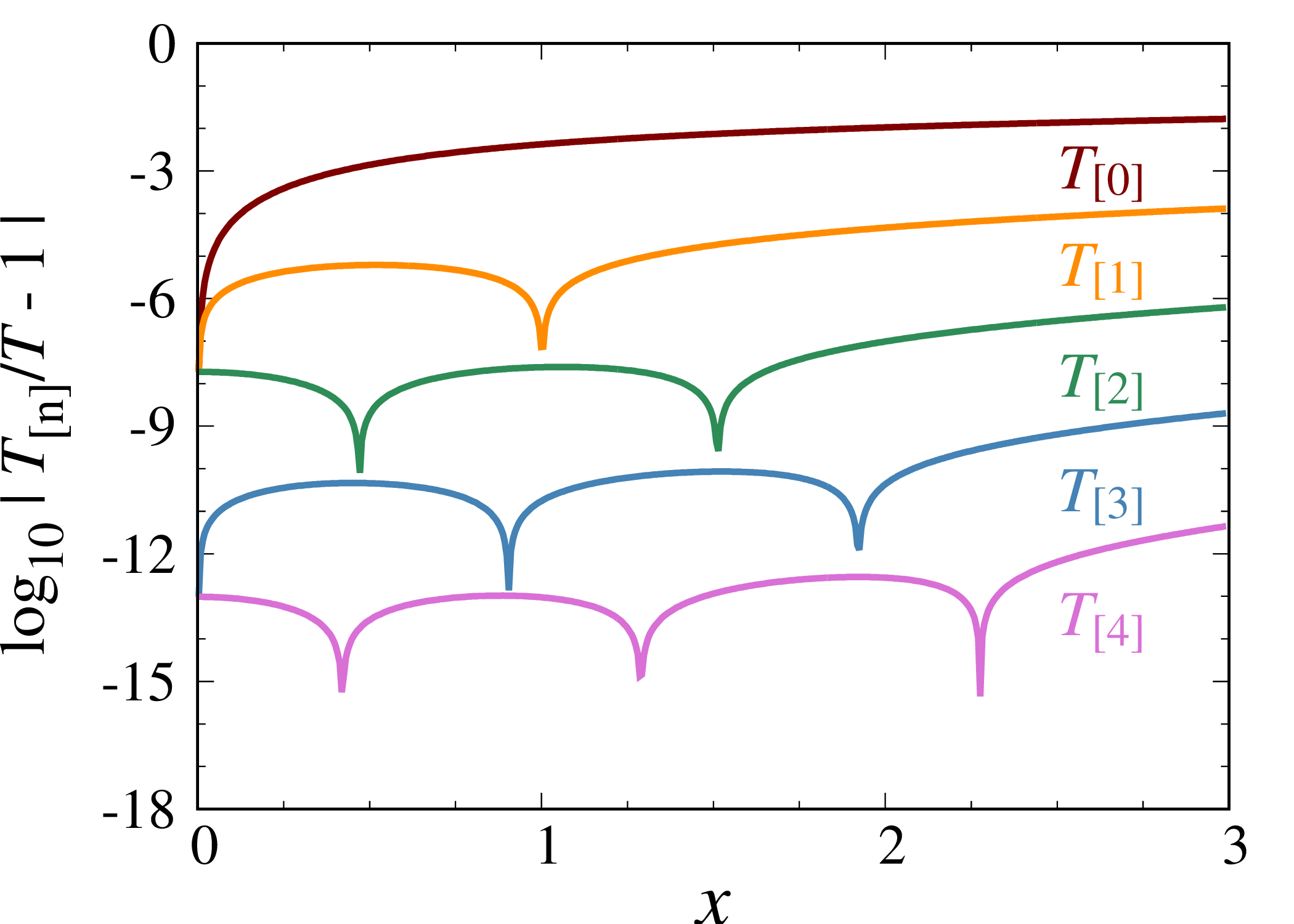
Figure 2: From top to bottom, The curves denote the maximum envelop of relative error with respect to exact splitting function at the interpolation level of $T_{[0]}$, $T_{[1]}$, $T_{[2]}$, $T_{[3]}$ and $T_{[4]}$, respectively.

We measure the precision of interpolation method to link accuracy with interpolation level. Fig. 2 shows that the maximum value of relative errors at different levels. We show the absolute value so that the transition of positive and negative value occurs at the position of the cusps of curves. According to the measurement result, $T_{[2]}$ is adequate for the single-precision calculation and $T_{[4]}$ is for double-precision. In the next section, we run some practical simulations to observe the overall interpolation effect.

Eq. 2 contains thirty nine floating point operations and $loads$ two float number from shared memory. The floating point operations can be reduced to fourteen by variable reuse and Fused Multiply-Add (FMA). Combining with other optimizations, the amount of flops can be suppressed by $\sim 60\%$ in total. The modified ‘Core’ is presented in Alg.  2.

Algorithm 2 Core function

function Core(pos_i, sh_pos_j; nj)

     for $j\leftarrow$ 0 to nj  do

         pos$\_$j = sh_pos_j[$j$] $\triangleright$ read from SMEM

         dx = pos$\_$j.x - pos$\_$i.x

         dy = pos$\_$j.y - pos$\_$i.y

         dz = pos$\_$j.z - pos$\_$i.z

         r2 = dx*dx + dy*dy + dz*dz

         determine table index $d$ and $\epsilon$ in Eq. 2

         load $T_{d}$

         load $E_{d}$

         idr = rsqrt(r2)

         pref   = $T_{[0]}(d,\epsilon)$

         pref += $T_{[1]}(d,\epsilon)$

         pref += $T_{[2]}(d,\epsilon)$ $\triangleright$ single precision

         pref += $T_{[3]}(d,\epsilon)$

         pref += $T_{[4]}(d,\epsilon)$ $\triangleright$ double precision

         grav = GM*idr*idr*idr*pref

         ax = grav*dx

         ay = grav*dy

         az = grav*dz

     end for

     return acc_i = (ax, ay, az)

end function$\triangleright$ thread level parallelism

4 test run

We modify the CPU-based PM-FMM code to a GPU-accelerated version that is referred to as PhotoNs-GPU. For testing the precision and efficiency of our code, we carry out two groups of cosmological simulations on a 1.5 TB memory GPU server with thirty-two cores of Intel Xeon 5218 CPU (2.3 GHz) and two NVidia Tesla 32GB V100S GPUs. The theoretic single precision (SP) performance of the machine is about 32.7 TFlops and the PCIe bandwidth is about 10 GB/s for each GPU.

4.1 Precision check

We test the accuracy of our code by comparing simulations run with Gadget-2 and PhotoNs-GPU. We employ $256^{3}$ particle in 1 $h^{-1}$Gpc simulation box. The initial condition at $z_{i}=99$ is generated by 2LPTic  (Crocce et al. 2006), which is evolved for four simulations by Gadget-2 and PhotoNs-GPU, respectively.

We use 16 MPI processes to carry out the simulation to the present $z=0$ with N${}_{\bf PM}=256$ and $100~{}h^{-1}$kpc softening length. Gadget-2 executes single step by 59 seconds of wall clock time and about 11,000 seconds in total. The power spectrum at $z=0$ is indicated with gray points in Fig. 3. Based on the same parameters and settings, we run two different simulations to check the influence of floating point precision on GPU. The calculation on GPU with single-precision (SP) is indicated with Golden dashed curve and double-precision (DP) is blue dash-dotted curve. In the same condition, PhotoNs-GPU executes single step by $\sim 1.3$ seconds of wall clock time and about 1,000 seconds in total, using 16 MPI processes and two V100 GPUs.

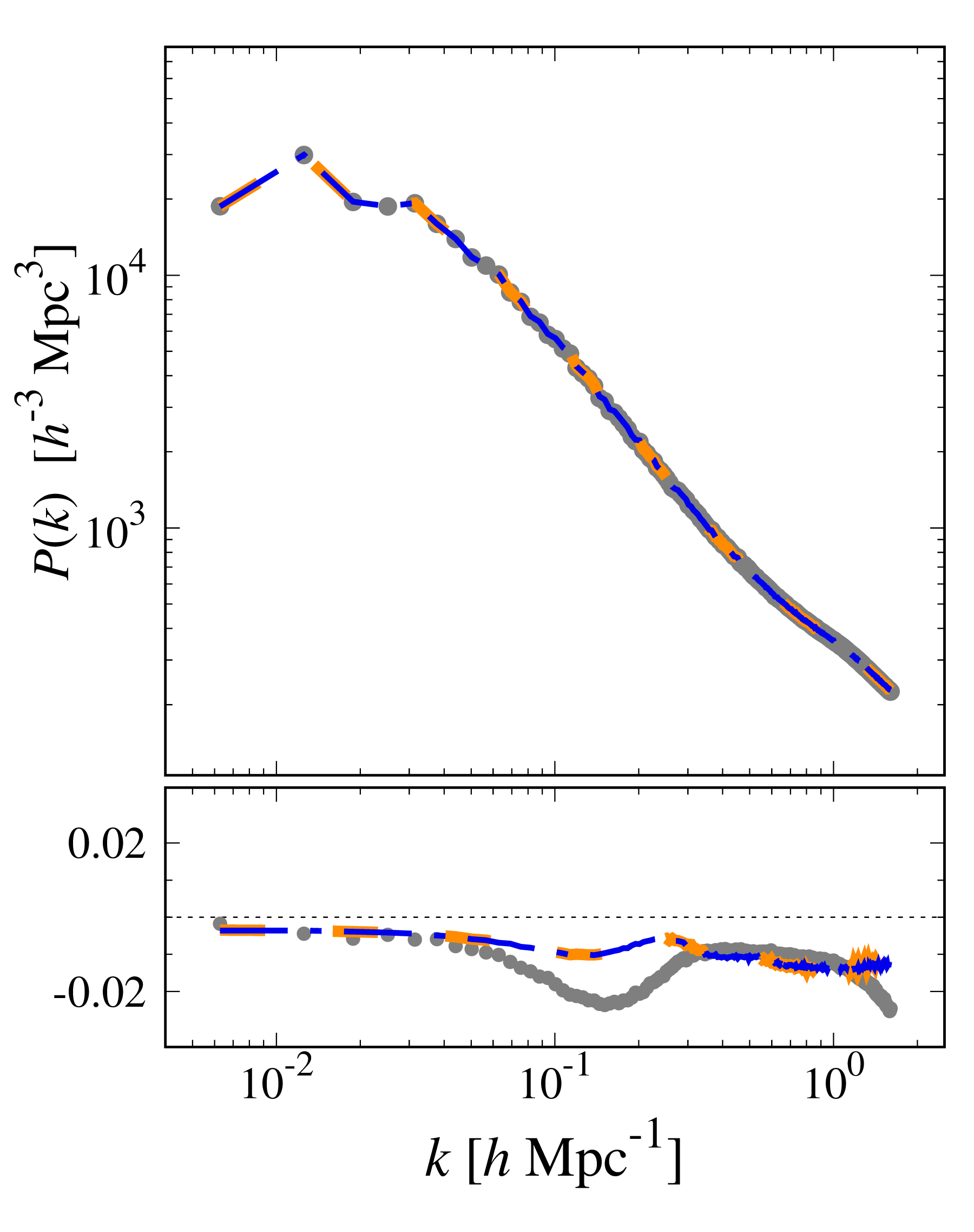
Figure 3: The comparison of power spectrum at z=0. The gray points denote Gadget-2 result, the heavy orange dashed line denotes SP run and the blue dash-dotted line denotes DP run by PhotoNs-GPU. In the bottom panel, the residuals of power spectrum show that the DP and SP runs are both consistent with the fiducial one.

The forth simulation is carried out as a fiducial one, which adopt direct P2P method to replace the Tree or FMM in order to exactly compute short-range gravity. Meanwhile we increase time steps by roughly three times. The bottom panel of Fig. 3 is the residual of power spectrum with respect to the fiducial simulation. The contrast of power spectrum is smaller than 1$\%$. Fig 3 shows that the SP case is well consistent with DP one, but more noisy at small scale ($k\sim 1$). Since PhotoNs-GPU employs a larger cutoff radius and more P2P contribution for gravity solver, our accuracy is slightly better than Gadget-2 in power spectrum statistics at the same settings.

4.2 Planck’s cosmology

According to the recent observation of the best-fit ’plik’ cosmological parameters from Planck 2018 (Planck Collaboration et al. 2020): $\Omega_{\mathrm{\Lambda}}$=0.684, $\Omega_{\mathrm{c}}$= 0.265, $\Omega_{\mathrm{b}}$ = 0.0494, $H_{0}$= 67.32 $km~{}s^{-1}$Mpc^-1, $\sigma_{8}$=0.812 and $n_{s}$ = 0.966, we employ $512^{3}$ particles in 100 $h^{-1}$Mpc simulation box. Since the test in the previous section indicates that a mixed-precision run is also consistent with the fiducial results in DP, we set all variable as SP to reduce the memory occupation and amount of communications and to utilize more Floating points units. The execution time is about five hours of wall clocks from redshift $z=99$ to $z=0$, using sixteen MPI processes and two Tesla V100S GPUs.

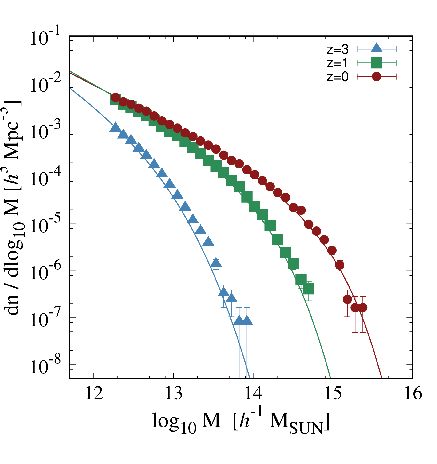
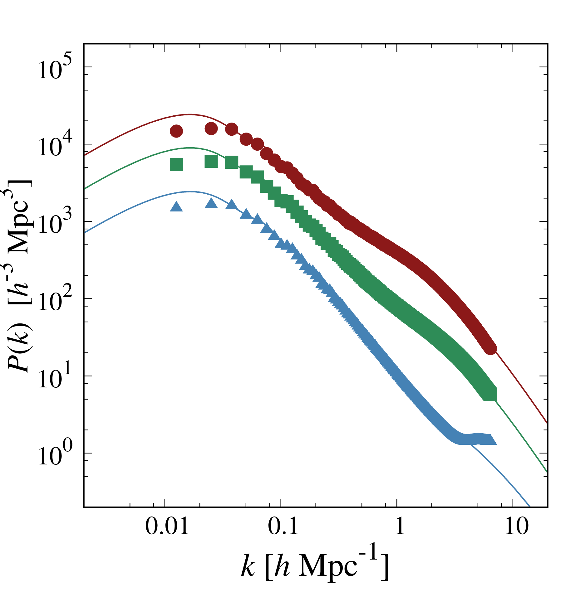
Figure 4: The comparison of mass function (left panel) and power spectrum (right panel) of test run with theoretical curves. The (red) points, (green) squares and (blue) triangles denote the simulation results at $z=0,1,3$, respectively.

The initial condition is constructed by a built-in IC module, following the Zel’dovich approximation method(Springel 2015) to effectively match our domain decomposition. The built-in module is based on the subroutine of 2LPTic and the notations are following the appendix A of Crocce et al. (2006). The input initial power spectrum is calculated by CAMB (Lewis et al. 2000).

Dark haloes mass functions at redshift $z=0,1,3$ are shown in the left panel of Fig. 4 and power spectra in the right panel. The mass function is measured by an on-the-fly Friend-of-Friend (FoF) halos finder and the theoretical curves are produced by Reed et al. (2007). The non-linear power spectrum is predicted by the HALOFIT (Takahashi et al. 2012; Mead et al. 2016). The deviation of power spectrum of $z=3$ (triangles) occurs at scale of $k\sim 5$. It could be due to the lack of sampling. Higher resolution test shows that that deviation disappears and the simulation result is well consistent with the predictions.

5 discussion

We present a GPU implementation of the PM-FMM algorithm by using an interpolated improvement for truncated pairwise interactions, then we tune the data structure to speed up GPU memory accesses and adjust the order of instructions in the kernel. A SP level test shows that SP runs can catch adequate accuracy on the statistics of large scale structure.

Briefly, after memory arrangement, interpolation and instruction fine tuning, the efficiency of code is significantly improved. In the case of the $512^{3}$ simulations with Planck’s cosmology , the number of particle-particle interactions per step averaged in the first ten steps is $\sim 1.74\times 10^{12}$. The mean wall-clock time per step is 7.62 seconds, in which the kernel time is 5.5 seconds. Thus, the average performance is 11.65 TFlops and the peak performance of the kernel is 16.134 TFlops. Here, we use the operation count of 51 per interaction. On our 32.7 TFlops server, the measured efficiency of averaged and peak performance reaches 35% and 48% on GPU, respectively.

Although the optimizations and tests in this work are carried out on a small server, PhotoNs-GPU is potentially powerful for massive parallelism on supercomputers. Therefore we add a built-in IC generator and an on-the-fly halo finder (Sun et al. 2020) into the code to save data storage. More on-the-fly data processes will be included into the code in the future.

We only focus on the P2P operator of the algorithm on GPUs in this work. We measure its performance and verify the feasibility for cosmological simulations. But there still needs more considerations and improvements on the other functional modules. For instance, M2L operator becomes more important for small box simulations or in isolated boundary conditions. Similarly, FFT in PM method could become dominant in extremely large simulations. Further optimizations and considerations about them will be done in our future works.