Voxel-Mesh Network for Geodesic-Aware 3D Semantic Segmentation of Indoor Scenes

Abstract

In recent years, sparse voxel-based methods have become the state-of-the-arts for 3D semantic segmentation of indoor scenes, thanks to the powerful 3D CNNs. Nevertheless, being oblivious to the underlying geometry, voxel-based methods suffer from ambiguous features on spatially close objects and struggle with handling complex and irregular geometries due to the lack of geodesic information. In view of this, we present Voxel-Mesh Network (VMNet), a novel 3D deep architecture that operates on the voxel and mesh representations leveraging both the Euclidean and geodesic information. Intuitively, the Euclidean information extracted from voxels can offer contextual cues representing interactions between nearby objects, while the geodesic information extracted from meshes can help separate objects that are spatially close but have disconnected surfaces. To incorporate such information from the two domains, we design an intra-domain attentive module for effective feature aggregation and an inter-domain attentive module for adaptive feature fusion. Experimental results validate the effectiveness of VMNet: specifically, on the challenging ScanNet dataset for large-scale segmentation of indoor scenes, it outperforms the state-of-the-art SparseConvNet and MinkowskiNet (74.6% vs 72.5% and 73.6% in mIoU) with a simpler network structure (17M vs 30M and 38M parameters).

1 Introduction

Thanks to the tremendous progress of RGB-D scanning methods in recent years [65, 27, 10], reliable tracking and reconstruction of 3D surfaces using hand-held, consumer-grade devices have become possible. Using these methods, large-scale 3D datasets with reconstructed surfaces and semantic annotations are now available [8, 4]. Nevertheless, compared to 3D surface reconstruction, 3D scene understanding, i.e., understanding the semantics of reconstructed scenes, is still a relatively open research problem.

Inspired by the success of 2D CNN in image semantic segmentation [5, 36], researchers have paid much attention to the straightforward extension of this idea to 3D, by performing volumetric convolution on regular grids [39, 68, 45]. Specifically, surface reconstructions are first projected to a discrete 3D grid representation, and then 3D convolutional filters are applied to extract features by sliding kernels over neighboring grid voxels [55, 64, 74]. Such features can be smoothly propagated in the Euclidean domain to accumulate strong contextual information. Unfortunately,

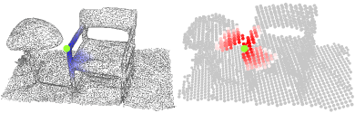
Figure 1: Illustration of geodesic information loss caused by voxelization. Considering the green point at the arm of a chair, on an input 3D mesh surface (Left), its geodesic neighbors (blue) can be easily collected, and the points of different objects are naturally separated. After voxelization (Right), geodesic information is discarded and only Euclidean neighbors (red) that are agnostic to the underlying surface can be extracted. The scan section is taken from the ScanNet dataset [8].

dense voxel-based methods require intensive computational power and are thus limited to low-resolution cases [35]. To process large-scale data, sparse voxel convolutions [17, 7] have been proposed to lower the computational requirement by ignoring inactive voxels. Benefiting from the efficient sparse voxel convolutions, complex networks have been built, achieving leading results on several 3D semantic segmentation benchmarks [8, 4] and outperforming other methods by large margins.

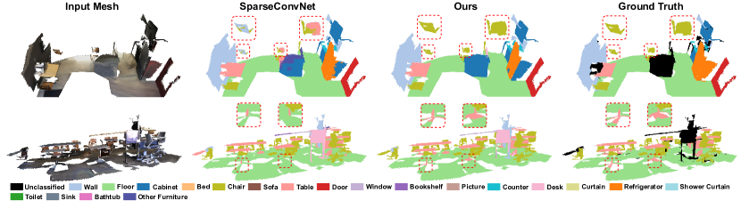
Figure 2: Limitations of voxel-based methods. (Upper) Some points of “chairs” are mistakenly classified into nearby classes in the Euclidean space by SparseConvNet [17] since the convolutional filters produce ambiguous features for spatially close objects. (Lower) On areas with complex and irregular geometries (e.g. , the base parts of “tables”), SparseConvNet fails to predict correct results due to the lack of geodesic information about shape surfaces.

Despite the remarkable achievements, voxel-based methods are not perfect. One of their major limitations is the geodesic information loss caused by the voxelization process (see Fig. 1). Recent public datasets like ScanNet [8] provide 3D scene reconstructions in the form of high-quality triangular meshes, in which the surface information is naturally encoded. On these meshes, vertices belonging to different objects are well separated, and geodesic features can be easily aggregated through edge connectivities. However, the voxelization process omits all mesh edges and only retains Euclidean positions of mesh vertices. Consequently, convolutional filters operating on voxels are agnostic to the underlying surfaces and, therefore, result in two problems. First, these filters generate similar features for voxels that are close in the Euclidean domain, even though these voxels may belong to different objects and are distant in the geodesic domain. As shown in the top example of Fig. 2, these ambiguous features produce sub-optimal predictions for objects that are spatially close. Second, without the geodesic information about shape surfaces, these Euclidean convolutions may struggle with learning specific object shapes. As shown in the lower example of Fig. 2, this property is problematic for segmentation on areas with complex and irregular geometries.

We have discussed the advantages of voxel-based methods on contextual learning and their problems on geodesic information loss. It is appealing to design a method resolving the problems while retaining these advantages by leveraging both the Euclidean and geodesic information. A possible solution is to take voxels and the original meshes as the sources for the Euclidean and geodesic information, respectively. It is therefore natural to ask how these two representations can be combined in a common architecture.

To address this question, we propose the Voxel-Mesh network (VMNet), a novel deep hierarchical architecture for geodesic-aware 3D semantic segmentation. Starting from a mesh representation, to extract informative contextual features in the Euclidean domain, we first voxelize the input mesh and apply sparse voxel convolutions. Next, to incorporate the geodesic information, the extracted contextual features are projected from the Euclidean domain to the geodesic domain, specifically, from voxels to mesh vertices. These projected features are further fused and aggregated to combine both the Euclidean and geodesic information.

In order to build such a deep architecture that is capable of effectively learning useful features incorporating information from the two domains, it is critical to design proper ways to aggregate intra-domain features and to fuse inter-domain features. In view of the great success of self-attention operators for feature processing [60, 42, 34], we therefore present two key components of VMNet: Intra-domain Attentive Aggregation Module and Inter-domain Attentive Fusion Module. The former aims to aggregate the projected features on the original meshes to incorporate the geodesic information and the latter focuses on the effective fusion of features from the two domains.

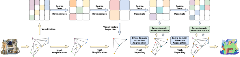
Figure 3: Overview of Voxel-Mesh Network (VMNet). Taking a colored mesh as input, we first rasterize it and apply voxel-based sparse convolutions to extract contextual information in the Euclidean domain. These features are then projected from voxels to vertices, and are further aggregated and fused in the geodesic domain producing distinctive per-vertex features. For simplicity, skip connections between the encoder and decoder are neglected here and only three levels of hierarchical voxel downsampling and mesh simplification are shown.

We conduct extensive experiments to demonstrate the effectiveness of our method on the popular ScanNet v2 benchmark [8] and the recent Matterport3D benchmark [4]. VMNet outperforms existing sparse voxel-based methods SparseConvNet [17] and MinkowskiNet [7] (74.6% vs 72.5% and 73.6% in mIoU) with a simpler network structure (17M vs 30M and 38M parameters) on the ScanNet dataset and sets a new state-of-the-art on the Matterport3D dataset.

To summarize, our contributions are threefold:

1. We propose a novel deep architecture, VMNet, which operates on the voxel and mesh representations, leveraging both the Euclidean and geodesic information.

2. We propose an intra-domain attentive aggregation module, which effectively refines geodesic features through edge connectivities.

3. We propose an inter-domain attentive fusion module, which adaptively combines Euclidean and geodesic features.

2 Related Work

In this section, we first review relevant works on 3D semantic segmentation, organized according to their inherent convolutional categories, and then discuss the application of attention mechanism in 3D semantic segmentation.

2D-3D. A conventional way of performing 3D semantic segmentation is to first represent 3D shapes through their 2D projections from various viewpoints, and then leverage existing image segmentation techniques and architectures from the 2D domain [30, 29]. Instead of choosing a global projection viewpoint, some researchers have proposed to project local neighborhoods to local tangent planes and process them with 2D convolutions [58, 70, 23]. Taking the RGB frames as additional inputs, other researchers have proposed methods that combine 2D and 3D features through 2D-3D projection [9, 20]. Although these methods can easily benefit from the success of image segmentation techniques (mainly based on 2D CNNs), they often require a large amount of additional 2D data, involve a complex multi-view projection process, and rely heavily on viewpoint selection. Some of these methods have attempted to utilize geodesic information implicitly through mesh textures [23] or point normal [58]. They achieve fairly decent results but fail to fully exploit the geodesic information.

PointConv & SparseConv. Partly due to the difficulties of handling mesh edges in deep neural networks, most existing 3D semantic segmentation methods take raw point clouds or transformed voxels as input [3, 30, 51, 1, 48, 44, 46, 41, 62]. Point-based methods apply convolutional kernels to the local neighborhoods of points obtained using k-NN or spherical search [72, 63, 61, 56, 22, 67, 21]. Numerous designs of point-based convolutional kernels have been proposed [31, 28, 59, 37, 71]. In the case of voxel-based methods, the raw 3D data is first transformed into a voxel representation and then processed by standard CNNs [39, 45, 64, 74, 24]. To address the cubic memory and computation consumption problem of voxel-based operations, recent works have made efforts to propose efficient sparse voxel convolutions [17, 7, 57]. In both point-based and voxel-based methods, features are aggregated over the Euclidean space only. In contrast, we additionally consider geodesic information of the underlying object surfaces.

GraphConv. Graph convolution networks can be grouped into spectral networks [12, 54] and local filtering networks [38, 2, 40]. Spectral networks work well on clean synthetic data, but are sensitive to reconstruction noise and are thus not applicable to 3D semantic segmentation. Local filtering networks define handcrafted coordinate systems and apply convolutional operations over patches. For 3D semantic segmentation, these methods often perform over local neighborhoods of point clouds [26, 32] and are thus oblivious to the underlying geometry.

Our method falls into both the SparseConv and GraphConv categories. It is similar in spirit to the recent work of Schult et al. [52], which combines a Euclidean-based and a geodesic-based graph convolutions. However, instead of concatenating features obtained from different convolutional filters as done in [52], we first accumulate strong contextual information in the Euclidean domain and then adaptively fuse and aggregate geometric information in the geodesic domain, leading to a significant better segmentation performance (see Section 4.3).

Attention. For 3D semantic segmentation, most existing methods implement attention layers operating on the local neighborhoods of point clouds for feature aggregation [15, 61] or on downsampled point sets for context augmentation [69, 66]. In our work, instead of operating on point clouds, we build attentive operators applying on triangular meshes. Moreover, in contrast to previous works that process features in a single domain, we propose both an intra-domain module and an inter-domain module.

3 METHODOLOGY

In this section, we first give an overview of our voxel-mesh network in Section 3.1. Then we introduce the network architecture in Section 3.2. The voxel-based contextual feature aggregation branch is described in Section 3.3. Sections 3.4 and 3.5 depict the proposed attentive modules for intra-domain feature aggregation and inter-domain feature fusion, respectively. Finally, we discuss two well-known mesh simplification methods, which are used to build a mesh hierarchy for multi-level feature learning in Section 3.6.

3.1 Overview

VMNet deals with two types of 3D representations: voxels and meshes. As depicted in Fig. 3, the network consists of two branches: according to their operating domains, we denote the upper one as the Euclidean branch and the lower one as the geodesic branch.

To accumulate contextual information in the Euclidean domain, taking a mesh as input, the colored vertices are first voxelized and then fed to the Euclidean branch. Building on sparse voxel-based convolutions, we construct a U-Net [49] like encoder-decoder structure, where the encoder is symmetric to the decoder, including skip connections between both. Multi-level sparse voxel-based feature maps $(\mathcal{S}^{0},...,\mathcal{S}^{l},...,\mathcal{S}^{L})$ can be extracted from the decoder.

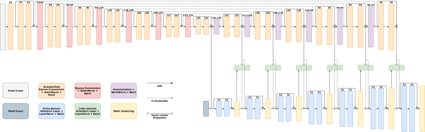
Figure 4: Network architecture of VMNet. We use a voxel-based 3D U-Net [49] as the contextual feature extractor, consisting of an encoder and a decoder. Afterwards, at each level of the decoder, the aggregated contextual features are first projected from the Euclidean domain to the geodesic domain, and then processed by the intra-domain attentive aggregation modules and the inter-domain attentive fusion modules defined over triangular meshes, yielding distinctive per-vertex features enriched with both the Euclidean and geodesic information. The number above each layer indicates the number of its corresponding feature channel.

Figure 5: 2D illustration of voxel-vertex projection. Vertices $(x_{1},y_{1})$ and $(x_{2},y_{2})$ share the same set of neighboring voxels but their projected features are different through trilinear interpolation (bilinear interpolation for the 2D case).

Although these contextual features offer valuable semantic cues for scene understanding, their unawareness of the underlying geometric surfaces will lead to sub-optimal results. Therefore, to incorporate geodesic information, the accumulated contextual features are projected from the Euclidean domain to the geodesic domain for further processing (Section 3.3). In the geodesic branch, we prepare a hierarchy of simplified meshes $(\mathcal{M}^{0},...,\mathcal{M}^{l},...,\mathcal{M}^{L})$, in which each level of simplified mesh $\mathcal{M}^{l}$ corresponds to a downsampling level of sparse voxels $\mathcal{S}^{l}$. Trace maps of the mesh simplification processes are saved for unpooling operations between mesh levels. At the first level of the decoding process (level $L$), the features are projected from voxels $\mathcal{S}^{L}$ to mesh vertices $\mathcal{M}^{L}$ and then refined through intra-domain attentive aggregation (Section 3.4). The resulting geodesic features of $\mathcal{M}^{L}$ are unpooled to the next level $\mathcal{M}^{L-1}$. At each following level $l$, the Euclidean features projected from $\mathcal{S}^{l}$ and the unpooled geodesic features of $\mathcal{M}^{l}$ are first adaptively combined through inter-domain attentive fusion (Section 3.5) and then the fused features are further refined through intra-domain attentive aggregation before being unpooled to the next level.

3.2 Network Architecture

The network architecture adopted in VMNet is illustrated in Fig. 4. In the upper branch (i.e., the Euclidean branch), the network is mainly built upon submanifold sparse convolution (SSC) layers and sparse convolution (SC) layers, both of which are originally introduced by Graham et al. [17] for 3D semantic segmentation. The basic building module is a residual block consisting of two layers of SSC with a skip connection implemented by addition. Each pair of adjacent residual blocks are connected through an SC layer, which performs downsampling (encoding stage) or upsampling (decoding stage) of the sparse voxels $\mathcal{S}$. In total, there are 13 residual blocks and 7 levels of sparse voxels $(\mathcal{S}^{0},...,\mathcal{S}^{l},...,\mathcal{S}^{6})$. In the lower branch (i.e., the geodesic branch), similar to the upper one, the network is constructed by residual blocks, each consisting of two layers of our proposed intra-domain attention layers (Section 3.4), which operate on the triangular meshes $\mathcal{M}$. Each pair of adjacent residual blocks in the geodesic branch are connected through a mesh unpooling layer. The distinctive per-vertex features on the last mesh level $\mathcal{M}^{0}$ are used for semantic prediction. Between the two branches, the projected Euclidean features and the aggregated geodesic features are adaptively fused through our proposed inter-domain attention layers (Section 3.5).

3.3 Voxel-based Contextual Feature Aggregation

Voxelization. At mesh level $\mathcal{M}^{0}$, with all edge connectivities omitted, the input features (colors) of mesh vertices $\{(V_{i},f_{i})\}$ are transformed into the voxel cells $\{V_{u,v,w}\}$ by averaging all features $f_{i}$ whose corresponding coordinate $V_{i}:(x_{i},y_{i},z_{i})$ falls into the voxel cell $(u,v,w)$:

$$\begin{split}f_{u,v,w}=\frac{1}{N_{u,v,w}}\sum_{i=1}^{n}B[floor(x_{i}\cdot r)=u,\\ floor(y_{i}\cdot r)=v,floor(z_{i}\cdot r)=w]\cdot f_{i},\end{split}$$ (1)

where $r$ denotes the voxel resolution, $B[\cdot]$ is the binary indicator of whether vertex $V_{i}$ belongs to the voxel cell $(u,v,w)$, and $N_{u,v,w}$ is the number of vertices falling into that cell [35].

Contextual Feature Aggregation. To accumulate contextual information, we construct a simple U-Net [49] structure based on voxel convolutions. We adopt the sparse implementation provided by [57].

Voxel-vertex Projection. With the contextual features aggregated in the Euclidean domain, at each level $l$, we transform the features of voxels $\mathcal{S}^{l}$ back to vertices $\mathcal{M}^{l}$ for further processing in the geodesic domain. Inspired by previous works [35, 57], we compute each vertex’s feature utilizing trilinear interpolation over its neighboring eight voxels. Through this means, the projected features are distinct even for the vertices sharing the same set of neighboring voxels. A 2D illustration of the projection is shown in Fig. 5.

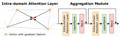
Figure 6: Illustration of intra-domain attentive aggregation module. (Left) Intra-domain attention layer operates on mesh vertices aggregating geodesic information through edge connectivities. (Right) The aggregation module consists of two attention layers with skip connections.

3.4 Intra-domain Attentive Aggregation Module

After contextual feature aggregation and voxel-vertex projection, to effectively refine the projected features, we design an intra-domain attentive aggregation module operating on the geodesic domain. As shown in Fig. 6 (Left), at each mesh level, we perform attentive aggregation on the graph $\mathcal{G}=(\mathcal{V},E)$ induced by the underlying mesh $\mathcal{M}$. Note that we neglect the level superscript $l$ to ease readability. Our intra-domain attention layer is based on the standard scalar attention [60], which is often used for point clouds in 3D semantic segmentation, but not for triangular meshes. Specifically, at layer $k$, the output feature $f_{i}^{{}^{\prime}geo}$ of vertex $V_{i}$ with an input feature $f_{i}^{geo}$ is computed as:

$$\begin{split}f_{i}^{{}^{\prime}geo}=\rho^{intra}_{k}(f_{i}^{geo})+\sum_{j\in N_{i}}\omega_{ij}\alpha^{intra}_{k}(f_{j}^{geo}),\\ \omega_{ij}=softmax(\frac{\varphi^{intra}_{k}(f_{i}^{geo})^{T}\psi^{intra}_{k}(f_{j}^{geo})}{\sqrt{d}}),\end{split}$$ (2)

where $N_{i}$ is the one-ring neighborhood of vertex $V_{i}$. The functions $\rho^{intra}_{k}$, $\alpha^{intra}_{k}$, $\varphi^{intra}_{k}$, and $\psi^{intra}_{k}$ are vertex-wise feature transformations implemented by MLP, $\omega_{ij}$ is the attention coefficient, and $d$ is the size of output feature channels. Since the positional information is naturally embedded in the voxel-based contextual feature aggregation step, we do not implement a position encoding function explicitly. Our attention layer is inspired by the implementation in [53], which operates on abstract graphs for semi-supervised node classification, while our method operates on 3D mesh graphs for geodesic feature aggregation.

Building on the intra-domain attention layer, we design an aggregation module performing two steps of attentive feature aggregation on each simplified mesh level (see Fig. 6 (Right)).

3.5 Inter-domain Attentive Fusion Module

Operating on both the voxel and mesh representations poses a demand for Euclidean and geodesic feature fusion. To adaptively combine features from the two domains, we propose an inter-domain attentive fusion module. As depicted in Fig. 7 (Left), between each pair of sparse voxel level $\mathcal{S}$ and mesh level $\mathcal{M}$ (except for level $L$), we perform attentive fusion on the same graph $\mathcal{G}=(\mathcal{V},E)$ as the one used for intra-domain aggregation (level superscript $l$ is neglected).

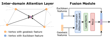
Figure 7: Illustration of inter-domain attentive fusion module. (Left) Inter-domain attention layer adaptively combines geodesic features and Euclidean features on mesh vertices. (Right) The fused feature map generated by the inter-domain attention layer is further combined with the original geodesic feature map and the projected Euclidean feature map through concatenation.

However, unlike intra-domain attention, which processes features in the same domain, inter-domain attention takes as input both the geodesic features $f^{geo}$ and the Euclidean features $f^{euc}$ projected from voxels. At layer $k$, the fused feature $f_{i}^{fuse}$ of vertex $V_{i}$ is computed as:

$$\begin{split}f_{i}^{fuse}=\rho^{inter}_{k}(f_{i}^{euc})+\sum_{j\in N_{i}}\omega_{ij}\alpha^{inter}_{k}(f_{j}^{geo}),\\ \omega_{ij}=softmax(\frac{\varphi^{inter}_{k}(f_{i}^{euc})^{T}\psi^{inter}_{k}(f_{j}^{geo})}{\sqrt{d}}),\end{split}$$ (3)

where $N_{i}$ is the same one-ring neighborhood of vertex $V_{i}$ as the one used for intra-domain aggregation. Unlike the one in intra-domain attention, the inter-domain attention coefficient $\omega_{ij}$ is conditioned on both the Euclidean and geodesic features enabling the network to adaptively fuse features from the two domains.

As shown in Fig. 7 (Right), the proposed inter-domain attentive fusion module takes both the Euclidean features and the geodesic features as inputs. These features are fed to one inter-domain attention layer followed by layer normalization and ReLU activation. Before being passed on for further processing, the fused feature map is concatenated with the projected Euclidean feature map and the original geodesic feature map.

3.6 Mesh Simplification

To construct a deep architecture for multi-level feature learning, we generate a hierarchy of mesh levels $(\mathcal{M}^{0},...,\mathcal{M}^{l},...,\mathcal{M}^{L})$ of increasing simplicity, interlinked by pooling trace maps. Each level of simplified mesh corresponds to a level of downsampled 3D sparse voxels. For mesh simplification, there are two well-known methods from the geometry processing domain: Vertex Clustering (VC) [50] and Quadric Error Metrics (QEM) [16]. As shown in Fig. 8, during the vertex clustering process, a 3D uniform grid with cubical cells of a fixed side length is placed over the input graph and all vertices falling into the same cell are grouped. This generates uniform-sampled simplified meshes, possibly with topology changes and non-manifold faces. On the contrary, the QEM method incrementally collapses mesh edges according to an approximate error of the geometric distortion introduced by this collapse, and thus has explicit control over mesh topology (see Fig. 9). Since our goal is to extract meaningful geodesic information, we prefer the QEM method for its better topology-preserving property.

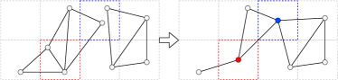
Figure 8: Illustration of Vertex Clustering for mesh simplification. Vertices falling in the same cell are merged to form a new vertex. The resulting mesh might be non-manifold (red cell) or have its topology changed (blue cell).

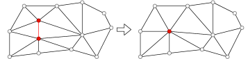
Figure 9: Illustration of Quadric Error Metrics based edge collapse for mesh simplification. The edge between two red vertices is collapsed and the resulting mesh is re-triangulated with its topology preserved.

However, directly applying the QEM method on the original meshes results in high-frequency signals in noisy areas [52]. Therefore, we apply the VC method on the original mesh for the first two mesh levels and then apply the QEM method for the remaining mesh levels. We present an ablation study on mesh simplification methods in Section 4.4.

4 EXPERIMENTS

To demonstrate the effectiveness of our proposed method, we now present various experiments conducted on two large-scale 3D scene segmentation datasets, which contain meshed point clouds of various indoor scenes. We first introduce the datasets and evaluation metrics that we used in Section 4.1, and then present the implementation details for reproduction in Section 4.2. We report the results on the ScanNet and Matterport3D datasets in Section 4.3, and the ablation studies in Section 4.4.

4.1 Datasets and Metrics

ScanNet v2 [8]. ScanNet dataset contains 3D meshed point clouds of a wide variety of indoor scenes. Each scene is provided with semantic annotations and reconstructed surfaces represented by a textured mesh. The dataset contains 20 valid semantic classes. We perform all our experiments using the public training, validation, and test split of 1201, 312, and 100 scans, respectively.

Matterport3D [4]. Matterport3D is a large RGB-D dataset of 90 building-scale scenes. Similar to ScanNet, the full 3D mesh reconstruction of each building and semantic annotations are provided. The dataset contains 21 valid semantic classes. Following previous works [52, 46, 56, 58, 9, 23], we split the whole dataset into training, validation, and test sets of size 61, 11, and 18, respectively.

Metrics. For evaluation, we use the same protocol as introduced in previous works [52, 46, 7, 17]. We report mean class intersection over union (mIoU) results for ScanNet and mean class accuracy for Matterport3D. During testing, we project the semantic labels to the vertices of the original meshes and test directly on meshes.

TABLE I: Mean intersection over union scores on ScanNet Test [8]. Detailed results can be found on the ScanNet benchmarking websiteand in the supplementary material.

Method	mIoU(%)	Conv Category
TangentConv [58]	43.8	2D-3D
SurfaceConvPF [70]	44.2
3DMV [9]	48.3
TextureNet [23]	56.6
JPBNet [6]	63.4
MVPNet [25]	64.1
V-MVFusion [29]	74.6
BPNet [20]	74.9
PointNet++ [46]	33.9	PointConv
FCPN [47]	44.7
PointCNN [33]	45.8
DPC [13]	59.2
MCCN [19]	63.3
PointConv [67]	66.6
KPConv [59]	68.4
JSENet [21]	69.9
SparseConvNet [17]	72.5	SparseConv
MinkowskiNet [7]	73.6
SPH3D-GCN [32]	61.0	GraphConv
HPEIN [26]	61.8
DCM-Net [52]	65.8
VMNet (Ours)	74.6	Sparse+Graph Conv

4.2 Implementation Details

In this section, we discuss the implementation details for our experiments. VMNet is coded in Python and PyTorch (Geometric) [14, 43]. All the experiments are conducted on one NVIDIA Tesla V100 GPU.

Data Preparation. We perform training and inference on full meshes without cropping. For the Euclidean branch of VMNet, input meshes are voxelized at a resolution of 2 cm. To compute the hierarchical mesh levels accordingly for the geodesic branch, we first apply the VC method on the input mesh with the respective cubical cell lengths of 2 cm and 4 cm for the first two mesh levels. For each remaining level, the QEM method is applied to simplify the mesh until the vertex number is reduced to 30% of its preceding mesh level. For better generalization ability, edges of all mesh levels are randomly sampled during training. We use the vertex colors as the only input features and apply data augmentation, including random scaling, rotation around the gravity axis, spatial translation, and chromatic jitter.

Training Details. We train the network end-to-end by minimizing the cross entropy loss using Momentum SGD with the Poly scheduler decaying from learning rate 1e-1.

TABLE II: Mean class accuracy scores on the Matterport3D Test [4]. The same network definition as for the ScanNet benchmark is used. Conv Category: (I) 2D-3D, (II) PointConv, (III) VoxelConv, (IV) GraphConv, (V) Sparse+Graph Conv.

Method	mAcc(%)	Cat	wall	floor	cab	bed	chair	sofa	table	door	wind	shf	pic	cntr	desk	curt	ceil	fridg	show	toil	sink	bath	other
TangentConv [58]	46.8	I	56.0	87.7	41.5	73.6	60.7	69.3	38.1	55.0	30.7	33.9	50.6	38.5	19.7	48.0	45.1	22.6	35.9	50.7	49.3	56.4	16.6
3DMV [9]	56.1	I	79.6	95.5	59.7	82.3	70.5	73.3	48.5	64.3	55.7	8.3	55.4	34.8	2.4	80.1	94.8	4.7	54.0	71.1	47.5	76.7	19.9
TextureNet [23]	63.0	I	63.6	91.3	47.6	82.4	66.5	64.5	45.5	69.4	60.9	30.5	77.0	42.3	44.3	75.2	92.3	49.1	66.0	80.1	60.6	86.4	27.5
SplatNet [56]	26.7	II	90.8	95.7	30.3	19.9	77.6	36.9	19.8	33.6	15.8	15.7	0.0	0.0	0.0	12.3	75.7	0.0	0.0	10.6	4.1	20.3	1.7
PointNet++ [46]	43.8	II	80.1	81.3	34.1	71.8	59.7	63.5	58.1	49.6	28.7	1.1	34.3	10.1	0.0	68.8	79.3	0.0	29.0	70.4	29.4	62.1	8.5
ScanComplete [11]	44.9	III	79.0	95.9	31.9	70.4	68.7	41.4	35.1	32.0	37.5	17.5	27.0	37.2	11.8	50.4	97.6	0.1	15.7	74.9	44.4	53.5	21.8
DCM-Net [52]	66.2	IV	78.4	93.6	64.5	89.5	70.0	85.3	46.1	81.3	63.4	43.7	73.2	39.9	47.9	60.3	89.3	65.8	43.7	86.0	49.6	87.5	31.1
VMNet (Ours)	67.2	V	85.9	94.4	56.2	89.5	83.7	70.0	54.0	76.7	63.2	44.6	72.1	29.1	38.4	79.7	94.5	47.6	80.1	85.0	49.2	88.0	29.0

TABLE III: Comparison of run-time complexity against SOTA sparse voxel-based methods. For a fair comparison, we report the latencies of both their original versions (Ori) and our implementations using the same type of sparse convolution (TS) as VMNet.

Method	Params (M)	Latency (ms)		mIoU(%)
		Ori	TS
SparseConvNet [17]	30.1	712	102	72.5
MinkowskiNet [7]	37.8	629	105	73.6
VMNet (Ours)	17.5	-	107	74.6

TABLE IV: Comparison of run-time complexity against SOTA methods of different convolutional categories.

Method	Conv Category	Params (M)	Latency (ms)	mIoU(%)
MVPNet[25]	2D-3D	24.6	95	64.1
PointConv[67]	PointConv	21.7	307	66.6
KPConv[59]	PointConv	14.1	52	68.4
DCM-Net[52]	GraphConv	0.76	151	65.8
VMNet (Ours)	Sparse+Graph Conv	17.5	107	74.6

4.3 Results and Analysis

Quantitative Results. We present the performance of our approach compared to recent competing approaches on the ScanNet benchmark [8] in Table 1. All the methods are grouped by the approaches’ inherent convolutional categories as discussed in Section 2. As shown in Table 1, our method leads to a 74.6% mIoU score, achieving a significant performance gain of 8.8 % mIoU comparing to the existing best-performing graph convolutional approach, i.e., DCM-Net [52], and 1.0 % mIoU comparing to the leading sparse convolutional approach, i.e., MinkowskiNet [7]. Our method achieves results comparable to the SOTA 2D-3D method BPNet [20], which is a concurrent work on CVPR2021 utilizing both 2D and 3D data while VMNet takes as input only the 3D data. For a fair comparison, the result of OccuSeg [18] is not listed in this table, since it utilizes extra instance labels for training. We also evaluate our algorithm on the novel Matterport3D dataset [4] and report the results in Table II. VMNet achieves overall state-of-the-art results outperforming the previous best method by 1% in terms of mean class accuracy. Since some methods only report results in one of these two datasets, the listed methods in Tables 1 and II are different.

Qualitative Comparison. Fig. 10 shows our qualitative results on the ScanNet validation set and Fig. 11 shows the results on the Matterport3D test set. Compared to the SOTA sparse voxel-based method SparseConvNet, which operates in the Euclidean domain solely, VMNet generates more distinctive features for close-located objects and better handles complex geometries thanks to the combined Euclidean and geodesic information. More qualitative results can be found in the supplementary material.

Complexity. We compare our method with representative SOTA methods of various convolutional categories in terms of their run-time complexity. We randomly select a scene from the ScanNet validation set and compute the latency results by averaging the inference time of 100 forward passes.

TABLE V: Ablation study: (Left) Euclidean and geodesic information; (Right) Network components.

Information	mIoU(%)
Geo Only	58.1
Euc Only	71.0
VMNet(Geo+Euc)	73.3

Baseline	Intra	Inter	mIoU(%)
✓			70.2
✓	✓		72.1
✓	✓	✓	73.3

TABLE VI: Ablation study: (Left) Attentive operators; (Right) Mesh simplification.

Operator	mIoU(%)
Vector Attention	72.3
EdgeConv	72.6
Scalar Attention	73.3

Method	mIoU(%)
VC only	72.3
QEM only	72.9
VC + QEM	73.3

In Table III, we present the results of two SOTA sparse voxel-based methods, i.e., SparseConvNet [17] and MinkowskiNet [7]. Although the accuracies of sparse voxel-based methods are not dependent on the implementation of sparse convolution, the latencies of these methods are highly dependent on the implementation. Therefore, we re-implement SparseConvNet and MinkowskiNet using the same version of sparse convolution (i.e., torchsparse [57]) as VMNet for a fair comparison. As shown in the table, VMNet achieves the highest mIoU score with the least number of parameters. It implies that, compared to extracting features in the Euclidean domain alone, combining the Euclidean and geodesic information leads to a more effective aggregation of features, even with a simpler network structure. The latency of VMNet is slightly higher than our new implementations of the other two methods. This is caused by the unoptimized projection operations, which are left for future improvement.

In Table IV, we report more complexity comparisons of our network against other representative methods, including MVPNet[25], PointConv[67], KPConv[59], and DCM-Net[52]. While achieving the highest mIoU, VMNet is largely comparable to these representative methods, in terms of both inference time and parameter size.

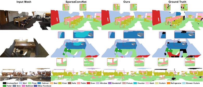
Figure 10: Qualitative results on ScanNet Val [8]. The key parts for comparison are highlighted by dotted red boxes.

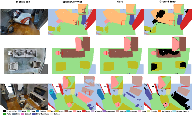
Figure 11: Qualitative results on Matterport3D Test [4]. The key parts for comparison are highlighted by dotted red boxes.

4.4 Ablation Study

In this section, we conduct a number of controlled experiments that demonstrate the effectiveness of building modules in VMNet, and also examine some specific decisions in VMNet design. Since the test set of ScanNet is not available for multiple tests, all experiments are conducted on the validation set, keeping all hyper-parameters the same.

Euclidean and Geodesic Information. In Section 3, we advocate the combination of Euclidean and geodesic information. To investigate their impacts, we compare VMNet to two baseline networks: “Euc only” is a U-Net structure based on sparse convolutions operating on voxels and “Geo only” has the same structure but is based on the proposed intra-domain attention layers operating on meshes. For a fair comparison, we keep the layer numbers of these baselines the same as the Euclidean branch of VMNet but increase their channel numbers to make sure all the compared methods have similar parameter sizes. As shown in Table V (Left), VMNet outperforms the two baselines showcasing the benefit of combining information from the two domains.

Network Components. In Table V (Right), we evaluate the effectiveness of each component of our method. “Baseline” represents the Euclidean branch of VMNet, which is a U-Net network built on voxel convolutions. “Intra” refers to the intra-domain attentive aggregation module and “Inter” refers to the inter-domain attentive fusion module. As shown in the table, by combining the intra-domain attentive aggregation module with the baseline, we can improve the performance by 1.9%. This improvement is brought by the introduction of geodesic information through feature refinement on meshes. From the inter-domain attentive fusion module, we further gain about 1.2% improvement in performance by adaptive fusion of features from the two domains.

Attentive Operators. In Sections 3.4 and 3.5, we adopt the standard scalar attention [60] to build the intra-domain attentive aggregation module and the inter-domain attentive fusion module. In Table VI (Left), we evaluate the influence of different forms of attentive operators in our architecture. “Scalar Attention” refers to the operators used in VMNet as presented in Equations 2 and 3. “Vector Attention” represents a variant of Scalar Attention, in which attention weights are not scalars but vectors that can modulate individual feature channels. It has been widely adopted in previous attention-based methods operating on 3D point clouds [61, 73]. Specifically, at layer $k$, the output feature $f_{i}^{{}^{\prime}}$ of vertex $V_{i}$ with an input feature $f_{i}$ is computed as (note that the superscripts are ignored here for simplicity):

$$\begin{split}f_{i}^{{}^{\prime}}=\rho_{k}(f_{i})+\sum_{j\in N_{i}}\Omega_{ij}\odot\alpha_{k}(f_{j}),\\ \Omega_{ij}=softmax(\gamma_{k}(\beta_{k}(\varphi_{k}(f_{i}),\psi_{k}(f_{j})))),\end{split}$$ (4)

where $N_{i}$ is the one-ring neighborhood of vertex $V_{i}$. The functions $\rho_{k}$, $\alpha_{k}$, $\varphi_{k}$, and $\psi_{k}$ are vertex-wise feature transformations implemented by MLP, $\Omega_{ij}$ is the attention vector, $\odot$ denotes channel-wise multiplication$,\beta_{k}$ is a relation function (here we implement it by subtraction following [73]), and $\gamma_{k}$ is a mapping function (implemented by MLP) that produces attention vectors for feature aggregation.

Moreover, we implement a non-attention baseline built on the popular EdgeConv [63], which is originally proposed to operate on kNN graphs of 3D point clouds. Specifically, at layer $k$, the output feature $f_{i}^{{}^{\prime}}$ of vertex $V_{i}$ with an input feature $f_{i}$ is computed as:

$$\begin{split}f_{i}^{{}^{\prime}}=\sum_{j\in N_{i}}h_{k}(f_{i}||f_{j}-f_{i}),\end{split}$$ (5)

where $N_{i}$ is the one-ring neighborhood of vertex $V_{i}$. $h_{k}$ is a feature mapping function implemented by MLP and $||$ denotes concatenation.

As shown in Table VI (Left), the scalar attention used in VMNet achieves the best result and outperforms the non-attention baseline “EdgeConv” by 0.7% and the attentive variant “Vector Attention” by 1.0%. Interestingly, the non-attention baseline “EdgeConv” performs slightly better than the attention-based baseline “Vector Attention”. A possible reason is that “Vector Attention” adaptively modulates each individual feature channel and this property appears to be overfitting in our case.

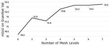
Figure 12: Ablation study: Multi-level feature refinement.

Mesh Simplification. In Section 3.6, we discuss two mesh simplification methods Vertex Clustering (VC) and Quadric Error Metrics (QEM) for multi-level feature learning. We apply the VC method on the first two mesh levels to remove high-frequency signals in noisy areas, and then apply the QEM method on the remaining mesh levels for its better topology-preserving property. To justify our choice, we train three models with the same network definition but performing on different mesh hierarchies, and compare their performances in Table VI (Right). “VC+QEM” refers to the mesh hierarchy simplified by the combination of the VC and QEM methods as described in Section 4.2. For “VC only”, at each mesh level $\mathcal{M}^{l}$, we set the cubical cell lengths of the VC method to the same size as the lengths of voxels in the corresponding voxel level $\mathcal{S}^{l}$. For “QEM only”, at each mesh level $\mathcal{M}^{l}$, the QEM method simplifies the mesh until the vertex number is reduced to 30% of its preceding mesh level $\mathcal{M}^{l-1}$. As shown in Table VI (Right), we witness a significant performance gap of 1.0% between the results of “VC+QEM” and “VC only”. We assume that the more faithful geodesic information provided by meshes simplified through the QEM method leads to the performance gain. We also notice that the performance of “QEM only” is slightly lower than the one of “VC+QEM”. It may be caused by the resulting high-frequency noises of directly applying the QEM method on the original meshes.

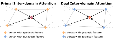
Figure 13: Illustration of primal and dual inter-domain attention. (Left) The primal inter-domain attention generates query vectors from the Euclidean features and aggregates the neighboring geodesic features. (Right) The dual inter-domain attention generates query vectors from the geodesic features and aggregates the neighboring Euclidean features.

Multi-level Feature Aggregation and Fusion. To measure the effects of individual geodesic feature refinement levels, we successively add the aggregation and fusion modules to the overall architecture. Except for the baseline with no geodesic branch, we start with the outermost mesh levels $\mathcal{M}^{0}\&\mathcal{M}^{1}$ to retain one fusion module and two aggregation modules. Next, along with each added mesh level, one fusion module and one aggregation module are added. The results are presented in Fig. 12. We witness that the first four levels bring the most performance gain, indicating the higher importance of finer-level meshes for geometric learning.

Design Choice of Inter-domain Attention. As described in Section 3.5, we proposed an inter-domain attentive module for adaptive feature fusion. The module takes both the Euclidean features and the geodesic features as input and utilizes the attention mechanism, in which the attention weights are conditioned on features from both the domains. To build such an inter-domain attentive module, there are two design choices.

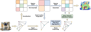
Figure 14: Network architecture Variant 1. Sharing the same encoder with VMNet, Variant 1 decodes the features in the Euclidean domain. For simplicity, only two levels of network are shown.

As shown in Fig. 13, we denote the one used in VMNet as the primal inter-domain attention and denote the other one as the dual inter-domain attention. We empirically find that the primal inter-domain attention yields better results than the dual one (73.3% vs 72.8% in mIoU on ScanNet Val). It may be caused by the different importance of the Euclidean features and the geodesic features in the task of indoor scene 3D semantic segmentation.

Design Choice of Network Architecture. As shown in Fig. 3, VMNet encodes contextual information in the Euclidean domain and then decodes the aggregated features in the geodesic domain. To justify our design choice, we construct two variants of VMNet.

Variant 1 (Fig. 14) shares the same encoder structure with VMNet. However, in the decoding part, instead of projecting the Euclidean features to the geodesic domain, Variant 1 projects the aggregated and fused geodesic features back to the Euclidean domain, and the per-voxel features on the last voxel level $S^{0}$ are used for semantic prediction. We compare the performances of Variant 1 and VMNet in Table VII. While having similar network complexity, Variant 1 performs significantly worse than our proposed VMNet. We speculate that the problem lies in the projection from vertices to voxels. To better preserve the geodesic information, we apply the QEM method to simplify the meshes resulting in non-uniform vertices. In the projection from vertices to voxels, multiple vertices thus correspond to a single voxel in areas with complex geometries and a voxel in areas with simple geometries may have no corresponding vertices at all. In contrast, projecting from uniform voxels to non-uniform vertices does not have this problem since all the vertices are covered and vertices sharing the same neighboring voxels have distinctive features through trilinear interpolation.

Variant 2 (Fig. 15) shares the same decoder structure with VMNet. In its encoding part, we incorporate both the voxel and mesh representations for contextual feature aggregation. As shown in Table VII, Variant 2 performs slightly better than our proposed VMNet (0.1% improvement in terms of mIoU) but brings considerable extra complexity. For a better complexity-performance trade-off, we prefer the proposed design choice of VMNet.

TABLE VII: Ablation study: Variants of network architecture.

Method	Params (M)	Latency (ms)	mIoU(%)
Variant 1	17.6	113	72.4
Variant 2	18.3	155	73.4
VMNet	17.5	107	73.3

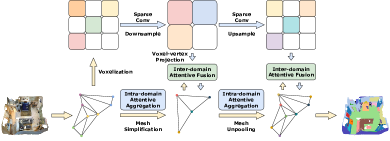
Figure 15: Network architecture Variant 2. Sharing the same decoder with VMNet, Variant 2 incorporates both the voxel and mesh representations for contextual feature encoding. For simplicity, only two levels of network are shown.

5 Conclusion

In this paper, we have presented a novel 3D deep architecture for semantic segmentation of indoor scenes, named Voxel-Mesh Network (VMNet). Aiming at addressing the problem of lacking consideration for the geodesic information in voxel-based methods, VMNet takes advantages of both the semantic contextual information available in voxels and the geometric surface information available in meshes to perform geodesic-aware 3D semantic segmentation. Extensive experiments show that VMNet achieves state-of-the-art results on the challenging ScanNet and Matterport3D datasets, significantly improving over strong baselines. We hope that our work will inspire further investigation of the idea of combining Euclidean and geodesic information, the development of new intra-domain and inter-domain modules, and the application of geodesic-aware networks to other tasks, such as 3D instance segmentation.

Zeyu Hu is a Ph.D. candidate in the Department of Computer Science and Engineering at the Hong Kong University of Science and Technology. Before joining HKUST, he received a Bachelor degree in Automation from University of Science and Technology of China in 2018. His primary research topic is about scene understanding.

Xuyang Bai is a Ph.D. candidate in the Department of Computer Science and Engineering at the Hong Kong University of Science and Technology. Before joining HKUST, he received a Bachelor degree in Electronic Information Science and Technology from Beijing Normal University in 2018. His primary research topic is about point cloud registration and LiDAR perception.

Jiaxiang Shang is a Ph.D. candidate in the Department of Computer Science and Engineering at the Hong Kong University of Science and Technology. Before joining HKUST, he had his Bachelor degree in the Department of Computer Science and Engineering at Sun Yat-sen University. His primary research topic is about face reconstruction.

Runze Zhang is currently a senior researcher of Tencent, Shenzhen, China. He received the Ph.D. degree from Hong Kong University of Science and Technology, in 2018. He received a Bachelor degree in Intelligence Science and Technology from the Peking University of China in 2013. His research interest is large-scale 3D reconstruction, including Structure-from-Motion, Multi-view Stereo, and other related topics.

Jiayu Dong received the B.S. degree in electronic information science and technology and the M.E. degree in computer science and technology from Sun Yatsen University, Guangzhou, China, in 2017 and 2020, respectively. His current research interests include face recognition and expression recognition.

Xin Wang is currently a senior researcher of Tencent, Shenzhen, China. He received the Ph.D. degree from the Sorbonne University, in 2017. His research interests include computer vision, computer graphics and their cross field.

Guangyuan Sun received the B.S. degree from Nanjing University, Nanjing, China, in 2004. He is currently a Senior Software Engineer with Tencent Lightspeed & Quantum Studios, Shenzhen, China. He has been dedicated to various applications of machine learning in game development for many years. His research interests include large-scale learning systems, reinforcement learning, and game theory.

Hongbo Fu is a Professor in the School of Creative Media, City University of Hong Kong. Before joining CityU, he had postdoctoral research training at the Imager Lab, University of British Columbia, Canada, and the Department of Computer Graphics, Max-Planck-Institut Informatik, Germany. He received a PhD degree in computer science from the Hong Kong University of Science and Technology in 2007 and a BS degree in information sciences from Peking University, China, in 2002. His primary research interests fall in the fields of computer graphics and human-computer interaction. He has served as an associate editor of The Visual Computer, Computers&Graphics, and Computer Graphics Forum.

Chiew-Lan Tai received the BSc degree in mathematics from the University of Malaya, the MSc degree in computer and information sciences from the National University of Singapore, and the DSc degree in information science from the University of Tokyo. She is currently a professor in the Department of Computer Science and Engineering at the Hong Kong University of Science and Technology. Her research interests include digital geometry processing, computer graphics, and computer vision.

TABLE VIII: Mean intersection over union scores on ScanNet Test [8]. This is a detailed version of Table 1 in the main paper.

Method	mIoU(%)	Conv Category	bathtub	bed	bookshelf	cabinet	chair	counter	curtain	desk	door	floor	otherfurniture	picture	refrigerator	shower curtain	sink	sofa	table	toilet	wall	window
TangentConv [58]	43.8	2D-3D	0.437	0.646	0.474	0.369	0.645	0.353	0.258	0.282	0.279	0.918	0.298	0.147	0.283	0.294	0.487	0.562	0.427	0.619	0.633	0.352
SurfaceConvPF [70]	44.2		0.505	0.622	0.380	0.342	0.654	0.227	0.397	0.367	0.276	0.924	0.240	0.198	0.359	0.262	0.366	0.581	0.435	0.640	0.668	0.398
3DMV [9]	48.3		0.484	0.538	0.643	0.424	0.606	0.310	0.574	0.433	0.378	0.796	0.301	0.214	0.537	0.208	0.472	0.507	0.413	0.693	0.602	0.539
TextureNet [23]	56.6		0.672	0.664	0.671	0.494	0.719	0.445	0.678	0.411	0.396	0.935	0.356	0.225	0.412	0.535	0.565	0.636	0.464	0.794	0.680	0.568
JPBNet [6]	63.4		0.614	0.778	0.667	0.633	0.825	0.420	0.804	0.467	0.561	0.951	0.494	0.291	0.566	0.458	0.579	0.764	0.559	0.838	0.814	0.598
MVPNet [25]	64.1		0.831	0.715	0.671	0.590	0.781	0.394	0.679	0.642	0.553	0.937	0.462	0.256	0.649	0.406	0.626	0.691	0.666	0.877	0.792	0.608
V-MVFusion [29]	74.6		0.771	0.819	0.848	0.702	0.865	0.397	0.899	0.699	0.664	0.948	0.588	0.330	0.746	0.851	0.764	0.796	0.704	0.935	0.866	0.728
BPNet [20]	74.9		0.909	0.818	0.811	0.752	0.839	0.485	0.842	0.673	0.644	0.957	0.528	0.305	0.773	0.859	0.788	0.818	0.693	0.916	0.856	0.723
PointNet++ [46]	33.9	PointConv	0.584	0.478	0.458	0.256	0.360	0.250	0.247	0.278	0.261	0.677	0.183	0.117	0.212	0.145	0.364	0.346	0.232	0.548	0.523	0.252
FCPN [47]	44.7		0.679	0.604	0.578	0.380	0.682	0.291	0.106	0.483	0.258	0.920	0.258	0.025	0.231	0.325	0.480	0.560	0.463	0.725	0.666	0.231
PointCNN [33]	45.8		0.577	0.611	0.356	0.321	0.715	0.299	0.376	0.328	0.319	0.944	0.285	0.164	0.216	0.229	0.484	0.545	0.456	0.755	0.709	0.475
DPC [13]	59.2		0.720	0.700	0.602	0.480	0.762	0.380	0.713	0.585	0.437	0.940	0.369	0.288	0.434	0.509	0.590	0.639	0.567	0.772	0.755	0.592
MCCN [19]	63.3		0.866	0.731	0.771	0.576	0.809	0.410	0.684	0.497	0.491	0.949	0.466	0.105	0.581	0.646	0.620	0.680	0.542	0.817	0.795	0.618
PointConv [67]	66.6		0.781	0.759	0.699	0.644	0.822	0.475	0.779	0.564	0.504	0.953	0.428	0.203	0.586	0.754	0.661	0.753	0.588	0.902	0.813	0.642
KPConv [59]	68.4		0.847	0.758	0.784	0.647	0.814	0.473	0.772	0.605	0.594	0.935	0.450	0.181	0.587	0.805	0.690	0.785	0.614	0.882	0.819	0.632
JSENet [21]	69.9		0.881	0.762	0.821	0.667	0.800	0.522	0.792	0.613	0.607	0.935	0.492	0.205	0.576	0.853	0.691	0.758	0.652	0.872	0.828	0.649
SparseConvNet [17]	72.5	SparseConv	0.647	0.821	0.846	0.721	0.869	0.533	0.754	0.603	0.614	0.955	0.572	0.325	0.710	0.870	0.724	0.823	0.628	0.934	0.865	0.683
MinkowskiNet [7]	73.6		0.859	0.818	0.832	0.709	0.840	0.521	0.853	0.660	0.643	0.951	0.544	0.286	0.731	0.893	0.675	0.772	0.683	0.874	0.852	0.727
SPH3D-GCN [32]	61.0	GraphConv	0.858	0.772	0.489	0.532	0.792	0.404	0.643	0.570	0.507	0.935	0.414	0.046	0.510	0.702	0.602	0.705	0.549	0.859	0.773	0.534
HPEIN [26]	61.8		0.729	0.668	0.647	0.597	0.766	0.414	0.680	0.520	0.525	0.946	0.432	0.215	0.493	0.599	0.638	0.617	0.570	0.897	0.806	0.605
DCM-Net [52]	65.8		0.778	0.702	0.806	0.619	0.813	0.468	0.693	0.494	0.524	0.941	0.449	0.298	0.510	0.821	0.675	0.727	0.568	0.826	0.803	0.637
VMNet (Ours)	74.6	Sparse+Graph Conv	0.870	0.838	0.858	0.729	0.850	0.501	0.874	0.587	0.658	0.956	0.564	0.299	0.765	0.900	0.716	0.812	0.631	0.939	0.858	0.709

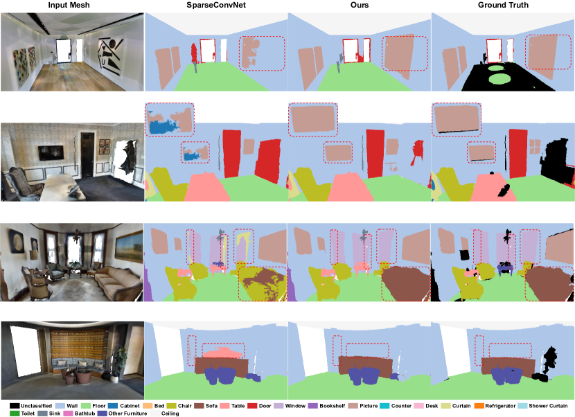
Figure 16: More qualitative results on Matterport3D Test [4]. The key parts for comparison are highlighted by dotted red boxes.

Figure 17: More qualitative results on ScanNet Val [8]. The key parts for comparison are highlighted by dotted red boxes.

References

- [1] Y. Ben-Shabat, M. Lindenbaum, and A. Fischer. 3dmfv: Three-dimensional point cloud classification in real-time using convolutional neural networks. IEEE RA-L, 3(4):3145–3152, 2018.
- [2] D. Boscaini, J. Masci, E. Rodolà, and M. Bronstein. Learning shape correspondence with anisotropic convolutional neural networks. In NeurIPS, pages 3189–3197, 2016.
- [3] A. Boulch, B. Le Saux, and N. Audebert. Unstructured point cloud semantic labeling using deep segmentation networks. 3DOR, 2:7, 2017.
- [4] A. Chang, A. Dai, T. Funkhouser, M. Halber, M. Niessner, M. Savva, S. Song, A. Zeng, and Y. Zhang. Matterport3d: Learning from rgb-d data in indoor environments. 3DV, 2017.
- [5] L. Chen, G. Papandreou, I. Kokkinos, K. Murphy, and A. L. Yuille. Deeplab: Semantic image segmentation with deep convolutional nets, atrous convolution, and fully connected crfs. IEEE TPAMI, 40(4):834–848, 2017.
- [6] H. Chiang, Y. Lin, Y. Liu, and W. H. Hsu. A unified point-based framework for 3d segmentation. In 3DV, pages 155–163, 2019.
- [7] C. Choy, J. Gwak, and S. Savarese. 4d spatio-temporal convnets: Minkowski convolutional neural networks. In CVPR, pages 3075–3084, 2019.
- [8] A. Dai, A. X. Chang, M. Savva, M. Halber, T. Funkhouser, and M. Nießner. Scannet: Richly-annotated 3d reconstructions of indoor scenes. In CVPR, 2017.
- [9] A. Dai and M. Nießner. 3dmv: Joint 3d-multi-view prediction for 3d semantic scene segmentation. In ECCV, pages 452–468, 2018.
- [10] A. Dai, M. Nießner, M. Zollhöfer, S. Izadi, and C. Theobalt. Bundlefusion: Real-time globally consistent 3d reconstruction using on-the-fly surface reintegration. ACM ToG, 36(4):1, 2017.
- [11] A. Dai, D. Ritchie, M. Bokeloh, S. Reed, J. Sturm, and M. Nießner. Scancomplete: Large-scale scene completion and semantic segmentation for 3d scans. In CVPR, pages 4578–4587, 2018.
- [12] M. Defferrard, X. Bresson, and P. Vandergheynst. Convolutional neural networks on graphs with fast localized spectral filtering. In NeurIPS, pages 3844–3852, 2016.
- [13] F. Engelmann, T. Kontogianni, and B. Leibe. Dilated point convolutions: On the receptive field size of point convolutions on 3d point clouds. In ICRA, pages 9463–9469, 2020.
- [14] M. Fey and J. E. Lenssen. Fast graph representation learning with PyTorch Geometric. In ICLR Workshop on Representation Learning on Graphs and Manifolds, 2019.
- [15] F. B. Fuchs, D. E. Worrall, V. Fischer, and M. Welling. Se(3)-transformers: 3d roto-translation equivariant attention networks. In NeurIPS, 2020.
- [16] M. Garland and P. S. Heckbert. Surface simplification using quadric error metrics. In SIGGRAPH, pages 209–216, 1997.
- [17] B. Graham, M. Engelcke, and L. van der Maaten. 3d semantic segmentation with submanifold sparse convolutional networks. In CVPR, pages 9224–9232, 2018.
- [18] L. Han, T. Zheng, L. Xu, and L. Fang. Occuseg: Occupancy-aware 3d instance segmentation. In CVPR, pages 2940–2949, 2020.
- [19] P. Hermosilla, T. Ritschel, P. Vázquez, À. Vinacua, and T. Ropinski. Monte carlo convolution for learning on non-uniformly sampled point clouds. ACM TOG, 37(6):1–12, 2018.
- [20] W. Hu, H. Zhao, L. Jiang, J. Jia, and T. Wong. Bidirectional projection network for cross dimension scene understanding. In CVPR, 2021.
- [21] Z. Hu, M. Zhen, X. Bai, H. Fu, and C. Tai. Jsenet: Joint semantic segmentation and edge detection network for 3d point clouds. In ECCV, pages 222–239, 2020.
- [22] B. Hua, M. Tran, and S. Yeung. Pointwise convolutional neural networks. In CVPR, pages 984–993, 2018.
- [23] J. Huang, H. Zhang, L. Yi, T. Funkhouser, M. Nießner, and L. J. Guibas. Texturenet: Consistent local parametrizations for learning from high-resolution signals on meshes. In CVPR, pages 4440–4449, 2019.
- [24] S. Huang, Z. Ma, T. Mu, H. Fu, and S. Hu. Supervoxel convolution for online 3d semantic segmentation. ACM TOG, 2021.
- [25] M. Jaritz, J. Gu, and H. Su. Multi-view pointnet for 3d scene understanding. In ICCVW, pages 0–0, 2019.
- [26] L. Jiang, H. Zhao, S. Liu, X. Shen, C. Fu, and J. Jia. Hierarchical point-edge interaction network for point cloud semantic segmentation. In ICCV, pages 10433–10441, 2019.
- [27] O. Kähler, V. A. Prisacariu, C. Y. Ren, X. Sun, P. Torr, and D. Murray. Very high frame rate volumetric integration of depth images on mobile devices. IEEE TVCG, 21(11):1241–1250, 2015.
- [28] A. Komarichev, Z. Zhong, and J. Hua. A-cnn: Annularly convolutional neural networks on point clouds. In CVPR, pages 7421–7430, 2019.
- [29] A. Kundu, X. Yin, A. Fathi, D. Ross, B. Brewington, T. Funkhouser, and C. Pantofaru. Virtual multi-view fusion for 3d semantic segmentation. In ECCV, pages 518–535, 2020.
- [30] F. J. Lawin, M. Danelljan, P. Tosteberg, G. Bhat, F. S. Khan, and M. Felsberg. Deep projective 3d semantic segmentation. In CAIP, pages 95–107, 2017.
- [31] H. Lei, N. Akhtar, and A. Mian. Octree guided cnn with spherical kernels for 3d point clouds. In CVPR, pages 9631–9640, 2019.
- [32] H. Lei, N. Akhtar, and A. Mian. Spherical kernel for efficient graph convolution on 3d point clouds. IEEE TPAMI, 2020.
- [33] Y. Li, R. Bu, M. Sun, W. Wu, X. Di, and B. Chen. Pointcnn: Convolution on x-transformed points. In NeurIPS, volume 31. Curran Associates, Inc., 2018.
- [34] Y. Li, X. Jin, J. Mei, X. Lian, L. Yang, C. Xie, Q. Yu, Y. Zhou, S. Bai, and A. L. Yuille. Neural architecture search for lightweight non-local networks. In CVPR, pages 10297–10306, 2020.
- [35] Z. Liu, H. Tang, Y. Lin, and S. Han. Point-voxel cnn for efficient 3d deep learning. In NeurIPS, pages 965–975, 2019.
- [36] J. Long, E. Shelhamer, and T. Darrell. Fully convolutional networks for semantic segmentation. In CVPR, pages 3431–3440, 2015.
- [37] J. Mao, X. Wang, and H. Li. Interpolated convolutional networks for 3d point cloud understanding. In ICCV, pages 1578–1587, 2019.
- [38] J. Masci, D. Boscaini, M. Bronstein, and P. Vandergheynst. Geodesic convolutional neural networks on riemannian manifolds. In ICCVW, pages 37–45, 2015.
- [39] D. Maturana and S. Scherer. Voxnet: A 3d convolutional neural network for real-time object recognition. In IEEE/RSJ IROS, pages 922–928, 2015.
- [40] F. Monti, D. Boscaini, J. Masci, E. Rodola, J. Svoboda, and M. M. Bronstein. Geometric deep learning on graphs and manifolds using mixture model cnns. In CVPR, pages 5115–5124, 2017.
- [41] A. Nekrasov, J. Schult, O. Litany, B. Leibe, and F. Engelmann. Mix3d: Out-of-context data augmentation for 3d scenes. In 3DV, 2021.
- [42] N. Parmar, A. Vaswani, J. Uszkoreit, L. Kaiser, N. Shazeer, A. Ku, and D. Tran. Image transformer. In ICML, pages 4055–4064, 2018.
- [43] A. Paszke, S. Gross, S. Chintala, G. Chanan, E. Yang, Z. DeVito, Z. Lin, A. Desmaison, L. Antiga, and A. Lerer. Automatic differentiation in pytorch. 2017.
- [44] C. R. Qi, H. Su, K. Mo, and L. J. Guibas. Pointnet: Deep learning on point sets for 3d classification and segmentation. In CVPR, pages 652–660, 2017.
- [45] C. R. Qi, H. Su, M. Nießner, A. Dai, M. Yan, and L. J. Guibas. Volumetric and multi-view cnns for object classification on 3d data. In CVPR, pages 5648–5656, 2016.
- [46] C. R. Qi, L. Yi, H. Su, and L. J. Guibas. Pointnet++: Deep hierarchical feature learning on point sets in a metric space. In NeurIPS, pages 5099–5108, 2017.
- [47] D. Rethage, J. Wald, J. Sturm, N. Navab, and F. Tombari. Fully-convolutional point networks for large-scale point clouds. In ECCV, pages 596–611, 2018.
- [48] G. Riegler, A. Osman Ulusoy, and A. Geiger. Octnet: Learning deep 3d representations at high resolutions. In CVPR, pages 3577–3586, 2017.
- [49] O. Ronneberger, P. Fischer, and T. Brox. U-net: Convolutional networks for biomedical image segmentation. In MICCAI, pages 234–241, 2015.
- [50] J. Rossignac and P. Borrel. Multi-resolution 3d approximations for rendering complex scenes. In Modeling in computer graphics, pages 455–465. Springer, 1993.
- [51] X. Roynard, J. Deschaud, and F. Goulette. Classification of point cloud scenes with multiscale voxel deep network. arXiv preprint arXiv:1804.03583, 2018.
- [52] J. Schult, F. Engelmann, T. Kontogianni, and B. Leibe. Dualconvmesh-net: Joint geodesic and euclidean convolutions on 3d meshes. In CVPR, pages 8612–8622, 2020.
- [53] Y. Shi, Z. Huang, S. Feng, and Y. Sun. Masked label prediction: Unified massage passing model for semi-supervised classification. arXiv preprint arXiv:2009.03509, 2020.
- [54] M. Simonovsky and N. Komodakis. Dynamic edge-conditioned filters in convolutional neural networks on graphs. In CVPR, pages 3693–3702, 2017.
- [55] S. Song, F. Yu, A. Zeng, A. X. Chang, M. Savva, and T. Funkhouser. Semantic scene completion from a single depth image. In CVPR, pages 1746–1754, 2017.
- [56] H. Su, V. Jampani, D. Sun, S. Maji, E. Kalogerakis, M. Yang, and J. Kautz. Splatnet: Sparse lattice networks for point cloud processing. In CVPR, pages 2530–2539, 2018.
- [57] H. Tang, Z. Liu, S. Zhao, Y. Lin, J. Lin, H. Wang, and S. Han. Searching efficient 3d architectures with sparse point-voxel convolution. In ECCV, pages 685–702, 2020.
- [58] M. Tatarchenko, J. Park, V. Koltun, and Q. Zhou. Tangent convolutions for dense prediction in 3d. In CVPR, pages 3887–3896, 2018.
- [59] H. Thomas, C. R. Qi, J. Deschaud, B. Marcotegui, F. Goulette, and L. J. Guibas. Kpconv: Flexible and deformable convolution for point clouds. In ICCV, pages 6411–6420, 2019.
- [60] A. Vaswani, N. Shazeer, N. Parmar, J. Uszkoreit, L. Jones, A. N. Gomez, L. Kaiser, and I. Polosukhin. Attention is all you need. In NeurIPS, volume 30, 2017.
- [61] L. Wang, Y. Huang, Y. Hou, S. Zhang, and J. Shan. Graph attention convolution for point cloud semantic segmentation. In CVPR, pages 10296–10305, 2019.
- [62] P. Wang, Y. Liu, Y. Guo, C. Sun, and X. Tong. O-cnn: Octree-based convolutional neural networks for 3d shape analysis. ACM TOG, 2017.
- [63] Y. Wang, Y. Sun, Z. Liu, S. E. Sarma, M. M. Bronstein, and J. M. Solomon. Dynamic graph cnn for learning on point clouds. ACM TOG, 38(5):1–12, 2019.
- [64] Z. Wang and F. Lu. Voxsegnet: Volumetric cnns for semantic part segmentation of 3d shapes. IEEE TVCG, 2019.
- [65] T. Whelan, R. F. Salas-Moreno, B. Glocker, A. J. Davison, and S. Leutenegger. Elasticfusion: Real-time dense slam and light source estimation. The International Journal of Robotics Research, 35(14):1697–1716, 2016.
- [66] C. Wong and C. Vong. Efficient outdoor 3d point cloud semantic segmentation for critical road objects and distributed contexts. In ECCV, pages 499–514. 2020.
- [67] W. Wu, Z. Qi, and F. Li. Pointconv: Deep convolutional networks on 3d point clouds. In CVPR, pages 9621–9630, 2019.
- [68] Z. Wu, S. Song, A. Khosla, F. Yu, L. Zhang, X. Tang, and J. Xiao. 3d shapenets: A deep representation for volumetric shapes. In CVPR, pages 1912–1920, 2015.
- [69] X. Yan, C. Zheng, Z. Li, S. Wang, and S. Cui. Pointasnl: Robust point clouds processing using nonlocal neural networks with adaptive sampling. In CVPR, pages 5589–5598, 2020.
- [70] Y. Yang, S. Liu, H. Pan, Y. Liu, and X. Tong. Pfcnn: convolutional neural networks on 3d surfaces using parallel frames. In CVPR, pages 13578–13587, 2020.
- [71] C. Zhang, W. Luo, and R. Urtasun. Efficient convolutions for real-time semantic segmentation of 3d point clouds. In IEEE 3DV, pages 399–408, 2018.
- [72] H. Zhao, L. Jiang, C. Fu, and J. Jia. Pointweb: Enhancing local neighborhood features for point cloud processing. In CVPR, pages 5565–5573, 2019.
- [73] H. Zhao, L. Jiang, J. Jia, P. Torr, and V. Koltun. Point transformer. arXiv preprint arXiv:2012.09164, 2020.
- [74] Y. Zhou and O. Tuzel. Voxelnet: End-to-end learning for point cloud based 3d object detection. In CVPR, pages 4490–4499, 2018.