DCG: Distributed Conjugate Gradient for Efficient Linear Equations Solving

Abstract

Distributed algorithms to solve linear equations in multi-agent networks have attracted great research attention and many iteration-based distributed algorithms have been developed. The convergence speed is a key factor to be considered for distributed algorithms, and it is shown dependent on the spectral radius of the iteration matrix. However, the iteration matrix is determined by the network structure and is hardly pre-tuned, making the iterative-based distributed algorithms may converge very slowly when the spectral radius is close to 1. In contrast, in centralized optimization, the Conjugate Gradient (CG) is a widely adopted idea to speed up the convergence of the centralized solvers, which can guarantee convergence in fixed steps. In this paper, we propose a general distributed implementation of CG, called DCG. DCG only needs local communication and local computation, while inheriting the characteristic of fast convergence. DCG guarantees to converge in $4Hn$ rounds, where $H$ is the maximum hop number of the network and $n$ is the number of nodes. We present the applications of DCG in solving the least square problem and network localization problem. The results show the convergence speed of DCG is three orders of magnitude faster than the widely used Richardson iteration method.

I Introduction

In many multi-agent applications, the underlying problem can be reduced to solving a system of linear equations[1]. Because the autonomous networked agents are usually discretely deployed, each agent only has the access to communicate with direct neighbors. Moreover, in certain scenarios, each agent only desires its own state. Such characteristics consequently give rise to distributed solvers for linear systems. Different from the centralized solvers, distributed solvers usually adopt iterative manners. The key feature of iterative approaches is linear iterations, where each agent receives states of direct neighbors; updates and sends its own state. The barycentric linear localization algorithm[2], is a typical iteration-based method.

The convergence speed is a crucial factor of the iteration-based distributed algorithms, which determines whether the distributed algorithm can be used when the application requires a fast response. However, the convergence rate of many iterative methods, e.g., Jacobi iteration, Gauss-Seidel iteration, and Richardson iteration[3], are characterized by the spectral radius of the iteration matrix. However, the spectral radius is determined by the network topology and is difficult to be pre-tuned. Thus the convergence speed is highly uncertain and may be very slow in some network states.

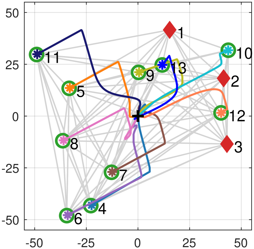
(a) The Richardson Iteration

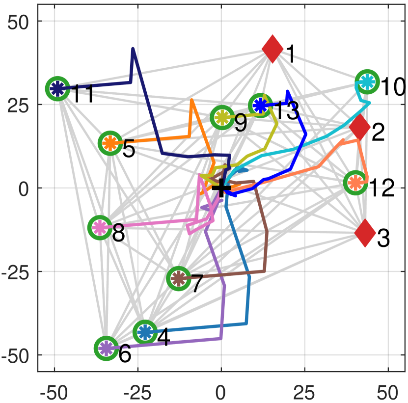
(b) DCG

Figure 1: The convergence trails in $\mathbb{R}^{2}$. The marker ‘+’ represents the start a trail. The marker ‘$*$’ and ‘$\circ$’ represent the converged estimation $\mathbf{\hat{x}}_{i}$ and the ground truth $\mathbf{x}_{i}$, respectively.

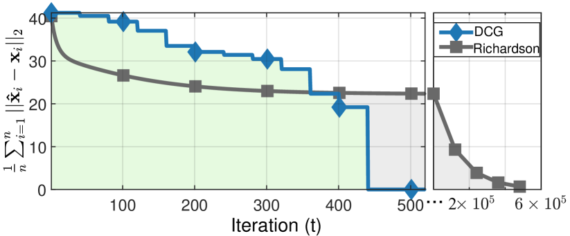
Figure 2: The mean square error w.r.t. iteration rounds.

To guarantee fast convergence of distributed algorithms in solving linear equations, this study explores the idea of Conjugate Gradient (CG)[4]. CG has two desired properties for solving the linear systems: 1) CG converges to the exact solution after a finite number of iterations, which is not larger than the size of the system matrix; 2) CG is suited for solving linear systems with large and sparse system matrices. But CG is essentially a centralized solver. In pursuit of distributed implementation, we design an efficient protocol to synchronize the necessary vectors to update the residual. Our distributed CG, i.e., DCG remarkably speeds up convergence by paying limited neighborhood communication costs.

The rest of the paper is organized as follows. We formulate the problem and present related algorithms in Section II. DCG is proposed in Section III. Applications of DCG are discussed in Section IV. DCG is evaluated in Section V. The paper is concluded with further discussions in Section VI.

Notations: Throughout the paper, let $\mathbf{AX=b}$ denote a system of linear equations, where $\mathbf{A}\in\mathbb{R}^{n\times n}$ is the coefficient matrix, $\mathbf{b}\in\mathbb{R}^{n\times d}$ is the right-hand side vector, and $\mathbf{X}\in\mathbb{R}^{n\times d}$ is the vector of unknowns. $n$ is the number of variables and $d$ is the spatial dimension of a vector, $d\in\{2,3\}$. The vector $\mathbf{A}_{i,:}=[A_{i1}\cdots A_{in}]$ denotes the $i$th row of $\mathbf{A}$, $i\in\{1\cdots n\}$.

II Preliminaries

II-A Problem Formulation

Consider a network of $n$ agents $\mathcal{V}=\{v_{1},\cdots,v_{n}\}$, each agent $v_{i}$ is capable of communicating with the agents within its reception range $R$. Let $\mathcal{E}$ be the set of edges and $(i,j)\in\mathcal{E}$ if the distance between $v_{i}$ and $v_{j}$ is not larger than $R$. Then the multi-agent network can be represented as a graph $\mathcal{G=(V,E)}$. The neighbors of $v_{i}$ is denoted by $\mathcal{N}_{i}$, $j\in\mathcal{N}_{i}$ if $(i,j)\in\mathcal{E}$.

Problem: Assume that $\mathbf{A}$ is non-singular. Let $\mathbf{X}^{*}$ denote the unique solution satisfying $\mathbf{AX=b}$. Suppose each agent $v_{i}$ holds a state vector $\mathbf{\hat{x}}_{i}\in\mathbb{R}^{d}$. Initially, $v_{i}$ knows $\mathbf{\mathbf{A}}_{i,:}$ and $\mathbf{\mathbf{b}}_{i,:}$. The problem is to devise a local rule for each agent to update its state $\mathbf{\hat{x}}_{i}$ leveraging the local communication with agents in $\mathcal{N}_{i}$ so that $\mathbf{\hat{x}}_{i}(t)$ converges to $\mathbf{x}^{*}_{i}$ within finite $t$.

II-B Related Work

The basic idea of the iterative methods is as follows. Given an initialization $\mathbf{\hat{x}}(0)$, generate an iteration sequence $\{\mathbf{\hat{x}}(t)\}_{t=0}^{\infty}$ in a certain manner, so that:

$$\lim\limits_{t\to\infty}\mathbf{\hat{x}}(t)=\mathbf{x}^{*}\triangleq\mathbf{A}^{-1}\mathbf{b}.$$ (1)

Generally, the state update of an iterative method can be represented as:

$$\mathbf{\hat{x}}(t+1)=\phi_{k}(\mathbf{\hat{x}}(t),\mathbf{\hat{x}}(t-1)\cdots,\mathbf{\hat{x}}(0),\mathbf{A},\mathbf{b}),$$ (2)

where $\mathbf{\hat{x}}(0)=\phi_{0}(\mathbf{A},\mathbf{b)}$ or $\mathbf{\hat{x}}(0)$ is selected manually. $\phi_{k}$ is called the iteration function. The specific design of iterative functions are based on the matrix splitting.

Definition 1 (Matrix Splitting).

Suppose a non-singular matrix $\mathbf{A}\in\mathbb{R}^{n\times n}$, a split of matrix $\mathbf{A}$ is defined as $\mathbf{A}=\mathbf{M}-\mathbf{N}$, where $\mathbf{M}$ is also non-singular.

Consider a general linear system:

$$\mathbf{AX=b},$$ (3)

where $\mathbf{A}$ is non-singular. (3) can be transformed as follows through matrix splitting $\mathbf{A}=\mathbf{M}-\mathbf{N}$.

$$\mathbf{M{X}=N{X}+b}.$$ (4)

Then, we can construct an iteration function as:

$$\mathbf{M\hat{X}}(t+1)=\mathbf{N\hat{X}}(t)+\mathbf{b},$$ (5)

which is equivalent to:

$$\mathbf{\hat{X}}(t+1)=\mathbf{M}^{-1}\mathbf{N\hat{X}}(t)+\mathbf{M}^{-1}\mathbf{b}\triangleq\mathbf{G\hat{X}}(t)+\mathbf{g}.$$ (6)

$\mathbf{G}=\mathbf{M}^{-1}\mathbf{b}$ is called the iteration matrix. It is straightforward that different iterative methods can be constructed by varying $\mathbf{M}$.

In Jacobi iteration, $\mathbf{A}$ is splitted as:

$$\mathbf{A=D-L-U}.$$ (7)

$\mathbf{D}$ is the diagonal component of $\mathbf{A}$. $-\mathbf{L}$ and $-\mathbf{U}$ are the upper triangle component and the lower triangle component of $\mathbf{A}$, respectively. Then, the Jacobi iteration is specified as:

$$\mathbf{\hat{X}}(t+1)=\mathbf{D}^{-1}(\mathbf{L}+\mathbf{U})\mathbf{\hat{X}}(t)+\mathbf{D}^{-1}\mathbf{b}.$$ (8)

From the local behavior of an individual agent $v_{i}$, the state update is:

$$\mathbf{\hat{x}}_{i}(t+1)=\frac{1}{A_{ii}}\left(\mathbf{b}_{i}-\sum\limits_{j=1,j\neq i}^{n}A_{ij}\mathbf{\hat{x}}_{j}(t)\right)$$ (9)

In Gauss-Seidel iteration, the iteration function is designed as:

$$\mathbf{\hat{X}}(t+1)=(\mathbf{D-L})^{-1}\mathbf{U}\mathbf{\hat{X}}(t)+(\mathbf{D-L})^{-1}\mathbf{b}.$$ (10)

The local update of agent $v_{i}$’s state is:

$$\mathbf{\hat{x}}_{i}(t+1)=\frac{1}{A_{ii}}\left(\mathbf{b}_{i}-\sum\limits_{j=1}^{i-1}A_{ij}\mathbf{\hat{x}}_{j}(t+1)-\sum\limits_{j=i+1}^{n}A_{ij}\mathbf{\hat{x}}_{j}(t)\right)$$ (11)

Another brief iteration method is the Richardson iteration when $\mathbf{A}$ is symmetric positive definite. The iteration function is:

$$\mathbf{\hat{X}}(t+1)=\mathbf{\hat{X}}(t)+\omega(\mathbf{b}-\mathbf{A}\mathbf{\hat{X}}(t)).$$ (12)

The state of agent $v_{i}$ is updated as:

$$\mathbf{\hat{x}}_{i}(t+1)=\mathbf{\hat{x}}_{i}(t)+\omega\left(\mathbf{b}_{i}-\sum\limits_{j=1}^{n}\mathbf{A}_{ij}\mathbf{\hat{x}}_{j}(t)\right),$$ (13)

where $\omega$ is a non-negative scalar and is suggested to be $\frac{2}{\lambda_{max}+\lambda_{min}}$. Similar methods include the Successive Over-Relaxation (SOR) iteration, the Symmetric SOR (SSOR) iteration, the Accelerated OR (AOR) iteration, the Symmetric AOR (SAOR) etc [5].

II-C Convergence and Convergence Rate

Since the aforementioned methods are iterative, a crucial issue is to guarantee iteration convergence. For a general iteration function as in (6), its convergence is guaranteed by the following theorem.

Theorem 1.

The iterates formulated by $\mathbf{\hat{X}}(t+1)=\mathbf{G}\mathbf{\hat{X}}(t)+\mathbf{b}$ converges for any $\mathbf{\hat{X}}(0)$, if and only if $\rho(\mathbf{G})<1$[6].

$\rho(\mathbf{G})$ is the spectral radius of the iteration matrix $\mathbf{G}$. See Theorem 4.1 of [6] for the proof.

Apart from knowing when the iteration converges, it is also desirable to explore how fast it converges. Saad [6] presented that the convergence rate $\tau$ is the natural logarithm of the inverse of the spectral radius:

$$\tau=\ln\frac{1}{\rho(\mathbf{G})}=-\ln\rho(\mathbf{G}).$$ (14)

It can be seen that these iterative methods converge slowly when $\mathbf{G}$ has unstable eigenvalues.

III DCG: A General Distributed Conjugate Gradient Implementation

The most attractive feature of CG is that it converges within a fixed round of iterations. But CG is essentially a centralized gradient-based solver for linear equations. See Section 6 of [6] for the original CG algorithm. Although parallel or distributed CG algorithms have been reported for allocating computational loads in cloud computing[7] and estimating spectrum in sensor networks[8], the general distributed CG has not been well touched.

The key difficulty in implementing Distributed CG (DCG) is that the state $\widehat{X}_{i}$ is updated based on several vectors, however, $v_{i}$ only knows the $i$th element of these vectors. Specifically, $\widehat{X}_{i}(t)=\widehat{X}_{i}(t-1)+\alpha_{i}(t){d}_{i}(t)$. $\alpha_{i}(t)$ and $d_{i}(t)$ are calculated using the direction vector $\mathbf{d}(t)$ and the residual vector $\mathbf{r}(t)$. But $v_{i}$ only knows $d_{i}$ and $r_{i}$.

III-A Vector Synchronization

To supplement the necessary information, we design the Synchronize_Vector($z_{i}$) protocol, through which $v_{i}$ can gather any complete vector $\mathbf{z}$ by constantly exchanging respective elements with neighbors (Line 1-1 of Algorithm 1). $H$ is the largest number of hops throughout the network. So the synchronization can be finished in $H$ rounds. $H$ can be set to $n$ if it is not given at network deployment. The operation ‘merge’ (Line 1) means selecting all non-zero elements of the input vectors and stacking them as a new vector while maintaining their original indexes.

III-B Distributed Conjugate Gradient

DCG is detailed as Function DCG (Line 1-1 of Algorithm 1). At initialization (Line 1), the state $\widehat{X}_{i}(0)$ is set to 0. The direction vector component ${d}_{i}$ and the residual vector component ${r}_{i}$ are set to 0 and $-{b}_{i}$, respectively. At each iteration $t$, the local behavior of a node $v_{i}$ is as follows:

• Update Residual (Line 1). The residual ${r}_{i}$ is updated by ${r}_{i}(t)=(\mathbf{\mathbf{A}\widehat{X}})_{i}(t-1)-{b}_{i}$, which is realized by ${r}_{i}(t)=-b_{i}+\sum\nolimits_{j\in\mathcal{N}_{i}}\mathbf{A}_{ij}\widehat{X}_{j}(t-1)$. $\mathbf{\mathbf{A}}_{(i,:)}$ and $b_{i}$ are known to $v_{i}$ at the begining. $\widehat{X}_{j}(t-1)$ is the state of neighbor $v_{j}$ obtained by local communication.

• Check Residual (Line 1). CG theoretically completes after $n$ iterations [3]. However, due to the accumulated floating point rounding off errors, the residual and the direction gradually lose accuracy. Thus, DCG terminates by checking whether $\mathbf{r}(t)^{T}\mathbf{r}(t)<\varepsilon$. The threshold $\varepsilon$ is an empirical value based on accuracy requirement. $\mathbf{r}(t)$ is obtained by: $\mathbf{r}(t)=$ Synchronize_Vector($r_{i}(t)$). After knowing the synchronized $\mathbf{r}$, the squared residual is calculated as $\mathbf{r}(t)^{T}\mathbf{r}(t)=\sum_{i=1}^{n}r_{i}(t)^{2}$.

• Update Direction (Line 1). $d_{i}$ needs another vector $\mathbf{r}(t-1)$ to be updated. It is obtained by Synchronize_Vector($r_{i}(t-1)$). Then, $\mathbf{r}(t-1)^{T}\mathbf{r}(t-1)=\sum_{i=1}^{n}r_{i}(t-1)^{2}$ and $d_{i}$ can be calculated locally.

• Update Step Size (Line 1). Represent the numerator and denominator of $\alpha_{i}$ as $numer=\mathbf{d}(t)^{T}\mathbf{r}(t)$ and $denom=\mathbf{d}(t)^{T}\mathbf{\mathbf{A}}\mathbf{d}(t)$, respectively. The direction vector $\mathbf{d}(t)$ is obtained by Synchronize_Vector($d_{i}(t)$). So the numerator can be known as $numer=\sum_{i=1}^{n}d_{i}(t)r_{i}(t)$.

  An intermediate vector $\mathbf{T}(t)=[T_{1}(t)\cdots T_{n}(t)]^{T}$ is introduced to calculate $denom$. By communicating with neighbors, $v_{i}$ calculates ${T}_{i}(t)=\sum\nolimits_{j\in\mathcal{N}_{i}}\mathbf{A}_{ij}{d}_{j}(t)$. The complete $\mathbf{T}(t)$ is obtained by Synchronize_Vector($T_{i}(t)$). So $denom=\sum\nolimits_{i=1}^{n}d_{i}(t)T_{i}(t)$. Then $\alpha_{i}=-numer/denom$.

• Update State (Line 1). The state $\widehat{X}_{i}(t)$ updates a step $\alpha_{i}(t){d}_{i}(t)$ along its last state.

Overall, all of the above DCG procedures are completely distributed and implemented through neighborhood message passing.

Input: $\mathbf{\Omega}_{(i,:)}$; $b_{i}$;

Output: $\mathbf{\hat{x}}_{i}$;

1

2 $\widehat{X}_{i}(0)\leftarrow 0$; ${d}_{i}(0)\leftarrow 0$; ${r}_{i}(0)\leftarrow-b_{i}$ // Initialize

/* Update $\widehat{X}_{i}$ as in Section III-B */

43 for iterations $t\in\{1,\cdots,t_{max}\}$ do

      5 ${r}_{i}(t)=(\mathbf{\Omega\widehat{X}}(t-1))_{i}-{b}_{i}$; // residual

7      6 if $\mathbf{r}(t)^{T}\mathbf{r}(t)<\varepsilon$ then

            8 break // meets accuracy requirement

9            

11      10${d}_{i}(t)$=$-{r}_{i}(t)$+$\frac{\mathbf{r}(t)^{T}\mathbf{r}(t)}{\mathbf{r}(t-1)^{T}\mathbf{r}(t-1)}$${d}_{i}(t-1)$ $//$direction

      12 $\alpha_{i}(t)=-\frac{\mathbf{d}(t)^{T}\mathbf{r}(t)}{\mathbf{d}(t)^{T}\mathbf{\Omega}\mathbf{d}(t)}$; // step size

      13 $\widehat{X}_{i}(t)=\widehat{X}_{i}(t-1)+\alpha_{i}(t){d}_{i}(t)$; // state

14      

1615 return $\widehat{X}_{i}(t)$.

17 Function Synchronize$\_$Vector($z_{i}$)

1918 initialize $\mathbf{z}_{i}(0)$ $\leftarrow$ $[\boldsymbol{0}_{(i-1)\times 1}~{}z_{i}~{}\boldsymbol{0}_{(n-i)\times 1}]$;

2120 for iterations $k\in\{0,\cdots,H\}$ do

23      22 exchange $\mathbf{z}_{i}(k)$ with $\mathcal{N}_{i}$;

25      24 for each $v_{j}\in\mathcal{N}_{i}$ do

27            26 $\mathbf{z}_{i}(k+1)$ $\leftarrow$ merge($\mathbf{z}_{i}(k)$, $\mathbf{z}_{j}(k)$);

28            

29      

3130return $\mathbf{z}_{i}$.

Algorithm 1 Distributed Conjugate Gradient (DCG) of $v_{i}$

III-C Analysis of DCG

In each round, four vectors are obtained by synchronization, so it converges within $4Hn$ rounds when $\mathbf{A}$ is non-singular. In actual applications, there may exist measurement noise so that $\mathbf{A}$ and $\mathbf{b}$ are influenced and the constructed linear system may be unsolvable[9]. Let $\overline{\mathbf{A}}$ and $\overline{\mathbf{b}}$ denote the noisy matrices as:

$$\overline{\mathbf{A}}=\mathbf{A}+\Delta\mathbf{A},\overline{\mathbf{b}}=\mathbf{b}+\Delta\mathbf{b},$$ (15)

where $\Delta\mathbf{A}$ and $\Delta\mathbf{b}$ are error matrices implying the noise. If the noisy matrix $\overline{\mathbf{A}}$ is still non-singular, DCG still converges to the neighborhood of $\mathbf{X}^{*}$.

Lemma 1.

For a noisy linear system $\overline{\mathbf{A}}\mathbf{X}=\mathbf{b}$, DCG converges if the error matrix satisfies:

$$||\Delta\mathbf{A}||<\lambda_{min}(\mathbf{A}).$$ (16)

Proof.

From (15), we can obtain:

$$\overline{\mathbf{A}}=\mathbf{A}(I+\mathbf{A}^{-1}\Delta\mathbf{A}).$$ (17)

Since $||\mathbf{A}^{-1}\Delta\mathbf{A}||\leq||\mathbf{A}^{-1}||~{}||\Delta\mathbf{A}||=\frac{||\Delta\mathbf{A}||}{\lambda_{min}(\mathbf{A})}$, the matrix $\overline{\mathbf{A}}$ must be non-singular if (16) holds. Thus DCG can converge to the neighborhood of $\mathbf{X}^{*}$ shown as: $\mathbf{\overline{X}}^{*}=\overline{\mathbf{A}}^{-1}\overline{\mathbf{b}}$. ∎

IV Applications of DCG

In this section, we investigate applying DCG to two actual scenarios.

IV-A The Least Square Problem

Linear equations arising from the era of engineering are usually over-determined. A typical scenario is distributed parameter estimation, where the observation equations are as:

$$A_{i}x_{i}=b_{i}+\delta_{i},$$ (18)

where $x_{i}$ is the desired parameter to be calculated and $\delta_{i}$ is the component implying the measurement noise of $b_{i}$. Due to the measurement noise, such linear equations usually do not have a solution that exactly meets the constraints. This problem can be formulated as follows. Suppose there is no solution to the linear system $\mathbf{AX=b}$ and $\mathbf{AA}^{T}$ is non-singular. Each agent $v_{i}$ only knows the $i$th row of $\mathbf{A}$ and $\mathbf{b}$, which are denoted by $\mathbf{A}_{i,:}$ and $\mathbf{b}_{i,:}$, respectively. Design a distributed rule for each agent to update its state $\mathbf{x}_{i}$ so that $\mathbf{x}_{i}(t)$ converges to the unique solution of:

$$\mathbf{A}^{T}\mathbf{AX}=\mathbf{A}^{T}\mathbf{b}.$$ (19)

Let $\boldsymbol{\Omega}=\mathbf{A}^{T}\mathbf{A}$ and $\boldsymbol{\beta}=\mathbf{A}^{T}\mathbf{b}$. To solve the least square problem as in (19), each agent should be aware of the $i$th row of $\boldsymbol{\Omega}$ and $\boldsymbol{\beta}$ using $\mathbf{A}_{i,:}$ and $\mathbf{b}_{i,:}$.

Initially, $v_{i}$ maintains $\mathbf{A}_{i,:}$.Then, $v_{i}$ transmits ${A}_{i,j}$ to $\mathcal{N}_{i}$ and receives ${A}_{j,i}$ from $\mathcal{N}_{i}$, then it also knows the nonzero elements of the $i$th column $\mathbf{A}_{:,i}$, i.e., $\mathbf{A}^{T}_{i,:}$. Thus the nonzero elements of $\boldsymbol{\Omega}_{i,:}$ are calculated distributively as:

$${\Omega}_{ij}=\sum\nolimits_{k=1}^{n}{A}^{T}_{ik}A_{kj},\forall v_{j}\in\mathcal{N}_{i}.$$ (20)

Similarly, $\boldsymbol{\beta}_{i,:}$ can be calculated as:

$${\beta}_{ij}=\sum\nolimits_{k=1}^{n}{A}^{T}_{ik}b_{kj},j\in\{1,\cdots,d\}.$$ (21)

Finally, the problem can be solved as $\mathbf{x}_{i}=DCG(\boldsymbol{\Omega}_{i,:},\boldsymbol{\beta}_{i,:})$. Therefore $\mathbf{x}$ solves the least squares problem in (19).

IV-B The Network Localization Problem

The geographical locations of nodes are fundamental information for many multi-agent applications[10, 11, 12]. Network localization techniques are usually adopted for calculating node locations in infrastructure-less scenarios[13, 14], which are formulated as follows. For a network of $m+n$ agents in $\mathbb{R}^{d}$, let $\mathcal{V}=\mathcal{A}\cup\mathcal{F}$ denote the entire node set. Nodes in $\mathcal{A}=\{v_{1},\cdots,v_{m}\}$ are called anchor agents, whose locations $\mathbf{P}_{\mathcal{A}}=\{\mathbf{p}_{1},\cdots,\mathbf{p}_{m}\}$ are known. Nodes in $\mathcal{F}=\{v_{m+1},\cdots,v_{m+n}\}$ are called free agents, whose locations $\mathbf{P}_{\mathcal{F}}=\{\mathbf{p}_{m+1},\cdots,\mathbf{p}_{m+n}\}$ are unknown. Each agent $v_{i}$ can only sense the relative distance $d_{ij}$ between $v_{i}$ and any neighbor $v_{j}\in\mathcal{N}_{i}$. Each agent can exchange its estimated location $\hat{\mathbf{p}}_{i}$ and distance measurements with neighbors. The network localization problem is to design a distributed protocol for each agent to update its location $\hat{\mathbf{p}}_{i}$ so that it converges to $\mathbf{p}_{i}$.

To solve the network localization problem, we transform it to a linear system. First, each location $\mathbf{p}_{i}$ is represented as a linear combination of locations of neighbors:

$$\mathbf{p}_{i}=\sum_{v_{j}\in\mathcal{N}_{i}}a_{ij}\mathbf{p}_{j},$$ (22)

where $a_{ij}$ are called barycentric coordinates. The calculation of barycentric coordinates involve only local distance measurements and the specific process is introduced by Diao et al. [2] in $\mathbb{R}^{2}$ and by Han et al. [15] in $\mathbb{R}^{3}$. Then after calculating the barycentric coordinates for each node, the agent locations can form a linear system:

$$\left[{\begin{array}[]{*{20}{c}}{{{\mathbf{P}}_{\mathcal{A}}}}\\ {{{{\mathbf{P}}}_{\mathcal{F}}}}\end{array}}\right]=\left[{\begin{array}[]{*{20}{c}}{\mathbf{I}}&{\mathbf{0}}\\ {\mathbf{B}}&{\mathbf{C}}\end{array}}\right]\left[{\begin{array}[]{*{20}{c}}{{{\mathbf{P}}_{\mathcal{A}}}}\\ {{{{\mathbf{P}}}_{\mathcal{F}}}}\end{array}}\right].$$ (23)

$\mathbf{A}=\left[{\begin{array}[]{*{20}{c}}{\mathbf{I}}&{\mathbf{0}}\\ {\mathbf{B}}&{\mathbf{C}}\end{array}}\right]\in\mathbb{R}^{(m+n)\times(m+n)}$ is constructed with barycentric coordinates, i.e., the $i$th row of $\mathbf{A}$ is the barycentric coordinate of $v_{i}$ w.r.t. its neighbors $\mathcal{N}_{i}$. Then, the localization problem can be transformed into solving the following linear system:

$$(\mathbf{I}-\mathbf{C})\mathbf{P}_{\mathcal{F}}=\mathbf{B}\mathbf{P}_{\mathcal{A}}.$$ (24)

Writing $\mathbf{I}-\mathbf{C}$ as $\mathbf{M}$, (24) can be reformulated as:

$$\mathbf{M}\mathbf{P}_{\mathcal{F}}=\mathbf{B}\mathbf{P}_{\mathcal{A}}.$$ (25)

Considering that CG is used when the system matrix is positive definite [3]. Thus, we multiply $\mathbf{M}^{T}$ to both sides of (25):

$$\mathbf{M}^{T}\mathbf{M}\mathbf{P}_{\mathcal{F}}=\mathbf{M}^{T}\mathbf{B}\mathbf{P}_{\mathcal{A}}.$$ (26)

Then, $\mathbf{M}^{T}\mathbf{M}$ is positive definite. To apply DCG to distributed localization, the localization model in (26) is reformulated to $\boldsymbol{\Omega}\mathbf{P}_{\mathcal{F}}=\boldsymbol{\beta}$, where $\boldsymbol{\Omega}$ = $\mathbf{M}^{T}\mathbf{M}\in\mathbb{R}^{n\times n}$ and $\boldsymbol{\beta}$ = $\mathbf{M}^{T}\mathbf{B}\mathbf{P}_{\mathcal{A}}\in\mathbb{R}^{n\times d}$.

Algorithm 2 shows the routine of DCG-Loc. For initialization, $v_{i}$ needs to know the $i$th row of $\boldsymbol{\Omega}$ and $\boldsymbol{\beta}$ to invoke the general DCG. After constructing the local linear model by (22), $v_{i}$ maintains $\mathbf{A}_{i,:}$, so it knows the nonzero elements of the $i$th row $\mathbf{M}_{i,:}$ by ${M}_{i,j}=-A_{i,j}$ if $v_{j}\in\mathcal{N}_{i}$. Then, $v_{i}$ transmits ${M}_{ij}$ to $\mathcal{N}_{i}$ and receives ${M}_{ji}$ from $\mathcal{N}_{i}$ (Line 2-2), so it also knows the nonzero elements of the $i$th column $\mathbf{M}_{:,i}$, i.e., $\mathbf{M}^{T}_{i,:}$. Thus the nonzero elements of $\boldsymbol{\Omega}_{i,:}$ are calculated distributively as:

$$\boldsymbol{\Omega}_{ij}=\sum\nolimits_{k=1}^{n}{M}^{T}_{ik}M_{kj},\forall v_{j}\in\mathcal{N}_{i}.$$ (27)

To calculate $\boldsymbol{\beta}_{(i,:)}$, an intermediate vector $\boldsymbol{\mu}\in\mathbb{R}^{n\times d}$ implying $\mathbf{B}\mathbf{P}_{\mathcal{A}}$ is introduced. $v_{i}$ locally calculates the $i$th row of $\boldsymbol{\mu}$:

$$\boldsymbol{\mu}_{i,:}=\sum\nolimits_{v_{a}\in\mathcal{N}_{i}\cap\mathcal{A}}A_{ia}\mathbf{p}_{a},$$ (28)

where $\mathcal{N}_{i}\cap\mathcal{A}$ represents neighboring anchors. $\boldsymbol{\mu}_{i,:}$ = $[0,0]$ if no anchor is found in $\mathcal{N}_{i}$. Then, $v_{i}$ sends $\boldsymbol{\mu}_{i,:}$ to $\mathcal{N}_{i}$ and receives $\boldsymbol{\mu}_{j,:}$ of each $v_{j}\in\mathcal{N}_{i}^{*}$ (Line 2-2). Thus, $\boldsymbol{\beta}_{i,:}$ is calculated as:

$$\boldsymbol{\beta}_{i,:}=\sum\nolimits_{v_{j}\in\mathcal{N}_{i}\cap\mathcal{F}}M^{T}_{i,j}\boldsymbol{\mu}_{j,:},$$ (29)

where $\mathcal{N}_{i}\cap\mathcal{F}$ means the non-anchor barycentric neighbors. For convenience, each location $\mathbf{\hat{p}}_{i}\in\mathbb{R}^{d\times 1}$ is decomposed to $[\hat{p}^{1}_{i},\cdots,\hat{p}^{d}_{i}]$. $\boldsymbol{\beta}_{(i,:)}$ is decomposed to $[\beta_{i}^{1},\cdots,\beta_{i}^{d}]$. The element $\hat{p}^{j}_{i}$ is calculated by DCG($\boldsymbol{\mathbf{A}}_{i,:}$, $\beta_{i}^{j}$) (Line 2). Therefore, from the GBLL model in (26), $\mathbf{\hat{p}}_{i}$ is calculated leveraging DCG-Loc, where communications only involve message passing with neighbors.

Input: neighbors: $\mathcal{N}_{i}$; barycentric coordinates: $\mathbf{A}_{i,:}$;

Output: location: $\mathbf{\hat{p}}_{i}$;

21 $M_{ij}\leftarrow-A_{ij}$; calculate $\boldsymbol{\mu}_{i,:}$ as (28);

43 transmit $M_{ij}$ and $\boldsymbol{\mu}_{i,:}$ to $v_{j}\in\mathcal{N}_{i}$;

65 receive $M_{ji}$ and $\boldsymbol{\mu}_{j,:}$ from $v_{j}\in\mathcal{N}_{i}$;

87 calculate $\boldsymbol{\Omega}_{i,:}$ as (27), calculate $\boldsymbol{\beta}_{i,:}$ as (29);

109 return $\mathbf{\hat{p}}_{i}\leftarrow$ [DCG($\boldsymbol{\Omega}_{i,:}$, $\beta_{i}^{1}$),$\cdots$, DCG($\boldsymbol{\Omega}_{i,:}$, $\beta_{i}^{d}$)].

Algorithm 2 Distributed Conjugate Gradient Localization (DCG-Loc) of $v_{i}$

V Evaluation

In this section, we evaluate the convergence speed between our proposed DCG algorithm and the representative Richardson iteration by counting the iteration rounds. Simulations are conducted using MATLAB R2020b in both $\mathbb{R}^{2}$ and $\mathbb{R}^{3}$. A network denoted by $\mathcal{G=\{V,E\}}$ is deployed. The number of anchors is set to $d+1$, which is the minimum number of anchors required to uniquely localize a network in $\mathbb{R}^{d}$.

Fig. 1 and Fig. 2 shows the results in $\mathbb{R}^{2}$. DCG and Richardson iteration are adopted to solve the linear localization problem modeled by the network in Fig. 1. It is shown that both DCG and Richardson successfully converge to the ground truth within finite rounds of iterations. However, Fig. 2 shows that the Richardson iteration consumes $5\times 10^{5}$ rounds while DCG only needs 550 rounds. From Fig. 3 and Fig. 4, similar results can be obtained in $\mathbb{R}^{3}$. Overall, DCG-Loc is shown to be faster than Richardson iteration about 1,000 times.

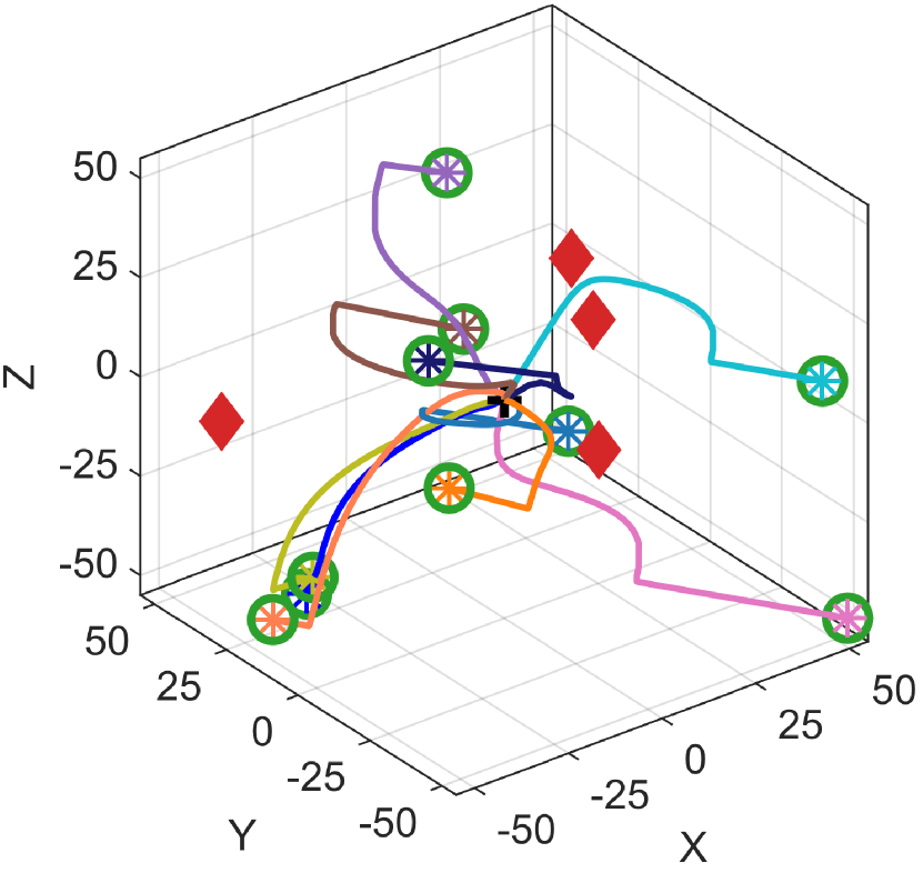
(a) The Richardson Iteration

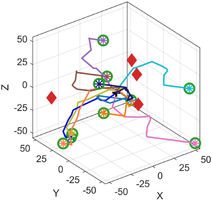
(b) DCG

Figure 3: The convergence trails in $\mathbb{R}^{3}$.

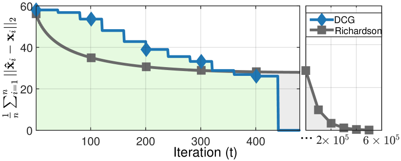
Figure 4: The mean square error w.r.t. iteration rounds.

VI Conclusion

In this paper, we proposed DCG to enable a network of $n$ agents to solve linear equations like $\mathbf{AX=b}$ in fixed rounds of iterations. The DCG algorithm is presented with property analysis and two applications. Compared with traditional Richardson iteration, DCG shows 3 magnitudes faster convergence speed. In future work, we will consider reducing the communication burden that DCG requires.

References

- [1] Shaoshuai Mou, A Stephen Morse, Zhiyun Lin, Lili Wang, and Daniel Fullmer. A distributed algorithm for efficiently solving linear equations. In 2015 54th IEEE Conference on Decision and Control (CDC), pages 6791–6796. IEEE, 2015.
- [2] Y. Diao, Z. Lin, and M. Fu. A barycentric coordinate based distributed localization algorithm for sensor networks. IEEE Transactions on Signal Processing, 62(18):4760–4771, 2014.
- [3] Wolfgang Hackbusch. Iterative Solution of Large Sparse Systems of Equations, chapter 10.2, page 234. Applied Mathematical Sciences. Springer International Publishing, 2 edition, 2016.
- [4] Charu C Aggarwal. Linear Algebra and Optimization for Machine Learning. Springer, 2020.
- [5] Richard Barrett, Michael Berry, Tony F Chan, James Demmel, June Donato, Jack Dongarra, Victor Eijkhout, Roldan Pozo, Charles Romine, and Henk Van der Vorst. Templates for the solution of linear systems: building blocks for iterative methods. SIAM, 1994.
- [6] Yousef Saad. Iterative methods for sparse linear systems. SIAM, 2003.
- [7] Leila Ismail and Rajeev Barua. Implementation and performance evaluation of a distributed conjugate gradient method in a cloud computing environment. Software: Practice and Experience, 43(3):281–304, 2013.
- [8] Songcen Xu, Rodrigo C De Lamare, and H Vincent Poor. Distributed estimation over sensor networks based on distributed conjugate gradient strategies. IET Signal Processing, 10(3):291–301, 2016.
- [9] Xu Fang, Xiaolei Li, and Lihua Xie. 3-d distributed localization with mixed local relative measurements. IEEE Transactions on Signal Processing, 68:5869–5881, 2020.
- [10] Thien-Minh Nguyen, Zhirong Qiu, Thien Hoang Nguyen, Muqing Cao, and Lihua Xie. Persistently excited adaptive relative localization and time-varying formation of robot swarms. IEEE Transactions on Robotics, 36(2):553–560, 2020.
- [11] T. Sun, Y. Wang, D. Li, Z. Gu, and J. Xu. Wcs: Weighted component stitching for sparse network localization. IEEE/ACM Transactions on Networking, 26(5):2242–2253, 2018.
- [12] Y. Wang, T. Sun, G. Rao, and D. Li. Formation tracking in sparse airborne networks. IEEE Journal on Selected Areas in Communications, 36(9):2000–2014, 2018.
- [13] H. Ping, Y. Wang, D. Li, and T. Sun. Flipping free conditions and their application in sparse network localization. IEEE Transactions on Mobile Computing, pages 1–1, 2020.
- [14] Haodi Ping, Yongcai Wang, and Deying Li. Hgo: Hierarchical graph optimization for accurate, efficient, and robust network localization. In Proceedings of the 29th International Conference on Computer Communications and Networks, ICCCN, pages 1–9, 2020.
- [15] T. Han, Z. Lin, R. Zheng, Z. Han, and H. Zhang. A barycentric coordinate based approach to three-dimensional distributed localization for wireless sensor networks. In 2017 13th IEEE International Conference on Control Automation (ICCA), pages 600–605, 2017.