Stars disformally coupled to a shift-symmetric scalar field

Abstract

We investigate static and spherically symmetric stars disformally coupled to a scalar field. The scalar field is assumed to be shift symmetric, and hence the conformal and disformal factors of the metric coupled to matter are dependent only on the kinetic term of the scalar field. Assuming that the scalar field is linearly dependent on time, we consider a general shift-symmetric scalar-tensor theory and a general form of the matter energy-momentum tensor that allows for the anisotropic pressure and the heat flux in the radial direction. This is a natural starting point in light of how the gravitational field equations and the energy-momentum tensor transform under a disformal transformation. By inspecting the structure of the hydrostatic equilibrium equation in the presence of the derivative-dependent conformal and disformal factors, we show that the energy density and tangential pressure must vanish at the surface of a star. This fact is used to prove the disformal invariance of the surface of a star, which was previously subtle and unclear. We then focus on the shift-symmetric k-essence disformally coupled to matter, and study the interior and exterior metric functions and scalar-field profile in more detail. It is found that there are two branches of the solution depending on the velocity of the scalar field. The disformally-related metric functions of the exterior spacetime are also discussed.

I Introduction

The accelerated expansion of the present Universe is implied by the observations of Type Ia supernovae [1, 2]. The source of this accelerated expansion, however, remains unknown and is called generically dark energy. The intriguing question here is whether the dark energy component is in fact just a cosmological constant or some dynamical fields (see, e.g., Ref. [3] for a review). In many models, dark energy is assumed to be described by a scalar field, and the simplest examples include quintessence [4, 5, 6, 7, 8] and k-essence [9, 10]. If the accelerated expansion were caused by such a dynamical scalar field, it might be coupled to (a part of) matter fields, giving rise to signatures of the fifth force. For example, matter may be coupled to a dark energy scalar field $\phi$ through the metric $\widetilde{g}_{\mu\nu}$ which is conformally related to the Einstein-frame metric $g_{\mu\nu}$ as $\widetilde{g}_{\mu\nu}=\Omega(\phi)g_{\mu\nu}$, where the conformal factor $\Omega$ is a function of $\phi$. A more general way of non-minimal coupling is obtained from a disformally related metric [11],

$$\widetilde{g}_{\mu\nu}=\Omega(\phi,X)g_{\mu\nu}+\Gamma(\phi,X)\phi_{\mu}\phi_{\nu},$$ (1)

where $\phi_{\mu}:=\partial_{\mu}\phi$ and the conformal and disformal factors $\Omega$ and $\Gamma$ may depend on $X:=-g^{\mu\nu}\phi_{\mu}\phi_{\nu}/2$ as well as $\phi$. This coupling stems from the most general metric transformation that includes up to first-order derivatives of a scalar field.

Another widely studied approach to account for the accelerated expansion of the Universe is modifying gravity on cosmological scales. Many modified gravity theories can be described by scalar-tensor theories at least effectively in a certain limit. A scalar-field theory for dark energy in the presence of disformally coupled matter can be recast into a scalar-tensor theory minimally coupled to matter through a disformal transformation (1). Conversely, one can perform a transformation (1) to rewrite a given scalar-tensor theory to a scalar-field model of dark energy or another scalar-tensor theory. It is just a matter of the frames as long as the transformation is invertible.

Among various theories, scalar-tensor theories in the Horndeski family [12, 13, 14] have the healthy property that the field equations are of second order and hence the Ostrogradsky instability can be avoided [15, 16, 17]. Recently, more general healthy scalar-tensor theories have been developed named degenerate higher-order scalar-tensor (DHOST) theories [18, 19, 20, 21] (see Refs. [22, 23] for a review). The field equations in DHOST theories are of higher order, but there appear no dangerous Ostrogradsky modes thanks to the degenerate nature of the system. The disformal transformation of the metric plays an important role in DHOST theories: each subclass of DHOST theories is stable under transformations of the form (1), and, in particular, the Lagrangian in the physically interesting subclass called the “class Ia” can always be transformed to the one in the Horndeski family via a disformal transformation [20, 25]. Therefore, a DHOST theory with minimally coupled matter can be mapped to a Horndeski theory with disformally coupled matter. In vacuum, disformal transformations can be used as a solution-generating method for finding new solutions in DHOST theories [27, 28, 29, 30, 31, 32].

Given the importance of the disformal metric in dark energy and modified gravity models, it is natural to explore cosmological and astrophysical implications of disformal coupling to matter. The disformal coupling has been studied in the context of cosmology in Refs. [33, 34, 35, 36, 37, 38, 39, 40, 41, 42, 43, 44]. The invariance of cosmological observables under disformal transformations has been discussed in Refs. [45, 46, 47, 48, 49]. Disformal couplings to baryons and photons have been considered in Refs. [33, 50, 51, 52, 53, 54], while couplings to the dark sector have been studied in Refs. [55, 56]. Other applications can be found in Refs. [57, 58, 59, 60, 61, 62, 63, 64, 65]. A multi-field extension of disformal transformations has been explored in Ref. [66].

In this paper, we study static and spherically symmetric objects in the presence of matter disformally coupled to a scalar field. Relativistic stars in the presence of disformal coupling have been studied in Ref. [67], where the two coupling functions depend only on $\phi$ and not on $X$. Very recently, properties of neutron stars in the presence of $X$-dependent conformal coupling have been discussed [68]. Disformal transformations of various quantities concerning relativistic stars have been investigated in Ref. [69]. Our basic motivation is the same as these works. In contrast to the above works, however, we assume the shift symmetry, $\phi\to\phi+c$ ($c=\,$const.), so that the conformal and disformal factors as well as the gravitational sector of the theory depend on the scalar field only through its derivatives. Under this assumption we consider the linearly time-dependent ansatz for the scalar field. Our setup is similar to, but different from “derivative chameleons” [70] in various aspects. In the latter half of the paper, we focus on a k-essence field disformally coupled to matter. By making a disformal transformation, our system is mapped to a certain DHOST theory in the presence of minimally coupled matter. A distinct point is that the Vainshtein screening mechanism is not expected to operate in that particular DHOST theory, as opposed to the case of generic DHOST theories [71, 72, 73, 74, 75, 76, 77, 78, 79, 80, 81].

This paper is organized as follows. In the next section, we overview the gravitational field equations and fluid equations for a static and spherically symmetric object disformally coupled to a shift-symmetric scalar field. We investigate the hydrostatic equilibrium equation in more detail and show that, in contrast to the case of minimal coupling, the density and tangential pressure must be continuous across the surface of a star. This is the key to prove the disformal invariance of the stellar surface. In Sec. III, we focus on the shift-symmetric k-essence theory disformally coupled to matter and study the interior and exterior solutions of a spherical object. Finally, we draw our conclusions in Sec. IV.

II Spherically symmetric stars disformally coupled to a scalar field

In this section, we first derive general field equations in the case where a scalar field is disformally coupled to matter, and then provide basic equations for the study of spherically symmetric stars in the presence of a disformally coupled scalar field with shift symmetry.

II.1 Field equations

We start with a general class of scalar-tensor theories described by the action

$$S =S_{\rm grav}[g_{\mu\nu},\phi]+S_{\rm m}[\widetilde{g}_{\mu\nu},\psi_{\rm m}]$$

$$=\int{\rm d}^{4}x\sqrt{-g}{\cal L}_{\rm grav}(g_{\mu\nu},\phi)+\int{\rm d}^{4}x\sqrt{-\widetilde{g}}{\cal L}_{\rm m}(\widetilde{g}_{\mu\nu},\psi_{\rm m}).$$ (2)

where the matter field $\psi_{\rm m}$ is coupled to the disformally-related metric (1).

Varying the action (2) with respect to the metric $g_{\mu\nu}$, we obtain the gravitational field equations,

$$\mathcal{E}^{\mu\nu}:=\mathcal{G}^{\mu\nu}-T^{\mu\nu}=0,$$ (3)

where

$$\mathcal{G}^{\mu\nu}=-\frac{2}{\sqrt{-g}}\frac{\delta S_{\rm grav}}{\delta g_{\mu\nu}},\quad T^{\mu\nu}=\frac{2}{\sqrt{-g}}\frac{\delta S_{\rm m}}{\delta g_{\mu\nu}}.$$ (4)

Varying the action (2) with respect to the scalar field $\phi$, we obtain the scalar-field equation of motion,

$$\mathcal{E}_{\phi}:=\mathcal{F}_{\phi}-T_{\phi}=0,$$ (5)

where

$$\mathcal{F}_{\phi}=\frac{1}{\sqrt{-g}}\frac{\delta S_{\rm grav}}{\delta\phi},\quad T_{\phi}=-\frac{1}{\sqrt{-g}}\frac{\delta S_{\rm m}}{\delta\phi}.$$ (6)

We assume that $S_{\rm grav}$ and $S_{\rm m}$ are separately invariant under an infinitesimal coordinate transformation, $x^{\mu}\to x^{\mu}+\xi^{\mu}$. It then follows the Bianchi identities,

$$\nabla_{\nu}{\cal E}^{\mu\nu}+{\cal E}_{\phi}\phi^{\mu} =0,$$ (7)

$$\nabla_{\nu}T^{\mu\nu}+T_{\phi}\phi^{\mu} =0.$$ (8)

Equivalently, one may use $\nabla_{\nu}{\cal G}^{\mu\nu}+{\cal F}_{\phi}\phi^{\mu}=0$ instead of Eq. (7).

Using the fact that $S_{\rm m}$ depends on $g_{\mu\nu}$ and $\phi$ through the disformally-related metric (1), we write $T_{\phi}$ in a more explicit form:

$$T_{\phi}=\nabla_{\mu}W^{\mu}-Z,$$ (9)

where

$$W^{\mu} =w_{1}T^{\mu\nu}\phi_{\nu}+w_{2}T\phi^{\mu}+w_{3}T^{\alpha\beta}\phi_{\alpha}\phi_{\beta}\phi^{\mu},$$ (10)

$$Z =z_{1}T+z_{2}T^{\alpha\beta}\phi_{\alpha}\phi_{\beta},$$ (11)

and $T=T_{\mu}^{\mu}$, with $w_{i}$ and $z_{j}$ being functions of $\phi$ and $X$ defined as

$$w_{1} =\frac{\Gamma}{\Omega},$$ (12)

$$w_{2} =-\frac{1}{2}\frac{\Omega_{X}}{\Omega}\frac{\Omega-2X\Gamma}{\Omega-X\Omega_{X}+2X^{2}\Gamma_{X}},$$ (13)

$$w_{3} =-\frac{1}{2}\frac{\Gamma_{X}}{\Omega}\frac{\Omega-2X\Gamma}{\Omega-X\Omega_{X}+2X^{2}\Gamma_{X}},$$ (14)

$$z_{1} =\frac{1}{2}\left(\frac{\Omega_{\phi}}{\Omega}+\frac{X\Omega_{X}}{\Omega}\frac{\Omega_{\phi}-2X\Gamma_{\phi}}{\Omega-X\Omega_{X}+2X^{2}\Gamma_{X}}\right),$$ (15)

$$z_{2} =\frac{1}{2}\left(\frac{\Gamma_{\phi}}{\Omega}+\frac{X\Gamma_{X}}{\Omega}\frac{\Omega_{\phi}-2X\Gamma_{\phi}}{\Omega-X\Omega_{X}+2X^{2}\Gamma_{X}}\right).$$ (16)

A detailed derivation is presented in Appendix A (see also Ref. [56]). Note that if the coupling functions $\Omega$ and $\Gamma$ preserve the shift symmetry, $\phi\to\phi+c$, then one has $Z=0$.

II.2 Basic equations for spherically symmetric stars

Hereafter, we focus on shift-symmetric theories, $\phi\to\phi+c$, and require the same symmetry for the coupling functions.

Let us consider a static and spherically symmetric metric,

$${\rm d}s^{2}=-e^{\nu(r)}{\rm d}t^{2}+e^{\lambda(r)}{\rm d}r^{2}+r^{2}\left({\rm d}\theta^{2}+\sin^{2}\theta{\rm d}\varphi^{2}\right).$$ (17)

Even though the metric is assumed to be static, the shift symmetry admits a linearly time-dependent configuration of the scalar field,

$$\phi=\mu t+\psi(r),$$ (18)

where $\mu$ ($\neq 0$) is a constant.

We assume the following general form of the energy-momentum tensor,

$$T^{\mu}_{\nu}=\left(\begin{array}[]{cccc}-\rho(r)&e^{-\nu}\chi(r)&0&0\\ -e^{-\lambda}\chi(r)&P_{r}(r)&0&0\\ 0&0&P_{\perp}(r)&0\\ 0&0&0&P_{\perp}(r)\\ \end{array}\right),$$ (23)

where we allow for the off-diagonal component, $\chi(r):=-T_{tr}$, i.e., the heat flux in the radial direction, and anisotropic pressure, $P_{r}\neq P_{\perp}$. Below we will see that in general this off-diagonal component is necessary if $\mu\neq 0$.

Under the above ansatz, the radial and temporal components of the Bianchi identities (7) read, respectively,

$$\frac{e^{-\nu/2}}{r^{2}}\left(r^{2}e^{\nu/2}{\cal E}_{r}^{r}\right)^{\prime}-\frac{\nu^{\prime}}{2}{\cal E}_{t}^{t}-\frac{2}{r}{\cal E}_{\perp}+{\cal E}_{\phi}\psi^{\prime} =0,$$ (24)

$$\frac{e^{-(\nu+\lambda)/2}}{r^{2}}\left[r^{2}e^{(\nu+\lambda)/2}{\cal E}_{t}^{r}\right]^{\prime}+{\cal E}_{\phi}\mu =0,$$ (25)

where a prime denotes differentiation with respect to $r$ and ${\cal E}_{\perp}$ stands for the angular components, ${\cal E}_{\perp}:={\cal E}_{\theta}^{\theta}={\cal E}_{\varphi}^{\varphi}$. These identities show that one may take

$$\mathcal{E}^{t}_{t}={\cal G}_{t}^{t}+\rho=0,$$ (26)

$$\mathcal{E}^{r}_{r}={\cal G}_{r}^{r}-P_{r}=0,$$ (27)

$$\mathcal{E}_{tr}={\cal G}_{tr}+\chi=0,$$ (28)

as independent equations, while ${\cal E}_{\perp}=0$ and ${\cal E}_{\phi}=0$ follow automatically from the Bianchi identities.

We now look into Eq. (8). Similarly to Eqs. (24) and (25), we obtain

$$P_{r}^{\prime}+\frac{\nu^{\prime}}{2}(\rho+P_{r})+\frac{2}{r}(P_{r}-P_{\perp})+T_{\phi}\psi^{\prime} =0,$$ (29)

$$\frac{e^{-(\nu+\lambda)/2}}{r^{2}}\left[r^{2}e^{(\nu+\lambda)/2}T_{t}^{r}\right]^{\prime}+T_{\phi}\mu =0,$$ (30)

where, by noting that $Z=0$ due to the shift symmetry,

$$T_{\phi}=\frac{e^{-(\nu+\lambda)/2}}{r^{2}}\left[r^{2}e^{(\nu+\lambda)/2}W^{r}\right]^{\prime}.$$ (31)

Explicitly, one has

$$W^{r} =e^{-\lambda}\psi^{\prime}\bigl{\{}w_{1}P_{r}-w_{2}(\rho-P_{r}-2P_{\perp})$$

$$\quad+w_{3}\left[\mu^{2}e^{-\nu}\rho+e^{-\lambda}(\psi^{\prime})^{2}P_{r}\right]\bigr{\}}$$

$$\quad+\mu e^{-\nu-\lambda}\left[w_{1}+2w_{3}e^{-\lambda}(\psi^{\prime})^{2}\right]\chi.$$ (32)

One can immediately integrate Eq. (30) to get

$$e^{-\lambda}\chi-\mu W^{r}=\frac{{\cal C}e^{-(\nu+\lambda)/2}}{r^{2}},$$ (33)

where ${\cal C}$ is an integration constant. To fix ${\cal C}$, let us consider the behavior of the left-hand side at the center. We may assume that $\nu$, $\lambda$, $\psi^{\prime}$, $\rho$, $P_{r}$, $P_{\perp}$, and $\chi$ do not diverge as $r\to 0$. Then, $W^{r}$ does not diverge at the center. This observation leads us to set ${\cal C}=0$. Having shown that, we can solve Eq. (33) for $\chi$ to obtain

$$\chi=\mu\psi^{\prime}h(\nu,\lambda,\psi^{\prime},\rho,P_{r},P_{\perp}),$$ (34)

where

$$h :=\frac{w_{1}P_{r}-w_{2}(\rho-P_{r}-2P_{\perp})}{1-\mu^{2}e^{-\nu}[w_{1}+2w_{3}e^{-\lambda}(\psi^{\prime})^{2}]}$$

$$\quad+\frac{w_{3}\left[\mu^{2}e^{-\nu}\rho+e^{-\lambda}(\psi^{\prime})^{2}P_{r}\right]}{1-\mu^{2}e^{-\nu}[w_{1}+2w_{3}e^{-\lambda}(\psi^{\prime})^{2}]}.$$ (35)

In general, there is no reason to impose $h=0$ and hence we have $\chi\neq 0$.

II.3 The surface of a star

We now consider more specifically the case where ${\cal L}_{\rm grav}$ is given by that of the shift-symmetric Horndeski theory,

$${\cal L}_{\rm grav} =G_{2}(X)-G_{3}(X)\Box\phi+G_{4}(X)R$$

$$\quad+G_{4X}\left[(\Box\phi)^{2}-\nabla_{\mu}\nabla_{\nu}\phi\nabla^{\mu}\nabla^{\nu}\phi\right].$$ (36)

We do not consider the “$G_{5}$” terms for simplicity; they do not lead to no essential difference in the following results.

The goal of this subsection is to discuss the matching conditions at the surface of a star, $r=r_{s}$, defined by $P_{r}(r_{s})=0$. For this purpose only the structure of the highest derivative terms in ${\cal G}_{\mu\nu}$ is important. We have

$${\cal G}_{t}^{t} =g_{1}+g_{2}\lambda^{\prime}+g_{3}\psi^{\prime\prime}=-\rho,$$ (37)

$${\cal G}_{r}^{r} =g_{4}-g_{2}\nu^{\prime}=P_{r},$$ (38)

$${\cal G}_{tr} =\frac{\mu e^{\lambda}}{2}\left(g_{5}+g_{3}\nu^{\prime}\right)=-\chi,$$ (39)

where $g_{a}=g_{a}(\nu,\lambda,\psi^{\prime})$ ($a=1,2,3,4,5$). Using Eqs. (38) and (39) one can eliminate $\nu^{\prime}$ to get the equation of the form

$$\lambda=F_{\lambda}(\nu,\psi^{\prime},P_{r},\chi).$$ (40)

Equation (29) is independent of the specific form of the gravitational part of the Lagrangian.

We impose that the induced metric is continuous across the surface of a star, and hence $\nu$ is continuous. If the matter is minimally coupled to gravity, $\rho$ and $P_{\perp}$ are allowed to be discontinuous at $r=r_{s}$, and then it follows from Eqs. (37) and (40) that $\lambda^{\prime}$ and $\psi^{\prime\prime}$ may be discontinuous. The situation becomes more subtle if the matter is non-minimally coupled to gravity through $X$-dependent $\Omega$ and $\Gamma$. Now, we have

$$T_{\phi}\supset\frac{e^{-\lambda}\psi^{\prime}\left[-(w_{2}-w_{3}\mu^{2}e^{-\nu})\rho^{\prime}+2w_{2}P_{\perp}^{\prime}\right]}{1-\mu^{2}e^{-\nu}[w_{1}+2w_{3}e^{-\lambda}(\psi^{\prime})^{2}]},$$ (41)

which yields the delta functions $\sim\delta(r-r_{s})$. However, we see that no other terms in Eq. (29) contain the delta functions canceling $T_{\phi}$. It is therefore required in the present case that $\rho$ and $P_{\perp}$ are continuous across the surface, i.e., $\lim_{r\to r_{s}-0}\rho(r)=0$ and $\lim_{r\to r_{s}-0}P_{\perp}(r)=0$. Note that the first derivatives of $\rho$, $P_{r}$, and $P_{\perp}$ may be discontinuous at $r=r_{s}$, and so are $\lambda^{\prime}$ and $\psi^{\prime\prime}$, provided that $g_{2}\lambda^{\prime}+g_{3}\psi^{\prime\prime}$ is continuous. Note also that there is an exceptional case where $\psi^{\prime}(r_{s})=0$, to which the above argument does not apply.

The requirement that $\rho(r_{s})=P_{\perp}(r_{s})=0$ in the presence of the $X$-dependent coupling functions has a direct implication on the disformal invariance of the notion of the surface of a star. As discussed in Appendix B, the radial pressure transforms under a disformal transformation as

$$\widetilde{P}_{r}=m_{4}\rho+m_{5}P_{r}+m_{6}P_{\perp},$$ (42)

where the explicit expressions for $m_{4}$, $m_{5}$, and $m_{6}$ can be read off from the equations in Appendix B. It is obvious that if $\rho(r_{s})=P_{r}(r_{s})=P_{\perp}(r_{s})=0$ then $\widetilde{P}_{r}$ vanishes there. Therefore, the notion of the surface of a star is invariant under a disformal transformation. By utilizing the consistency of the hydrostatic equation (29), we have thus arrived at the stronger conclusion than that in Ref. [69]. Note in passing that in the aforementioned exceptional case where $\psi^{\prime}(r_{s})=0$, we have $m_{4}=m_{6}=0$ and hence the same conclusion holds.

III The case of k-essence

Let us study the case in which the gravitational part of the Lagrangian is given by

$${\cal L}_{\rm grav}=\frac{M_{\rm Pl}^{2}}{2}R+G_{2}(X),$$ (43)

i.e., the case of shift-symmetric k-essence disformally coupled to matter. We require that the Minkowski spacetime is a solution of the theory. The function $G_{2}$ then must be such that

$$G_{2}(X_{*})=0,\quad G_{2X}(X_{*})=0,$$ (44)

for some $X_{*}$ (see Eqs. (46)–(48) below). The value of $X_{*}$ is thus determined from the parameters of the model under consideration.

If $\Gamma=0$, the speed of gravitational waves in this theory coincides with that of light. Moreover, the theory is free from graviton decay into dark energy [85, 86] and dark energy instability induced by gravitational waves [87]. Therefore, k-essence with $\Gamma=0$ is consistent with gravitational wave observations [88]. In the following discussion, however, we will not restrict ourselves to the case of $\Gamma=0$ for the sake of generality.

The $(tr)$-component of the gravitational field equations reads

$${\cal G}_{tr}=-\mu\psi^{\prime}G_{2X}=-\chi,$$ (45)

which, combined with Eq. (34), gives

$$\mu\psi^{\prime}(h-G_{2X})=0.$$ (46)

Thus, we have two branches: $\psi^{\prime}=0$ and $h-G_{2X}=0$. We call the former the Branch I and the latter the Branch II. The $(tt)$- and $(rr)$-components are given, respectively, by

$${\cal G}_{t}^{t} =-\frac{M_{\rm Pl}^{2}}{r^{2}}\left(1-e^{-\lambda}+re^{-\lambda}\lambda^{\prime}\right)+2XG_{2X}-G_{2}=-\rho,$$ (47)

$${\cal G}_{r}^{r} =-\frac{M_{\rm Pl}^{2}}{r^{2}}\left(1-e^{-\lambda}-re^{-\lambda}\nu^{\prime}\right)-G_{2}=P_{r}.$$ (48)

Note that in the Branch I there is no effect of the coupling functions $\Omega$ and $\Gamma$ on the profile of the metric functions.

III.1 Interior solution

Let us begin with the inspection of the interior solution. We assume that the radial and tangential pressures are related to $\rho$ through equations of state: $P_{r}=P_{r}(\rho)$ and $P_{\perp}=P_{\perp}(\rho)$. To determine the metric functions in the stellar interior, we first solve Eq. (46) algebraically to write $\psi^{\prime}=F(\nu,\lambda,\rho)$. (Obviously, $F=0$ in the Branch I.) Using this, one can express $T_{\phi}$ in terms of $\nu,\lambda,\rho$, and their first derivatives. Thus eliminating $\psi^{\prime}$, Eqs. (29), (47), and (48) reduce to three first-order differential equations for $\nu$, $\lambda$, and $\rho$. Given the boundary conditions at $r=0$, one can integrate these equations outwards to determine the stellar structure. The radius of a star, $r_{s}$, is defined by $P_{r}(r_{s})=0$.

We require that $\nu$, $\lambda$, $\psi$, $\rho$, $P_{r}$, and $P_{\perp}$ are regular at $r=0$. Then, near the center, we may expanded these quantities as

$$\nu =\nu_{c}+\frac{\nu_{2}}{2}r^{2}+\cdots,$$ (49)

$$\lambda =0+\frac{\lambda_{2}}{2}r^{2}+\cdots,$$ (50)

$$\psi^{\prime} =\psi_{2}r+\dots,$$ (51)

$$\rho =\rho_{c}+\frac{\rho_{2}}{2}r^{2}+\cdots,$$ (52)

$$P_{r} =P_{r,c}+\frac{P_{r,2}}{2}r^{2}+\cdots,$$ (53)

$$P_{\perp} =P_{\perp,c}+\frac{P_{\perp,2}}{2}r^{2}+\cdots.$$ (54)

Note here that, as can be seen from Eqs. (47) and (48), we have $1-e^{-\lambda}={\cal O}(r^{2})$ near the center and hence $\lambda(0)=0$. In contrast, $\nu_{c}$ is not determined locally and one can integrate the equations for any value of $\nu_{c}$. The choice of $\nu_{c}$ is correlated with how one sets the zero of the gravitational potential. Usually, one tunes $\nu_{c}$ so that the boundary conditions in the stellar exterior are satisfied.

From Eqs. (49)–(51) we see that

$$X=X_{c}-\frac{1}{2}(X_{c}\nu_{2}+\psi_{2}^{2})r^{2}+\cdots,$$ (55)

where

$$X_{c}:=\frac{1}{2}\mu^{2}e^{-\nu_{c}}.$$ (56)

Therefore, for a function $f$ of $X$ (such as $w_{1}$), we have $f(X)=f(X_{c})+{\cal O}(r^{2})$ near the center. Now, it is easy to see that $W^{r}={\cal O}(r)$ and $T_{\phi}=\;$constant near the center. This fact and Eq. (29) imply that

$$P_{r}-P_{\perp}={\cal O}(r^{2})\quad\Rightarrow\quad P_{r,c}=P_{\perp,c}\,(=:P_{c}).$$ (57)

On the basis of the above argument, let us turn back to Eq. (46). It is clear that the Branch I is always consistent with the boundary conditions at $r=0$. In particular, in this branch, $\mu$ is a free parameter as far as the interior solution is concerned. In contrast, for a given central density $\rho_{c}$ (and a central pressure according to the equation of state),

$$\left.h-G_{2X}\right|_{r=0} =\frac{w_{1}P_{c}-w_{2}(\rho_{c}-3P_{c})+2X_{c}w_{3}\rho_{c}}{1-2X_{c}w_{1}}$$

$$\quad-G_{2X}(X_{c})$$ (58)

is vanishing only if a particular value of $X_{c}$ is chosen. This implies that the Branch II is consistent only for a particular value of $\mu$, and this particular value is dependent on the central density $\rho_{c}$ of a star.

III.2 Exterior solution

First let us consider the Branch I, in which the interior solution with $\psi^{\prime}=0$ is smoothly connected to the exterior solution with $\psi^{\prime}=0$. In this branch one cannot obtain an analytic solution valid in the entire region of the stellar exterior. We therefore discuss linearized solutions around the Minkowski spacetime with $X=X_{*}$:

$$\nu \simeq\nu_{*}+\delta\nu(r)\ll 1,\quad\lambda\simeq\delta\lambda(r)\ll 1,$$

$$X \simeq\frac{\mu^{2}}{2}e^{-\nu_{*}}(1-\delta\nu),$$ (59)

where

$$\nu_{*}=\ln\left(\frac{\mu^{2}}{2X_{*}}\right).$$ (60)

By taking $\mu=\sqrt{2X_{*}}$, one can set $\nu_{*}=0$. With this choice, $\mu$ is determined solely by theory parameters.

Linearization is justified sufficiently away from the star, $r\gg r_{s}$. The linearized field equations read

$$\frac{r\delta\lambda^{\prime}+\delta\lambda}{r^{2}}+q\delta\nu=0,\quad r\delta\nu^{\prime}-\delta\lambda=0,$$ (61)

where we defined

$$q:=\frac{2X_{*}^{2}G_{2XX}\left(X_{*}\right)}{M_{\mathrm{Pl}}^{2}}.$$ (62)

The general solution to these equations is given by

$$\delta\nu =C_{1}\frac{\cos(\sqrt{q}r)}{r}+C_{2}\frac{\sin(\sqrt{q}r)}{r},$$ (63)

$$\delta\lambda =-\sqrt{q}\left[C_{1}\sin(\sqrt{q}r)-C_{2}\cos(\sqrt{q}r)\right]-\delta\nu,$$ (64)

for $q>0$ and

$$\delta\nu =C_{3}\frac{e^{\sqrt{-q}r}}{r}+C_{4}\frac{e^{-\sqrt{-q}r}}{r},$$ (65)

$$\delta\lambda =\sqrt{-q}\left[C_{3}e^{\sqrt{-q}r}-C_{4}e^{-\sqrt{-q}r}\right]-\delta\nu,$$ (66)

for $q<0$.

The oscillatory behavior for $q>0$ is qualitatively similar to what has been found in the Newtonian potential in the ghost condensate model [89]. Suppose that the length scale associated to $q$ is very large, say, the cosmological horizon scale, and consider the metric in the region $r_{s}\ll r\ll 1/\sqrt{q}$. We then have

$$\delta\nu\simeq C_{2}\sqrt{q}+\frac{C_{1}}{r},\quad\delta\lambda\simeq-\frac{C_{1}}{r}.$$ (67)

After fixing $\mu$ as $\mu=\sqrt{2X_{*}}$, one can tune $\nu_{c}$ so that the boundary condition $C_{2}=0$ is satisfied. The metric functions for $r_{s}\ll r\ll 1/\sqrt{q}$ are thus described by the linearized Schwarzschild solution with $-C_{1}$ being the mass parameter.

In the case of $q<0$, the diverging term can be removed by imposing the boundary condition $C_{3}=0$. After fixing $\mu$ as $\mu=\sqrt{2X_{*}}$, this can be satisfied by tuning $\nu_{c}$. Then, in the region $r_{s}\ll r\ll 1/\sqrt{-q}$, we have

$$\delta\nu\simeq-C_{4}\sqrt{-q}+\frac{C_{4}}{r},\quad\delta\lambda\simeq-\frac{C_{4}}{r}.$$ (68)

In this case one can no longer remove the constant part $-C_{4}\sqrt{-q}$, but this term is physically unimportant.

Next, let us consider the Branch II, in which the interior solution with $h-G_{2X}=0$ is connected to the exterior solution with $G_{2X}=0$ at the surface where $h=0$. In this branch, we have $X=X_{*}$ in the entire region of the stellar exterior, and the metric functions take the Schwarzschild form,

$$e^{\nu}=e^{\nu_{\infty}}\left(1-\frac{C_{0}}{r}\right),\quad e^{-\lambda}=1-\frac{C_{0}}{r},$$ (69)

where $\nu_{\infty}$ and $C_{0}$ are integration constants. Note that $\nu_{\infty}$ has no physical significance and can be set to zero by shifting $\nu_{c}$.

III.3 Numerical examples

As a concrete example we consider a specific model with

$$G_{2}=\frac{qM_{\rm Pl}^{2}}{4}\frac{(X-X_{*})^{2}}{X_{*}^{2}},\quad\Omega=e^{2\beta X/X_{*}},\quad\Gamma=0,$$ (70)

and present our numerical results in Figs. 1–4. We assume for simplicity that the equation of state is isotropic and is given by $P_{r}=P_{\perp}\propto\rho^{2}$, where the constant of proportionality is fixed so that $P_{c}=0.1\rho_{c}$. We use units where $\rho_{c}/M_{\rm Pl}^{2}=1$. The parameters are given by $q=0.01$ for the solutions in Figs 1 and 2, $q=-0.01$ in Fig. 3, and $q=\beta=0.01$ in Fig. 4.

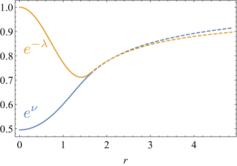
Figure 1: The metric functions in the case where $q>0$ and $\mu=\sqrt{2X_{*}}$. The interior (exterior) region corresponds to solid (dashed) lines. The $r\lesssim 1/\sqrt{q}$ region is zoomed.

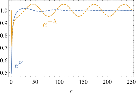
Figure 2: The same as Fig. 1, but the plotted range is $r\gg 1/\sqrt{q}$ so that the oscillatory behavior can be seen. The numerical solution is well approximated by $\nu\simeq-0.49\cos(\sqrt{q}r)/r$ for $r\gtrsim 1/\sqrt{q}$.

Figure 3: The metric functions in the case where $q<0$ and $\mu=\sqrt{2X_{*}}$. The interior (exterior) region corresponds to solid (dashed) lines. The numerical solution is well approximated by $\nu\simeq-0.43e^{-\sqrt{-q}r}/r$ for $r\gtrsim 1/\sqrt{-q}$.

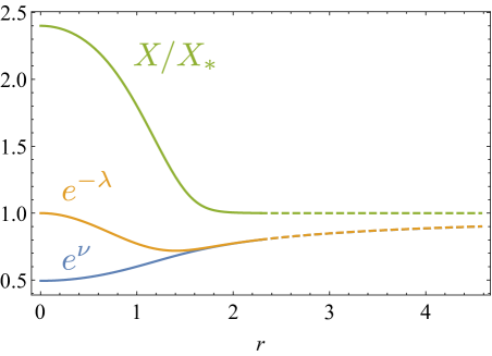
Figure 4: The metric functions and $X/X_{*}$ in the case where $\mu$ is chosen so that $h-G_{2X}=0$ at the center. The interior (exterior) region corresponds to solid (dashed) lines.

The Branch I solution with $q>0$ is shown in Figs. 1 and 2, where the behavior described in the previous subsection can be seen. Similarly, the Branch I solution with $q<0$ is presented in Fig. 3. Figure 4 shows the numerical example of the Branch II. The interior solution is smoothly matched to the exterior stealth Schwarzschild solution.

III.4 Gravity that matter feels

We have thus obtained the profile of the metric functions $\nu$ and $\lambda$. However, since matter is coupled to the disformally-related metric $\widetilde{g}_{\mu\nu}$, the actual metric that we observe is $\widetilde{g}_{\mu\nu}$. Therefore, let us write the line element $\widetilde{{\rm d}s}{}^{2}=\widetilde{g}_{\mu\nu}{\rm d}\widetilde{x}^{\mu}\widetilde{x}^{\nu}$ in the form

$$\widetilde{{\rm d}s}{}^{2} =-(1+2\widetilde{\Phi}){\rm d}\widetilde{\tau}^{2}$$

$$\quad+(1-2\widetilde{\Psi})[{\rm d}\widetilde{\varrho}^{2}+\widetilde{\varrho}^{2}({\rm d}\theta^{2}+\sin^{2}\theta{\rm d}\varphi^{2})],$$ (71)

and evaluate $\widetilde{\Phi}$ and $\widetilde{\Psi}$ in the region where linearization is valid.

In the Branch I, we have $X\simeq X_{*}(1-\delta\nu)$ and hence $\Omega(X)=\Omega_{*}-X_{*}\Omega_{X*}\delta\nu$, where the quantities with the asterisk are evaluated at $X=X_{*}$. By performing the coordinate transformation

$$\widetilde{\tau} =(\Omega_{*}-2X_{*}\Gamma_{*})^{1/2}t,$$ (72)

$$\widetilde{\varrho} =\Omega^{1/2}_{*}\left(1+\frac{1}{2}\int^{r}\frac{\delta\lambda}{r^{\prime}}{\rm d}r^{\prime}\right)r,$$ (73)

we can recast the disformally-related metric to the form of Eq. (71) and find that

$$\widetilde{\Phi} =\frac{\Omega_{*}-X_{*}(\Omega_{X*}-2X_{*}\Gamma_{X*})}{2(\Omega_{*}-2X_{*}\Gamma_{*})}\delta\nu,$$ (74)

$$\widetilde{\Psi} =\frac{1}{2}\int^{r}\frac{\delta\lambda}{r^{\prime}}{\rm d}r^{\prime}+\frac{X_{*}\Omega_{X*}}{2\Omega_{*}}\delta\nu$$

$$=\frac{1}{2}\left(1+\frac{X_{*}\Omega_{X*}}{\Omega_{*}}\right)\delta\nu,$$ (75)

where we used $\delta\lambda=r\delta\nu^{\prime}$ in the last line. We therefore have

$$\frac{\widetilde{\Psi}}{\widetilde{\Phi}}=\frac{(1+X_{*}\Omega_{X*}/\Omega_{*})(1-2X_{*}\Gamma_{*}/\Omega_{*})}{1-X_{*}(\Omega_{X*}-2X_{*}\Gamma_{X*})/\Omega_{*}}.$$ (76)

This result can be used to evaluate the deviation from general relativity. Note that it is easy to find the cases where $\Omega_{X}$ and $\Gamma$ are not small, but $\widetilde{\Psi}\simeq\widetilde{\Phi}$. A simple example is given by

$$\Omega=\Omega_{0}e^{\beta_{1}X/X_{*}},\quad\Gamma=\frac{\beta_{2}\Omega_{0}}{X_{*}}e^{\beta_{1}X/X_{*}}.$$ (77)

In this case we see that $\widetilde{\Psi}\simeq\widetilde{\Phi}$ for $\beta_{2}\simeq\beta_{1}/(1+2\beta_{1})$. However, in the case of conformal coupling, $\Gamma=0$, $X_{*}\Omega_{X*}/\Omega$ must be sufficiently small.

In the Branch II, the disformally-related metric cannot take the form of Eq. (71) in general. Instead one needs to consider the metric with a solid deficit angle [27],

$$\widetilde{{\rm d}s}{}^{2} =-(1+2\widetilde{\Phi}){\rm d}\widetilde{\tau}^{2}$$

$$\quad+(1-2\widetilde{\Psi})[{\rm d}\widetilde{\varrho}^{2}+s_{0}^{-1}\widetilde{\varrho}^{2}({\rm d}\theta^{2}+\sin^{2}\theta{\rm d}\varphi^{2})],$$ (78)

where $s_{0}$ is a constant. To put the metric into this form, we perform the coordinate transformation

$${\rm d}\widetilde{\tau} =(\Omega_{*}-\mu^{2}\Gamma_{*})\left({\rm d}t-\frac{\mu\Gamma\psi^{\prime}}{\Omega e^{\nu}-\mu^{2}\Gamma}{\rm d}r\right),$$ (79)

$$\widetilde{\varrho} =s_{0}^{1/2}\Omega_{*}^{1/2}\left[1+\frac{1}{2}\int^{r}\left(\frac{\delta\lambda}{r^{\prime}}-\frac{\mu^{2}\Gamma_{*}}{\Omega_{*}-\mu^{2}\Gamma_{*}}\frac{\delta\nu}{r^{\prime}}\right){\rm d}r^{\prime}\right]r,$$ (80)

where

$$s_{0}:=\frac{\Omega_{*}-2X_{*}\Gamma_{*}}{\Omega_{*}-\mu^{2}\Gamma_{*}}.$$ (81)

It is then found that

$$\widetilde{\Phi} =\frac{1}{2}\frac{\Omega_{*}}{\Omega_{*}-\mu^{2}\Gamma_{*}}\delta\nu,$$ (82)

$$\widetilde{\Psi} =\frac{1}{2}\int^{r}\left(\frac{\delta\lambda}{r^{\prime}}-\frac{\mu^{2}\Gamma_{*}}{\Omega_{*}-\mu^{2}\Gamma_{*}}\frac{\delta\nu}{r^{\prime}}\right){\rm d}r^{\prime}.$$ (83)

Since $\delta\nu=-\delta\lambda=-C_{0}/r$, we have

$$\widetilde{\Phi}=\widetilde{\Psi}\propto\frac{1}{\widetilde{\varrho}}.$$ (84)

Thus, in the Branch II the difference from general relativity can be found in the solid deficit angle [27]. Since the deficit angle changes geodesics, we can measure its effect by observing the light propagation, e.g., the deflection angle of the light. [90, 91].

IV Conclusions

In this paper, we have studied static and spherically symmetric stars disformally coupled with a scalar field. We have been focusing on shift-symmetric theories, so that the conformal and disformal factors of the metric that couples to matter are dependent only on $X:=-g^{\mu\nu}\partial_{\mu}\phi\partial_{\nu}\phi/2$. The shift symmetry admits the scalar-field configuration that is dependent linearly on time, $\phi=\mu t+\psi(r)$, where $\mu\,(=\partial_{t}\phi)$ is the constant velocity of the scalar field. Starting from a general scalar-tensor theory and a general form of the energy-momentum tensor, we have overviewed the gravitational field equations and fluid equations for matter. More specifically, our energy-momentum tensor allows for the radial heat flux and anisotropic pressure. Such a general form of the energy-momentum tensor is implied by the way it transforms under a disformal transformation, and hence is natural to consider in the present setup.

We have investigated the density and pressure profile in the vicinity of the surface of a star (defined as the location at which the radial pressure vanishes, $P_{r}(r_{s})=0$). It is known that the density $\rho$ and tangential pressure $P_{\perp}$ may be discontinuous across the stellar surface as long as matter is minimally coupled to gravity. In the presence of $X$-dependent conformal and disformal factors, however, we have shown that $\rho(r_{s})=P_{\perp}(r_{s})=0$ is requried by the structure of the hydrostatic equilibrium equation. This in turn indicates the disformal invariance of the surface of a star. This fact was previously subtle and shown only when certain extra conditions are met [69].

We have then concentrated on the shift-symmetric k-essence theory disformally coupled to matter, and studied the interior and exterior metric functions and scalar-field profile. We have found that there are two branches of the solution depending on the value of $\mu$. One branch, which we call the Branch I, is characterized by the trivial scalar-field profile, $\psi^{\prime}=0$. The velocity $\mu$ in the Branch I is determined solely by theory parameters. The other branch, which we call the Branch II, is characterized by the stealth Schwarzschild geometry with the constant $X$ profile in the exterior region. The velocity $\mu$ in the Branch II is determined by the central density as well as theory parameters. The disformally transformed metric that couples to matter has also been discussed. We have found in particular that in the Branch I the standard result of general relativity can be reproduced if a certain relation between the conformal and disformal factors is satisfied.

As we have seen in Fig. 2, the Branch I solution exhibits an oscillatory behavior of the metric functions far away from the source, which may lead to interesting cosmological consequences. We hope to come back to the study of cosmology in the present setup in the near future.

Appendix A Derivation of Eqs. (9)–(16)

We start with writing $T^{\mu\nu}$ as

$$T^{\mu\nu} =\frac{\partial\widetilde{g}_{\alpha\beta}}{\partial g_{\mu\nu}}\cdot\frac{2}{\sqrt{-g}}\frac{\partial}{\partial\widetilde{g}_{\alpha\beta}}\left(\sqrt{-\widetilde{g}}{\cal L}_{\rm m}\right)$$

$$={\cal J}_{g}\biggl{(}\Omega\widetilde{T}^{\mu\nu}+\frac{1}{2}\Omega_{X}\phi^{\mu}\phi^{\nu}g_{\alpha\beta}\widetilde{T}^{\alpha\beta}$$

$$\quad+\frac{1}{2}\Gamma_{X}\phi^{\mu}\phi^{\nu}\phi_{\alpha}\phi_{\beta}\widetilde{T}^{\alpha\beta}\biggr{)},$$ (85)

where

$${\cal J}_{g} =\frac{\sqrt{-\widetilde{g}}}{\sqrt{-g}}=\Omega^{3/2}\sqrt{\Omega-2X\Gamma},$$ (86)

$$\widetilde{T}^{\mu\nu} =\frac{2}{\sqrt{-\widetilde{g}}}\frac{\partial}{\partial\widetilde{g}_{\mu\nu}}\left(\sqrt{-\widetilde{g}}{\cal L}_{\rm m}\right).$$ (87)

By contracting Eq. (85) with $g_{\mu\nu}$ and $\phi_{\mu}\phi_{\nu}$ and solving the resultant equations for $g_{\mu\nu}\widetilde{T}^{\mu\nu}$ and $\phi_{\mu}\phi_{\nu}\widetilde{T}^{\mu\nu}$, we obtain

$$g_{\mu\nu}\widetilde{T}^{\mu\nu} =\frac{(\Omega+2X^{2}\Gamma_{X})T+X\Gamma_{X}\phi_{\mu}\phi_{\nu}T^{\mu\nu}}{{\cal J}_{g}\Omega(\Omega-X\Omega_{X}+2X^{2}\Gamma_{X})},$$ (88)

$$\phi_{\mu}\phi_{\nu}\widetilde{T}^{\mu\nu} =\frac{-2X^{2}\Omega_{X}T+(\Omega-X\Omega_{X})\phi_{\mu}\phi_{\nu}T^{\mu\nu}}{{\cal J}_{g}\Omega(\Omega-X\Omega_{X}+2X^{2}\Gamma_{X})}.$$ (89)

Thus, we have

$${\cal J}_{g}\Omega\widetilde{T}^{\mu\nu} =T^{\mu\nu}-\frac{\Omega_{X}\phi^{\mu}\phi^{\nu}T}{2(\Omega-X\Omega_{X}+2X^{2}\Gamma_{X})}$$

$$\quad-\frac{\Gamma_{X}\phi^{\mu}\phi^{\nu}T^{\alpha\beta}\phi_{\alpha}\phi_{\beta}}{2(\Omega-X\Omega_{X}+2X^{2}\Gamma_{X})}.$$ (90)

Now, we may write

$$T_{\phi}=-\frac{1}{\sqrt{-g}}\frac{\delta S_{\phi}}{\delta\phi}=\nabla_{\mu}W^{\mu}-Z,$$ (91)

where

$$W^{\mu} =\frac{1}{\sqrt{-g}}\frac{\partial}{\partial\phi_{\mu}}\left(\sqrt{-\widetilde{g}}{\cal L}_{\rm m}\right)=\frac{1}{2}\frac{\partial\widetilde{g}_{\alpha\beta}}{\partial\phi_{\mu}}\cdot{\cal J}_{g}\widetilde{T}^{\alpha\beta},$$ (92)

$$Z =\frac{1}{\sqrt{-g}}\frac{\partial}{\partial\phi}\left(\sqrt{-\widetilde{g}}{\cal L}_{\rm m}\right)=\frac{1}{2}\frac{\partial\widetilde{g}_{\alpha\beta}}{\partial\phi}\cdot{\cal J}_{g}\widetilde{T}^{\alpha\beta}.$$ (93)

Substituting Eq. (90) to Eqs. (92) and (93), we arrive at Eqs. (10)–(16).

Appendix B Disformal transformation of the energy-momentum tensor

Here we summarize the disformal transformation of each component of the energy-momentum tensor that composes a star. One can find a similar discussion for a slowly rotating star dressed with a time-independent scalar field in Ref. [69].

For a static and spherically symmetric metric, Eq. (1) reads

$$\widetilde{g}_{\mu\nu}{\rm d}x^{\mu}{\rm d}x^{\nu} =-\left(\Omega e^{\nu}-\mu^{2}\Gamma\right){\rm d}t^{2}+2\mu\Gamma\psi^{\prime}{\rm d}t{\rm d}r$$

$$\quad+\left[\Omega e^{\lambda}+\Gamma(\psi^{\prime})^{2}\right]{\rm d}r^{2}$$

$$\quad+\Omega r^{2}\left({\rm d}\theta^{2}+\sin^{2}\theta{\rm d}\varphi^{2}\right).$$ (94)

Introducing the new coordinates defined by

$${\rm d}\widetilde{t} ={\rm d}t-\frac{\mu\Gamma\psi^{\prime}}{\Omega e^{\nu}-\mu^{2}\Gamma}{\rm d}r,$$ (95)

$$\widetilde{r} =\Omega^{1/2}r,$$ (96)

the metric can then be put into the standard diagonal form as

$$\widetilde{g}_{\mu\nu}{\rm d}\widetilde{x}^{\mu}{\rm d}\widetilde{x}^{\nu} =-e^{\widetilde{\nu}}{\rm d}\widetilde{t}^{2}+e^{\widetilde{\lambda}}{\rm d}\widetilde{r}^{2}+\widetilde{r}^{2}\left({\rm d}\theta^{2}+\sin^{2}\theta{\rm d}\varphi^{2}\right),$$ (97)

where

$$e^{\widetilde{\nu}} =\Omega e^{\nu}-\mu^{2}\Gamma,$$ (98)

$$e^{\widetilde{\lambda}} =\frac{\Omega-2X\Gamma}{\Omega-\mu^{2}e^{-\nu}\Gamma}\left(1+\frac{rX^{\prime}\Omega_{X}}{2\Omega}\right)^{-2}e^{\lambda}.$$ (99)

Note that we do not always have $\widetilde{\nu}\to 0$ and $\widetilde{\lambda}\to 0$ as $\widetilde{r}\to\infty$ even if $\nu\to 0$ and $\lambda\to 0$ as $r\to\infty$. One can rescale the coordinates so that $\widetilde{\nu}\to 0$ and $\widetilde{\lambda}\to 0$ as $\widetilde{r}\to\infty$ in terms of the rescaled coordinates, but rescaling the radial coordinate then results in a solid deficit angle [27].

Now one can see that the energy-momentum tensor $\widetilde{T}_{\mu}^{\nu}$ defined by Eq. (87) is diagonal:

$$\widetilde{T}_{\widetilde{\mu}}^{\widetilde{\nu}}={\rm diag}\left(-\widetilde{\rho},\widetilde{P}_{r},\widetilde{P}_{\perp},\widetilde{P}_{\perp}\right),$$ (100)

i.e., $\widetilde{T}^{\widetilde{t}\widetilde{r}}$ vanishes. To show this we used Eq. (34). Using Eq. (90) we obtain

$$\widetilde{\rho} =\frac{M_{1}\rho+M_{2}P_{r}+M_{3}P_{\perp}}{{\cal J}_{g}\{1-\mu^{2}e^{-\nu}[w_{1}+2w_{3}e^{-\lambda}(\psi^{\prime})^{2}]\}},$$ (101)

$$\widetilde{P}_{r} =\frac{M_{4}\rho+M_{5}P_{r}+M_{6}P_{\perp}}{{\cal J}_{g}\{1-\mu^{2}e^{-\nu}[w_{1}+2w_{3}e^{-\lambda}(\psi^{\prime})^{2}]\}},$$ (102)

$$\widetilde{P}_{\perp} ={\cal J}_{g}^{-1}P_{\perp},$$ (103)

where

$$M_{1} =\frac{1}{\Omega-X\Omega_{X}+2X^{2}\Gamma_{X}}\times$$

$$\quad\times\biggl{[}\Omega\left(1-e^{-\nu}\mu^{2}\frac{\Gamma}{\Omega}\right)^{2}+\frac{1}{2}e^{-2\lambda}(\psi^{\prime})^{4}\Gamma_{X}$$

$$+\frac{e^{-\lambda}(\psi^{\prime})^{2}}{2}\left(1-2e^{-\nu}\mu^{2}\frac{\Gamma}{\Omega}+2e^{-\nu}\mu^{2}X\frac{\Gamma^{2}}{\Omega^{2}}\right)\Omega_{X}\biggr{]},$$ (104)

$$M_{2} =-\frac{e^{-\nu}\mu^{2}}{2(\Omega-X\Omega_{X}+2X^{2}\Gamma_{X})}\times$$

$$\quad\times\biggl{[}e^{-\lambda}(\psi^{\prime})^{2}\left(2\frac{\Gamma^{2}}{\Omega}+\Gamma_{X}\right)$$

$$\qquad+\left(1-2e^{-\nu}\mu^{2}\frac{\Gamma}{\Omega}+2e^{-\nu}\mu^{2}X\frac{\Gamma^{2}}{\Omega^{2}}\right)\Omega_{X}\biggr{]},$$ (105)

$$M_{3} =2e^{-\nu}\mu^{2}w_{2}\frac{\Omega-2X\Gamma-2e^{-\lambda}(\psi^{\prime})^{2}\Gamma}{\Omega},$$ (106)

$$M_{4} =e^{-\lambda}(\psi^{\prime})^{2}(-w_{2}+e^{-\nu}\mu^{2}w_{3}),$$ (107)

$$M_{5} =\frac{\Omega-2X\Gamma}{\Omega-X\Omega_{X}+2X^{2}\Gamma_{X}}+e^{-\nu}\mu^{2}(w_{2}-e^{-\nu}\mu^{2}w_{3}),$$ (108)

$$M_{6} =2e^{-\lambda}(\psi^{\prime})^{2}w_{2}.$$ (109)

This result implies that even if the fluid is isotropic in one frame, it is anisotropic in the other frame, as already pointed out in Ref. [69]. By taking $\mu=0$ one can reproduce the expressions presented in Ref. [69].

Appendix C Jump between branches

In Sec. III we have found two branches of the solution on the basis of the $(tr)$-component of the gravitational field equations (46). In this appendix, we show that a transition from one branch to another can not occur in the interior region of the star unless an exceptional fine tuning takes place. The discussion here is similar to that of Ref. [92].

Suppose that a solution exhibits a transition from the Branch I ($\psi^{\prime}=0$) to the Branch II ($h-G_{2X}=0$) at some $r=r_{0}$. (The transition from the Branch II to the Branch I can be treated in the same way.) We assume that $\nu,\lambda,\psi,\rho,P_{r}$, and $P_{\perp}$ are $C^{1}$. We can then expand various quantities around $r_{0}$:

$$\nu\simeq\nu_{0}+\nu_{1}\left(r-r_{0}\right),\quad\lambda\simeq\lambda_{0}+\lambda_{1}\left(r-r_{0}\right),$$

$$\rho\simeq\rho_{0}+\rho_{1}\left(r-r_{0}\right),\quad P_{r}\simeq P_{r,0}+P_{r,1}\left(r-r_{0}\right),\quad$$

$$P_{\perp}\simeq P_{\perp,0}+P_{\perp,1}\left(r-r_{0}\right).$$ (110)

Since our field equations include functions of $X$, it should be expanded similarly as

$$X\simeq X_{0}+X_{1}(r-r_{0}),$$ (111)

so that for any smooth function $f$ of $X$ we have $f\simeq f(X_{0})+f^{\prime}(X_{0})X_{1}(r-r_{0})$. This implies that

$$\psi^{\prime}=0\quad\qquad\qquad\qquad(r\leq r_{0}),$$ (112)

$$\psi^{\prime}\simeq\psi_{1/2}^{\prime}(r-r_{0})^{1/2}\quad(r\geq r_{0}).$$ (113)

Now it can be seen that Eq. (29) contains

$$T_{\phi}\psi^{\prime} =\frac{e^{-(\nu+\lambda)/2}}{r^{2}}\left(r^{2}e^{(\nu-\lambda)/2}\psi^{\prime}h\right)^{\prime}\psi^{\prime}$$

$$=\left(\psi^{\prime}\right)^{2}\frac{e^{-(\nu+\lambda)/2}}{r^{2}}\left(r^{2}e^{(\nu-\lambda)/2}h\right)^{\prime}+\psi^{\prime}\psi^{\prime\prime}e^{\lambda}h,$$ (114)

and the second term in the last line shows a discontinuity at $r=r_{0}$. However, this is not acceptable because all the other terms in the same equation are $C^{1}$.

One possible loophole is the case where $\psi_{1/2}^{\prime}=0$ and the expansion of $\psi^{\prime}$ starts with a higher-order term in $r-r_{0}$. Another loophole is the case where $h=0\,(=G_{2X})$ at $r=r_{0}$. In both cases, an extreme fine tuning is required to the theory, the equation of state, and the central density of the star. Only under such an extreme fine tuning, a jump between the branches could occur, and hence practically we do not need to care about the possibility of a branch jump.

References

- [1] Supernova Search Team collaboration, A. G. Riess et al., Observational evidence from supernovae for an accelerating universe and a cosmological constant, Astron. J. 116 (1998) 1009 [astro-ph/9805201].
- [2] Supernova Cosmology Project collaboration, S. Perlmutter et al., Measurements of Omega and Lambda from 42 high redshift supernovae, Astrophys. J. 517 (1999) 565 [astro-ph/9812133].
- [3] E. J. Copeland, M. Sami and S. Tsujikawa, Dynamics of dark energy, Int. J. Mod. Phys. D 15 (2006) 1753 [hep-th/0603057].
- [4] Y. Fujii, Origin of the Gravitational Constant and Particle Masses in Scale Invariant Scalar - Tensor Theory, Phys. Rev. D 26 (1982) 2580.
- [5] L. H. Ford, COSMOLOGICAL CONSTANT DAMPING BY UNSTABLE SCALAR FIELDS, Phys. Rev. D 35 (1987) 2339.
- [6] C. Wetterich, Cosmology and the Fate of Dilatation Symmetry, Nucl. Phys. B 302 (1988) 668 [1711.03844].
- [7] T. Chiba, N. Sugiyama and T. Nakamura, Cosmology with x matter, Mon. Not. Roy. Astron. Soc. 289 (1997) L5 [astro-ph/9704199].
- [8] R. R. Caldwell, R. Dave and P. J. Steinhardt, Cosmological imprint of an energy component with general equation of state, Phys. Rev. Lett. 80 (1998) 1582 [astro-ph/9708069].
- [9] C. Armendáriz-Picón, V. F. Mukhanov and P. J. Steinhardt, A Dynamical solution to the problem of a small cosmological constant and late time cosmic acceleration, Phys. Rev. Lett. 85 (2000) 4438 [astro-ph/0004134].
- [10] T. Chiba, T. Okabe and M. Yamaguchi, Kinetically driven quintessence, Phys. Rev. D 62 (2000) 023511 [astro-ph/9912463].
- [11] J. D. Bekenstein, The Relation between physical and gravitational geometry, Phys. Rev. D 48 (1993) 3641 [gr-qc/9211017].
- [12] G. W. Horndeski, Second-order scalar-tensor field equations in a four-dimensional space, Int. J. Theor. Phys. 10 (1974) 363.
- [13] C. Deffayet, X. Gao, D. A. Steer and G. Zahariade, From -essence to generalised Galileons, Phys. Rev. D 84 (2011) 064039 [1103.3260].
- [14] T. Kobayashi, M. Yamaguchi and J. Yokoyama, Generalized G-inflation: Inflation with the most general second-order field equations, Prog. Theor. Phys. 126 (2011) 511 [1105.5723].
- [15] M. Ostrogradsky, Mémoires sur les équations différentielles, relatives au problème des isopérimètres, Mem. Acad. St. Petersbourg 6 (1850) 385.
- [16] R. P. Woodard, Avoiding dark energy with 1/r modifications of gravity, Lect. Notes Phys. 720 (2007) 403 [astro-ph/0601672].
- [17] R. P. Woodard, Ostrogradsky’s theorem on Hamiltonian instability, Scholarpedia 10 (2015) 32243 [1506.02210].
- [18] M. Zumalacárregui and J. García-Bellido, Transforming gravity: from derivative couplings to matter to second-order scalar-tensor theories beyond the Horndeski Lagrangian, Phys. Rev. D 89 (2014) 064046 [1308.4685].
- [19] D. Langlois and K. Noui, Degenerate higher derivative theories beyond Horndeski: evading the Ostrogradski instability, JCAP 1602 (2016) 034 [1510.06930].
- [20] M. Crisostomi, K. Koyama and G. Tasinato, Extended Scalar-Tensor Theories of Gravity, JCAP 1604 (2016) 044 [1602.03119].
- [21] J. Ben Achour, M. Crisostomi, K. Koyama, D. Langlois, K. Noui and G. Tasinato, Degenerate higher order scalar-tensor theories beyond Horndeski up to cubic order, JHEP 12 (2016) 100 [1608.08135].
- [22] D. Langlois, Dark energy and modified gravity in degenerate higher-order scalar–tensor (DHOST) theories: A review, Int. J. Mod. Phys. D 28 (2019) 1942006 [1811.06271].
- [23] T. Kobayashi, Horndeski theory and beyond: a review, Rept. Prog. Phys. 82 (2019) 086901 [1901.07183].
- [24] D. Bettoni and S. Liberati, Disformal invariance of second order scalar-tensor theories: Framing the Horndeski action, Phys. Rev. D 88 (2013) 084020 [1306.6724].
- [25] J. Ben Achour, D. Langlois and K. Noui, Degenerate higher order scalar-tensor theories beyond Horndeski and disformal transformations, Phys. Rev. D 93 (2016) 124005 [1602.08398].
- [26] D. Langlois, K. Noui and H. Roussille, Quadratic degenerate higher-order scalar-tensor theories revisited, Phys. Rev. D 103 (2021) 084022 [2012.10218].
- [27] J. Ben Achour, H. Liu and S. Mukohyama, Hairy black holes in DHOST theories: Exploring disformal transformation as a solution-generating method, JCAP 02 (2020) 023 [1910.11017].
- [28] T. Anson, E. Babichev, C. Charmousis and M. Hassaine, Disforming the Kerr metric, JHEP 01 (2021) 018 [2006.06461].
- [29] J. Ben Achour, H. Liu, H. Motohashi, S. Mukohyama and K. Noui, On rotating black holes in DHOST theories, JCAP 11 (2020) 001 [2006.07245].
- [30] M. Minamitsuji, Disformal transformation of stationary and axisymmetric solutions in modified gravity, Phys. Rev. D 102 (2020) 124017 [2012.13526].
- [31] V. Faraoni and A. Leblanc, Disformal mappings of spherical DHOST geometries, 2107.03456.
- [32] J. B. Achour, A. De Felice, M. A. Gorji, S. Mukohyama and M. C. Pookkillath, Disformal map and Petrov classification in modified gravity, 2107.02386.
- [33] N. Kaloper, Disformal inflation, Phys. Lett. B 583 (2004) 1 [hep-ph/0312002].
- [34] T. S. Koivisto, Disformal quintessence, 0811.1957.
- [35] M. Zumalacarregui, T. S. Koivisto, D. F. Mota and P. Ruiz-Lapuente, Disformal Scalar Fields and the Dark Sector of the Universe, JCAP 05 (2010) 038 [1004.2684].
- [36] M. Zumalacarregui, T. S. Koivisto and D. F. Mota, DBI Galileons in the Einstein Frame: Local Gravity and Cosmology, Phys. Rev. D 87 (2013) 083010 [1210.8016].
- [37] T. S. Koivisto, D. F. Mota and M. Zumalacarregui, Screening Modifications of Gravity through Disformally Coupled Fields, Phys. Rev. Lett. 109 (2012) 241102 [1205.3167].
- [38] T. Koivisto, D. Wills and I. Zavala, Dark D-brane Cosmology, JCAP 06 (2014) 036 [1312.2597].
- [39] J. Sakstein, Towards Viable Cosmological Models of Disformal Theories of Gravity, Phys. Rev. D 91 (2015) 024036 [1409.7296].
- [40] J. Sakstein, Disformal Theories of Gravity: From the Solar System to Cosmology, JCAP 12 (2014) 012 [1409.1734].
- [41] J. Sakstein and S. Verner, Disformal Gravity Theories: A Jordan Frame Analysis, Phys. Rev. D 92 (2015) 123005 [1509.05679].
- [42] C. van de Bruck and J. Morrice, Disformal couplings and the dark sector of the universe, JCAP 04 (2015) 036 [1501.03073].
- [43] R. Hagala, C. Llinares and D. F. Mota, Cosmological simulations with disformally coupled symmetron fields, Astron. Astrophys. 585 (2016) A37 [1504.07142].
- [44] C. van de Bruck, T. Koivisto and C. Longden, Disformally coupled inflation, JCAP 03 (2016) 006 [1510.01650].
- [45] M. Minamitsuji, Disformal transformation of cosmological perturbations, Phys. Lett. B 737 (2014) 139 [1409.1566].
- [46] S. Tsujikawa, Disformal invariance of cosmological perturbations in a generalized class of Horndeski theories, JCAP 04 (2015) 043 [1412.6210].
- [47] G. Domènech, A. Naruko and M. Sasaki, Cosmological disformal invariance, JCAP 10 (2015) 067 [1505.00174].
- [48] H. Motohashi and J. White, Disformal invariance of curvature perturbation, JCAP 02 (2016) 065 [1504.00846].
- [49] T. Chiba, F. Chibana and M. Yamaguchi, Disformal invariance of cosmological observables, JCAP 06 (2020) 003 [2003.10633].
- [50] P. Brax and C. Burrage, Constraining Disformally Coupled Scalar Fields, Phys. Rev. D 90 (2014) 104009 [1407.1861].
- [51] P. Brax, C. Burrage, A.-C. Davis and G. Gubitosi, Cosmological Tests of Coupled Galileons, JCAP 03 (2015) 028 [1411.7621].
- [52] P. Brax and C. Burrage, Explaining the Proton Radius Puzzle with Disformal Scalars, Phys. Rev. D 91 (2015) 043515 [1407.2376].
- [53] P. Brax, C. Burrage and C. Englert, Disformal dark energy at colliders, Phys. Rev. D 92 (2015) 044036 [1506.04057].
- [54] H. Lamm, Can Galileons solve the muon problem?, Phys. Rev. D 92 (2015) 055007 [1505.00057].
- [55] J. Neveu, V. Ruhlmann-Kleider, P. Astier, M. Besançon, A. Conley, J. Guy et al., First experimental constraints on the disformally coupled Galileon model, Astron. Astrophys. 569 (2014) A90 [1403.0854].
- [56] F. Chibana, R. Kimura, M. Yamaguchi, D. Yamauchi and S. Yokoyama, Redshift space distortions in the presence of non-minimally coupled dark matter, JCAP 10 (2019) 049 [1908.07173].
- [57] H. Y. Ip, J. Sakstein and F. Schmidt, Solar System Constraints on Disformal Gravity Theories, JCAP 10 (2015) 051 [1507.00568].
- [58] T. Koivisto and H. J. Nyrhinen, Stability of disformally coupled accretion disks, Phys. Scripta 92 (2017) 105301 [1503.02063].
- [59] C. van de Bruck, T. Koivisto and C. Longden, Non-Gaussianity in multi-sound-speed disformally coupled inflation, JCAP 02 (2017) 029 [1608.08801].
- [60] N. Andreou, N. Franchini, G. Ventagli and T. P. Sotiriou, Spontaneous scalarization in generalised scalar-tensor theory, Phys. Rev. D 99 (2019) 124022 [1904.06365].
- [61] H. O. Silva and M. Minamitsuji, Cosmological attractors to general relativity and spontaneous scalarization with disformal coupling, Phys. Rev. D 100 (2019) 104012 [1909.11756].
- [62] F. M. Ramazanoğlu and K. I. Ünlütürk, Generalized disformal coupling leads to spontaneous tensorization, Phys. Rev. D 100 (2019) 084026 [1910.02801].
- [63] F. M. Ramazanoğlu, Various paths to the spontaneous growth of -form fields, Turk. J. Phys. 43 (2019) 586.
- [64] C. Erices, P. Filis and E. Papantonopoulos, Hairy Black Holes in Disformal Scalar-Tensor Gravity Theories, 2104.05644.
- [65] P. Brax, A.-C. Davis, S. Melville and L. K. Wong, Spin-orbit effects for compact binaries in scalar-tensor gravity, 2107.10841.
- [66] Y. Watanabe, A. Naruko and M. Sasaki, Multi-disformal invariance of non-linear primordial perturbations, EPL 111 (2015) 39002 [1504.00672].
- [67] M. Minamitsuji and H. O. Silva, Relativistic stars in scalar-tensor theories with disformal coupling, Phys. Rev. D 93 (2016) 124041 [1604.07742].
- [68] H. Boumaza, Tidal love number of neutron stars with conformal coupling, 2107.09837.
- [69] M. Minamitsuji, Disformal transformation of physical quantities associated with relativistic stars, Phys. Rev. D 103 (2021) 084002 [2104.03660].
- [70] J. Noller, Derivative Chameleons, JCAP 07 (2012) 013 [1203.6639].
- [71] T. Kobayashi, Y. Watanabe and D. Yamauchi, Breaking of Vainshtein screening in scalar-tensor theories beyond Horndeski, Phys. Rev. D 91 (2015) 064013 [1411.4130].
- [72] R. Saito, D. Yamauchi, S. Mizuno, J. Gleyzes and D. Langlois, Modified gravity inside astrophysical bodies, JCAP 06 (2015) 008 [1503.01448].
- [73] E. Babichev, K. Koyama, D. Langlois, R. Saito and J. Sakstein, Relativistic Stars in Beyond Horndeski Theories, Class. Quant. Grav. 33 (2016) 235014 [1606.06627].
- [74] M. Crisostomi and K. Koyama, Vainshtein mechanism after GW170817, Phys. Rev. D 97 (2018) 021301 [1711.06661].
- [75] D. Langlois, R. Saito, D. Yamauchi and K. Noui, Scalar-tensor theories and modified gravity in the wake of GW170817, Phys. Rev. D 97 (2018) 061501 [1711.07403].
- [76] A. Dima and F. Vernizzi, Vainshtein Screening in Scalar-Tensor Theories before and after GW170817: Constraints on Theories beyond Horndeski, Phys. Rev. D 97 (2018) 101302 [1712.04731].
- [77] J. Chagoya and G. Tasinato, Compact objects in scalar-tensor theories after GW170817, JCAP 08 (2018) 006 [1803.07476].
- [78] T. Kobayashi and T. Hiramatsu, Relativistic stars in degenerate higher-order scalar-tensor theories after GW170817, Phys. Rev. D 97 (2018) 104012 [1803.10510].
- [79] S. Hirano, T. Kobayashi and D. Yamauchi, Screening mechanism in degenerate higher-order scalar-tensor theories evading gravitational wave constraints, Phys. Rev. D 99 (2019) 104073 [1903.08399].
- [80] M. Crisostomi, M. Lewandowski and F. Vernizzi, Vainshtein regime in scalar-tensor gravity: Constraints on degenerate higher-order scalar-tensor theories, Phys. Rev. D 100 (2019) 024025 [1903.11591].
- [81] T. Anson and E. Babichev, Vainshtein screening for slowly rotating stars, Phys. Rev. D 102 (2020) 044046 [2005.05990].
- [82] C. de Rham and J. Zhang, Perturbations of stealth black holes in degenerate higher-order scalar-tensor theories, Phys. Rev. D 100 (2019) 124023 [1907.00699].
- [83] S. Mukohyama, Black holes in the ghost condensate, Phys. Rev. D 71 (2005) 104019 [hep-th/0502189].
- [84] H. Motohashi and S. Mukohyama, Weakly-coupled stealth solution in scordatura degenerate theory, JCAP 01 (2020) 030 [1912.00378].
- [85] P. Creminelli, M. Lewandowski, G. Tambalo and F. Vernizzi, Gravitational Wave Decay into Dark Energy, JCAP 12 (2018) 025 [1809.03484].
- [86] P. Creminelli, G. Tambalo, F. Vernizzi and V. Yingcharoenrat, Resonant Decay of Gravitational Waves into Dark Energy, JCAP 10 (2019) 072 [1906.07015].
- [87] P. Creminelli, G. Tambalo, F. Vernizzi and V. Yingcharoenrat, Dark-Energy Instabilities induced by Gravitational Waves, JCAP 05 (2020) 002 [1910.14035].
- [88] LIGO Scientific, Virgo, Fermi-GBM, INTEGRAL collaboration, B. P. Abbott et al., Gravitational Waves and Gamma-rays from a Binary Neutron Star Merger: GW170817 and GRB 170817A, Astrophys. J. Lett. 848 (2017) L13 [1710.05834].
- [89] N. Arkani-Hamed, H.-C. Cheng, M. A. Luty and S. Mukohyama, Ghost condensation and a consistent infrared modification of gravity, JHEP 05 (2004) 074 [hep-th/0312099].
- [90] M. Barriola and A. Vilenkin, Gravitational Field of a Global Monopole, Phys. Rev. Lett. 63 (1989) 341.
- [91] T. Ono, A. Ishihara and H. Asada, Deflection angle of light for an observer and source at finite distance from a rotating global monopole, Phys. Rev. D 99 (2019) 124030 [1811.01739].
- [92] A. Lehébel, E. Babichev and C. Charmousis, A no-hair theorem for stars in Horndeski theories, JCAP 07 (2017) 037 [1706.04989].