Efficiently resolving rotational ambiguity in Bayesian matrix sampling with matching

Abstract

A wide class of Bayesian models involve unidentifiable random matrices that display rotational ambiguity, with the Gaussian factor model being a typical example. A rich variety of Markov chain Monte Carlo (MCMC) algorithms have been proposed for sampling the parameters of these models. However, without identifiability constraints, reliable posterior summaries of the parameters cannot be obtained directly from the MCMC output. As an alternative, we propose a computationally efficient post-processing algorithm that allows inference on non-identifiable parameters. We first orthogonalize the posterior samples using Varimax and then tackle label and sign switching with a greedy matching algorithm. We compare the performance and computational complexity with other methods using a simulation study and chemical exposures data. The algorithm implementation is available in the infinitefactor R package on CRAN.

Keywords: Factor analysis; Label switching; Matrix factorization; Non-identifiability; Post-processing

1 Introduction

Factor models are commonly used to characterize the dependence structure in correlated variables while providing dimensionality reduction. With continuous observations, this is usually achieved by assuming that the observed variables are linear combinations of a set of lower dimensional latent variables. Let $X_{i}=(x_{i1},\ldots,x_{ip})^{T}$ be a $p\times 1$ vector of correlated variables. Without loss of generality, we assume that the data have been centered prior to analysis so that we can omit the intercept. The typical Gaussian factor model has the following representation:

$$\begin{split}X_{i}&=\Lambda\eta_{i}+\epsilon_{i},\quad\epsilon_{i}\sim N(0,\Sigma),\\ \eta_{i}&\sim N_{k}(0,I),\end{split}$$ (1)

where $\Lambda$ is a $p\times k$ tall and skinny matrix of factor loadings, $\eta_{i}$ is a $k\times 1$ vector of latent factors and $\Sigma=\text{diag}(\sigma_{1}^{2},\ldots,\sigma_{p}^{2})$ is a diagonal matrix containing the residual variances. A typical choice for the latent dimension is to set $k\ll p$ in order to provide dimensionality reduction. The factor model specification induces a decomposition of the $p\times p$ covariance matrix of $X_{i}$:

$$\text{cov}(X_{i})=\Lambda\Lambda^{T}+\Sigma.$$ (2)

This decomposition implicitly assumes that the correlation among variables is fully explained by the latent variables via the term $\Lambda\Lambda^{T}$.

It is well known that the covariance decomposition in $(\ref{cov_decomposition})$ is not unique, and as a result $\Lambda$ is non-identifiable. For example, consider a $k\times k$ semi-orthogonal matrix $P$ ($PP^{T}=I$), then $\Lambda^{{}^{\prime}}=\Lambda P$ also satisfies the above equation. We refer to this as rotational ambiguity throughout the paper. Although the estimation of some parameters, such as the covariance, is not affected by this (Bhattacharya and Dunson, 2011), rotational ambiguity is still of crucial importance as it prevents inference on $\Lambda$ and interpretation of the induced groupings of variables from (1).

Non-identifiability of the factor loadings matrix is a well studied problem in the frequentist literature, where non-identifiability causes multimodality in the objective function. However, from a statistical perspective, each mode is equivalently optimal (Lawley and Maxwell, 1962) and it suffices to choose a single mode to perform inference. A possibility to select one mode is by applying an orthogonalization procedure, such as Varimax (Kaiser, 1958), Quartimax (Neuhaus and Wrigley, 1954), Promin (Lorenzo-Seva, 1999), or the Orthogonal Procrustes algorithm in Aßmann et al. (2016). However, in the Bayesian paradigm, multimodality in the posterior distribution of the factor loadings matrix allows the sampling of $\Lambda$ to switch between modes during the MCMC procedure, effectively preventing convergence to a single mode.

One possibility to attain identifiability of $\Lambda$ in Bayesian models is by imposing significant constraints (Ghosh and Dunson, 2009), (Erosheva and Curtis, 2011). A typical choice to enforce identifiability requires setting the upper diagonal elements of $\Lambda$ equal to zero and requiring the diagonal elements to be positive (Geweke and Zhou, 1996). A more general solution was provided by Frühwirth-Schnatter and Lopes (2018) using generalized lower triangular (GLT) matrices. This structure has been used routinely in numerous settings; see, for example, Lucas et al. (2006), in order to perform inference on $\Lambda$, at the cost of introducing order dependence among the factors (Carvalho et al., 2008). Chen et al. (2020) show how structural information on the matrix of factor loadings affects identifiability and estimation of $\Lambda$. Millsap (2001) show that fixing different elements of $\Lambda$ to zero in different runs of the algorithm can lead to convergence failure, or to a factor solution that is no longer in the same equivalence class. Erosheva and Curtis (2011) show that requiring loadings to be positive may result in nontrivial multimodality of the likelihood, and as a result chains with different starting values may produce solutions that are substantially different in fit. Finally, this structure on $\Lambda$ also constrains the class of estimable covariance matrices by forcing some entries of the matrix $\Lambda$ to be equal to zero.

To address rotational ambiguity, we propose to use a post-processing algorithm that allows for identification and interpretation of $\Lambda$. Crucially, this algorithm does not affect the choice of priors and structure for the matrix of factor loadings, which is a modeling choice left to the practitioner. Several post-processing algorithms have been proposed to deal with rotational ambiguity in specific settings. McAlinn et al. (2018) adapts an optimization procedure for posterior mode finding for Bayesian dynamic factor analysis in macroeconomic applications. Kaufmann and Schumacher (2017) propose a post-processing clustering procedure in order to obtain an identified posterior sample and Kaufmann and Schumacher (2019) use an empirical procedure in order to identify a posterior mode by exploiting correlation among factors. Erosheva and Curtis (2011) address sign switching across the samples of $\Lambda$ with an approach based on Stephens (2000).

We address the post-processing task with a more general approach related to Papastamoulis and Ntzoufras (2020) and Marin et al. (2005). We divide the algorithm into an orthogonalization step and a sign permutation step. We first solve orthogonal ambiguity by performing Varimax (Kaiser, 1958), as in Papastamoulis and Ntzoufras (2020), though our algorithm can be adapted to any orthogonalization procedure. The rotational ambiguity between samples of $\Lambda$ is then limited to switching in the column labels and column signs, which we will refer to as label switching and sign switching, respectively. We propose to solve both these problems by matching each posterior sample to a reference matrix, and using the matches to align the samples. The aligned samples can then be directly used for inference. By simplifying the alignment step and developing a greedy maximization procedure, we significantly improve the computational efficiency with respect to Papastamoulis and Ntzoufras (2020) and Marin et al. (2005), while maintaining good estimation performance. Also, our method is not constrained to factor models with a latent dimension less than $50$, but can be used with a latent dimension in the order of hundreds. We focus our analysis on the latent factor model, but our algorithm can be applied to a much larger class of models involving rotational ambiguity in matrix valued parameters.

We define the identifiability setting in Section 2 and the MatchAlign algorithm in Section 3. We provide extensive simulations in Section 4 and analyze the performance of our post-processing algorithm compared to that of several alternative methods. In Section 5, we apply our algorithm to genomics. Our algorithm is implemented in the infinitefactor R package on CRAN.

2 Identifiability Setting

Let us consider the Gaussian Bayesian factor model introduced in $(\ref{fact_model})$. This model allows for dimensionality reduction in chararacterizing the covariance of $X_{i}$ through the decomposition

$$\text{cov}(X_{i})=\Lambda\Lambda^{T}+\Sigma.$$

In order to tackle identifiability of $\Lambda$, we first need identification between $\Lambda\Lambda^{T}$ and the residual variance $\Sigma$. The identification of the residual variance is often overlooked in the factor model literature. A one-factor model is identifiable only if at least $3$ factor loadings are nonzero (Anderson et al., 1956), (Frühwirth-Schnatter and Lopes, 2018). For the remainder of the paper we will assume that $k\leq\frac{p-1}{2}$, which ensures that $\Sigma$ is identifiable when all rows of $\Lambda$ are nonzero. As a result, this condition guarantees identification of $\Lambda\Lambda^{T}$. See Frühwirth-Schnatter and Lopes (2018) and Papastamoulis and Ntzoufras (2020) for a comprehensive analysis of the topic and for detailed conditions to ensure identification of $\Sigma$.

We now focus on uniqueness of the factor loading matrix $\Lambda$. As noted in the Introduction, the covariance decomposition is not unique, and as a result $\Lambda$ is non-identifiable. Consider a $k\times k$ semi-orthogonal matrix $P$ ($PP^{T}=I$), then $\Lambda^{{}^{\prime}}=\Lambda P$ also satisfies (2). We refer to this as rotational ambiguity. Rotational ambiguity is a well studied problem in the frequentist literature and can be solved with orthogonalization procedures such as Varimax (Kaiser, 1958). In the Bayesian paradigm, there will typically be rotational drift as posterior samples are collected via an MCMC algorithms. Such changes in rotation need to be adjusted for before calculating posterior summaries of $\Lambda$; this can be accomplished through a post processing approach to rotationally align the samples or via imposing restrictions on $\Lambda$ a priori to avoid the rotational drift entirely.

Under the latter approach, a typical choice is to restrict $\Lambda$ so that the upper triangular elements are zero and the diagonal elements are positive (Geweke and Zhou, 1996). This restriction has been used routinely in numerous settings; see, for example, Lucas et al. (2006), in order to perform inference on $\Lambda$, at the cost of introducing order dependence among the factors (Carvalho et al., 2008). A more general solution was provided by Frühwirth-Schnatter and Lopes (2018) using generalized lower triangular (GLT) matrices. To address rotational ambiguity, we instead follow the former approach and propose a post-processing algorithm.

3 Algorithm

In this section we describe our MatchAlign algorithm that solves rotational ambiguity in the posterior samples of non identifiable matrix value parameters. The MatchAlign procedure is summarized in Algorithm 1. The three key steps are: 1) apply an orthogonalization procedure to each posterior sample of $\Lambda$, 2) choose a reference matrix (the pivot) and 3) match the columns of each posterior sample to the pivot’s columns. Figure 1 shows an example of the output of our algorithm.

Notably the computation in the algorithm is split into two for loops that can each be massively parallelized or distributed. The orthogonalization step can be completed for each sample completely independently with no shared memory access in a distributed environment. This process is currently implemented in the infinitefactor with optional parallel computing using the parallel package in R. The for loop to align the samples can be easily parallelized by assigning groups of samples to several machines, as long as each process has access to the pivot. Next, we describe the three main steps in the algorithm.

Input: {$\Lambda^{(t)}:t=1,...,T\}$;

1. for $t$ in $1:T$ do

       Orthogonalize $\Lambda^{(t)}$ using Varimax and output $\tilde{\Lambda}^{(t)}$;

end for

2. Choose a pivot $\Lambda^{P}$ from {$\tilde{\Lambda}^{(t)}:t=1,...,T\}$ ;

3. for $t$ in $1:T$ do

       for $j$ in $1:k$ do

             Compute normed differences between $c_{j}^{(t)}$ and $\Lambda^{P}$ and $-\Lambda^{P}$ columns;

            

             Retain the $j^{th}$ column having minimum norm value

             Drop the matched column and its negative from the pivot;

       end for

      Reorder and re-sign

end for

Algorithm 1 MatchAlign algorithm to solve rotational ambiguity in matrix valued parameters.

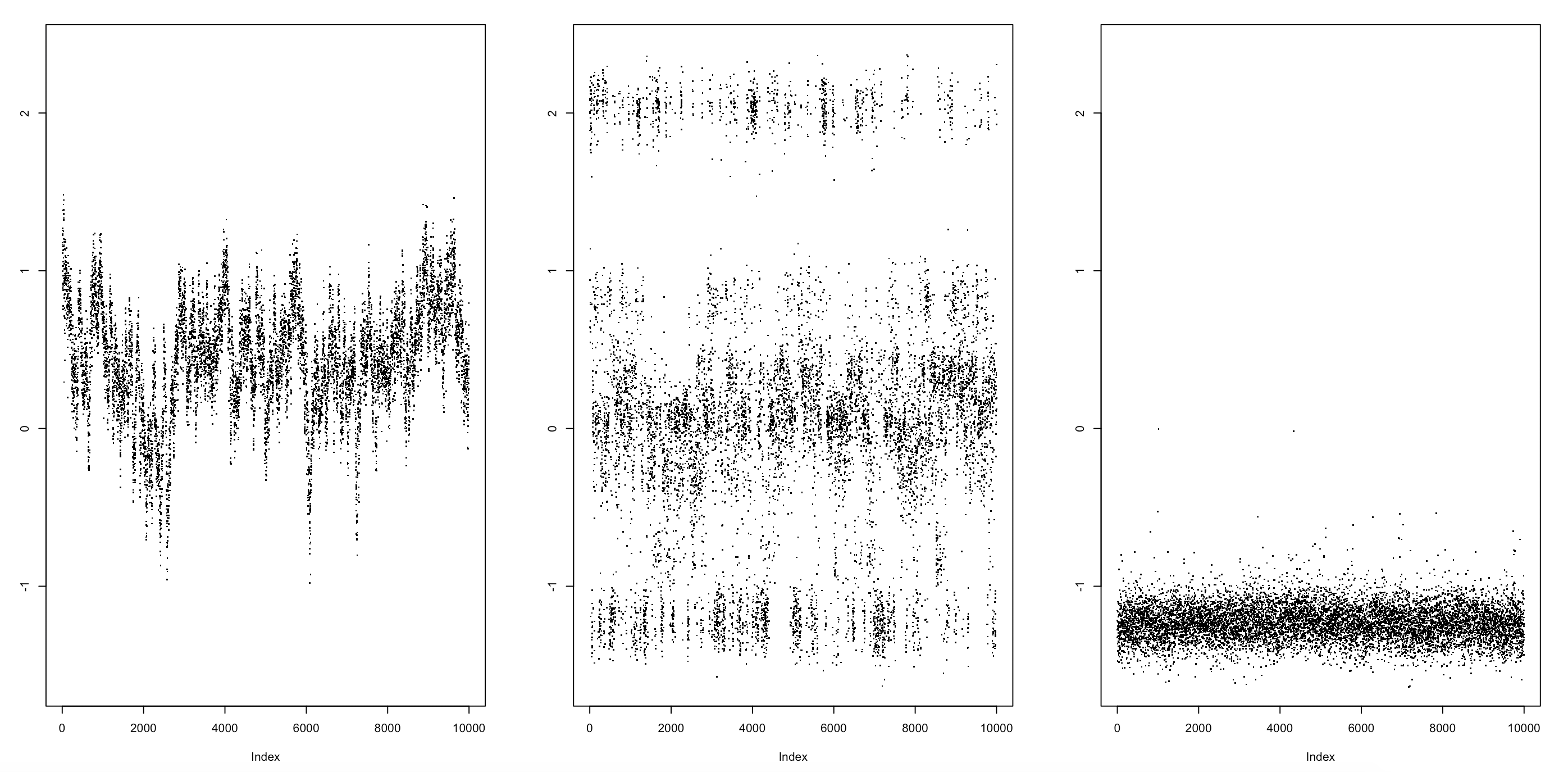
Figure 1: Symptoms of non-identifiability shown in trace plots of one $\Lambda$ entry showing full rotational ambiguity (left), sign and label switching after the application of Varimax (center), and complete alignment after applying MatchAlign (right)

Let $\{\Lambda^{(t)},\ t=1,\ldots,T\}$ be the posterior samples of the factor loading matrix $\Lambda$. Our first goal is to tackle generic rotational invariance across $\Lambda^{(t)}$. In order to achieve that, we apply an orthogonalization procedure to each sample. Orthogonalization of factor loadings highlights the grouping of covariates, often inducing sparsity row-wise in $\Lambda$, which allows the samples to be represented in an interpretable form. Figure 2 shows an example of the application of Varimax to a posterior sample of $\Lambda$. We define as $\tilde{\Lambda}$ the factor loading matrix after applying Varimax. In our approach we focus on orthogonal rotations, and apply Varimax (Kaiser, 1958) to each $\Lambda^{(t)}$. Oblique rotations (Thurstone, 1931) can also provide accurate representations of correlated factors, or more generally linear association in the columns of the unidentifiable matrix. However, the obliquely rotated matrices would not necessarily be comparable across samples.

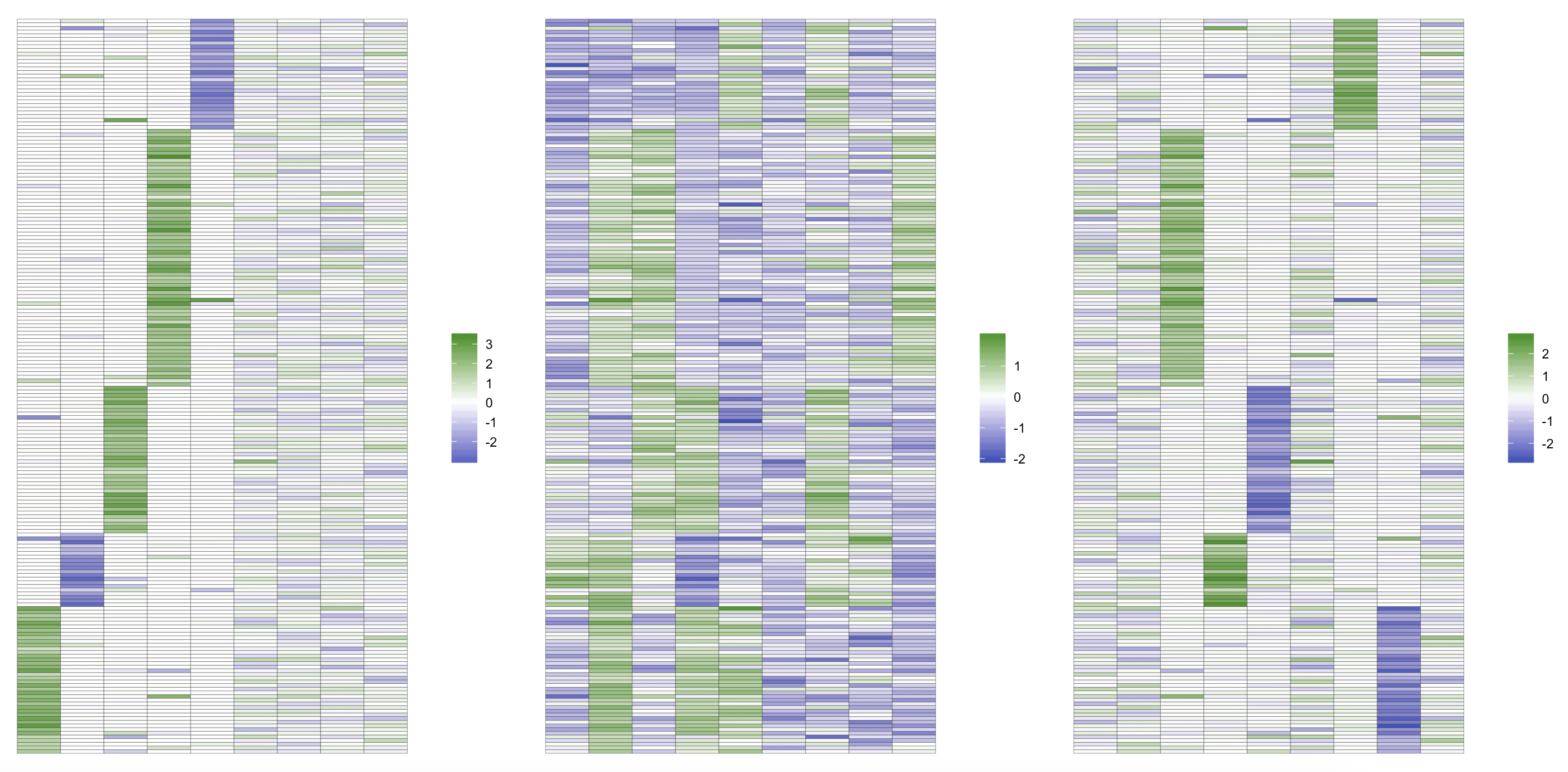
Figure 2: (Left) true factor loadings matrix $\Lambda$ used in simulation, (Center) a posterior sample of $\Lambda$ and (Right) the same sample of $\Lambda$ after applying orthogonalization.

After the orthogonalization step, the samples of $\Lambda$ still exhibit symptoms of non identifiability due to sign and permutation ambiguity in the columns (Conti et al., 2014). Following Papastamoulis and Ntzoufras (2020), we define $Q$ as a $k\times k$ permutation matrix. Each row and column of $Q$ has a single non-zero element, which is equal to $1$. We also define $S=\text{diag}(s_{1},\ldots,s_{k})$, with $s_{j}\in\{-1,1\}$, and $P=SQ$, a signed permutation matrix. Our goal is to find the signed permutation matrices in order to align the samples, and to do that we minimize the following loss function:

$$\text{minimize}_{Q^{(t)},S^{(t)};\ t=1,\ldots,T}\sum_{t=1}^{T}||\tilde{\Lambda}^{(t)}Q^{(t)}S^{(t)}-\Lambda^{P}||_{F}$$ (3)

where $||\cdot||_{F}$ is the Frobenious norm, $\Lambda^{P}=[c_{1}^{P}\cdots\ c_{k}^{P}]$ is an exemplar factor loading matrix, which we call the pivot, and $c_{j}^{(t)}$ is the $j^{th}$ column of $\tilde{\Lambda}^{(t)}$. We use the pivot to align the posterior samples, as in Marin et al. (2005). The pivot matrix is used in the algorithm as a proxy of a ‘true’ $\Lambda$, and we will provide the details of its choice later in this section. The loss function penalizes differences between the pivot and the posterior samples, and to minimize it we must find the signed rearrangement of $c_{1}^{(t)},\ldots,c_{k}^{(t)}$ that best matches the pivot’s columns.

One possibility to minimize (3) is to compute the loss for all possible signed permutations, which is computationally infeasible. Instead, we implement a greedy procedure and minimize the loss iteratively, i.e. column by column, as in Marin et al. (2005). We compute the $L_{2}$ normed differences between the columns of $\tilde{\Lambda}^{(t)}$ and the ones of $\Lambda^{P}$ and $-\Lambda^{P}$. We use the $L_{2}$ norm to match the objective of the Varimax algorithm. Other rotation schemes such as quartimax (Neuhaus and Wrigley, 1954) may work better with the other norms. Our empirical simulations show that MatchAlign is not sensitive to the choice of norm. The computations are implemented in a greedy fashion: we compute the normed differences between the column of $\tilde{\Lambda}^{(t)}$ with largest norm and $c_{1}^{P},-c_{1}^{P},\ldots,c_{k}^{P},\ -c_{k}^{P}$. After matching with $c_{j}^{P}$ or $-c_{j}^{P}$, for some $j=1,\ldots,k$ that minimizes the $L_{2}$ norm, we match the next column of $\tilde{\Lambda}^{(t)}$ with $c_{1}^{P},\ldots,c_{j-1}^{P},-c_{j-1}^{P},c_{j+1}^{P},\ldots,-c_{k}^{P}$ and proceed iteratively. In this way, we only need to compute $k(2k+1)$ normed differences for each posterior sample, and the complexity of the matching step is $\mathcal{O}\big{(}Tpk(2k+1)\big{)}$. Whenever using a prior for $\Lambda$ that introduces increasing shrinkage as the column order increases, as in Bhattacharya and Dunson (2011) or Legramanti et al. (2020), we can naturally start matching the columns from $c_{1}^{(t)}$ and proceed in column order.

Due to sampling noise one $c_{j}^{(t)}$ may be minimally distant from more than one $c_{h}^{P}$. Because of that, we need to avoid matching multiple $c_{j}^{(t)}$s to one $c_{h}^{P}$, which we refer to as duplication. Alignment that involves duplicating some columns over others destroys information and prevents the accurate reconstruction of identifiable parameters such as the covariance after post-processing. Allowing duplication of columns would also introduce numerical instability when performing operations for posterior samples with duplicate columns, as well as biasing ergodic summaries of the parameters.

Several methods for factor models take an “over-fitted” approach (Bhattacharya and Dunson, 2011), (Rousseau and Mengersen, 2011), and choose $k$ to correspond to an upper bound on the number of factors. In this scenario, we might have multiple columns centered near $0_{p}$. For this reason, our algorithm may not detect when these orthogonalized columns switch labels or signs between samples. However, this does not significantly bias the ergodic summaries of the factor loadings. In fact, columns might be mislabelled only if their normed difference is small. This is an important consideration because the matching method does not globally minimize differences between the reference and sample matrices. Instead, it operates on each column iteratively.

In our algorithm, every column of $\Lambda^{(t)}$ is matched to either $c_{j}^{P}$ or $-c_{j}^{P}$, for some $j=1,\ldots,k$. In order to correctly and efficiently match columns, we must choose a pivot that is central in the distribution of a column statistic. As a proxy of unique information contained in each column, we consider the condition number:

$$\kappa^{(t)}=\kappa(\Lambda^{(t)})=\frac{\sigma_{max}(\Lambda^{(t)})}{\sigma_{min}(\Lambda^{(t)})}$$

where $\sigma_{max}(\Lambda^{(t)})$ and $\sigma_{min}(\Lambda^{(t)})$ are the largest and smallest singular values of $\Lambda^{(t)}$, respectively. We choose as a pivot the matrix with the median condition number. Note that this number may approach infinity with an overspecified number of columns. In this case, we can use the largest singular value in place of the condition number. We find in practice that these two choices provide similar performance of MatchAlign. One possibility to run the algorithm without selecting a pivot is by employing the solution of Papastamoulis and Ntzoufras (2020) based on the work of Stephens (2000) in the context of mixture models. However, this solution would involve a significant increase in computational cost. Finally, notice that the identifiable parameters, such as $\Lambda\Lambda^{T}$, are not affected by applying MatchAlign, since we process the samples of $\Lambda$ by post-multiplying with a semi-orthogonal matrix.

4 Simulations

In this section we compare the performance of MatchAlign with three strategies of the Varimax-RSP algorithm of Papastamoulis and Ntzoufras (2020): the Exact scheme (rsp exact), the fastest implementation with full simulated Annealing (RSP full-SA), and a hybrid implementation of the two strategies (RSP partial-SA). We generate $500$ data points according to (1) in two ways: 1) Independent, by sampling each element of $\Lambda$ independently from a standard normal distribution and 2) Sparse, by dividing the covariates in three groups such that each of the groups mainly loads on a single latent factor. We generate the diagonal elements of $\Sigma$ from independent inverse-gamma distributions with parameters $(1/2,1/2)$.

We fit a Gaussian factor model with a Dirichlet-Laplace prior (Bhattacharya et al., 2015) for each row of $\Lambda$ and an inverse-gamma prior with parameters $(1/2,1/2)$ on the diagonal elements of the matrix $\Sigma$. We do not enforce any identifiability constraints on the matrix $\Lambda$. We use the function linearDL contained in infinitefactor R package to draw MCMC samples. We run the MCMC algorithm for $11000$ iterations and a burn-in of $1000$, keeping $10000$ in total. Notice that the run-times of the algorithms are independent of the number of observations since the input of the algorithms is $\{\Lambda^{(t)}:t=1,...,T\}$, which does not depend on $n$. We run the simulations for different values of $p$ and $k$, and for each set of parameters we average the run-times of the four algorithms over $25$ simulations. The alignment times were comparable over the Independent and Sparse settings so for this simulation we also average the results over these two scenarios.

The results are shown in Figure 3 with the run-times on the $\text{log}_{10}$ scale. Notice how the MatchAlign algorithm is often at least an order of magnitude faster (approximately 10 times faster) than RSP full-SA when $k=5,10$, and two orders of magnitude faster (approximately 100 times faster) when $k=25,50$. In Figure 4 we show the run-times in log₁₀ scale between MatchAlign and RSP full-SA and RSP partial-SA across multiple specifications of the number of iterations taken by the MCMC sampler. Again, the difference between MatchAlign and the two implementations of the RSP algorithm is at least an order of magnitude.

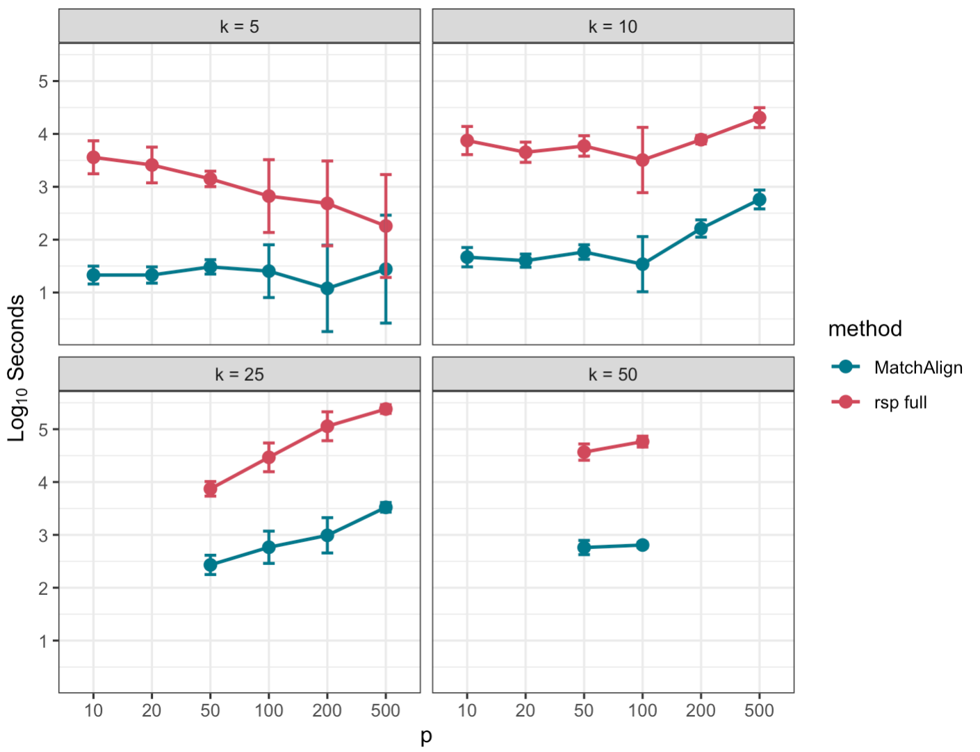
Figure 3: Comparison of running times in log₁₀ scale between MatchAlign and RSP with full-SA.

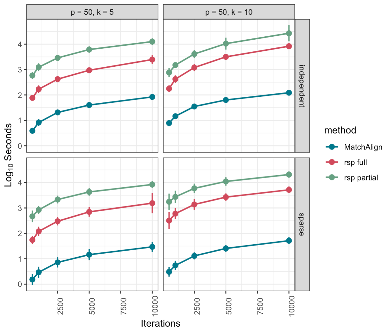
Figure 4: Comparison of running times in log₁₀ scale between MatchAlign and RSP with full-SA across multiple specifications of the number of MCMC iterations.

In order to evaluate the performance of the alignment procedures, one possibility is to use the normed difference between the posterior mean of the covariance and the estimated covariance using the posterior mean of the aligned $\Lambda$:

$$||\overline{\Lambda\Lambda^{T}}-\bar{\Lambda}_{*}\bar{\Lambda}_{*}^{T}||_{F}$$ (4)

where $\overline{\Lambda\Lambda^{T}}=\frac{1}{T}\sum_{t=1}^{T}\Lambda^{(t)}(\Lambda^{(t)})^{T}$ and $\bar{\Lambda}_{*}=\frac{1}{T}\sum_{t=1}^{T}\Lambda^{(t)}_{*}$ is the posterior mean of the aligned $\Lambda$. This follows from the intuition that inference under the rotated $\Lambda$ for the covariance matrix should not largely deviate from the posterior mean of the covariance, if the columns have been aligned correctly. The metric (4) does not necessitate knowing the underlying true parameters, so it can be computed on real data as well.

We compute metric (4) on the simulated data for $k=5,10$ and $p=50,100$. We show the results in Table 1 and 2. As expected, RSP Exact attains the best performance. However, MatchAlign’s results are better than the fastest implementation of RSP and generally comparable to those of RSP Exact, which can only be run for $k\leq 10$.

We also compare the performance of the algorithms by estimating the effective sample size (ESS) after performing alignment. We average ESS over each element in $\Lambda$ and divide by the total number of samples. Generally, if the samples are not aligned correctly then the MCMC will experience poor mixing. We use ESS to compare the different methods but the ratio of ESS over the number of samples should not be close to one as, even with perfect alignment, MCMC algorithms will not produce uncorrelated samples from the posterior. We show the results in Table 3 and 4. Notice how MatchAlign performs similarly to the other algorithms while being at least one order of magnitude faster.

Table 1: Comparison of MatchAlign, RSP full-SA, RSP partial-SA and RSP Exact when $p=50$ according to metric (4). The metric values are presented as ratios compared to the best performing algorithm.

		MatchAlign	RSP exact	RSP full	RSP partial
$\Lambda$ sparse	k=5	$3.548$	$1$	$3.563$	$1.000$
	k=10	$1.331$	$1$	$3.941$	$1.134$
$\Lambda$ independent	k=5	$1$	$1.033$	$1.613$	$1.033$
	k=10	$1.176$	$1$	$1.488$	$1.009$

Table 2: Comparison of MatchAlign, RSP full-SA, RSP partial-SA and RSP Exact when $p=100$ according to metric (4). The metric values are presented as ratios compared to the best performing algorithm.

		MatchAlign	RSP exact	RSP full	RSP partial
$\Lambda$ sparse	k=5	$2.835$	$1$	$1.191$	$1.000$
	k=10	$1.303$	$1$	$2.501$	$1.053$
$\Lambda$ independent	k=5	$1.033$	$1$	$2.262$	$1.001$
	k=10	$1.260$	$1$	$1.321$	$1.010$

Table 3: Comparison of the MatchAlign, RSP full-SA, RSP partial-SA and RSP Exact when $p=50$ using ESS divided by the total number of samples.

		MatchAlign	RSP exact	RSP full	RSP partial
$\Lambda$ sparse	k = 5	$0.686$	$0.630$	$0.646$	$0.635$
	k = 10	$0.797$	$0.738$	$0.826$	$0.783$
$\Lambda$ independent	k = 5	$0.465$	$0.522$	$0.496$	$0.525$
	k = 10	$0.380$	$0.417$	$0.523$	$0.423$

Table 4: Comparison of MatchAlign, RSP full-SA, RSP partial-SA and RSP Exact when $p=100$ using ESS divided by the total number of samples.

		MatchAlign	rsp exact	rsp full	rsp partial
$\Lambda$ sparse	k = 5	$0.728$	$0.641$	$0.644$	$0.641$
	k = 10	$0.819$	$0.782$	$0.854$	$0.789$
$\Lambda$ independent	k = 5	$0.312$	$0.305$	$0.325$	$0.307$
	k = 10	$0.257$	$0.264$	$0.357$	$0.276$

5 Application

We are particularly motivated by studies of environmental health collecting data on mixtures of chemical exposures. These exposures can be moderately high-dimensional with high correlations within blocks of variables; for example, this can arise when an individual is exposed to a product having a mixture of chemicals and when chemical measurements consist of metabolites or breakdown products of a parent compound. In this application, we use data from the National Health and Nutrition Examination Survey (NHANES) collected in 2015 and 2016. We select a subset of $107$ chemical exposures for which at least $30\%$ of measurements have been recorded (i.e., are not missing). We also select a subsample of $4468$ individuals for which at least $30\%$ of the $107$ chemicals have been recorded. After this preprocessing step, we are left with a matrix $X$ of dimension $4468\times 107$ with $36\%$ missing data.

We implement an initial Bayesian analysis of model (1) with the prior of Bhattacharya and Dunson (2011) for $\Lambda$ and an inverse-gamma prior with parameters $(1/2,1/2)$ on the diagonal elements of the matrix $\Sigma$, as in the simulation experiments. We notice from the eigen-decomposition of the correlation matrix that the first $25$ eigenvectors explain more than $80\%$ of the total variability; hence, we set the number of factors equal to $25$. We run the MCMC procedure for $11000$ iterations with a burn-in of $10000$ and apply the MatchAlign and RSP-full algorithms to the posterior samples of $\Lambda$.

Figure 5 shows the aligned posterior mean for the factor loadings matrix for the $107$ chemical exposures. We re-ordered the rows of $\Lambda$ to highlight the chemical groupings. The time to align the samples using MatchAlign was around $16$ seconds on a single thread of a 4.5GHz processor. Figure 6 shows the traceplots of $\Lambda_{11},\ldots,\Lambda_{16}$ before and after rotation. RSP-Full fails to properly align some samples resulting in biased estimates. The value of the metric (4) was approximately $20$ times higher for RSP-Full compared to MatchAlign.

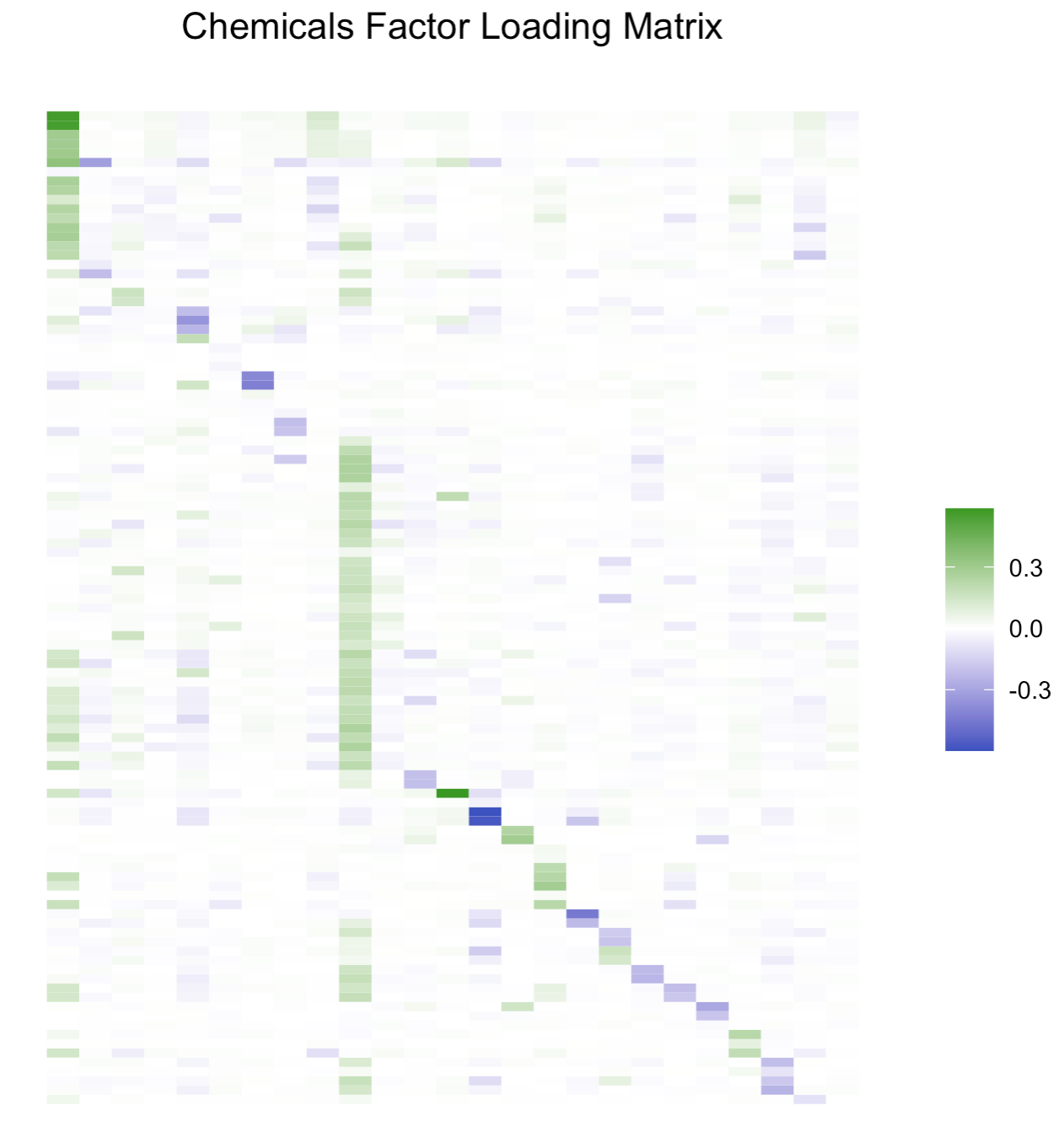
Figure 5: Matrix of factor loadings for NHANES 2015-2016 dataset after postprocessing with MatchAlign algorithm.

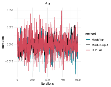
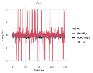
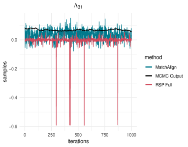
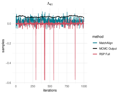
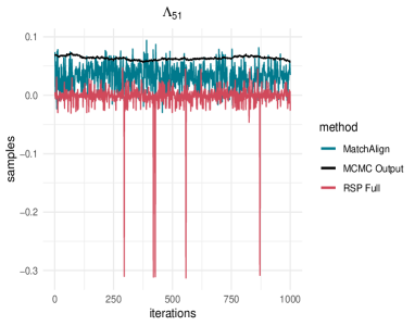
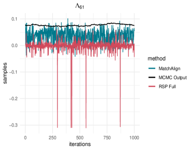
Figure 6: Traceplots of the factor loadings $\Lambda_{11},\ldots,\Lambda_{16}$ before and after rotation with MatchAlign and RSP-Full.

6 Discussion

We proposed a computationally efficient post-processing algorithm that solves label and sign switching in matrix valued parameters that are subject to rotational ambiguity. Solving rotational ambiguity for high-dimensional parameters in Bayesian models can be challenging because of the of high computational cost. Our MatchAlign algorithm reduces the solution space by iteratively comparing columns, saving massive computational time in comparison to permutation searches, as in Papastamoulis and Ntzoufras (2020). In Section 4 we compared the computational performance of MatchAlign with respect to the algorithm of Papastamoulis and Ntzoufras (2020) and show that MatchAlign is at least one order of magnitude faster, without compromising the performance of alignment.

Crucially, this algorithm does not alter the estimation of identifiable parameters, such as $\Lambda\Lambda^{T}$, and allows one to perform inference on the factor loadings matrix. The code is available in the infinitefactor R package on the CRAN repository and can be easily applied in broad settings.

References

- Anderson et al. (1956) Anderson, T. W., H. Rubin, et al. (1956). Statistical inference in factor analysis. In Proceedings of the third Berkeley symposium on mathematical statistics and probability, Volume 5, pp. 111–150.
- Aßmann et al. (2016) Aßmann, C., J. Boysen-Hogrefe, and M. Pape (2016). Bayesian analysis of static and dynamic factor models: An ex-post approach towards the rotation problem. Journal of Econometrics 192(1), 190–206.
- Bhattacharya and Dunson (2011) Bhattacharya, A. and D. B. Dunson (2011). Sparse Bayesian infinite factor models. Biometrika 98, 291–306.
- Bhattacharya et al. (2015) Bhattacharya, A., D. Pati, N. S. Pillai, and D. B. Dunson (2015). Dirichlet–laplace priors for optimal shrinkage. Journal of the American Statistical Association 110(512), 1479–1490.
- Carvalho et al. (2008) Carvalho, C. M., J. Chang, J. E. Lucas, J. R. Nevins, Q. Wang, and M. West (2008). High-dimensional sparse factor modeling: applications in gene expression genomics. Journal of the American Statistical Association 103(484), 1438–1456.
- Chen et al. (2020) Chen, Y., X. Li, and S. Zhang (2020). Structured latent factor analysis for large-scale data: Identifiability, estimability, and their implications. Journal of the American Statistical Association 115(532), 1756–1770.
- Conti et al. (2014) Conti, G., S. Frühwirth-Schnatter, J. J. Heckman, and R. Piatek (2014). Bayesian exploratory factor analysis. Journal of econometrics 183(1), 31–57.
- Erosheva and Curtis (2011) Erosheva, E. A. and S. M. Curtis (2011). Dealing with rotational invariance in bayesian confirmatory factor analysis. Department of Statistics, University of Washington, Seattle, Washington, USA.
- Frühwirth-Schnatter and Lopes (2018) Frühwirth-Schnatter, S. and H. F. Lopes (2018). Sparse bayesian factor analysis when the number of factors is unknown. arXiv preprint arXiv:1804.04231.
- Geweke and Zhou (1996) Geweke, J. and G. Zhou (1996). Measuring the pricing error of the arbitrage pricing theory. The Review of Financial Studies 9(2), 557–587.
- Ghosh and Dunson (2009) Ghosh, J. and D. B. Dunson (2009). Default prior distributions and efficient posterior computation in bayesian factor analysis. Journal of Computational and Graphical Statistics 18(2), 306–320. PMID: 23997568.
- Kaiser (1958) Kaiser, H. F. (1958, Sep). The varimax criterion for analytic rotation in factor analysis. Psychometrika 23(3), 187–200.
- Kaufmann and Schumacher (2017) Kaufmann, S. and C. Schumacher (2017). Identifying relevant and irrelevant variables in sparse factor models. Journal of Applied Econometrics 32(6), 1123–1144.
- Kaufmann and Schumacher (2019) Kaufmann, S. and C. Schumacher (2019). Bayesian estimation of sparse dynamic factor models with order-independent and ex-post mode identification. Journal of Econometrics 210(1), 116–134.
- Lawley and Maxwell (1962) Lawley, D. N. and A. E. Maxwell (1962). Factor analysis as a statistical method. Journal of the Royal Statistical Society: Series D (The Statistician) 12(3), 209–229.
- Legramanti et al. (2020) Legramanti, S., D. Durante, and D. B. Dunson (2020). Bayesian cumulative shrinkage for infinite factorizations. Biometrika 107(3), 745–752.
- Lorenzo-Seva (1999) Lorenzo-Seva, U. (1999). Promin: A method for oblique factor rotation. Multivariate Behavioral Research 34(3), 347–365.
- Lucas et al. (2006) Lucas, J., C. Carvalho, Q. Wang, A. Bild, J. R. Nevins, and M. West (2006). Sparse statistical modelling in gene expression genomics. Bayesian Inference for Gene Expression and Proteomics 1(1).
- Marin et al. (2005) Marin, J.-M., K. L. Mengersen, and C. Robert (2005, 12). Bayesian modelling and inference on mixtures of distributions. Handbook of Statistics 25.
- McAlinn et al. (2018) McAlinn, K., V. Rockova, and E. Saha (2018). Dynamic sparse factor analysis. arXiv preprint arXiv:1812.04187.
- Millsap (2001) Millsap, R. E. (2001). When trivial constraints are not trivial: The choice of uniqueness constraints in confirmatory factor analysis. Structural Equation Modeling 8(1), 1–17.
- Neuhaus and Wrigley (1954) Neuhaus, J. O. and C. Wrigley (1954). The quartimax method: an analytic approach to orthogonal simple structure. British Journal of Statistical Psychology 7(2), 81–91.
- Papastamoulis and Ntzoufras (2020) Papastamoulis, P. and I. Ntzoufras (2020). On the identifiability of Bayesian factor analytic models. arXiv preprint arXiv:2004.05105.
- Rousseau and Mengersen (2011) Rousseau, J. and K. Mengersen (2011). Asymptotic behaviour of the posterior distribution in overfitted mixture models. Journal of the Royal Statistical Society: Series B (Statistical Methodology) 73(5), 689–710.
- Stephens (2000) Stephens, M. (2000). Dealing with label switching in mixture models. Journal of the Royal Statistical Society: Series B (Statistical Methodology) 62(4), 795–809.
- Thurstone (1931) Thurstone, L. L. (1931). Multiple factor analysis. Psychological review 38(5), 406.