Generalizing Gaze Estimation with Outlier-guided Collaborative Adaptation

Abstract

Deep neural networks have significantly improved appearance-based gaze estimation accuracy. However, it still suffers from unsatisfactory performance when generalizing the trained model to new domains, e.g., unseen environments or persons. In this paper, we propose a plug-and-play gaze adaptation framework (PnP-GA), which is an ensemble of networks that learn collaboratively with the guidance of outliers. Since our proposed framework does not require ground-truth labels in the target domain, the existing gaze estimation networks can be directly plugged into PnP-GA  and generalize the algorithms to new domains. We test PnP-GA  on four gaze domain adaptation tasks, ETH-to-MPII, ETH-to-EyeDiap, Gaze360-to-MPII, and Gaze360-to-EyeDiap. The experimental results demonstrate that the PnP-GA  framework achieves considerable performance improvements of 36.9%, 31.6%, 19.4%, and 11.8% over the baseline system. The proposed framework also outperforms the state-of-the-art domain adaptation approaches on gaze domain adaptation tasks. Code has been released at https://github.com/DreamtaleCore/PnP-GA.

1 Introduction

Eye gaze is an important indicator of human attention. It has been exploited in various applications, such as human-robot interaction [1, 28, 30], virtual/augmented reality games [2, 20, 32], intelligent cockpit systems [12], medical analysis [4], etc. With the development of deep learning techniques, appearance-based gaze estimation attracts much attention recently. To improve gaze estimation accuracy, many large-scale gaze estimation datasets have been proposed [10, 19, 35, 37]. Due to the differences of subjects, background environments, and illuminations between these datasets, the performance of gaze estimation models that are trained on a single dataset usually dramatically degrades when testing on a new dataset.

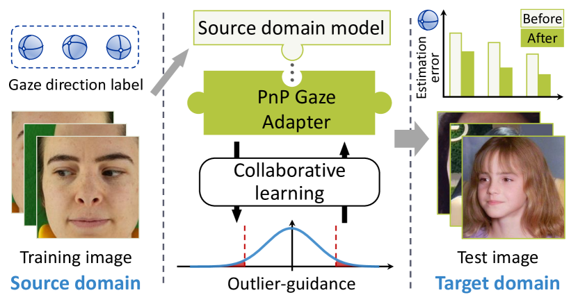
Figure 1: Overview of the proposed Plug-and-Play (PnP) adaption framework for generalizing gaze estimation to a new domain.

To tackle such a gap in gaze estimation, several works have been proposed by utilizing adversarial training (ADV) [26, 31], few-shot learning (FSL) [25, 33], or embedding with prediction consistency [14]. However, these works mainly focus on the inter-person gap (i.e., personal calibration) from the same dataset, where the environmental conditions are often very similar. When generalizing the gaze estimation models to new datasets, the differences between the image capture devices and the environments cannot be neglected, as illustrated in Fig. 1. Consequently, a gaze estimation model trained in the source domain cannot achieve satisfactory performance by directly applying to the target domain. In this paper, we focus on domain adaptation between different datasets, which is more common in practical applications.

Unlike most of the existing works in gaze domain adaptation following supervised learning paradigm, this work aims to generalize the gaze estimation in an unsupervised manner. This is because we usually do not have access to the ground-truth labels in a new domain. The task can be viewed as an unsupervised domain adaptation (UDA) problem. Table 1 shows the differences between the existing gaze domain adaptation approaches and UDA. While the ADV and FSL approaches are model-specific, the UDA and fine-tuning approaches are model-agnostic. It means that these methods are capable of adapting arbitrary network architectures. However, the fine-tuning approach requires a number of target labels. The UDA approach is more challenging than conventional approaches since the lack of annotated data in a new domain prohibits fine-tuning of the pre-trained models. Many UDA methods for other computer vision tasks have explored to take additional priors, e.g., shape priors for hand segmentation [3], pseudo labels for person re-identification [11], random sampler [21] for head pose estimation, etc. However, the aforementioned priors are not available on gaze estimation tasks, since gaze directions have no specific shapes or labels.

Table 1: Differences among the domain adaptation approaches.

Methods	# Target images	# Target labels	Model
Fine-tuning	$\blacksquare\blacksquare\blacksquare\blacksquare\blacksquare$	$\blacksquare\blacksquare\blacksquare\blacksquare\blacksquare$	Agnostic
FSL [25, 33]	$\blacksquare$	$\blacksquare$	Specific
ADV [26, 31]	$\blacksquare\blacksquare$	Not require	Specific
UDA (Ours)	$\blacksquare$	Not require	Agnostic

In this paper, we propose an outlier-guided plug-and-play collaborative learning framework for generalizing gaze estimation with unsupervised domain adaptation. Optimizing the error-prone outliers has been proved to be helpful for model generalization [18, 34]. We follow the similar idea and take the outliers of pre-trained models’ outputs in the target domain as noisy labels. We employ two groups of networks that collaboratively teach each other. While these two groups share the same architecture, one group is the momentum version of another group. The primary contributions of this paper are summarized as follow:

• We propose a plug-and-play gaze adaptation framework (PnP-GA) for generalizing gaze estimation in new domains. Existing gaze estimation networks can be easily plugged into our framework without modification of their architectures.

• We propose an outlier-guided collaborative learning strategy for the unsupervised domain adaptation. It only requires a few samples from the target domain without any labels. We specifically design an outlier-guided loss to better characterize the outliers and guide the learning.

• The PnP-GA framework shows exceptional performances with plugging of the existing gaze estimation networks. Our system achieves performance improvements over the baseline system of 36.9%, 31.6%, 19.4% and 11.8% on four gaze adaptation tasks: ETH-to-MPII, ETH-to-EyeDiap, Gaze360-to-MPII and Gaze360-to-EyeDiap.

2 Related Works

2.1 Gaze estimation

Appearance-based gaze estimation methods have gradually become a research hotspot. Recent studies have significantly improved the gaze estimation accuracy on public datasets by using coarse-to-fine strategy[7], domain adaptation[14, 26], and adversarial learning approach[31].

However, Most studies investigate the person-specific adaptation of gaze estimators within the same dataset[24, 25, 33], the model generalization across the dataset is often ignored in previous studies. Such task is rather challenging due to the huge differences of the distribution between different datasets. Considering the diversity of the real-world environment, even if the model performs well within the dataset, it is difficult to apply to practical applications. More recently, ETH-XGaze[35], Gaze360[19], etc. large-scale gaze datasets with a wider distribution have been proposed, which have greatly promoted the development of gaze estimation to practical applications. Recent work [35] has begun to consider the cross dataset generalization capabilities of gaze estimation methods. Here, we propose an unsupervised approach to improve the cross-dataset and cross-domain performance of gaze estimation methods.

2.2 Unsupervised domain adaptation

Unsupervised domain adaptation has been extensively explored in deep learning field. Previous unsupervised domain adaptation approaches can be categorized into two techniques: adversarial learning and self-training. Adversarial learning based approaches are motivated by generative adversarial networks(GAN)[13]. A large number of such methods have been developed, such as ADDA[29], CDAN[23], CyCADA[17], Symnets[38], GVBGD[8], etc. The key idea is to make the domain discriminator and the generator play a min-max game, thereby it explicitly reduces the distance between the source domain and the target domain. Self-training based approaches are motivated by semi-supervised learning[22, 27], which usually trains the model using the reliable predictions of itself, such as Pseudo-label method[22], Mean Teacher method[27], etc. Recent works [3, 5, 9, 40] apply self-training to unsupervised domain adaptation, and achieve significant results. Compared with adversarial learning, although the self-training methods can only perform feature alignment implicitly, the adaptation performance is usually better.

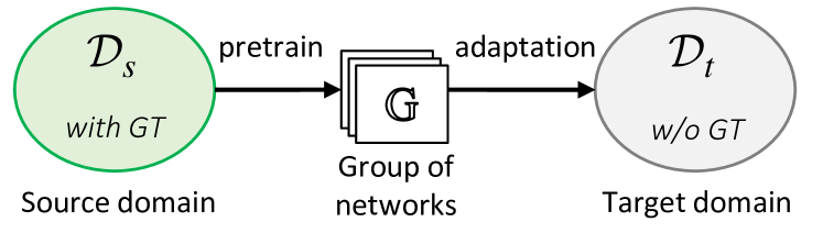
Figure 2: Illustration of unsupervised domain adaptation for gaze estimation.

However, the majority of the previous domain adaptation works focus on classification tasks rather than regression tasks. For gaze domain adaptation, unsupervised domain adaptation is even difficult due to the continuity nature of gaze directions. Thus, there still remains much space to be explored.

3 Task Definition

Fig.2 illustrates the unsupervised domain adaptation for gaze estimation. We denote the source domain data as $\mathcal{D}_{s}=\{(\mathbf{x}^{s}_{i},\mathbf{y}^{s}_{i})|_{i=1}^{N_{s}}\}$, where $\mathbf{x}^{s}_{i}$ and $\mathbf{y}^{s}_{i}$ denote the i-th training image and the corresponding gaze direction, $N_{s}$ is the number of images, $\mathbf{y}^{s}_{i}$ contains the pitch and yaw angle of the gaze direction. The target domain data is denoted as $\mathcal{D}_{t}=\{(\mathbf{x}^{t}_{i})|_{i=1}^{N_{t}}\}$, where $N_{t}$ is the number of images, $\mathbf{x}^{t}_{i}$ is the i-th image. It contains no ground-truth gaze direction.

Suppose we have a group of baseline gaze estimation models $\mathbb{G}=\{G(\centerdot|\theta_{k})|_{k=1}^{H}\}$ with parameters $\theta_{k}$ learned using training data from the source domain $\mathcal{D}_{s}$, where $H$ is the number of models. The pre-trained baseline models may not generalize to a target domain since the test samples from $\mathcal{D}_{t}$ and $\mathcal{D}_{s}$ usually have different distributions. Our task is to adapt the pre-trained models to the new domain $\mathcal{D}_{t}$ without requiring any ground-truth labels.

Datasets. Four different datasets are employed as four different domains: ETH-XGaze ($\mathcal{D}_{E}$), Gaze360 ($\mathcal{D}_{G}$), MPIIGaze ($\mathcal{D}_{M}$) and EyeDiap ($\mathcal{D}_{D}$). The details of the datasets are as follows:

ETH-XGaze dataset ($\mathcal{D}_{E}$) [35] is collected under adjustable illumination conditions and a custom hardware setup.

Gaze360 dataset ($\mathcal{D}_{G}$) [19] consists of 238 subjects in indoor and outdoor environments.

MPIIGaze dataset ($\mathcal{D}_{M}$) [37] is collected from 15 subjects in real-world environments. Therefore it has various illumination conditions.

EyeDiap dataset ($\mathcal{D}_{D}$) [10] consists of a number of video clips from 16 subjects, which are collected under screen targets or 3D floating balls.

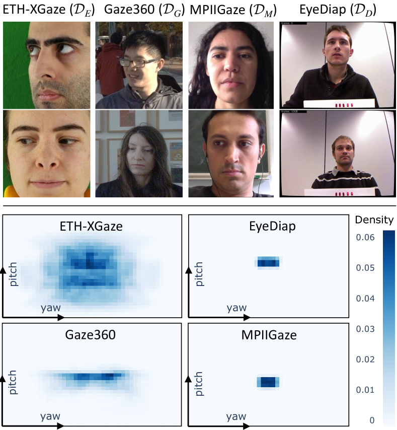
Figure 3: Illustration of four gaze datasets. Top: Image samples. Large variation on illumination and background could be observed across datasets. Bottom: Gaze direction distributions. The x,y axes show the yaw and pitch angle.

Image samples and gaze direction distributions of these datasets are shown in Fig. 3. By assuming the source domain has wider distributions than target domain, we find that the gaze distributions of ETH-XGaze and Gaze360 are significantly larger than EyeDiap and MPIIGaze dataset, therefore we utilize ETH-XGaze and Gaze360 as source domains to pre-train models, and use MPIIGaze and EyeDiap as target domains for adaptation. It is noted that 1) we use gaze direction labels in ETH-XGaze and Gaze360 dataset for training the gaze estimation network and 2) labels in other datasets are only used for performance evaluation.

4 Proposed Approach

We propose a novel Plug-and-Play Gaze Adaptation (PnP-GA) framework with outlier-guidance and collaborative learning. The architecture overview is illustrated in Fig. 4. Our key idea is to guide the learning by the prediction outliers. We introduce a novel outlier-guided loss to better utilize the outliers for generalizing gaze estimation models. The proposed framework contains two branches, group $\mathbb{G}$ and group $\overline{\mathbb{G}}$, which collaboratively learn from each other. The PnP-GA  framework is model agnostic and existing gaze estimation networks can be directly plugged into it without any modifications.

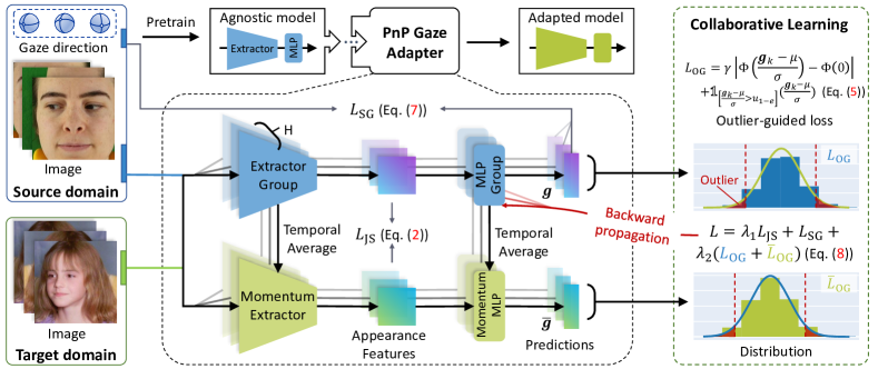
Figure 4: Overview of the proposed PnP-GA framework. At first, a group of pre-trained models (with members’ number $=H$) are plugged into our PnP-GA. The architecture of PnP-GA  is illustrated in the dark dashed box. Then a few samples from the source domain and the target domain are used for adaptation. In the next, our PnP-GA  collaboratively learns from both domains (Sec. 4.1). During adaptation, an outlier-guided loss is proposed to better characterize the property of outliers (Sec 4.2). After adaptation, the first member of the model group is used as an adapted model, which achieves a better performance in the target domain.

4.1 Model agnostic collaborative learning

The PnP-GA framework employs two groups of networks that learn collaboratively. The group $\mathbb{G}$ generates gaze direction predictions with different pre-trained weights from the source domain. A network $G$ from $\mathbb{G}$ contains a feature extractor, which follows a multi-layer perceptron (MLP). While another group $\overline{\mathbb{G}}$ is the momentum version of group $\mathbb{G}$. A network $\overline{G}$ from the momentum group $\overline{\mathbb{G}}$ takes the temporal average of the feature extractor and MLP from the corresponding network in group $\mathbb{G}$. The PnP-GA framework is model agnostic since we use a generic network architecture, which consists of a feature extraction stage and a feature mapping stage. Such an architecture has been widely used in gaze estimation studies [6, 7, 36]. Thus, different gaze estimation models can be easily plugged into the proposed PnP-GA  framework.

We denote the feature extraction function of the k-th network in group $\mathbb{G}$ as $F(\centerdot|\theta_{k})$, the multi-layer perceptron of the k-th network in group $\mathbb{G}$ as $\Pi(\centerdot|\theta_{k})$. Then, the k-th network $G(\centerdot|\theta_{k})$ in group $\mathbb{G}$ can be expressed as $F(\centerdot|\theta_{k})\circ\Pi(\centerdot|\theta_{k})$. One straightforward way to generalize these networks to a target domain is to directly compute a loss from the outputs of themselves. However, the estimation errors might amplify during generalizing this way. To overcome error amplification, we propose to use the temporal average of these models to generate reliable appearance features and predictions. Specifically, the parameters of the k-th model from the temporal average group at current iteration $T$ are denoted as $E^{(T)}[\theta_{k}]$, which can be updated as:

$$E^{(T)}[\theta_{k}]=\alpha E^{(T-1)}[\theta_{k}]+(1-\alpha)\theta_{k},$$ (1)

where $E^{(T-1)}[\theta_{k}]$ indicates the temporal average parameters of the k-th network in the previous iteration $T-1$, and $\alpha$ represents the ensembling momentum, which is usually set as 0.99 [11, 16]. We utilize the robust appearance feature $\overline{z_{k}}$, which is generated by the k-th momentum network as $\overline{F}(x|E[\theta_{k}])$ to constrain the k-th appearance feature $z_{k}$, where $E[\theta_{k}]$ is the temporal average parameters of $\theta_{k}$. Specifically, we follow the work in [39] and minimize the symmetric Jensen-Shannon (JS) divergence between $\overline{z_{k}}$ and $z_{k}$ as follow:

$$L_{\mathrm{JS}}=\frac{1}{2}(L_{\mathrm{KL}}(z_{k}\parallel\overline{z_{k}})+L_{\mathrm{KL}}(\overline{z_{k}}\parallel z_{k})),$$ (2)

where $L_{\mathrm{KL}}(p\parallel q)$ is the Kullback Leibler (KL) divergence from $q$ to $p$, which is computed as:

$$L_{\mathrm{KL}}(p\parallel q)=\sum_{t}\log\frac{p(t)}{q(t)}.$$ (3)

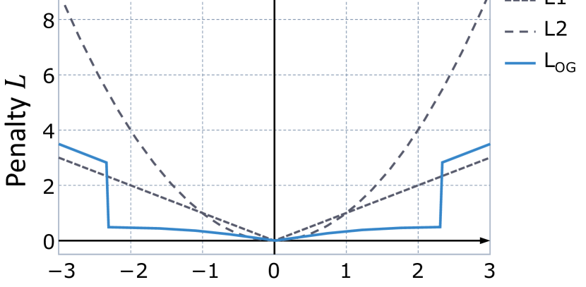
Figure 5: Comparison of the proposed outlier-guided loss $L_{\mathrm{OG}}$, $L1$ loss, and $L2$ loss.

4.2 Outlier-guided loss function

We specially design a loss function to better characterize the property of outliers. Suppose we have $H$ members in group $\mathbb{G}$ and group $\overline{\mathbb{G}}$ respectively, as illustrated in Fig. 4. These networks output predictions $\mathbf{g}_{k}=G(\mathbf{x}|\theta_{k})$, $\mathbf{\overline{g}}_{k}=\overline{G}(\mathbf{x}|E[\theta_{k}])$, where $k=1,...,H$. As mentioned in Sec. 4.1, we make these two groups of networks guide each other to avoid error amplification. Specifically, we calculate a normal distribution by estimating the mean $\mu$ and variance $\sigma^{2}$ of the momentum group’s predictions using the following equations:

$$\mu=\frac{1}{H}\sum_{k=1}^{H}\mathbf{\overline{g}}_{k},~{}~{}\sigma^{2}=\frac{1}{H-1}\sum_{k=1}^{H}(\mathbf{\overline{g}}_{k}-\mu)^{2}.$$ (4)

Here we define the output $\mathbf{g}_{k}$ as a reliable output when $|\frac{\mathbf{g}_{k}-\mu}{\sigma}|\leq u_{1-\epsilon}$, where $u$ is the quantile of the standard normal distribution, and $\epsilon$ indicates the significance level of judging an output as an outlier. Then we estimate outliers from group $\mathbb{G}$’s predictions and punish them with a larger gradient. Toward this end, the outlier-guided loss is formulated as follow:

$$L_{\mathrm{OG}}(\mathbf{g}_{k},\mu,\sigma) =\gamma|\Phi(\frac{\mathbf{g}_{k}-\mu}{\sigma})-\Phi(0)|$$ (5)

$$+\mathbbm{1}_{[|\frac{\mathbf{g}_{k}-\mu}{\sigma}|>u_{1-\epsilon}]}|\frac{\mathbf{g}_{k}-\mu}{\sigma}|,$$

where $\Phi$ represents the cumulative distribution function of the standard normal distribution, i.e.,

$$\begin{split}\Phi(x)=\int_{-\infty}^{x}\frac{1}{\sqrt{2\pi}}e^{-\frac{t^{2}}{2}}\text{dt}.\end{split}$$ (6)

For better understanding, we visualize different loss functions of $L1$, $L2$ and $L_{\mathrm{OG}}$ in Fig.5, in which distance $d=\frac{\mathbf{g}_{k}-\mu}{\sigma}$. In our experiments, we empirically choose $\gamma=0.01$, $\epsilon=0.05$. Please refer to Sec. 5.4.3 for the parameter choosing. Similarly, we compute $\overline{L}_{\mathrm{OG}}$ for group $\overline{\mathbb{G}}$’s predictions.

Source domain constraint. Besides the information obtained from the target domain, we find it also important to fully exploit the gaze information from the source domain. The gaze information of the source domain is learned by minimizing the distance between the model predictions $\mathbf{g}^{s}$ and the ground-truth labels $\mathbf{y}^{s}$, i.e.,

$$L_{\mathrm{SG}}(\mathbf{g^{s}},\mathbf{y}^{s})=|\mathbf{g^{s}}-\mathbf{y}^{s}|,$$ (7)

Total loss. The total loss of the proposed system is a combination of several loss functions, which can be written as follow:

$$L=\lambda_{1}L_{\mathrm{JS}}+L_{\mathrm{SG}}+\lambda_{2}(L_{\mathrm{OG}}+\overline{L}_{\mathrm{OG}}),$$ (8)

where $\lambda_{1}$ and $\lambda_{2}$ are tunable parameters. We emprically set $\lambda_{1}=0.01$ and $\lambda_{2}=0.1$ in our experiment.

4.3 Adaptation procedure

We summarize the adaptation procedure in Algorithm 1. We first obtain a group of pre-trained networks $\mathbb{G}$, which contains the top H networks trained on the source domain. The top H networks are selected based on the prediction accuracy. We use a few images with ground-truth labels ($\mathcal{D}_{s}^{\prime}$) from the source domain $\mathcal{D}_{s}$ and a few images ($\mathcal{D}_{t}^{\prime}$) from the target domain $\mathcal{D}_{t}$ for unsupervised adaptation. During the adaptation process, the networks in group $\mathbb{G}$ are trained by minimizing the loss function in Eq. (8), and the momentum networks in group $\overline{\mathbb{G}}$ is updated with Eq. (1).After adaptation, the first member of the model group is used as an adapted model.

Algorithm 1 Outlier-guided domain adaptation algorithm for gaze estimation.

1:Small $\mathcal{D}_{t}^{\prime}$, small $\mathcal{D}_{s}^{\prime}$ and $\mathbb{G}$ pre-trained on $\mathcal{D}_{s}$

2:$G(\centerdot|\theta)$

3:Initialize: $\overline{\mathbb{G}}^{(1)}\leftarrow\mathbb{G}^{(1)}$ $\triangleright$ $\overline{\mathbb{G}}$ is the momentum $\mathbb{G}$.

4:for $T{\leftarrow}1\;to\;N$ do

5:     ($\mathbf{x}_{s}$, $\mathbf{y}_{s}$),  $\mathbf{x}_{t}$ $\leftarrow$ $\mathcal{D}_{s}^{\prime}$,  $\mathcal{D}_{t}^{\prime}$

6:     $L_{JS}$ $\leftarrow$ $\mathbb{G}(\mathbf{x_{t}}|\theta^{(T)})$,  $\overline{\mathbb{G}}(\mathbf{x_{t}}|E^{(T)}[\theta])$ with Eq. (2).

7:     $L_{\mathrm{OG}}$, $\overline{L}_{\mathrm{OG}}$ $\leftarrow$ $\mathbb{G}(\mathbf{x_{t}}|\theta^{(T)})$, $\overline{\mathbb{G}}(\mathbf{x_{t}}|E^{(T)}[\theta])$ with Eq. (5)

8:     $L_{\mathrm{SG}}$ $\leftarrow$ $\mathbf{y}_{s}$,  $\mathbb{G}(\mathbf{x}_{s}|\theta^{(T)})$ with Eq. (7).

9:     Train $\mathbb{G}(\centerdot|\theta^{(T+1)})$ with Eq. (8).

10:     Update $E^{(T+1)}[\theta]$ in $\overline{\mathbb{G}}$ with Eq. (1)

11:end for

12:$G(\centerdot|\theta)\leftarrow\mathbb{G}(\centerdot|\theta)_{1}$

Training details. We employ PyTorch for implementation. All experiments run on a single NVIDIA 2080TI GPU. We use the Adam optimizer with a learning rate of $10^{-4}$ to train the gaze estimation network in the source domain. For model adaptation, we use the Adam optimizer with a learning rate of $10^{-4}$.

5 Experimental Results

5.1 Data preparation

Due to the differences in different dataset, we first do data preparation. Note that our domain adaptation task is to adapt from the source domain (ETH-XGaze or Gaze360 dataset) to the target domain (MPIIGaze or EyeDiap dataset). For the ETH-XGaze dataset [35] ($\mathcal{D}_{E}$), it provides 80 subjects (i.e., 756,540 images) which are used as the training set. For the Gaze360 dataset [19] ($\mathcal{D}_{G}$), we remove images without subjects’ faces and use the remaining 100,933 images as the training set. Since the MPIIGaze[37] ($\mathcal{D}_{M}$) provides a standard evaluation protocol, which selects 3000 images from each subject to form an evaluation set, therefore we adopt the evaluation set directly. For the EyeDiap dataset [10] ($\mathcal{D}_{D}$), we employ 16,674 images from 14 subjects under screen target sessions as the evaluation set.

We follow the approach in [37] to normalize the data. They predict the gaze direction only based on face images. However, the change of head poses will significantly affect the appearance of face image. Thus, we eliminated the influence of different head poses through rotating the virtual camera and wrapping the images.

Table 2: Domain adaptation results of plugging the existing gaze estimation networks into the proposed PnP-GA framework. Angular gaze error (^∘) is used as evaluation metric.

Input	Method	$\mathcal{D}_{E}\rightarrow\mathcal{D}_{M}$	$\mathcal{D}_{E}\rightarrow\mathcal{D}_{D}$	$\mathcal{D}_{G}\rightarrow\mathcal{D}_{M}$	$\mathcal{D}_{G}\rightarrow\mathcal{D}_{D}$
Face	Baseline [15]	8.767	8.578	7.662	8.977
	Baseline [15] + PnP-GA	5.529 $\blacktriangledown$ 36.9%	5.867 $\blacktriangledown$ 31.6%	6.176 $\blacktriangledown$ 19.4%	7.922 $\blacktriangledown$ 11.8%
	ResNet50 [15, 35]	8.017	8.310	8.328	7.549
	ResNet50 [15, 35] + PnP-GA	6.000 $\blacktriangledown$ 25.2%	6.172 $\blacktriangledown$ 25.7%	5.739 $\blacktriangledown$ 31.1%	7.042 $\blacktriangledown$ 6.7%
	SWCNN [36]	10.939	24.941	10.021	13.473
	SWCNN [36] + PnP-GA	8.139 $\blacktriangledown$ 25.6%	15.794 $\blacktriangledown$ 36.7%	8.740 $\blacktriangledown$ 12.8%	11.376 $\blacktriangledown$ 15.6%
Face + Eye	CA-Net [7]	-	-	21.276	30.890
	CA-Net [7] + PnP-GA	-	-	17.597 $\blacktriangledown$ 17.3%	16.999 $\blacktriangledown$ 44.9%
	Dilated-Net [6]	-	-	16.683	18.996
	Dilated-Net [6] + PnP-GA	-	-	15.461 $\blacktriangledown$ 7.3%	16.835 $\blacktriangledown$ 11.4%

5.2 Plugging the existing gaze estimation networks

We first plug the existing gaze estimation networks into the PnP-GA  framework to improve their domain adaptation performances. We select several popular gaze estimation networks: ResNet18 [15], ResNet50 [15, 35], SWCNN [36], CA-Net[7] and Dilated-Net [6]. The baseline method is ResNet18 [15]. Two different types of networks are utilized to evaluate our method: 1) ResNet18, ResNet50 and SWCNN only require facial images as input, and 2) CA-Net and Dilated-Net require both face and eye images as input. It is noted that since ETH-XGaze dataset provides only face images, it cannot be used as the source domain for CA-Net or Dialated-Net.

Table 2 shows the result of plugging the existing networks into our proposed method. Due to the variety in the scale of different backbones, except the baseline (ResNet18), 3 pre-trained models are used to form $\mathbb{G}$ and $\overline{\mathbb{G}}$. 10 images from the target domain are used to conduct the experiments. With our PnP-GA  framework, numerical results show that all gaze estimation networks achieve significant improvement on these four domain adaptation tasks. Quantitative results demonstrate that the PnP-GA  framework achieves considerable performance improvements of 36.9%, 31.6%, 19.4% and 11.8% over the baseline system on ETH-to-MPII, ETH-to-EyeDiap, Gaze360-to-MPII and Gaze360-to-EyeDiap tasks.

5.3 Comparison with state-of-the-art domain adaptation approaches

We compare the cross-dataset performance of our PnP-GA framework with the state-of-the-art methods on unsupervised gaze domain adaptation.

• Source only : Inspired by [35], we use ResNet18[15] as the baseline of our gaze estimation network, which has no domain adaptation.

• DAGEN [14]: A state-of-the-art unsupervised domain adaptation method proposed for person specific gaze estimation within dataset. 500 target samples are used for adaptation to reach a better performance.

• UMA [3]: A state-of-the-art unsupervised domain adaptation method proposed for hand segmentation, which uses self-training to decrease the domain gap. We modify it slightly to fit our task. 100 target samples are used for adaptation to reach a better performance.

• ADDA [29]: An unsupervised domain adaptation method, which uses adversarial learning to decrease the domain gap. 500 target samples are used for adaptation to reach a better performance.

• GVBGD [8]: A state-of-the-art unsupervised domain adaptation method. It equips adversarial domain adaptation with gradually vanishing bridge mechanism on both generator and discriminator. 1000 target samples are used for adaptation to reach a better performance.

ADDA [29] and GVBGD [8] are originally proposed for classification and UMA [3] is originally proposed for hand segmentation. We compare these methods here to show how the state-of-the-art domain adaptation methods could help to improve the generalization performance of gaze estimation. To make a fair comparison, their original networks are replaced with ResNet18, which is the same as our baseline.

Quantitative results of different methods are shown in Table 3. Our method significantly outperforms the state-of-the-art domain adaptation method. The superior performance of our method over DAGEN [14], UMA [3], ADDA [29] and GVBGD [8] verifies the effectiveness of the proposed PnP-GA  for generalizing gaze estimation.

Table 3: Comparison with the state-of-the-art domain adaptation approaches. Angular gaze error (^∘) is used as evaluation metric. * indicates that more than 100 images from the target domain are needed for adaptation. ** denotes that gaze direction labels in the target domain are needed.

Method	$\mathcal{D}_{E}\rightarrow$ $\mathcal{D}_{M}$	$\mathcal{D}_{E}\rightarrow$ $\mathcal{D}_{D}$	$\mathcal{D}_{G}\rightarrow$ $\mathcal{D}_{M}$	$\mathcal{D}_{G}\rightarrow$ $\mathcal{D}_{D}$
Source only	8.77	8.58	7.66	8.98
Fine-tune **	7.14	8.25	8.55	8.95
Gaze360 [19] *	5.97	7.84	7.38	9.61
GazeAdv [31] *	6.75	8.10	8.19	12.27
DAGEN [14] *	6.16	9.73	6.61	12.90
ADDA [29] *	6.33	7.90	8.76	14.80
GVBGD [8] *	6.68	7.27	7.64	12.44
UMA [3]	7.52	12.37	8.51	19.32
Ours	5.53	5.87	6.18	7.92

5.4 System characteristics analysis

5.4.1 Ablation study

Table 4: Ablation study results: cross-dataset gaze estimation performance. Angular gaze error (^∘) is used as evaluation metric.

Method	$\mathcal{D}_{E}\rightarrow$ $\mathcal{D}_{M}$	$\mathcal{D}_{G}\rightarrow$ $\mathcal{D}_{M}$
Baseline (Source only)	8.77	7.66
CNN+oma	$5.79_{\pm 0.19}$	$7.01_{\pm 0.42}$
CNN+2oma	$5.65_{\pm 0.16}$	$6.86_{\pm 0.50}$
CNN+oma+js	$5.63_{\pm 0.12}$	$6.62_{\pm 0.29}$
CNN+2oma+js	$5.62_{\pm 0.22}$	$6.51_{\pm 0.42}$
CNN+2oma+js+sg (final)	$\textbf{5.53}_{\pm 0.24}$	$\textbf{6.18}_{\pm 0.41}$

We conduct an ablation study to test the effectiveness of different components in the proposed method. The components are shown below.

• Baseline: a standard CNN-based gaze estimation model using architecture of ResNet18[15]. The model is pretrained on the source domain.

• oma: outlier-guided model adaptation (Eq. (5)) in which the normal distribution is estimated based on the off-line predictions (i.e., the outputs of $\overline{\mathbb{G}}$).

• 2oma: outlier-guided model adaptation (Eq. (5)) in which two normal distributions are estimated based on the on-line and the off-line predictions, respectively.

• js: symmetric Jensen-Shannon divergence (Eq. (2)), which is used to constrain the distance of feature distributions between $\mathbb{G}$ and $\overline{\mathbb{G}}$.

• sg: gaze constraint from the source domain (Eq. (7)).

For all the experiments, we set the number of group members as 10. These pre-trained models are fixed as initial parameters for all the ablation studies. The choice verification results are shown in Sec. 5.4.4. Table 4 shows the gaze estimation errors under different combinations. We observe that the outlier-guided model adaptation (CNN+oma) can significantly improve the gaze estimation performance over the source only approach. Adding symmetric Jensen-Shannon divergence (js) and on-line outlier-guided adaptation (2oma) further improves the gaze estimation performance, and our final version achieves the best results on all tasks, which confirms our hypothesis that inputting the source domain information helps the models better learn domain invariant information.

5.4.2 Loss functions

To verify the effectiveness of our proposed outlier-guided loss, we compare it with L1 and L2 loss that are commonly used on regression tasks. The final version in Table 4 is used as the basic structure, and the results are shown in Table 5.

Table 5: Performance comparison of different loss functions. Angular gaze error (^∘) is used as evaluation metric.

Loss	$\mathcal{D}_{E}\rightarrow\mathcal{D}_{M}$	$\mathcal{D}_{E}\rightarrow\mathcal{D}_{D}$	$\mathcal{D}_{G}\rightarrow\mathcal{D}_{M}$	$\mathcal{D}_{G}\rightarrow\mathcal{D}_{D}$
$L1$	$7.00_{\pm 0.76}$	$6.22_{\pm 0.19}$	$7.03_{\pm 0.25}$	$8.24_{\pm 0.11}$
$L2$	$6.00_{\pm 0.22}$	$5.96_{\pm 0.14}$	$6.46_{\pm 0.21}$	$8.23_{\pm 0.16}$
$L_{\mathrm{OG}}$	$\textbf{5.53}_{\pm 0.24}$	$\textbf{5.87}_{\pm 0.16}$	$\textbf{6.18}_{\pm 0.41}$	$\textbf{7.92}_{\pm 0.15}$

The results show that the proposed outlier-guided loss consistently outperforms the L1 and L2 loss on all four tasks. Since the predictions are mostly lie in the range of $[-0.5,0.5]$, we find that the system performance degrades when the slope of the loss function increases.

5.4.3 Hyperparameters

We evaluate how the PnP-GA  performance varies with the change of significance level $\epsilon$ (Eq. 5). $\epsilon$ controls the range of reliable range of the predictions, which is also illustrated in Fig. 5. We test three significance levels which are commonly used in statistical analysis, 0.1, 0.05, and 0.01. The results are shown in row 1-3 of Table 6, where we find that the best system performance occurs at the significance level of $\epsilon=0.05$.

Table 6: Cross-dataset gaze estimation performance of different significance levels $\epsilon$ and weight parameters $\gamma$. Angular gaze error (^∘) is used as evaluation metric.

	$\mathcal{D}_{E}\rightarrow\mathcal{D}_{M}$	$\mathcal{D}_{E}\rightarrow\mathcal{D}_{D}$	$\mathcal{D}_{G}\rightarrow\mathcal{D}_{M}$	$\mathcal{D}_{G}\rightarrow\mathcal{D}_{D}$
$\epsilon=0.1$	$6.11_{\pm 0.51}$	$5.91_{\pm 0.07}$	$6.79_{\pm 0.59}$	$7.93_{\pm 0.30}$
$\epsilon=0.05$	$\textbf{5.53}_{\pm 0.24}$	$\textbf{5.87}_{\pm 0.16}$	$\textbf{6.18}_{\pm 0.41}$	$\textbf{7.92}_{\pm 0.15}$
$\epsilon=0.01$	$5.94_{\pm 0.54}$	$6.00_{\pm 0.17}$	$6.97_{\pm 0.52}$	$7.93_{\pm 0.32}$
$\gamma=1$	$5.62_{\pm 0.46}$	$5.87_{\pm 0.29}$	$7.23_{\pm 0.91}$	$7.99_{\pm 0.42}$
$\gamma=0.1$	$5.79_{\pm 0.38}$	$5.88_{\pm 0.24}$	$6.76_{\pm 0.56}$	$7.97_{\pm 0.17}$
$\gamma=0.01$	$\textbf{5.53}_{\pm 0.24}$	$\textbf{5.87}_{\pm 0.16}$	$\textbf{6.18}_{\pm 0.41}$	$\textbf{7.92}_{\pm 0.15}$
$\gamma=0.001$	$5.76_{\pm 0.47}$	$6.50_{\pm 0.49}$	$6.61_{\pm 0.52}$	$7.99_{\pm 0.27}$

Furthermore, we evaluate how the estimation performance varies with weight parameter $\gamma$ (Eq. 5). We conduct experiments with different $\gamma$ on all four tasks. The results are shown in Table 6. It indicates that the proposed PnP-GA  reaches the best performance at the value $\gamma=0.01$. Therefore, we set $\epsilon=0.05$ and $\gamma=0.01$ for the remaining experiments.

5.4.4 Number of group members

To find the optimal number of group members (i.e., $H$ in Fig. 4), we evaluate the system performance under different numbers of group members on $\mathcal{D}_{E}\rightarrow\mathcal{D}_{M}$ task. In detail, we run our method under five different random seeds for different $H$. The average performance and variance are calculated for each run. The results are illustrated in Fig. 6. It indicates that the performance of PnP-GA  constantly improves as the number of group members increases. The system performance converges when $H\geq 10$. Consequently, we choose $H=10$ for our PnP-GA.

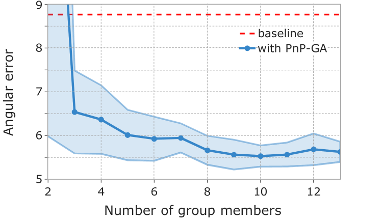
Figure 6: Evaluation of model adaptation performance with gradually increasing the number of group members.

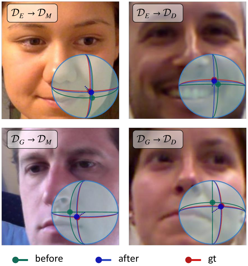
Figure 7: Visual results example of estimated 3D gaze. Red points represent the ground-truth gaze direction, green and blue points represent the predictions before and after adaptation, respectively.

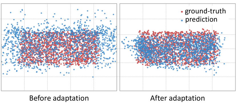
Figure 8: Scatter plot of predictions and ground-truth labels before and after model adaptation. Scatter points in blue represent predictions and red ones represent labels.

5.5 Comprehension of PnP-GA

To understand how our method improves the performance of gaze estimation in target domains, we 1) visualize typical cases by drawing gaze predictions on the input and 2) compare the prediction distributions before/after gaze domain adaptation. In detail, examples of visual gaze estimation results on four adaptation tasks are illustrated in Fig. 7. Results show that our proposed PnP-GA  can adapt well in different conditions. When the gaze direction deviates from the face direction, our method can also generate an accurate gaze direction (right bottom figure in Fig. 7).

Fig. 8 shows the distributions of predictions before and after adaptation. Our method significantly reduces the degree of outlier, the prediction distribution of our method are much closer to the distribution of ground-truth labels. These results also reveal that how our PnP-GA  improves the performance of gaze estimation.

6 Conclusion

In this paper we presented a novel outlier-guided plug-and-play gaze adaptation framework (PnP-GA) for generalizing the gaze estimation to new domains. The proposed PnP-GA  framework is model agnostic, in which most existing gaze estimation networks can be plugged without any modifications. Collaborative learning process and a novel outlier-guided loss are proposed for PnP-GA. Our method demonstrates superior performance on four gaze domain adaptation tasks, as well as exceptionally improved performance of plugging existing gaze estimation networks into the PnP-GA  framework.

References

- [1] Henny Admoni and Brian Scassellati. Social eye gaze in human-robot interaction: a review. Journal of Human-Robot Interaction, 6(1):25–63, 2017.
- [2] Alisa Burova, John Mäkelä, Jaakko Hakulinen, Tuuli Keskinen, Hanna Heinonen, Sanni Siltanen, and Markku Turunen. Utilizing vr and gaze tracking to develop ar solutions for industrial maintenance. In CHI, 2020.
- [3] Minjie Cai, Feng Lu, and Yoichi Sato. Generalizing hand segmentation in egocentric videos with uncertainty-guided model adaptation. In CVPR, 2020.
- [4] Nora Castner, Thomas C Kuebler, Katharina Scheiter, Juliane Richter, Thérése Eder, Fabian Hüttig, Constanze Keutel, and Enkelejda Kasneci. Deep semantic gaze embedding and scanpath comparison for expertise classification during opt viewing. In ACM Symposium on Eye Tracking Research and Applications, 2020.
- [5] Minghao Chen, Hongyang Xue, and Deng Cai. Domain adaptation for semantic segmentation with maximum squares loss. In ICCV, 2019.
- [6] Zhaokang Chen and Bertram E. Shi. Appearance-based gaze estimation using dilated-convolutions. In ACCV, 2018.
- [7] Yihua Cheng, Shiyao Huang, Fei Wang, Chen Qian, and Feng Lu. A coarse-to-fine adaptive network for appearance-based gaze estimation. In AAAI, 2020.
- [8] Shuhao Cui, Shuhui Wang, Junbao Zhuo, Chi Su, Qingming Huang, and Qi Tian. Gradually vanishing bridge for adversarial domain adaptation. In CVPR, pages 12455–12464, 2020.
- [9] Geoffrey French, Michal Mackiewicz, and Mark Fisher. Self-ensembling for visual domain adaptation. In ICLR, 2018.
- [10] Kenneth Alberto Funes Mora, Florent Monay, and Jean-Marc Odobez. Eyediap: A database for the development and evaluation of gaze estimation algorithms from rgb and rgb-d cameras. In ETRA, 2014.
- [11] Yixiao Ge, Dapeng Chen, and Hongsheng Li. Mutual mean-teaching: Pseudo label refinery for unsupervised domain adaptation on person re-identification. In ICLR, 2020.
- [12] Michael A Gerber, Ronald Schroeter, Li Xiaomeng, and Mohammed Elhenawy. Self-interruptions of non-driving related tasks in automated vehicles: Mobile vs head-up display. In CHI, 2020.
- [13] Ian J. Goodfellow, Jean Pouget-Abadie, Mehdi Mirza, Bing Xu, David Warde-Farley, Sherjil Ozair, Aaron Courville, and Yoshua Bengio. Generative adversarial nets. In NIPS, 2014.
- [14] Zidong Guo, Zejian Yuan, Chong Zhang, Wanchao Chi, Yonggen Ling, and Shenghao Zhang. Domain adaptation gaze estimation byembedding with prediction consistency. In ACCV(oral), 2020.
- [15] Kaiming He, Xiangyu Zhang adn Shaoqing Ren, and Jian Sun. Deep residual learning for image recognition. CVPR, 2016.
- [16] Kaiming He, Haoqi Fan, Yuxin Wu, Saining Xie, and Ross Girshick. Momentum contrast for unsupervised visual representation learning. arXiv preprint arXiv:1911.05722, 2019.
- [17] Judy Hoffman, Eric Tzeng, Jun-Yan Zhu Taesung Park, Phillip Isola, Kate Saenko, Alexei A. Efros, and Trevor Darrell. Cycada: Cycle-consistent adversarial domain adaptation. In CVPR, 2017.
- [18] Lu Jiang, Zhengyuan Zhou, Thomas Leung, Li-Jia Li, and Li Fei-Fei. Mentornet: Learning data-driven curriculum for very deep neural networks on corrupted labels. In ICML. PMLR, 2018.
- [19] Petr Kellnhofer, Adria Recasens, Simon Stent, Wojciech Matusik, and Antonio Torralba. Gaze360: Physically unconstrained gaze estimation in the wild. In ICCV, 2019.
- [20] Robert Konrad, Anastasios Angelopoulos, and Gordon Wetzstein. Gaze-contingent ocular parallax rendering for virtual reality. ACM Transactions on Graphics (TOG), 2020.
- [21] Felix Kuhnke and Jorn Ostermann. Deep head pose estimation using synthetic images and partial adversarial domain adaption for continuous label spaces. In ICCV, 2019.
- [22] Dong-Hyun Lee. Pseudo-label : The simple and efficient semi-supervised learning method for deep neural networks. In ICML, 2013.
- [23] Mingsheng Long, Zhangjie Cao, Jianmin Wang, and Michael I. Jordan. Conditional adversarial domain adaptation. In NIPS, 2018.
- [24] Feng Lu, Yusuke Sugano, Takahiro Okabe, and Yoichi Sato. Adaptive linear regression for appearance-based gaze estimation. In PAMI, 2014.
- [25] Seonwook Park, Shalini De Mello, Pavlo Molchanov, Umar Iqbal, Otmar Hilliges, and Jan Kautz. Few-shot adaptive gaze estimation. In ICCV, pages 9368–9377, 2019.
- [26] Ashish Shrivastava, Tomas Pfister, Oncel Tuzel, Josh Susskind, Wenda Wang, and Russ Webb. Learning from simulated and unsupervised images through adversarial training. In CVPR, 2017.
- [27] Antti Tarvainen and Harri Valpola. Mean teachers are better role models: Weight-averaged consistency targets improve semi-supervised deep learning results. In ICLR, 2017.
- [28] Yunus Terzioğlu, Bilge Mutlu, and Erol Şahin. Designing social cues for collaborative robots: the role of gaze and breathing in human-robot collaboration. In Proceedings of the 2020 ACM/IEEE International Conference on Human-Robot Interaction, 2020.
- [29] Eric Tzeng, Judy Hoffman, Kate Saenko, and Trevor Darrell. Adversarial discriminative domain adaptation. In CVPR, 2017.
- [30] Haofei Wang, Xujiong Dong, Zhaokang Chen, and Bertram E Shi. Hybrid gaze/eeg brain computer interface for robot arm control on a pick and place task. In 2015 37th Annual International Conference of the IEEE Engineering in Medicine and Biology Society (EMBC), pages 1476–1479. IEEE, 2015.
- [31] Kang Wang, Rui Zhao, Hui Su, and Qiang Ji. Generalizing eye tracking with bayesian adversarial learning. In CVPR, 2019.
- [32] Zhimin Wang, Huangyue Yu, Haofei Wang, Zongji Wang, and Feng Lu. Comparing single-modal and multimodal interaction in an augmented reality system. In ISMAR. IEEE, 2020.
- [33] Yu Yu, Gang Liu, and Jean-Marc Odobez. Improving few-shot user-specific gaze adaptation via gaze redirection synthesis. In CVPR, 2019.
- [34] Chiyuan Zhang, Samy Bengio, Moritz Hardt, Benjamin Recht, and Oriol Vinyals. Understanding deep learning requires rethinking generalization. In ICLR, 2017.
- [35] Xucong Zhang, Seonwook Park, Thabo Beeler, Derek Bradley, Siyu Tang, and Otmar Hilliges. Eth-xgaze: A large scale dataset for gaze estimation under extreme head pose and gaze variation. In ECCV. Springer, 2020.
- [36] Xucong Zhang, Yusuke Sugano, Mario Fritz, and Andreas Bulling. It’s written all over your face: Full-face appearance-based gaze estimation. In CVPR, 2017.
- [37] Xucong Zhang, Yusuke Sugano, Mario Fritz, and Andreas Bulling. Mpiigaze: Real-world dataset and deep appearance-based gaze estimation. PAMI, 2017.
- [38] Yabin Zhang, Hui Tang, Kui Jia, and Mingkui Tan. Domain-symmetric networks for adversarial domain adaptation. In CVPR, 2019.
- [39] Ying Zhang, Tao Xiang, Timothy M Hospedales, and Huchuan Lu. Deep mutual learning. In CVPR, 2018.
- [40] Yang Zou, Zhiding Yu, B. V. K. Vijaya Kumar, and Jinsong Wang. Domain adaptation for semantic segmentation via class-balanced self-training. In ECCV, 2018.