On the Angular Momentum Extraction from the Rotation Powered Pulsars

Abstract

The rotation powered pulsar loses angular momentum at a rate of the rotation power divided by the angular velocity $\Omega_{*}$. This means that the length of the lever arm of the angular momentum extracted by the photons, relativistic particles and wind must be on average $c/\Omega_{*}$, which is known as the light cylinder radius. Therefore, any deposition of the rotation power within the light cylinder causes insufficient loss of angular momentum. In this paper, we investigate two cases of this type of energy release: polar cap acceleration and Ohmic heating in the magnetospheric current inside the star. As for the first case, the outer magnetosphere beyond the light cylinder is found to compensate the insufficient loss of the angular momentum. We argue that the energy flux coming from the sub-rotating magnetic field lines must be larger than the solid-angle average value, and as a result, an enhanced energy flux emanating beyond the light cylinder is observed in different phases in the light curve from those of emission inside the light cylinder. As for the second case, the stellar surface rotates more slowly than the stellar interior. We find that the way the magnetospheric current closes inside the star is linked to how the angular momentum is transferred inside the star. We obtain numerical solutions which shows that the magnetospheric current inside the star spreads over the polar cap magnetic flux embedded in the star in such a way that electromotive force is gained efficiently.

1 Introduction

Rotation powered pulsars (RPPs), by definition, release rotational energy at a rate of $\dot{E}=-\Im\Omega_{*}\dot{\Omega}_{*}$, where $\Im$, $\Omega_{*}$, and $\dot{\Omega}_{*}$ are the moment of inertia, angular velocity and its time derivative of the neutron star. The associated angular momentum $\dot{L}=-\Im\dot{\Omega}_{*}$ is released at the same time. Therefore the ratio $\dot{E}/\dot{L}=\Omega_{*}$ is unique. This relation is usually not explicitly incorporated in theoretical modellings; it is justified on the basis of the fact that the relation is automatically satisfied as long as the system is solved self-consistently. In reality, however, the magnetosphere of RPPs is so complicated that no models have ever treated the whole system self-consistently. Instead, some specific part of the magnetosphere or neutron-star interior has been always a subject of theoretical modelling, and accordingly the relation between the energy and angular momentum $\dot{E}/\dot{L}=\Omega_{*}$ cannot be examined. Any of the past modelling works can be incompatible with the energy-angular-momentum relation. In this paper, we investigate two cases, the polar cap model and the current closure problem inside the neutron star with Ohmic dissipation, in which little angular momentum is lost.

As for the first case, the polar cap model, rotational energy is extracted through photons while hardly any angular momentum is carried off by these photons. Specifically when a curvature gamma-photon with energy $\epsilon$ is emitted from the polar caps, the angular momentum that it carries off is at most $\sim\epsilon R_{*}/c$, whereas the value implied by the energy-angular-momentum relation is $\epsilon/\Omega_{*}=\epsilon R_{L}/c$, where $R_{*}$ is the radius of the neutron star and $R_{L}=c/\Omega_{*}$ is the light cylinder radius, i.e., the favoured length of the lever arm is $R_{L}$, which is much larger than $R_{*}$. In terms of classical electromagnetism, it is worth noting that the wave zone of the magnetic dipole radiation originates around the light cylinder. In this case, the length of lever arm is $R_{L}$, regarding the wave front is not spherical but spirals in such a way that $\dot{E}/\dot{L}=\Omega_{*}$ holds. Since the energy-angular-momentum relation is required for the whole system, even if the polar caps do not emit sufficient angular momentum ($R_{*}\ll R_{L}$), a part of the outer magnetosphere must emit photons with a lever arm length larger than $R_{L}$ to compensate the insufficiency or equivalently electromagnetic waves are modified beyond the light cylinder. This may lead to a hypothesis that the polar cap emission will not make any significant effect on the magnetospheric structure. However, the observed radio luminosity becomes comparable with the spin-down luminosity for old pulsars (Wu et al., 2020). This fact implies that the polar cap luminosity can contribute to a significant fraction of $\dot{E}$, and that the inefficiency of the angular momentum loss may cause some crucial effect on the outer magnetosphere.

As for the second case, the Ohmic dissipation inside the star, the magnetospheric current goes out of and comes back to the star, thereby conveying the rotation energy of the star away through the magnetosphere. The magnetospheric current runs inside the star to make the circuit closed. This current generates the braking torque. Note that the term “magnetospheric current inside the star” does not include the current generated through the magneto-thermal evolution of the neutron star but means the current that is connected to the magnetosphere. If the Ohmic dissipation takes place on the magnetospheric current inside the star, a part of the rotational energy is converted to heat, which is eventually radiated away, while there is no loss of angular momentum from the system. This effect was not taken into account in the previous works of this subject (Beskin et al., 2015; Karageorgopoulos, Gourgouliatos & Contopoulos, 2019) which considered how the magnetospheric current ran inside the star.

In this paper, we investigate the above-mentioned two cases and discuss what would happen when the rotational energy is lost but not the angular momentum. Especially, for the second case, we demonstrate how the magnetospheric current inside the star is determined.

2 Basic relations

In this paper, we consider the obliquely rotating magnetosphere in a steady state. In this case, the electric field is written in the form of

$${\mbox{\boldmath$E$}}=-{1\over c}{\mbox{\boldmath$u$}_{\rm c}}\times{\mbox{\boldmath$B$}}-\nabla\Phi$$ (1)

without loss of generality (Mestel, 1999), where ${\mbox{\boldmath$u$}_{\rm c}}=\mbox{\boldmath$\Omega$}_{*}\times\mbox{\boldmath$r$}$ is the corotation vector, $B$ is the magnetic field, and $\Phi$ is a scalar potential called the “non-corotational electric potential”. The first term of the equation is the corotational electric field ${\mbox{\boldmath$E$}}_{\rm c}=-{\mbox{\boldmath$u$}_{\rm c}}\times{\mbox{\boldmath$B$}}/c$. The field-aligned electric field is given by $E_{\parallel}=-\hat{{\mbox{\boldmath$B$}}}\cdot\nabla\Phi$, where $\hat{{\mbox{\boldmath$B$}}}={\mbox{\boldmath$B$}}/|{\mbox{\boldmath$B$}}|$ is the unit vector along the magnetic field. Some useful formulae under the steadiness condition are given in the appendix.

Here let us assume at the moment that the star is a perfect conductor satisfying the ideal-magneto-hydrodynamic (MHD) condition, ${\mbox{\boldmath$E$}}+{\mbox{\boldmath$v$}}\times{\mbox{\boldmath$B$}}/c=0$, and rotates rigidly with ${\mbox{\boldmath$v$}}={\mbox{\boldmath$u$}_{\rm c}}$, where $v$ indicates the velocity field. Then the electric field is ${\mbox{\boldmath$E$}}_{\rm c}$ and $\Phi=\mbox{constant}=0$ inside the star. If the surrounding space is filled with plasma satisfying the ideal-MHD condition, then

$${1\over c}({\mbox{\boldmath$v$}}-{\mbox{\boldmath$u$}_{\rm c}})\times{\mbox{\boldmath$B$}}=\nabla\Phi$$ (2)

holds so that ${\mbox{\boldmath$B$}}\cdot\nabla\Phi=0$, meaning that the value $\Phi=0$ on the stellar surface propagates into the magnetosphere along $B$. Thus we have the corotation electric field and the iso-rotation

$${\mbox{\boldmath$v$}}={\mbox{\boldmath$u$}_{\rm c}}+\kappa{\mbox{\boldmath$B$}}$$ (3)

in the magnetosphere, where $\kappa$ is a scalar function.

The torque density in the star is given by $({\mbox{\boldmath$u$}_{\rm c}}/\Omega_{*})\cdot({\mbox{\boldmath$j$}}\times{\mbox{\boldmath$B$}}/c)$, and therefore the net torque on the star is

$$N={1\over\Omega_{*}}\int_{{\cal{V}}_{*}}{\mbox{\boldmath$u$}_{\rm c}}\cdot\left({1\over c}{\mbox{\boldmath$j$}}\times{\mbox{\boldmath$B$}}\right)\ dV={1\over\Omega_{*}}\int_{{\cal{V}}_{*}}{\mbox{\boldmath$E$}}_{\rm c}\cdot{\mbox{\boldmath$j$}}\ dV,$$ (4)

where $j$ is the current density of the magnetospheric current, and ${\cal{V}}_{*}$ is the stellar volume. The rotational power released from the star is thus given by $\Omega_{*}N$. The Poynting theorem

$${\partial U\over\partial t}+\nabla\cdot\mbox{\boldmath$S$}=-{\mbox{\boldmath$j$}}\cdot{\mbox{\boldmath$E$}}$$ (5)

where

$$U={E^{2}+B^{2}\over 4\pi},\ \ \ \mbox{\boldmath$S$}={c\over 4\pi}{\mbox{\boldmath$E$}}\times{\mbox{\boldmath$B$}},$$ (6)

reduces to

$$\nabla\cdot(\mbox{\boldmath$S$}-U{\mbox{\boldmath$u$}_{\rm c}})=-{\mbox{\boldmath$j$}}\cdot{\mbox{\boldmath$E$}}$$ (7)

in the steady condition. Combining (4) and (7) with the assumption ${\mbox{\boldmath$E$}}={\mbox{\boldmath$E$}}_{\rm c}$, we have the rotation power represented by the surface integral over the stellar surface ${{\cal{S}}}_{*}$:

$$\dot{E}=-\Omega_{*}N=\int_{{{\cal{S}}}_{*}}(\mbox{\boldmath$S$}-U{\mbox{\boldmath$u$}_{\rm c}})\cdot\ d{\mbox{\boldmath$A$}}.$$ (8)

This indicates that the rotational energy flowing out to the magnetosphere is accounted by the Poynting flux on the stellar surface.

3 Effect of the Polar Cap Accelerator on the Global Structure

We investigate the influence of the polar cap acceleration on the global torque balance of the magnetosphere.

We use a simple model as described below and illustrated in Fig. 1. Suppose a closed surface ${\cal{S}}$ surround the neutron star. The ideal-MHD condition is satisfied inside the surface ${\cal{S}}$ except for a particle-acceleration region along open field lines (the grey region in the figure). The region between ${\cal{S}}$ and ${{\cal{S}}}_{*}$ may be called the “inner magnetosphere”, provided that ${\cal{S}}$ is within the light cylinder. The region beyond ${\cal{S}}$ may be called the “outer magnetosphere”, where the ideal-MHD condition is assumed to hold. The outer magnetosphere possesses a field-aligned outflow, the pulsar wind.

Figure 1: A simple model of a magnetosphere with a field-aligned particle accelerator. Circular solid-line ${\cal{S}}_{*}$ is the stellar surface and the dashed-curve ${{\cal{S}}}$ is an arbitrary closed surface. Gray-shaded region indicates a particle-acceleration region.

Immediately above the stellar surface ${{\cal{S}}}_{*}$ and below the acceleration region, $\Phi=0$, ${\mbox{\boldmath$E$}}={\mbox{\boldmath$E$}}_{\rm c}$ and the flow obeys the relation ${\mbox{\boldmath$v$}}={\mbox{\boldmath$u$}_{\rm c}}+\kappa{\mbox{\boldmath$B$}}$. In the acceleration region, by contrast, there is a field-aligned electric field $E_{\parallel}=-\hat{{\mbox{\boldmath$B$}}}\cdot\nabla\Phi\not=0$. Even if the ideal-MHD condition is recovered beyond the acceleration region, variation of the non-corotational electric potential causes drift motions:

$${\mbox{\boldmath$v$}}={\mbox{\boldmath$u$}_{\rm c}}-{c{\mbox{\boldmath$B$}}\times\nabla\Phi\over B^{2}}+\kappa^{\prime}{\mbox{\boldmath$B$}}.$$ (9)

This may be attributed to the sub-pulse drift motion (Szary et al., 2020).

The equation of motion for the particles in the inner magnetosphere may be

$${1\over c}e_{\rm s}n_{\rm s}{\mbox{\boldmath$v$}}_{\rm s}\times{\mbox{\boldmath$B$}}+e_{\rm s}n_{\rm s}{\mbox{\boldmath$E$}}=n_{\rm s}\left({\partial\over\partial t}+{\mbox{\boldmath$v$}}_{\rm s}\cdot\nabla\right)(m_{\rm s}\gamma_{\rm s}{\mbox{\boldmath$v$}}_{\rm s})-\mbox{\boldmath$F$}_{\rm ext}$$ (10)

where $\mbox{\boldmath$F$}_{\rm ext}$ represents any non-electromagnetic forces, the subscript “s” indicates the particle species, and $e_{\rm s}$, $n_{\rm s}$, ${\mbox{\boldmath$v$}}_{\rm s}$, and $\gamma_{\rm s}$ are respectively the charge, number density, velocity, and the Lorentz factor. For the reaction force by the curvature radiation we have

$$\mbox{\boldmath$F$}_{\rm ext} = -{n_{\rm s}{\cal P}_{\rm s}\over c}{{\mbox{\boldmath$v$}}_{\rm s}\over c},$$ (11)

$${\cal P}_{\rm s} = (2e_{\rm s}^{2}/3c^{3})\gamma_{\rm s}^{4}|{\mbox{\boldmath$v$}}_{\rm s}\times(\nabla\times{\mbox{\boldmath$v$}}_{\rm s})|^{2}=(2e_{\rm s}^{2}c/3R_{\rm c}^{2})\gamma_{\rm s}^{4},$$ (12)

where $R_{\rm c}$ is the the radius of curvature. The work done by the electromagnetic force per unit time is given by the left-hand side of ${\mbox{\boldmath$v$}}_{\rm s}\cdot$(10) for each particle species, so that in total we have

$$\dot{E}_{\rm in}=\int_{{\cal{V}}_{\rm in}}\sum_{\rm s}{\mbox{\boldmath$v$}}_{\rm s}\cdot(e_{\rm s}n_{\rm s}{\mbox{\boldmath$E$}})dV=\int_{{\cal{V}}_{\rm in}}{\mbox{\boldmath$j$}}\cdot{\mbox{\boldmath$E$}}dV,$$ (13)

where ${\cal{V}}_{\rm in}$ indicates the volume between the surface ${\cal{S}}$ and ${{\cal{S}}}_{*}$. The value $\dot{E}_{\rm in}$ is the energy carried off by photons and/or particles from the inner magnetosphere.

The component along the rotation axis of the torque (the transferred angular momentum per unit time) is given by $({\mbox{\boldmath$u$}_{\rm c}}/\Omega_{*})\cdot$(10):

$$\dot{L}_{{\rm in}} = {1\over\Omega_{*}}\int_{{\cal{V}}_{\rm in}}\sum_{\rm s}{\mbox{\boldmath$u$}_{\rm c}}\cdot\left[{1\over c}e_{\rm s}n_{\rm s}{\mbox{\boldmath$v$}}_{\rm s}\times{\mbox{\boldmath$B$}}+e_{\rm s}n_{\rm s}{\mbox{\boldmath$E$}}\right]dV$$ (14)

$$= {1\over\Omega_{*}}\int_{{\cal{V}}_{\rm in}}({\mbox{\boldmath$j$}}\cdot{\mbox{\boldmath$E$}}+{\mbox{\boldmath$j$}}\cdot\nabla\Phi-q{\mbox{\boldmath$u$}_{\rm c}}\cdot\nabla\Phi)\ dV,$$ (15)

where (1) is used in the last manipulation and $q=\sum_{\rm s}e_{\rm s}n_{\rm s}$ is the charge density. Subtracting $\Omega_{*}$ times (15) from (13) yields

$$\Delta\dot{E}_{\rm in}\equiv\dot{E}_{\rm in}-\Omega_{*}\dot{L}_{\rm in} = -\int_{{\cal{V}}_{\rm in}}({\mbox{\boldmath$j$}}-q{\mbox{\boldmath$u$}_{\rm c}})\cdot\nabla\Phi\ dV$$ (16)

$$\approx \int_{{\cal{V}}_{\rm in}}j_{\parallel}E_{\parallel}\ dV\not=0,$$ (17)

where $j_{\parallel}={\mbox{\boldmath$j$}}\cdot\hat{{\mbox{\boldmath$B$}}}$, the approximation in the last step is based on the facts that the ratio of the microscopic to macroscopic time scales $|j_{\perp}/j_{\parallel}|=|{\mbox{\boldmath$j$}}\times\hat{{\mbox{\boldmath$B$}}}|/|{\mbox{\boldmath$j$}}\cdot\hat{{\mbox{\boldmath$B$}}}|\approx(c/R_{\rm c})/(e_{\rm s}B/\gamma_{\rm s}m_{\rm s}c)$ is negligible, and $|{\mbox{\boldmath$u$}_{\rm c}}|\ll c$ holds in the inner magnetosphere. The derived equation indicates that no significant amount of the angular momentum is lost from the inner magnetosphere.

In our simple model, the outer magnetosphere is treated in the one-fluid approximation with the ideal-MHD condition. The equation of motion is

$${1\over c}{\mbox{\boldmath$j$}}\times{\mbox{\boldmath$B$}}+q{\mbox{\boldmath$E$}} = n\left({\partial\over\partial t}+{\mbox{\boldmath$v$}}\cdot\nabla\right)(m\gamma{\mbox{\boldmath$v$}})$$ (18)

$$= n\left[{\partial m\gamma{\mbox{\boldmath$v$}}\over\partial t}+\nabla(mc^{2}\gamma)-{\mbox{\boldmath$v$}}\times(\nabla\times m\gamma{\mbox{\boldmath$v$}})\right].$$ (19)

From ${\mbox{\boldmath$v$}}\cdot$ (18) and $({\mbox{\boldmath$u$}_{\rm c}}/\Omega_{*})\cdot$ (18), it is straightforward to obtain the energy and angular momentum conservation laws:

$$\nabla\cdot\mbox{\boldmath$\cal E$}=0,\ \ \ \ \nabla\cdot\mbox{\boldmath$\cal L$}=0,$$ (20)

where

$$\cal E = mn\gamma c^{2}{\mbox{\boldmath$w$}}+\mbox{\boldmath$S$}-U{\mbox{\boldmath$u$}_{\rm c}},$$ (21)

$$\cal L = nm\gamma[({\mbox{\boldmath$u$}_{\rm c}}/\Omega_{*})\cdot{\mbox{\boldmath$v$}}]{\mbox{\boldmath$w$}}+(S-U{\mbox{\boldmath$u$}_{\rm c}})/\Omega_{*}-({\mbox{\boldmath$j$}}-q{\mbox{\boldmath$u$}_{\rm c}})(\Phi/\Omega_{*}),$$ (22)

where ${\mbox{\boldmath$w$}}={\mbox{\boldmath$v$}}-{\mbox{\boldmath$u$}_{\rm c}}$. The first terms of the expressions above are the contribution from the particles, while the last two terms are from the electromagnetic fields. The energy-angular momentum outflow through the surface ${\cal{S}}$ can be evaluated with the last two terms, namely

$$\dot{E}_{\rm out} = \int_{{\cal{S}}}(\mbox{\boldmath$S$}-U{\mbox{\boldmath$u$}_{\rm c}})\cdot d{\mbox{\boldmath$A$}},$$ (23)

$$\dot{L}_{\rm out} = {1\over\Omega_{*}}\int_{{{\cal{S}}}}(\mbox{\boldmath$S$}-U{\mbox{\boldmath$u$}_{\rm c}})\cdot d{\mbox{\boldmath$A$}}$$ (24)

$$+{1\over\Omega_{*}}\int_{{{\cal{S}}}}[({\mbox{\boldmath$j$}}-q{\mbox{\boldmath$u$}_{\rm c}})(-\Phi)]\cdot d{\mbox{\boldmath$A$}}.$$

These are used in part for the wind acceleration, and the unused parts of them propagate to the termination shock in a form of Poynting energy. As is expected, (23), (24) and (16) are combined to yield

$$\dot{E}_{\rm in}+\dot{E}_{\rm out}=\Omega_{*}(\dot{L}_{\rm in}+\dot{L}_{\rm out}).$$ (25)

The torque balance is satisfied in the whole system. Although we are not concerned with what actually happens in the outer magnetosphere, it is certain that the outer magnetosphere carries angular momentum so efficiently as to achieve the torque balance of the whole system. This fact together with the source of Poynting flux being provided by braking torque, (8), is included in classical electromagnetism (Beskin, 2010). If we define the effective angular velocity $\Omega_{\rm out}$ of the outer magnetosphere as $\Omega_{out}=\dot{E}_{\rm out}/\dot{L}_{\rm out}$, we obtain the relation

$$\Omega_{\rm out}=\Omega_{*}{1\over 1+\Delta\dot{E}_{\rm in}/\dot{E}_{\rm out}}<\Omega_{*}.$$ (26)

This indicates that the effective light-cylinder radius $c/\Omega_{\rm out}$ is larger than $R_{L}$. In other words, the lever arm of the angular momentum carried away from the outer magnetosphere becomes larger to compensate the inefficient angular momentum loss from the inner magnetosphere; the body inside the surface ${\cal{S}}$ is effectively a slow rotator. In this case, if photons are emitted in the outer magnetosphere, the emission site must be beyond the light cylinder. Alternatively, the Poynting vector in the wind would tilt to satisfy $|\mbox{\boldmath$r$}\times\mbox{\boldmath$S$}|/|\mbox{\boldmath$S$}|>R_{L}$. What exactly happens in the outer magnetosphere is discussed in §6.

4 Effect of Ohmic Heating on the Torque Balance of the Star Interior

If Ohmic dissipation is present on the magnetospheric current which makes a circuit inside the star, then rotational energy is consumed without any loss of angular momentum. Let us consider this case in this section.

For the present discussion we employ a two-component (proton-electron) plasma with frictional force. The equations of motion can be written as

$$m_{\rm p}n_{\rm p}{{\rm D}{\mbox{\boldmath$v$}}_{\rm p}\over{\rm D}t} = en_{\rm p}{\mbox{\boldmath$E$}}+{1\over c}en_{\rm p}{\mbox{\boldmath$v$}}_{\rm p}\times{\mbox{\boldmath$B$}}+\mbox{\boldmath$F$}_{\rm f},$$ (27)

$$m_{\rm e}n_{\rm e}{{\rm D}{\mbox{\boldmath$v$}}_{\rm e}\over{\rm D}t} = -en_{\rm e}{\mbox{\boldmath$E$}}-{1\over c}en_{\rm e}{\mbox{\boldmath$v$}}_{\rm e}\times{\mbox{\boldmath$B$}}-\mbox{\boldmath$F$}_{\rm f},$$ (28)

where the left-hand sides represent the Lagrangian time derivative, the subscripts indicate the particle species, and $\mbox{\boldmath$F$}_{\rm f}$ is the frictional force which is given by

$$\mbox{\boldmath$F$}_{\rm f}=-m_{\rm e}n_{\rm e}({\mbox{\boldmath$v$}}_{\rm p}-{\mbox{\boldmath$v$}}_{\rm e})\nu_{\rm coll},$$ (29)

where $\nu_{\rm coll}$ is the effective collision frequency. A set of equations (27) and (28) is reduced to a familiar set of the one-fluid equation of motion and Ohm’s law:

$$m_{\rm p}n_{\rm p}{{\rm D}{\mbox{\boldmath$v$}}\over{\rm D}t} = q{\mbox{\boldmath$E$}}+{1\over c}{\mbox{\boldmath$j$}}\times{\mbox{\boldmath$B$}},$$ (30)

$${\mbox{\boldmath$E$}}+{1\over c}{\mbox{\boldmath$v$}}\times{\mbox{\boldmath$B$}} = {{\mbox{\boldmath$j$}}\over\sigma},$$ (31)

where the electric conductivity $\sigma=e^{2}n_{\rm e}/m_{\rm e}\nu_{\rm coll}$ is introduced and the approximation is based on ${\mbox{\boldmath$v$}}=(m_{\rm p}n_{\rm p}{\mbox{\boldmath$v$}}_{\rm p}+m_{\rm e}n_{\rm e}{\mbox{\boldmath$v$}}_{\rm e})/(m_{\rm p}n_{\rm p}+m_{\rm e}n_{\rm e})\approx{\mbox{\boldmath$v$}}_{\rm p}$, $q=e(n_{\rm p}-n_{\rm e})$, ${\mbox{\boldmath$j$}}=e(n_{\rm p}{\mbox{\boldmath$v$}}_{\rm p}-n_{\rm e}{\mbox{\boldmath$v$}}_{\rm e})$ and $q/en_{e}\ll 1$, whereas we ignore the Hall term, which is very small for the magnetospheric current (see § 6.2 for discussion). Using Ohm’s law is equivalent to using the two-component model with friction.

For the energy conservation, adding (27)$\cdot{\mbox{\boldmath$v$}}_{\rm p}$ and (28)$\cdot{\mbox{\boldmath$v$}}_{\rm e}$, we have

$$m_{\rm p}n_{\rm p}{{\rm D}{\mbox{\boldmath$v$}}_{\rm p}\over{\rm D}t}\cdot{\mbox{\boldmath$v$}}_{\rm p}+m_{\rm e}n_{\rm e}{{\rm D}{\mbox{\boldmath$v$}}_{\rm e}\over{\rm D}t}\cdot{\mbox{\boldmath$v$}}_{\rm e} = {\mbox{\boldmath$j$}}\cdot{\mbox{\boldmath$E$}}+({\mbox{\boldmath$v$}}_{\rm p}-{\mbox{\boldmath$v$}}_{\rm e})\cdot\mbox{\boldmath$F$}_{\rm f}$$ (32)

$$= {\mbox{\boldmath$j$}}\cdot{\mbox{\boldmath$E$}}-j^{2}/\sigma,$$

where the quasi-neutrality condition $n_{e}=n_{p}$ has been applied, and ${\mbox{\boldmath$j$}}=en_{\rm e}({\mbox{\boldmath$v$}}_{\rm p}-{\mbox{\boldmath$v$}}_{\rm e})$ in the last manipulation. Here we are concerned with only the rotational motion and set ${\mbox{\boldmath$v$}}_{\rm p}=\Omega r\mbox{\boldmath$e$}_{\varphi}$, where $r$ is the distance from the rotation axis and $\Omega$ is the angular velocity as a function of the position, whereas $\Omega_{*}$ is used for the angular velocity on the stellar surface. We should note that $\Omega_{*}$ determines the ratio of the energy and the angular momentum which flows out from the star. Ignoring the electron inertia, we obtain

$$\Omega\dot{\Omega}m_{\rm p}n_{\rm p}r^{2}={\mbox{\boldmath$j$}}\cdot{\mbox{\boldmath$E$}}-j^{2}/\sigma.$$ (33)

This is integrated over the volume of the star to give

$$\langle\Omega\dot{\Omega}\rangle\Im=\int_{{\cal{V}}_{*}}{\mbox{\boldmath$j$}}\cdot{\mbox{\boldmath$E$}}\ dV-\int_{{\cal{V}}_{*}}(j^{2}/\sigma)\ dV,$$ (34)

where

$$\Im=\int_{{\cal{V}}_{*}}m_{\rm p}n_{\rm p}r^{2}\ dV$$ (35)

is the moment of inertia of the star, and the operator $\langle\ \rangle$ indicates taking the average. Equation (34) implies that some part of the rotational energy goes into Joule heating and the rest is the source of the Poynting flux which flows into the magnetosphere; the volume integral of ${\mbox{\boldmath$j$}}\cdot{\mbox{\boldmath$E$}}$ is the surface integral of $S$ on the stellar surface (equations (4) and (8)).

As for the component along the rotation axis of the angular momentum, adding (27)$\cdot({\mbox{\boldmath$u$}_{\rm c}}/\Omega_{*})$ and (28)$\cdot({\mbox{\boldmath$u$}_{\rm c}}/\Omega_{*})$, we have

$$r\mbox{\boldmath$e$}_{\varphi}\cdot\left(m_{\rm p}n_{\rm p}{{\rm D}{\mbox{\boldmath$v$}}_{\rm p}\over{\rm D}t}+m_{\rm e}n_{\rm e}{{\rm D}{\mbox{\boldmath$v$}}_{\rm e}\over{\rm D}t}\right)={1\over\Omega_{*}}\left[q{\mbox{\boldmath$u$}_{\rm c}}\cdot{\mbox{\boldmath$E$}}+{1\over c}({\mbox{\boldmath$j$}}\times{\mbox{\boldmath$B$}})\cdot{\mbox{\boldmath$u$}_{\rm c}}\right],$$ (36)

where the frictional terms cancel each other out, following the action-reaction principle, and the Ohmic term has no effect on the angular momentum. Equation (36) is rewritten as, with ${\mbox{\boldmath$E$}}=-{\mbox{\boldmath$u$}_{\rm c}}\times{\mbox{\boldmath$B$}}/c-\nabla\Phi$ and $\nabla\cdot({\mbox{\boldmath$j$}}-q{\mbox{\boldmath$u$}_{\rm c}})=0$,

$$r\mbox{\boldmath$e$}_{\varphi}\cdot\left(m_{\rm p}n_{\rm p}{{\rm D}{\mbox{\boldmath$v$}}_{\rm p}\over{\rm D}t}+m_{\rm e}n_{\rm e}{{\rm D}{\mbox{\boldmath$v$}}_{\rm e}\over{\rm D}t}\right) = {1\over\Omega_{*}}\left[{\mbox{\boldmath$j$}}\cdot{\mbox{\boldmath$E$}}+(\nabla\Phi)\cdot({\mbox{\boldmath$j$}}-q{\mbox{\boldmath$u$}_{\rm c}})\right]$$ (37)

$$= {1\over\Omega_{*}}\left[{\mbox{\boldmath$j$}}\cdot{\mbox{\boldmath$E$}}+\nabla\cdot\{({\mbox{\boldmath$j$}}-q{\mbox{\boldmath$u$}_{\rm c}})\Phi\}\right].$$

The second term of the right-hand side is integrated over the star to give zero because $\Phi=0$ on the surface of the star:

$$\int_{{\cal{V}}_{*}}\nabla\cdot\{({\mbox{\boldmath$j$}}-q{\mbox{\boldmath$u$}_{\rm c}})\Phi\}dV=\int_{{{\cal{S}}}_{*}}({\mbox{\boldmath$j$}}-q{\mbox{\boldmath$u$}_{\rm c}})\Phi\cdot d{\mbox{\boldmath$A$}}=0.$$ (38)

Consequently, we obtain

$$\langle\dot{\Omega}\rangle\Im={1\over\Omega_{*}}\int_{{\cal{V}}_{*}}{\mbox{\boldmath$j$}}\cdot{\mbox{\boldmath$E$}}\ dV.$$ (39)

This means that all the lost angular momentum goes into the magnetosphere.

The ratio of the net losses of the energy and angular momentum is calculated to be

$$\langle\Omega\rangle\equiv{-\Im\langle\Omega\dot{\Omega}\rangle\over-\Im\langle\dot{\Omega}\rangle}=\Omega_{*}\left(1+{\int_{{\cal{V}}_{*}}(j^{2}/\sigma)dV\over\int_{{\cal{S}}_{*}}(\mbox{\boldmath$S$}-U{\mbox{\boldmath$u$}_{\rm c}})\cdot d\mbox{\boldmath$A$}}\right)>\Omega_{*}.$$ (40)

Therefore, the stellar interior rotates faster than the surface when Ohmic dissipation takes place. The main conclusion of this section is that in determining the magnetospheric current inside the star one must treat the dynamics of the interior matter, particularly the angular momentum transfer.

5 Distribution of the electric current Inside the Star

In the previous section, we have found that the magnetospheric current inside the star is determined not by Ohm’s law but by magneto-hydrodynamics. An illustrative example is given in this section.

Since Ohmic dissipation is very small in reality, the ideal-MHD condition may be appropriate in the stellar interior. In this case, we need not consider the differential rotation caused by Ohmic heating . In the following discussion we assume the rigid rotation in the form of ${\mbox{\boldmath$v$}}=\mbox{\boldmath$r$}\times\Omega(t)\mbox{\boldmath$e$}_{z}$. The basic equations are

$$\rho{D{\mbox{\boldmath$v$}}\over Dt} = {1\over c}{\mbox{\boldmath$j$}}\times{\mbox{\boldmath$B$}}-\nabla\mbox{\boldmath$\Pi$}-\nabla\Phi_{g},$$ (41)

$${\mbox{\boldmath$E$}}+{1\over c}{\mbox{\boldmath$v$}}\times{\mbox{\boldmath$B$}} = 0,$$ (42)

where $\rho$ is the mass density, $\Phi_{g}$ is the gravitational potential, and $\Pi$ is the stress tensor. The magnetic field $B$ and the associated current $j$ include the components that are “intrinsic” to the star, i.e., those determined from the star structure and evolution. We write them in the from of the intrinsic term plus the magnetospheric term: ${\mbox{\boldmath$B$}}={\mbox{\boldmath$B$}}_{0}+{\mbox{\boldmath$B$}}^{\prime}$ and ${\mbox{\boldmath$j$}}={\mbox{\boldmath$j$}}_{0}+{\mbox{\boldmath$j$}}^{\prime}$. The expansion is

$${\mbox{\boldmath$j$}}\times{\mbox{\boldmath$B$}}={\mbox{\boldmath$j$}}_{0}\times{\mbox{\boldmath$B$}}_{0}+{\mbox{\boldmath$j$}}^{\prime}\times{\mbox{\boldmath$B$}}_{0}+{\mbox{\boldmath$j$}}_{0}\times{\mbox{\boldmath$B$}}^{\prime}+{\mbox{\boldmath$j$}}^{\prime}\times{\mbox{\boldmath$B$}}^{\prime}.$$ (43)

Note that the the magnetospheric components are much smaller than the intrinsic ones ($|{\mbox{\boldmath$B$}}^{\prime}|/|{\mbox{\boldmath$B$}}_{0}|\sim(R_{*}/R_{L})^{3/2}$). The first term ${\mbox{\boldmath$j$}}_{0}\times{\mbox{\boldmath$B$}}_{0}/c$ is not related to the spin-down. The dominant braking force is due to the term ${\mbox{\boldmath$j$}}^{\prime}\times{\mbox{\boldmath$B$}}_{0}/c$. For the axisymmetric cases, this term is the only force in the azimuthal direction. We ignore the last term.

Because we have specified the velocity field in terms of $\Omega(t)$ and have introduced elasticity, the set of equations (41) and (42) have a solution for any given magnetospheric current ${\mbox{\boldmath$j$}}^{\prime}$. Then we cannot find a unique solution for the magnetospheric current distribution. However, if the stress is very high, the material will have viscous motion and/or cracks to reduce the elastic energy $E_{\rm el}$. The spin-down torque is too small to break the latices. Hence, minimization of $E_{\rm el}$ will be achieved only through tiny non-elastic change in the material, and thus the current distribution will change to the state in which $E_{\rm el}$ is minimized. We take the following steps: (i) solving (41) for a trial ${\mbox{\boldmath$j$}}^{\prime}$, (ii) calculating $E_{\rm el}$ from the obtained displacement $u_{\varphi}$, (iii) varying ${\mbox{\boldmath$j$}}^{\prime}$ and then recalculating $E_{\rm el}$, and (iv) finding ${\mbox{\boldmath$j$}}^{\prime}$ in the searched parameter space so as to minimize $E_{\rm el}$.

For simplicity, we assume axisymmetry about and uniform background magnetic fields along the rotation axis, ${\mbox{\boldmath$B$}}_{0}=B_{0}\mbox{\boldmath$e$}_{z}$. The star is assumed to be a uniform elastic body. The azimuthal component of the equation of motion is

$${\partial^{2}u_{\varphi}\over\partial{r}^{2}}+{1\over r}{\partial u_{\varphi}\over\partial r}-{u_{\varphi}\over r^{2}}+{\partial^{2}u_{\varphi}\over\partial{z}^{2}}+{F_{\varphi}-\rho\dot{\Omega}r\over\mu_{\rm s}}=0,$$ (44)

where we use the cylindrical coordinates $(r,\varphi,z)$, for which the unit vectors are denoted by $\mbox{\boldmath$e$}_{r}$, $\mbox{\boldmath$e$}_{\varphi}$ and $\mbox{\boldmath$e$}_{z}$, $u_{\varphi}$ is the displacement in the azimuthal direction, $F_{\varphi}=({\mbox{\boldmath$j$}}^{\prime}\times{\mbox{\boldmath$B$}}_{0})\cdot\mbox{\boldmath$e$}_{\varphi}/c$ is the electromagnetic force generated by the magnetospheric current, and $\mu_{\rm s}$ is the shear modulus which is uniform. We may use the spherical polar coordinates $(R,\theta,\varphi)$ occasionally.

The magnetospheric current inside the star is purely poloidal and is represented by, with the use of the current stream function $I=rB^{\prime}_{\varphi}c/2$,

$${\mbox{\boldmath$j$}}^{\prime}_{p}=-{c\over 4\pi r}\mbox{\boldmath$e$}_{\varphi}\times\nabla(rB^{\prime}_{\varphi})=-{1\over 2\pi r}\mbox{\boldmath$e$}_{\varphi}\times\nabla I.$$ (45)

It is notable that the contours of $I$ give the stream lines of the current. The value of $I$ on the star surface is denoted by $I_{*}(s)$, which is a function of the arc length from the pole along the meridian $s=R_{*}\theta$. The function $I_{*}(s)$ is treated as the boundary condition of the present model, connecting the star and magnetosphere. Note that $I_{*}(s)$ gives the net current running through the surface area with an angular range of $0\leq\theta\leq s/R_{*}$.

The azimuthal component of the electromagnetic force is

$$F_{\varphi}={1\over c}({\mbox{\boldmath$j$}}^{\prime}_{p}\times{\mbox{\boldmath$B$}}_{0})\cdot\mbox{\boldmath$e$}_{\varphi}={1\over 2\pi cr}{\mbox{\boldmath$B$}}_{0}\cdot\nabla I.$$ (46)

The net torque on the star is straightforwardly obtained with surface integration to be

$$N=\int_{{\cal{V}}_{*}}rF_{\varphi}dV={1\over 2\pi c}\int_{{\cal{S}}_{*}}I_{*}(s)\ {\mbox{\boldmath$B$}}_{0}\cdot d{\mbox{\boldmath$A$}}.$$ (47)

Once $I_{*}(s)$ has been given as a boundary condition, $\dot{\Omega}=N/\Im$ is determined.

The shear stress is given by

$$\Pi_{z\theta} = -\mu_{\rm s}{\partial u_{\varphi}\over\partial z},$$ (48)

$$\Pi_{r\theta} = -\mu_{\rm s}\left({\partial u_{\varphi}\over\partial r}-{u_{\varphi}\over r}\right).$$ (49)

The elastic energy is

$$E_{el}=\int_{{\cal{V}}_{*}}{\Pi_{z\theta}^{2}+\Pi_{r\theta}^{2}\over\mu_{\rm s}}dV.$$ (50)

If $I$ is specified, (44) is easily solved numerically, and the elastic energy is obtained.

We need to provide some trial current function. In this study, we employ for it simple cubic forms with a few parameters, which are determined so that $E_{\rm el}$ is minimized. For $I_{*}(s)$, a simple analytic function

$$I_{*}(s)=\left\{\begin{array}[]{lc}\displaystyle I_{0}\ {27\over 4}{s^{2}(s-s_{\rm pc})\over s_{\rm pc}^{3}}&\mbox{if }s<s_{\rm pc}\\ 0&\mbox{if }s>s_{\rm pc}\end{array}\right.$$ (51)

is assumed, where $s_{\rm pc}=R_{*}\theta_{\rm pc}$ with the polar cap co-latitude $\theta_{\rm pc}=\sqrt{R_{*}\Omega_{*}/c}$ (Fig. 2), and $I_{0}$ is the peak value, meaning the total circulating current. In the following numerical illustration , we use a slightly large value of $\theta_{\rm pc}=(R_{L}/R_{*})^{-1/2}=0.2913$ (corresponding to a 1-msec pulsar) to reduce numerical load. The current function within the star $I(r,z)$ describes how current runs inside the star. We additionally introduce a simple cubic function $K$ with the parameter $z_{2}$ above which one half of the current $I_{0}$ closes:

$${K}(\zeta)=\zeta^{2}(3-2\zeta)$$ (52)

with

$$\zeta(z) = \left(z\over z_{\rm surf}\right)^{1/\alpha},$$ (53)

$$\alpha = -{\log_{2}z_{2}},$$ (54)

where $z_{\rm surf}=\sqrt{R_{*}^{2}-r^{2}}$ is the $z$-value on the surface for a given $r$ (right panel of Fig. 2). Note that ${K}(0)=0$, ${K}(1/2)=1/2$, ${K}(1)=1$, and ${K}(\zeta(z=z_{2}))=1/2$.

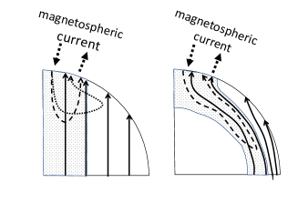
Figure 2: (Left panel) Current function $I_{*}(s)$ (Equation (52)) for the surface boundary, where $s$ and $I_{*}$ are in units of $R_{*}$ and $I_{0}$, respectively. (Right panel) Distribution $K(z)$ (Equation (53)right panel) as a function of $z$.

Although how deep the magnetospheric current penetrates into the star is parameterized by $z_{2}$, one may need to restrict the current in a layer $R_{1}<R<R_{*}$, say the crust. If this is the case, we use a diminishing factor of the Fermi-Dirac type:

$$K_{\rm cut}(R)={1\over\exp[(R_{1}-R)/\Delta R]+1},$$ (55)

where $\Delta R$ is the thickness for the transition. If not, $K_{\rm cut}=1$. Incorporating this factor $K_{\rm cut}$, we have

$$I(r,z)=K_{\rm cut}(R)\ K(\zeta(z))\ I_{*}(s(r)),$$ (56)

where $R=\sqrt{r^{2}+z^{2}}$, and $s=R_{*}\arcsin(r/R_{*})$. Some examples of $I(r,z)$ are shown in Fig. 3. As $z_{2}$ is decreased (see panels (a), (b) and (c), of Fig. 3 in this order), the current runs deeper along the field lines. If the diminishing factor is applied, the current is restricted above $R_{1}$ (panel (d)).

(a) (b)

(c) (d)

Figure 3: Contour maps of the current function $I(r,z)$ (Equation (56) ) with (a) $z_{2}=0.7z_{\rm surf}$, (b) $z_{2}=0.5z_{\rm surf}$, and (c) $z_{2}=0.3z_{\rm surf}$, without a diminishing factor, and (d) $z_{2}=0.5z_{\rm surf}$ with a diminishing factor $K_{\rm cut}(R)$ (Equation(55)) applied with $R_{1}=0.8R_{*}$ and $\Delta R=0.05R_{*}$. The coordinates are in units of $R_{*}$.

For the given current, we calculate $F_{\varphi}$ and $\dot{\Omega}$ from (46) and (47). Fig. 4(a) shows the shear moment $(F_{\varphi}-\rho\dot{\Omega}r)r^{2}$ for the case of $z_{2}=0.5z_{\rm surf}$. It shows that the inertial force in $+\varphi$ direction dominates in the equatorial region, whereas the electromagnetic braking force in $-\varphi$ direction does in the region $0\leq r\leq R_{*}\sin\theta_{\rm pc}$, which is the polar cap magnetic flux.

With the specified $F_{\varphi}$ and $\dot{\Omega}$, we solve (44) numerically to obtain the displacement $u_{\varphi}$. The obtained displacement is shows in Fig. 4(b). As is expected, the inner ($r\la 0.5$) and outer ( $r\ga 0.5$) regions are deformed in $+\varphi$ and $-\varphi$ directions, respectively. In the boundary region between the two, the elastic energy is large as shown in Fig. 4(c). The numerical calculation is done in the non-dimensional form, where all the formulae are the same except $c=1$. The force density, displacement and $E_{\rm el}$ are respectively in units of $F_{0}=B_{0}I_{0}/cR_{*}^{2}$, $F_{0}R_{*}^{2}/\mu_{\rm s}$, and $\dot{E}_{0}\Omega_{*}^{-1}$, where the unit of the power is $\dot{E}_{0}=(\mu_{\rm m}^{2}\Omega_{*}^{4}/c^{3})(2R_{L}/R_{*})$, and $\mu_{\rm m}$ is the magnetic moment of the star.

(a) (b)

(c)

Figure 4: (a) Distribution of force represented by the shear moment, (b) obtained displacement $u_{\varphi}$, and (c) elastic energy density for the case of $z_{2}=0.5z_{\rm surf}$ (Fig. 3(b)). The shear moment, displacement and $E_{\rm el}$ are in units of $F_{0}R_{*}^{2}$, $F_{0}R_{*}^{2}/\mu_{\rm s}$, and $\dot{E}_{0}\Omega_{*}^{-1}$,respectively.

We then obtain a series of solutions for different $z_{2}$ and find that the elastic energy is minimized at $z_{2}\sim 0.4z_{\rm surf}$ as shown in Fig. 5(a). This result is plausible, i.e., the elastic energy is decreased if the braking force is distributed over the whole neutron star to diminish the inertial force. Conversely, if the braking force is localized in a small region near the surface region ($z_{2}\sim 1$) or the core region ($z_{2}\sim 0$), then the elastic energy is increased. If the current is restricted in a layer above $R_{1}$, the thinner the current is restricted, the larger the elastic energy is (Fig. 5(b)).

In addition to this, if the current penetrates out of the polar cap magnetic flux tube ($r>R_{*}\sin\theta_{\rm pc}$), the electromagnetic force works in the opposite direction to the braking force ($+\varphi$ direction), and the elastic energy increases. As a result, the magnetospheric current inside the star is restricted in the polar cap magnetic flux tube. Thus, the configuration of ${\mbox{\boldmath$B$}}_{0}$, especially that of the polar cap magnetic flux plays essential role to relax the elastic energy of the star. This point is discussed in § 6.2.

(a) (b)

Figure 5: Total elastic energy as a function of (a) $z_{2}/z_{\rm surf}$ with $K_{\rm cut}=1$ and (b) $R_{1}$ with the fixed $z_{2}=0.5z_{\rm surf}$.

6 Discussion

6.1 Outer magnetosphere

The angular momentum extracted from the neutron star must be the rotation power divided by the angular velocity, $\dot{L}=\dot{E}/\Omega_{*}$. However, the polar cap accelerator emits a part of the rotational energy but emits little angular momentum. We have shown in § 3 that the inefficient loss of angular momentum is compensated by efficient loss of angular momentum in the outer magnetosphere beyond the light cylinder. The surface ${\cal{S}}$ in our simple model (Fig. 1) is effectively a slow rotator. Since the efficiency depends on $\Omega_{out}^{-1}=\dot{L}_{\rm out}/\dot{E}_{\rm out}$, a slower rotation than $\Omega_{*}$ (sub-rotation) plays a key role. This effect is more significant for older pulsars, for which the polar cap accelerator carries off an major fraction of the rotation power.

Let us consider what actually happens in the outer magnetosphere. The outer gap around the null surface is located within the light cylinder (Holloway, 1973) and therefore cannot account for the expected loss of the angular momentum. The polar cap accelerator and outer gap causes gradients of the non-corotational potential $\Phi$. As a result, the regions outside these accelerators show the sub-rotation and the super-rotation by the non-corotational drift motion according to (9). Fig. 6 illustrates the drift motion in the case of a nearly aligned rotator.

Figure 6: Field-aligned particle acceleration results in sub-rotation and super-rotation regions along field lines piercing field-aligned accelerators. The sub-rotating magnetic fluxes contribute to the efficient loss of angular momentum. The non-corotational potential $\Phi$ is zero everywhere except for the shaded regions. It is notable that the dotted regions satisfy the ideal-MHD condition but has the gradient of $\Phi$.

We argue that the energy is conveyed off efficiently along the sub-rotating open field lines to compensate the insufficient loss of angular momentum.

The emission beyond the light cylinder might be essential. Uzdensky (2003) showed that the ideal-MHD condition breaks down beyond the Y-point, the open-close boundary on the light cylinder. He showed that a wedge shaped region beyond the Y-point is electric field dominant, $|E|>|B|$, and the force-free approximation is no longer applicable there. This region indeed appears in particle simulations (Wada & Shibata, 2011; Yuki & Shibata, 2012). It has been suggested that the location of the Y-point is a free parameter for the force-free model (Timokhin, 2006). This fact alone might indicate that the Y-point shift outward so that the lever arm becomes larger than the light cylinder radius. However, as was suggested by Holloway (1973) and seen in Fig. 6 as well as in the numerical simulation (Wada & Shibata, 2011; Yuki & Shibata, 2012), the region around the open-close boundary is super-corotation, and hence the Y-point shifts inwards. The particle acceleration and radiation in the vicinity of the Y-point will not contribute to the efficient loss of the angular momentum, but the current sheet beyond the light cylinder will do. Some indication may be found in numerical simulations (e.g., (Brambilla et al., 2018)).

The compensation is not always associated with particle acceleration and subsequent radiation. It can be made in a form of a Poynting dominant wind, where the required condition would be $|\mbox{\boldmath$r$}\times\mbox{\boldmath$S$}|/|\mbox{\boldmath$S$}|>R_{L}$. Fig. 7 left panel shows the face-on view of the wind region with spiralling magnetic field lines. The pitch angle of the field lines is $\psi=c/\Omega_{*}r\ll 1$ at large distances on average. This is due to the fact that every quantity should have the pattern velocity $\Omega_{*}$ in steady state. However, some part can have a larger pitch angle than the average, and if so, the Poynting vector has a larger lever arm than the light-cylinder radius. Therefore, if the wind energy is concentrated in the part with such a large pitch angle, the Poynting dominant wind conveys a larger amount of the angular momentum than the value of the wind power divided by $\Omega_{*}$. In this case, the energy flux is not uniform with respect to the azimuthal angle, which implies that the pulsar wind has amplitude modulation. It is plausible that emission beyond the light cylinder may be observed out of the phase of the polar cap emission as shown in the right panel of Fig. 7.

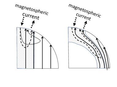
Figure 7: (Left panel) Face-on view of the field lines in the wind region. The larger the pitch angle of spiralling magnetic fields is, the larger the lever arm is, and the more efficient the angular momentum loss is. The average pitch angle must be $c/\Omega_{*}r$ (the thin spiral curve). In some phase angles as long as the system maintains the steady state. the pitch angle must be larger than the average value to carry a larger amount of angular momentum. (Right panel) a large amount of energy may reside out of the phase in which the polar caps emit.

6.2 Magnetospheric current inside the star

Ohmic dissipation of the magnetospheric current inside the star converts the rotation energy into heat, which is eventually radiated away. No angular momentum is lost in this process. We have shown that the Ohmic heating results in different angular velocities between the surface and interior of the star. Consequently the way the magnetospheric current inside the star closes is coupled with the angular momentum transfer in the star and accordingly cannot be solved solely by Ohm’s law, as erroneously done in Karageorgopoulos, Gourgouliatos & Contopoulos (2019).

In fact, the Ohmic heating is very small; the heating rate is given by $H\approx(j^{2}/\sigma)V$, where $V\approx\varepsilon R_{\rm pc}^{2}R_{*}$ is the volume and $\varepsilon$ is a numerical factor. Using $j\approx I_{0}/R_{\rm pc}^{2}$ and $\dot{E}\approx I_{0}^{2}/c$, we have

$$H=\dot{E}\left(R_{L}\over R_{*}\right)^{2}{\varepsilon\Omega\over\sigma}.$$ (57)

Adopting a typical value $\sigma\sim 10^{25}$ s^-1 (Chamel & Haensel, 2008), we have $H/\dot{E}=1.4\times 10^{-17}(\varepsilon P/1\mbox{s})$, where $P$ is the rotation period. The lack of the angular momentum release accumulates with time; e.g., in a month, $\Delta t\sim 10^{6}$ s, $H\Delta t/\Im\Omega^{2}$ $=\Delta\Omega/\Omega\sim 4\times 10^{-11}(\varepsilon P/1\mbox{s})$. This indicates that the insufficient loss cased by Ohmic heating contribute to some kinds of timing irregularities, such as glitches or some timing noises. But they are small as compared with the observed limit (Fuentes et al., 2017).

We have given an illustrative example for the case the ideal-MHD condition holds (no Ohmic loss) and the star is an elastic solid body in § 5. The current is determined in such a way that the elastic energy is minimized. As demonstrated by the numerical solution, the elastic energy is minimized when the current spreads over within the polar cap magnetic flux. In fact, if the elastic energy is high, the situation is relaxed due to small non-elastic changes or viscous motions and the current distribution is varied to reduce the elastic energy. In contrast to the Ohmic law, where the current tries to find a short cut (Beskin et al., 2015; Karageorgopoulos, Gourgouliatos & Contopoulos, 2019), the actual current distribution is determined in such a way that electromotive force is gained as efficiently as possible with least stress, and thus the current spreads over the stellar volume.

If the magnetic flux is uniform as is assumed in our numerical example, the current is distributed as shown in Fig. 3 (b) and the dashed curve in the left panel of Fig. 8. The current does not penetrate outside the polar magnetic flux; if it did, the electromagnetic force would be in opposite direction to the braking force, and as a result, the elastic energy would be increased. It must be noted here that the inertial force dominates in the equatorial region. Therefore, if the polar cap magnetic flux is bent towards the equator such as shown in the right panel of Fig. 8, then the current penetrate to the equatorial region, and the braking stress is much more relaxed. We find that the distribution of the braking torque depends thoroughly on the distribution of the polar cap magnetic flux inside the star. The Hall effect by the magnetospheric current, in other words, the drift current due to the braking force, has little effect to the background magnetic field inside the star. Therefore, the key factor for the distribution of the braking force is the background magnetic field structure, for which the magneto-thermal evolution has been intensively investigated (see e.g., Pons & Viganò (2019)).

The distribution of the braking force will be calculated if the magnetic field structure inside the star is given, and thereafter one can discuss the angular momentum transfer inside the star. The spin-down evolution including the glitches and any other kinds of timing noise was discussed with the two-component, crust-superfluid, models (Baym et al., 1969; Haskell & Melatos, 2015; Meyers, Melatos, & O’Neill, 2021), where the torque distribution inside the star was not taken into account. Our present study demonstrates that the braking torque distribution for a given magnetic field can be calculated and hence a more detailed modelling of the spin-down history than ever conducted is possible. Furthermore, the resultant models can be compared with observations of timing irregularities of pulsars to gain deeper insight about the magnetic structure inside the neutron star.

Figure 8: Example distributions of the magnetospheric current, depending on the configuration of the polar cap magnetic flux inside the star. The current lines lie only within the polar cap magnetic flux (dashed curves). The current lines penetrate outside of it (the dotted curve in the left panel) is unlikely. If the polar cap magnetic flux (shaded region) extends not to the core region but to the equatorial region in the crust, the electromagnetic force is likely to extend to the equatorial region in such a way that the braking force is balanced the inertial force.

Data Availability

The data underlying this article will be shared on reasonable request to the corresponding author.

Appendix A Appendix

A.1 Useful formulae for the obliquely rotating system

In the steady rotating system with the angular velocity $\mbox{\boldmath$\Omega$}_{*}$, the time-derivative can be eliminated; for any scalar and vector fields, $\xi$ and $b$, we have

$$\left[{D\xi\over Dt}\right]_{\rm rot}\equiv\left({\partial\over\partial t}+\Omega_{*}{\partial\over\partial\varphi}\right)\xi=0,$$ (58)

and

$$\left[{D\mbox{\boldmath$b$}\over Dt}\right]_{\rm rot}\equiv\left({\partial\over\partial t}+\Omega_{*}{\partial\over\partial\varphi}-\mbox{\boldmath$\Omega$}_{*}\times\right)\mbox{\boldmath$b$}=0,$$ (59)

where $\Omega_{*}=|\mbox{\boldmath$\Omega$}_{*}|$, and $\varphi$ is the azimuthal angle. The corotation vector defined by $\mbox{\boldmath$u$}_{\rm c}=\mbox{\boldmath$\Omega$}_{*}\times\mbox{\boldmath$r$}$ $=\Omega_{*}r\mbox{\boldmath$e$}_{\varphi}$ is useful, where $r$ is the axial distance and $\mbox{\boldmath$e$}_{\varphi}$ is the unit toroidal vector. For example, $\mbox{\boldmath$u$}_{\rm c}\cdot\nabla=\Omega_{*}\partial/\partial\varphi$, $\nabla\cdot\mbox{\boldmath$u$}_{\rm c}=0$, $\nabla\times\mbox{\boldmath$u$}_{\rm c}=2\mbox{\boldmath$\Omega$}_{*}$, $(\mbox{\boldmath$b$}\cdot\nabla)\mbox{\boldmath$u$}_{\rm c}=\mbox{\boldmath$\Omega$}_{*}\times{\bf b}$, and with the help of the steadiness condition, we have

$$\nabla(\mbox{\boldmath$u$}_{\rm c}\cdot\mbox{\boldmath$b$})=-{\partial\mbox{\boldmath$b$}\over\partial t}+\mbox{\boldmath$u$}_{\rm c}\times(\nabla\times\mbox{\boldmath$b$}),$$ (60)

and

$$\nabla\times(\mbox{\boldmath$u$}_{\rm c}\times\mbox{\boldmath$b$})={\partial\mbox{\boldmath$b$}\over\partial t}+\mbox{\boldmath$u$}_{\rm c}(\nabla\cdot\mbox{\boldmath$b$}).$$ (61)

References

- Bai & Spitkovsky (2010) Bai X.-N., Spitkovsky A., 2010, ApJ, 715, 1282. doi:10.1088/0004-637X/715/2/1282
- Baym et al. (1969) Baym G., Pethick C., Pines D., Ruderman M., 1969, Natur, 224, 872. doi:10.1038/224872a0
- Beskin (2010) Beskin V. S., 2010, Beskin V. S., 2010, Astronomy and Astrophysics Library, MHD Flows in Compact Astrophysical Objects. Springer, Berlin, doi:10.1007/978-3-642-01290-7
- Beskin et al. (2015) Beskin V. S., Chernov S. V., Gwinn C. R., Tchekhovskoy A. A., 2015, SSRv, 191, 207. doi:10.1007/s11214-015-0173-8
- Brambilla et al. (2018) Brambilla G., Kalapotharakos C., Timokhin A. N., Harding A. K., Kazanas D., 2018, ApJ, 858, 81. doi:10.3847/1538-4357/aab3e1
- Chamel & Haensel (2008) Chamel N., Haensel P., 2008, LRR, 11, 10. doi:10.12942/lrr-2008-10
- Fuentes et al. (2017) Fuentes J. R., Espinoza C. M., Reisenegger A., Shaw B., Stappers B. W., Lyne A. G., 2017, A&A, 608, A131. doi:10.1051/0004-6361/201731519
- Haskell & Melatos (2015) Haskell B., Melatos A., 2015, IJMPD, 24, 1530008. doi:10.1142/S0218271815300086
- Holloway (1973) Holloway N. J., 1973, NPhS, 246, 6. doi:10.1038/physci246006a0
- Karageorgopoulos, Gourgouliatos & Contopoulos (2019) Karageorgopoulos V., Gourgouliatos K. N., Contopoulos I., 2019, MNRAS, 487, 3333
- Meyers, Melatos, & O’Neill (2021) Meyers P. M., Melatos A., O’Neill N. J., 2021, MNRAS, 502, 3113. doi:10.1093/mnras/stab262
- Mestel (1999) Mestel L., 1999, ISMP, 99
- Pons & Viganò (2019) Pons J. A., Viganò D., 2019, LRCA, 5, 3
- Shibata (1995) Shibata S., 1995, MNRAS, 276, 537. doi:10.1093/mnras/276.2.537
- Spitkovsky (2006) Spitkovsky A., 2006, ApJL, 648, L51. doi:10.1086/507518
- Szary et al. (2020) Szary A., van Leeuwen J., Weltevrede P., Maan Y., 2020, ApJ, 896, 168. doi:10.3847/1538-4357/ab9226
- Timokhin (2006) Timokhin A. N., 2006, MNRAS, 368, 1055. doi:10.1111/j.1365-2966.2006.10192.x
- Uzdensky (2003) Uzdensky D. A., 2003, ApJ, 598, 446. doi:10.1086/378849
- Wada & Shibata (2011) Wada T., Shibata S., 2011, MNRAS, 418, 612. doi:10.1111/j.1365-2966.2011.19510.x
- Wu et al. (2020) Wu Q.-D., Zhi Q.-J., Zhang C.-M., Wang D.-H., Ye C.-Q., 2020, RAA, 20, 188. doi:10.1088/1674-4527/20/11/188
- Yuki & Shibata (2012) Yuki S., Shibata S., 2012, PASJ, 64, 43. doi:10.1093/pasj/64.3.43