TOI-532b: The Habitable-zone Planet Finder confirms a Large Super Neptune in the Neptune Desert orbiting a metal-rich M dwarf host
Abstract
We confirm the planetary nature of TOI-532b, using a combination of precise near-infrared radial velocities with the Habitable-zone Planet Finder, TESS light curves, ground based photometric follow-up, and high-contrast imaging. TOI-532 is a faint (J) metal-rich M dwarf with Teff = K and [Fe/H] = ; it hosts a transiting gaseous planet with a period of days. Joint fitting of the radial velocities with the TESS and ground-based transits reveal a planet with radius of R⊕, and a mass of M⊕. TOI-532b is the largest and most massive super Neptune detected around an M dwarf with both mass and radius measurements, and it bridges the gap between the Neptune-sized planets and the heavier Jovian planets known to orbit M dwarfs. It also follows the previously noted trend between gas giants and host star metallicity for M dwarf planets. In addition, it is situated at the edge of the Neptune desert in the Radius–Insolation plane, helping place constraints on the mechanisms responsible for sculpting this region of planetary parameter space.
1 Introduction
Studies analyzing the host star metallicity dependence of gas giant ( R⊕) occurrence rates have traditionally relied on a sample of planets orbiting solar type stars, with a typical minimum photospheric temperature corresponding to mid K dwarfs. Extending this analysis to M dwarf planets has been hampered by the intrinsic faintness of M dwarfs, which makes planet detection and mass measurement difficult. Occurrence rate studies for transiting planets orbiting M dwarfs have been limited to the smaller ( R⊕) planets (Laughlin et al., 2004; Johnson & Apps, 2009; Gaidos et al., 2013; Dressing & Charbonneau, 2015; Hsu et al., 2020). Attempts to study the occurrence rates of gas giants orbiting M dwarfs have used samples from radial velocity (RV) surveys (Johnson & Apps, 2009; Johnson et al., 2010; Gaidos et al., 2013; Tuomi et al., 2019). Most recently, Maldonado et al. (2020) use a sample of RV planets detected from the HARPS-N spectrograph to probe the dependence of gas giant occurrence on metallicity. Occurrence rate studies for gaseous planets using RV surveys can be complicated by the lack of true mass measurements ( vs sini). Therefore, in its all-sky survey of transiting planets around nearby-stars—and with its red-optimized band-pass yielding high precision photometric observations of nearby M-dwarfs— the Transiting Exoplanet Survey Satellite (TESS; Ricker et al., 2014) presents a unique opportunity to find transiting gas giants orbiting M dwarfs suitable for mass measurements. Four such recent discoveries by TESS are—TOI-1728b (Kanodia et al., 2020), TOI-1899b (Cañas et al., 2020), TOI-442b (Dreizler et al., 2020), and TOI-674b (Murgas et al., 2021).
Transiting Neptune-sized planets ()111Also referred to as sub-Saturns (Petigura et al., 2018; Kopparapu et al., 2018)., present a transitional population between rocky terrestrial planets and Jovian gas giants. In particular, transiting super Neptunes (; Bakos et al., 2015), can help inform theories of planet formation and migration, i.e., did the gaseous giants form in-situ close to their host star, or form away beyond the ice line and migrate inwards due to eccentricity driven excitation or disk migration (Madhusudhan et al., 2017; Bean et al., 2021; Fortney et al., 2021). This investigation into the provenance of gaseous giants can be further aided by atmospheric characterization using transmission spectroscopy (Guzmán-Mesa et al., 2020), where the “warm Neptunes” with equilibrium temperatures between -1200 K, are expected to exhibit diverse atmospheric elemental abundances, with possible imprints of the protoplanetary disk chemistry (Mordasini et al., 2016).
Additionally, as predicted by Ida & Lin (2004a), Szabó & Kiss (2011) and Mazeh et al. (2016) have noted a dearth of Neptune-sized objects orbiting close to their host star (2-4 day orbital period), referred to as the “Neptune Desert”. Different hypotheses have been proposed as a possible explanation to this feature, since it can not be explained by observational biases. Matsakos & Königl (2016) attempt to explain the origin of the Neptune Desert using high eccentricity migration, whereas Owen & Lai (2018) show that photoevaporation can be a driving factor responsible for the lower boundary of the desert.
In this manuscript, we report the discovery of the transiting Super Neptune TOI-532b using precision RVs from the near infrared (NIR) Habitable-zone Planet Finder spectrograph (HPF; Mahadevan et al., 2012, 2014), to measure the mass of a transiting super Neptune orbiting the early type metal-rich M dwarf TOI-532 in the constellation of Orion. We perform a comprehensive characterization of the stellar and planetary properties using space-based photometric observations from TESS, additional ground-based transit observations, adaptive optics imaging, and high-contrast speckle imaging. This paper is structured as follows. In Section 2, we discuss the observations of this system, which include space-based TESS photometry, ground-based photometry, high contrast imaging, as well as precision RV observations with HPF. In Section 3 we discuss our characterization of the stellar parameters, followed by Section 4, where we detail our joint analysis of the photometry and velocimetry to constrain the planetary parameters of TOI-532b. In Section 5, we compare the properties of TOI-532b with other M dwarf exoplanets, and with few other Neptunes to place it in context for potential He 10830 Å absorption detection using transmission spectroscopy. Finally, we summarize our results in Section 6.
2 Observations
2.1 TESS
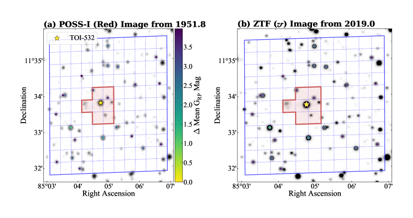
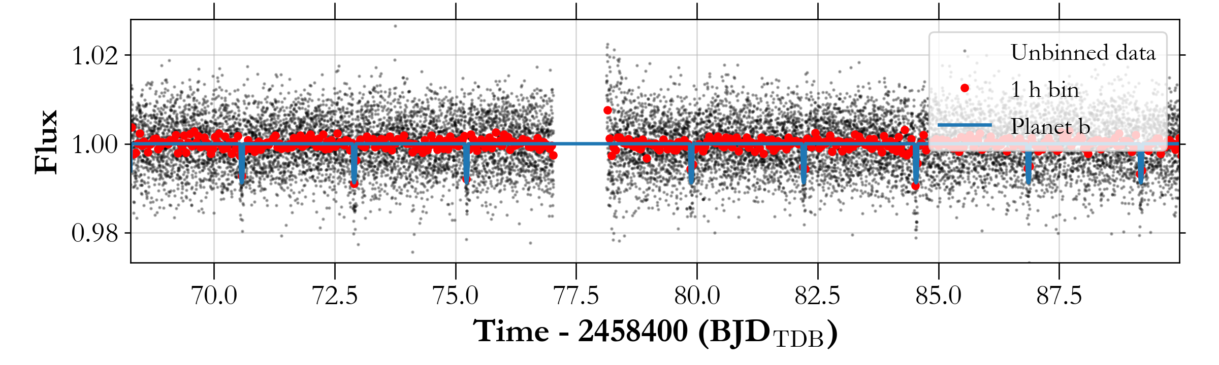
TOI-532 (TIC-144700903, 2MASS J05401918+1133463, Gaia EDR3 3340265717587057536, UCAC4 508-014156) was observed by TESS in Sector 6 in Camera 1 from 2018 December 11 to 2019 January 7th at two minute cadence (Figure 2). The Science Processing Operations Center (SPOC) at NASA Ames (Jenkins et al., 2016) reported one transiting planet candidate, TOI-532.01, with a period of 2.326811 days. For our subsequent analysis, we use the Presearch Data Conditioning Single Aperture Photometry (PDCSAP) lightcurve, which contains systematics and dilution corrected data using the algorithms originally developed for the Kepler data analysis pipeline. We retrieved the data using the lightkurve package (Lightkurve Collaboration et al., 2018), available at the Mikulski Archive for Space Telescopes (MAST).
Figure 1 presents a comparison of the region contained within the Sector 6 footprint from the Palomar Observatory Sky Survey (POSS-1; Harrington, 1952; Minkowski & Abell, 1963) image in 1951 and a more recent ZTF (Masci et al., 2019) image from 2019. There are no bright targets with GRP 3 present in the TESS aperture, however there are a few targets with GRP 4, that dilute the TESS transit. Even though this is taken into account in the PDCSAP flux, following the methodology of Burt et al. (2020) we use our ground based photometry to estimate an additional correction to this dilution term photometry and discuss this in Section 4.
2.2 Ground Based Photometric Follow up
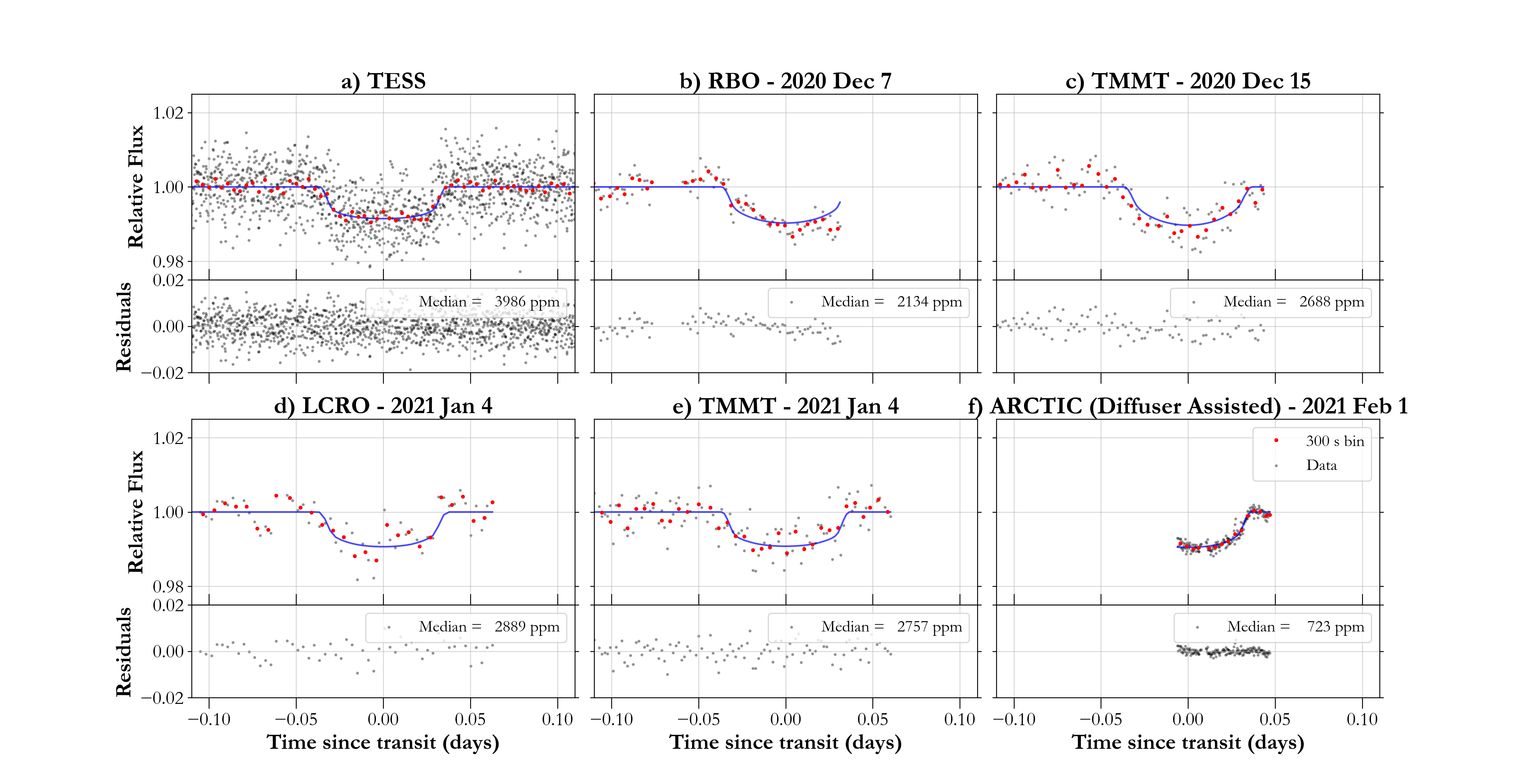
We obtain follow up transits from the ground, to validate the transit seen in the TESS photometry, and measure the dilution present therein. Furthermore, the ground based photometry helps in improving the radius estimates as well as the ephemeris. These observations were pipeline processed using standard linearity, bias, dark, and flat field corrections. We then performed aperture photometry using AstroImageJ (Collins et al., 2017). Clear outliers due to cosmic rays, charged-particle events, poor seeing conditions, or telescope tracking were removed using AstroImageJ. We experimented using a number of different aperture settings, and varied the radii of the photometric aperture, as well as the inner, and outer background annuli, and selected the settings that resulted in the minimum scatter in the resulting photometry. Following the methodology in Stefansson et al. (2017), we added the scintillation error estimates to the photometric error estimated by AstroImageJ. See Figure 3, and Table 1 for a summary of all our ground based photometric observations.
2.2.1 RBO
We observed a transit of TOI-532b on the night of 2020 December 7 using the telescope at the Red Buttes Observatory (RBO) in Wyoming (Kasper et al., 2016). The RBO telescope is a f/8.43 Ritchey-Chrétien Cassegrain constructed by DFM Engineering, Inc. It is currently equipped with an Apogee ASPEN CG47 camera.
The target rose from an airmass of 1.61 at the start of the observations to a minimum airmass of 1.15 and then set to an airmass of 1.20 at the end of the observations. Observations were performed using the Bessell I filter (Bessell, 1990) with on-chip binning. To prevent saturation, we defocused moderately (Table 1), which allowed us to use an exposure time of . In the binning mode, the at RBO has a gain of , a plate scale of , and a readout time of approximately .
Due to cloud contamination, only the transit ingress was recovered from these observations (Figure 3b). For the final reduction, we selected a photometric aperture of 17 pixels (9.04) with an inner sky annulus of 40 pixels (21.3) and outer sky annulus of 60 pixels (31.9).
2.2.2 TMMT
We observed two transits of TOI-532b on the nights of 2020 December 15 (Figure 3c) and 2021 January 4 (Figure 3e) using the Three-hundred MilliMeter () Telescope (TMMT; Monson et al., 2017) at Las Campanas Observatory in Chile. TMMT is a f/7.8 FRC300 from Takahashi on a German equatorial AP1600 GTO mount with an Apogee Alta U42-D09 CCD Camera, FLI ATLAS focuser, and Centerline filter wheel.
On 2020 December 15, the target rose from an airmass of 1.86 at the start of the observations to a minimum airmass of 1.32 and then set to an airmass of 2.62 at the end of the observations. On 2021 January 4, the target rose from an airmass of 1.48 to a minimum airmass of 1.32 and then set to an airmass of 3.16 at the end of observations. Observations on both nights were performed using the Bessell I filter with on-chip binning and exposure times of 120 . In the binning mode, TMMT has a gain of , a plate scale of , and a readout time of .
In addition to the standard corrections, a fringe subtraction was also performed for the TMMT I band images. The final light curve from 2020 December 15 utilized a photometric aperture of 5 pixels (5.97), an inner sky annulus of 20 pixels (23.9), and a outer sky annulus of 30 pixels (35.8). The final light curve from 2021 January 4 utilized a photometric aperture of 5 pixels (5.97), an inner sky annulus of 15 pixels (17.9) and outer sky annulus of 30 pixels (35.8).
2.2.3 LCRO
We observed a transit of TOI-532b on the night of 2021 January 4 (Figure 3d) using the Las Campanas Remote Observatory (LCRO) telescope at the Las Campanas Observatory in Chile. The LCRO telescope is an f/8 Maksutov-Cassegrain from Astro-Physics on a German Equatorial AP1600 GTO mount with an FLI Proline 16803 CCD Camera, FLI ATLAS focuser and Centerline filter wheel.
The target rose from an airmass of 1.40 at the start of the observations to a minimum airmass of 1.32 and then set to an airmass of 3.29 at the end of the observations. Observations were performed using the SDSS filter with on-chip binning and an exposure time of . In the binning mode, LCRO has a gain of , and a plate scale of , and a readout time of . For the final reduction, we selected a photometric aperture of 6 pixels (4.64) with an inner sky annulus of 13 pixels (10.0) and outer sky annulus of 30 pixels (23.2).
2.2.4 Diffuser-assisted Photometry with the 3.5m ARC Telescope
We observed a transit of TOI-532b (Figure 3f) on the night of 2021 February 1 using the Astrophysical Research Consortium (ARC) Telescope Imaging Camera (ARCTIC; Huehnerhoff et al., 2016) at the ARC 3.5m Telescope at Apache Point Observatory (APO). We observed the transit using the Engineered Diffuser available on ARCTIC, which we designed to enable precision photometric observations from the ground on nearby bright stars (Stefansson et al., 2017).
The target set from an airmass of 1.07 at the start of the observations to an airmass of 1.14 at the end of the observations. The observations were performed using the SDSS filter with an exposure time of 20 in the LL-readout and fast readout modes with on-chip binning. In the binning mode, ARCTIC has a gain of , a plate scale of , and a readout time of . Due to cloud contamination, only the egress of the transit was recovered from the data. For the final reduction, we selected a photometric aperture of 13 pixels (5.72), an inner sky annulus of 30 pixels (13.2), and outer sky annulus of 45 pixels (19.8).
| Obs Date | Filter | Exposure | PSF | Apertures: Photometric, | Field of View |
|---|---|---|---|---|---|
| (YYYY-MM-DD) | Time (s) | FWHM (”) | Inner, Outer Annuli (”) | (’) | |
| RBO (0.6 m) | |||||
| 2020-12-07 | Bessell I | 120 | 8.88 (Defocus) | 9.04, 21.3, 31.9 | 8.94 8.94 |
| TMMT (0.3 m) | |||||
| 2020-12-15 | Bessell I | 120 | 3.49 | 5.97, 23.9, 35.8 | 40.75 40.75 |
| 2021-01-04 | Bessell I | 120 | 3.18 | 5.97, 17.9, 35.8 | 40.75 40.75 |
| LCRO (0.3 m) | |||||
| 2021-01-04 | i’ | 240 | 2.45 | 4.64, 10.0, 23.2 | 51.97 51.97 |
| APO (3.5 m) | |||||
| 2021-02-01 | i’ | 20 | 7.67 (Diffusera) | 5.72, 13.2, 19.8 | 7.9 7.9 |
2.3 High Contrast Imaging
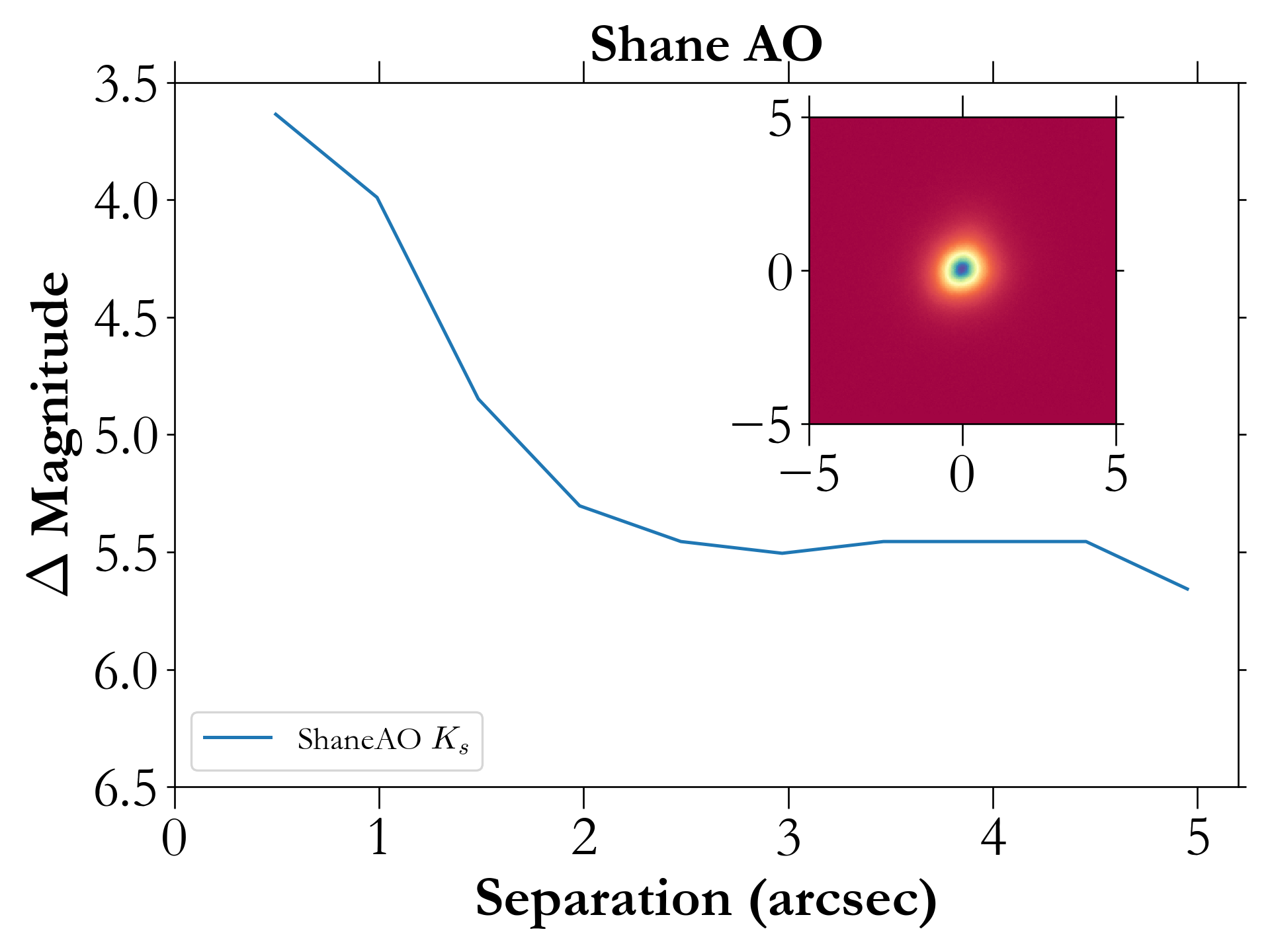
2.3.1 ShARCS on the Shane telescope
We observed TOI-532 using the ShARCS camera on the Shane 3m telescope at Lick Observatory (Srinath et al., 2014). Due to instrument repairs, we were unable to use the Laser Guide Star (LGS) mode, and had to use Natural Guide Star (NGS) mode. This mode can be more challenging for faint targets, as the guider camera can easily lose the target, but conditions were good enough to retrieve data for TOI-532. The target was observed using a 5 point dither process as outlined in Furlan et al. (2017).
The data is then reduced using a custom AO pipeline developed internally. This pipeline first rejects all overexposed or underexposed images, and we then manually exclude data we know to be erroneous (lost guiding on the star, shutters closed early due to weather, etc.). Next we apply a standard dark correction, flat correction, and sigma clipping process. A master sky image is produced from the 5 point dither process, and subtracted from each image. A final image is then produced using an interpolation process to shift the images onto a single centroid.
2.3.2 NESSI at WIYN
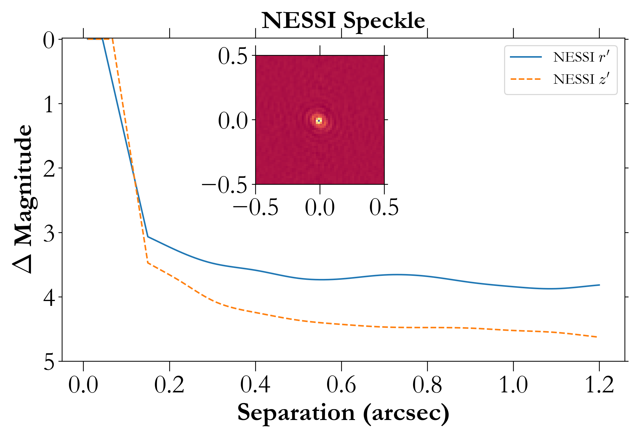
We supplement our AO data with speckle imaging observations taken on 2021 April 3 using the NN-Explore Exoplanet Stellar Speckle Imager (NESSI) on the WIYN 3.5m telescope at Kitt Peak National Observatory. To search for faint background stars and stellar companions, we collected a 9 minute sequence of 40 ms diffraction-limited exposures of TOI-532 with the Sloan and filters. As we show in Figure 4, the NESSI data show no evidence of blending from a bright companion at separations ″at = 3.1, and = 3.5.
2.4 Radial Velocity Follow-up with the Habitable-zone Planet Finder
We observed TOI-532 using HPF (Mahadevan et al., 2012, 2014), a near-infrared ( Å), high resolution precision RV spectrograph located at the 10 meter Hobby-Eberly Telescope (HET) in Texas. HET is a fixed-altitude telescope with a roving pupil design. It is fully queue-scheduled telescope with all observations executed in a queue by the HET resident astronomers (Shetrone et al., 2007). HPF is a fiber-fed instrument with a separate science, sky and simultaneous calibration fiber (Kanodia et al., 2018), and is actively temperature-stabilized at the milli-Kelvin level (Stefansson et al., 2016). We use the algorithms described in the tool HxRGproc for bias removal, non-linearity correction, cosmic ray correction, slope/flux and variance image calculation (Ninan et al., 2018) of the raw HPF data. HPF has the capability for simultaneous calibration using a NIR Laser Frequency Comb (LFC; Metcalf et al., 2019), however owing to the faintness of our target we chose to avoid simultaneous calibration to minimize the impact of scattered calibrator light in the science target spectra. Instead, we interpolate the wavelength solution from other LFC exposures on the night of the observations, to correct for the well calibrated instrument drift, as has been discussed in Stefansson et al. (2020). This method has been shown to enable precise wavelength calibration and drift correction with a precision of cm/s per observation, a value much smaller than our estimated per observation RV uncertainty (instrumental + photon noise) for this object of m/s (in 649 s exposures).
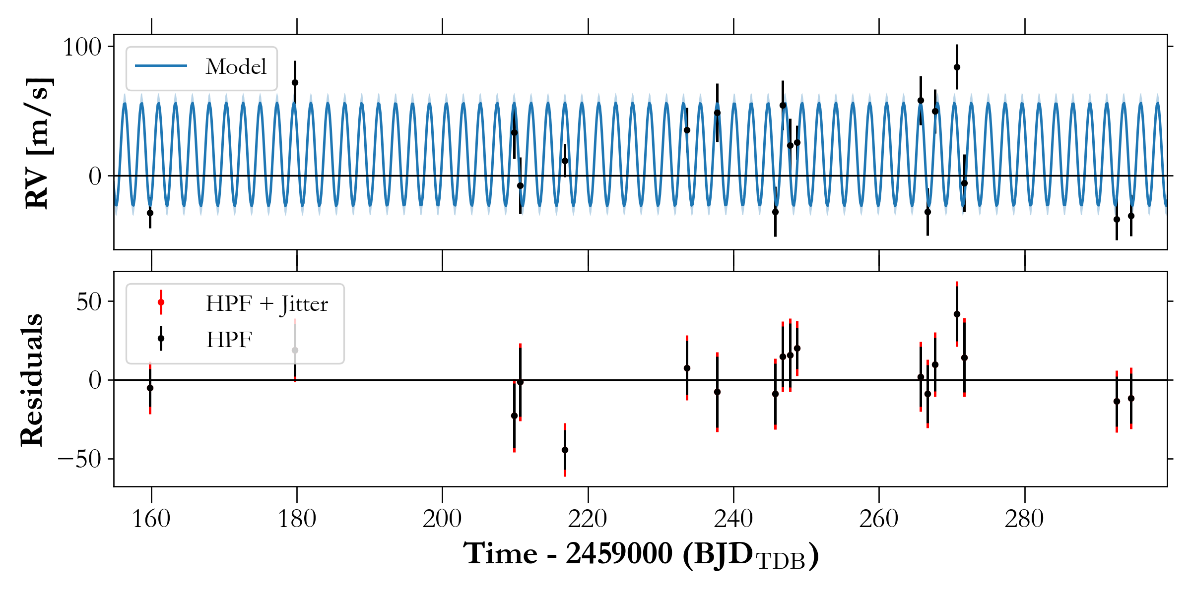
To estimate the RVs, we follow the method described in Stefansson et al. (2020), by using a modified version of the SpEctrum Radial Velocity AnaLyser pipeline (SERVAL; Zechmeister et al., 2018). SERVAL uses the template-matching technique to derive RVs (e.g., Anglada-Escudé & Butler, 2012), where it creates a master template from the target star observations, and determines the Doppler shift for each individual observation by minimizing the statistic. We create this master template by using all the HPF observations of TOI-532, where telluric and sky-emission lines are masked in the calculations of the RVs. The telluric regions identified by a synthetic telluric-line mask generated from telfit (Gullikson et al., 2014), a Python wrapper to the Line-by-Line Radiative Transfer Model package (Clough et al., 2005). Given the faintness of our target, we do not subtract out the sky fiber spectra from the sky fiber, as we observed that doing so added additional read noise, resulting in less precise RV measurements. To perform our barycentric correction, we use barycorrpy, the Python implementation (Kanodia & Wright, 2018) of the algorithms from Wright & Eastman (2014). We obtained a total of 19 visits on this target between 2020 November 5 and 2021 March 21, of which 1 visit was discarded due to bad weather conditions. Each visit was divided into 3 exposures of 649 seconds each, where the median S/N of each HPF exposure was 37 per resolution element. The individual exposures were then binned after weighting, with the final binned RVs being listed in Table 2 and plotted in Figure 6.
| RV | ||
|---|---|---|
| (d) | ||
| 2459159.82217 | -28.41 | 12.02 |
| 2459179.76468 | 72.25 | 16.71 |
| 2459209.85498 | 33.54 | 20.41 |
| 2459210.67441 | -7.51 | 21.93 |
| 2459216.82807 | 11.79 | 12.70 |
| 2459233.61084 | 35.41 | 17.17 |
| 2459237.77469 | 48.57 | 22.57 |
| 2459245.75139 | -27.58 | 19.35 |
| 2459246.74596 | 54.53 | 19.16 |
| 2459247.75757 | 23.59 | 20.39 |
| 2459248.74084 | 25.75 | 13.16 |
| 2459265.69221 | 58.13 | 19.00 |
| 2459266.69484 | -27.78 | 18.47 |
| 2459267.68911 | 49.75 | 16.90 |
| 2459270.68444 | 84.04 | 17.46 |
| 2459271.68015 | -5.66 | 22.22 |
| 2459292.62161 | -33.47 | 15.94 |
| 2459294.61636 | -30.69 | 15.83 |
3 Stellar Parameters
| Parameter | Description | Value | Reference |
|---|---|---|---|
| Main identifiers: | |||
| TOI | TESS Object of Interest | 532 | TESS mission |
| TIC | TESS Input Catalogue | 144700903 | Stassun |
| 2MASS | J05401918+1133463 | 2MASS | |
| WISE | J054019.20+113345.6 | WISE | |
| Gaia EDR3 | 3340265717587057536 | Gaia EDR3 | |
| Equatorial Coordinates, Proper Motion and Spectral Type: | |||
| Right Ascension (RA, degrees) | 85.08005702(4) | Gaia EDR3 | |
| Declination (Dec, degrees) | 11.562632056(3) | Gaia EDR3 | |
| Proper motion (RA, ) | Gaia EDR3 | ||
| Proper motion (Dec, ) | Gaia EDR3 | ||
| Distance in pc | Bailer-Jones | ||
| Maximum visual extinction | 0.01 | Green | |
| Optical and near-infrared magnitudes: | |||
| Johnson B mag | APASS | ||
| Johnson V mag | APASS | ||
| Sloan mag | APASS | ||
| Sloan mag | APASS | ||
| Sloan mag | APASS | ||
| TESS magnitude | Stassun | ||
| mag | 2MASS | ||
| mag | 2MASS | ||
| mag | 2MASS | ||
| WISE1 mag | WISE | ||
| WISE2 mag | WISE | ||
| WISE3 mag | WISE | ||
| Spectroscopic Parametersa: | |||
| Effective temperature in | This work | ||
| Metallicity in dex | This work | ||
| Surface gravity in cgs units | This work | ||
| Model-Dependent Stellar SED and Isochrone fit Parametersb: | |||
| Effective temperature in | This work | ||
| Metallicity in dex | This work | ||
| Surface gravity in cgs units | This work | ||
| Mass in | This work | ||
| Radius in | This work | ||
| Luminosity in | This work | ||
| Density in | This work | ||
| Age | Age in Gyrs | This work | |
| Other Stellar Parameters: | |||
| Rotational velocity in | km/s | This work | |
| “Absolute” radial velocity in | This work | ||
| Galactic velocities (Barycentric) in | This work | ||
| Galactic velocities (LSR) in | This work | ||
3.1 Spectroscopic Parameters with HPF-SpecMatch
Using the method described in Stefansson et al. (2020), we use the HPF spectra to estimate the , , and [Fe/H] values of the host star. This is based on SpecMatch-Emp algorithm from Yee et al. (2017), where we compare the high resolution HPF spectra of TOI-532 to a library of high S/N as-observed HPF spectra, which consists of slowly-rotating reference stars with well characterized stellar parameters from Yee et al. (2017).
We shift the observed target spectrum to a library wavelength scale and rank all of the targets in the library using a goodness-of-fit metric. After this initial minimization step, we pick the five best matching reference spectra (in this case: BD+29 2279, GJ 134, GJ 205, HD 28343, HD 88230) to construct a weighted spectrum using their linear combination to better match to the target spectrum (Jones et al. 2021 in prep.). In this step, each of the five stars receives a best-fit weight coefficient. We then assign the target stellar parameter , , and [Fe/H] values as the weighted average of the five best stars using the best-fit weight coefficients. Our final parameters are listed in Table 3, and are derived from the HPF order spanning 8670 – 8750 Å. As an additional check, we performed a similar library comparison using 6 other HPF orders which have low telluric contamination, and obtain consistent stellar parameters across them. Our error estimates are obtained from using the cross-validation method, as described by Stefansson et al. (2020). During both optimization steps, we account for any potential broadening by artificially broadening the library spectra with a broadening kernel (Gray, 1992) to match the rotational broadening of the target star. For TOI-532, we did not need significant rotational broadening, and therefore place an upper limit of , which is the lower limit of measurable values given HPF’s spectral resolving power of .
3.2 Model-Dependent Stellar Parameters
In addition to the spectroscopic stellar parameters derived above, we use EXOFASTv2 (Eastman et al., 2013) to model the SED of TOI-532 to derive model-dependent constraints on the stellar mass, radius, and age of the star. For the spectral energy distribution (SED) fit, EXOFASTV2 uses the BT-NextGen stellar atmospheric models (Allard et al., 2012). We assume Gaussian priors on the (i) 2MASS magnitudes, (ii) SDSS and Johnson and magnitudes from APASS, (iii) Wide-field Infrared Survey Explorer magnitudes , , and , (Wright et al., 2010), (iv) spectroscopically-derived host star effective temperature, surface gravity, and metallicity, and (v) distance estimate from Bailer-Jones et al. (2021). We apply a uniform prior on the visual extinction and place an upper limit using estimates of Galactic dust by Green et al. (2019) (Bayestar19) calculated at the distance determined by Bailer-Jones et al. (2021). We convert the Bayestar19 upper limit to a visual magnitude extinction using the reddening law from Fitzpatrick (1999).
We use GALPY (Bovy, 2015) to calculate the UVW velocities in the barycentric frame222With U towards the Galactic center, V towards the direction of Galactic spin, and W towards the North Galactic Pole (Johnson & Soderblom, 1987)., which along with the BANYAN tool (Gagné et al., 2018) classify TOI-532 as a field star in the thin disk with very high probability (Bensby et al., 2014).
3.3 Estimating Rotation Period
We note that the TESS photometry (PDCSAP undetrended photometry shown in Figure 2) is relatively flat, and shows no flaring activity. We also run a generalized Lomb Scargle (GLS) periodogram (Zechmeister & Kürster, 2009) on the TESS photometry using its astropy implementation, and find no significant peaks with a False Alarm Probability 333The PDCSAP photometry from TESS flattens variability on timescales longer than about 10 days (Jenkins et al., 2016), and therefore our search using the TESS photometry is insensitive to stellar rotation periods longer than this.. This is consistent with an inactive star with a long rotation period.
4 Joint Fitting of Photometry and RVs
We perform a joint fit of all the photometry (TESS + ground based sources), and the RVs using the Python packge exoplanet, which uses PyMC3 the Hamiltonian Monte Carlo (HMC) package (Salvatier et al., 2016).
The exoplanet package uses starry (Luger et al., 2019; Agol et al., 2020) to model the planetary transits, using the analytical transit models from Mandel & Agol (2002), which includes a quadratic limb darkening law. These limb darkening priors are implemented in exoplanet using the reparameterization suggested by Kipping (2013) for uninformative sampling. We fit each phased transit shown in Figure 3 with separate limb darkening coefficients444We also try fitting the photometry with a single set of limb darkening coefficients for all the transits, and obtain similar results.. In the photometric model we include a dilution factor for the TESS photometry, , to represent the ratio of the out-of-transit flux of TOI-532 to that of all the stars within the TESS aperture, that has not been corrected for. We assume that the higher spatial resolution ground based photometry has no dilution, since we use the ground based transits to estimate the dilution in the TESS photometry. We assume the transit depth is identical in all bandpasses and use our ground-based transits to determine the dilution required in the TESS data to be ; including which, gives us a radius of . If the blending effects due to background stars are correctly accounted for by the SPOC pipeline, we expect this dilution term to be close to 1.
We model the RVs using a standard Keplerian model. We try an eccentric joint fit to the photometry and RVs, and obtain an eccentricity consistent with a circular orbit at . Considering the Lucy-Sweeney bias (Lucy & Sweeney, 1971), we adopt a circular orbit by fixing the eccentricity to 0, and the argument of periastron to 90∘. For both the photometry and RV modeling, we include a simple white-noise model in the form of a jitter term that is added in quadrature to the error bars of each data set.
We use scipy.optimize to find the initial maximum a posteriori (MAP) parameter estimates, which are then used as the initial conditions for parameter estimation using ”No U-Turn Sampling” (NUTS, Hoffman & Gelman, 2014), implemented for the HMC sampler PyMC3, where we check for convergence using the Gelman-Rubin statistic (; Ford, 2006). We also run a joint fit using juliet (Espinoza et al., 2019), and verify that we obtain fit parameters similar to those from exoplanet.
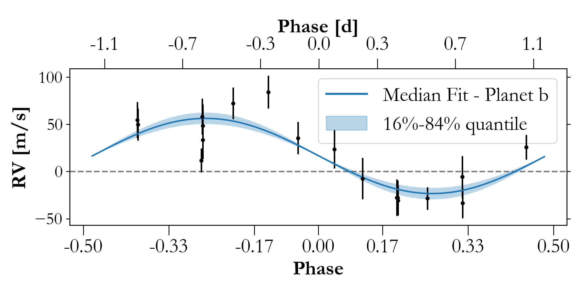
The host stellar density constrained from the transit fit to the TESS photometry (Seager & Mallén-Ornelas, 2003) is consistent with that obtained from the SED fit for an M0 host star (Section 3.2). The final derived planet parameters are shown in Table 4, and the phased HPF RVs are shown in Figure 7. We obtain a mass for TOI-532b of M⊕, and a radius of R⊕.
| Parameter | Units | Value |
|---|---|---|
| Orbital Parameters: | ||
| Orbital Period | (days) | 2.3266508 |
| Eccentricity | 0 (fixed) | |
| Argument of Periastron | (degrees) | 90 (fixed) |
| Semi-amplitude Velocity | (m/s) | 39.82 |
| Systemic Velocitya | (m/s) | 16.42 |
| RV trend | () | 0.35 |
| RV jitter | (m/s) | 11.43 |
| Transit Parameters: | ||
| Transit Midpoint | (BJDTDB) | 2458470.576777 |
| Scaled Radius | ||
| Scaled Semi-major Axis | 10.49 | |
| Orbital Inclination | (degrees) | 88.08 |
| Transit Duration | (days) | 0.07280.001 |
| Photometric Jitterb | (ppm) | |
| (ppm) | ||
| (ppm) | ||
| (ppm) | ||
| (ppm) | ||
| (ppm) | ||
| Dilutionc | ||
| Planetary Parameters: | ||
| Mass | (M⊕) | |
| Radius | (R⊕) | |
| Density | (g/) | |
| Semi-major Axis | (AU) | |
| Average Incident Fluxd | () | 1.280.11 |
| Planetary Insolation | (S⊕) | |
| Equilibrium Temperaturee | (K) | |
5 Discussion
5.1 Giant Planet Dependence on Host Star Metallicity
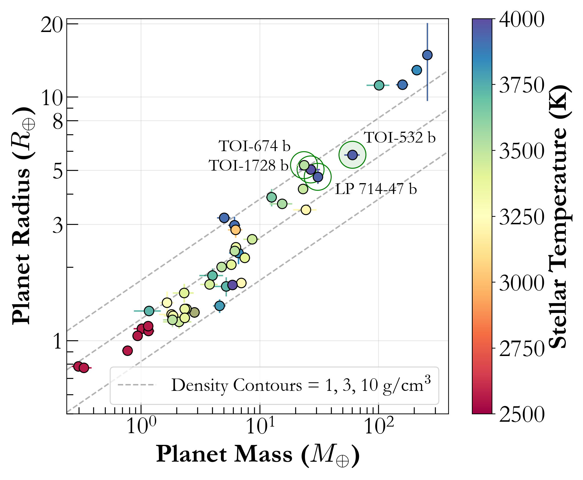
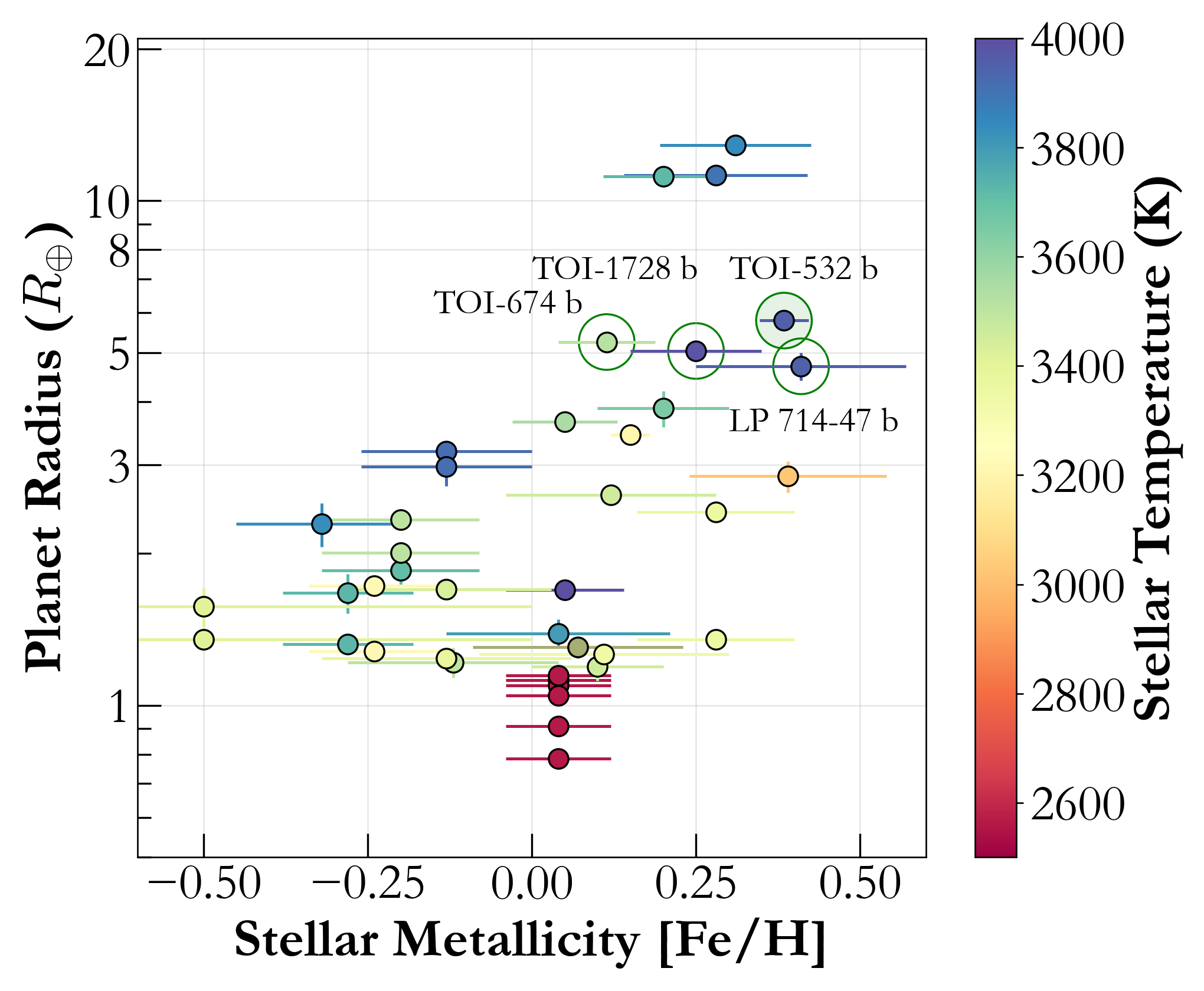
In Figure 10a we show TOI-532 b with respect to other M dwarf exoplanets with mass measurements at 3 or higher. The data is taken from the NASA Exoplanet Archive (Akeson et al., 2013), and includes recent M dwarf transiting planets discovered by TESS. TOI-532b has properties similar to three recent super Neptunes discovered by TESS that orbit M dwarf stars - TOI-1728b (Kanodia et al., 2020), LP 714-417b (TOI-442 b; Dreizler et al., 2020), and TOI-674b (Murgas et al., 2021). TOI-532b represents the largest and most massive Super Neptune found orbiting an M dwarf.
TOI-532b orbits a metal-rich M star, similar to the other gas giants found around M dwarfs (Figure 10b). This positive metallicity correlation favours the core-accretion formation mechanism (Pollack et al., 1996; Schlaufman, 2018); which can be explained if these gas giants formed due to the collisions of 10 cores . The probability of formation of these cores increases with metallicity, and therefore it should be easier to form such gaseous planet cores around metal-rich stars, before the protoplanetary disk depletes (Ida & Lin, 2004b). In-situ formation of these gas giants at such orbital periods (and hence orbital separations) also requires super-Solar metallicity protoplanetary disks to provide enough material for the formation of their cores (Dawson et al., 2015; Boley et al., 2016; Batygin et al., 2016).
An alternative to the accretion theories of formation , is gravitational instability (GI; Boss, 1997). This has been proposed to explain the formation of gas giants around these low mass stars (Boss, 2006), especially the mid-to-late M dwarfs (Morales et al., 2019). The amount of material available in these disks would be too little to form cores that are massive enough to accrete gaseous envelopes from the disk before it gets depleted (Laughlin et al., 2004), lending credibility to GI as a potential formation mechanism. The discovery of gas giants such as TOI-532b, adds to the sparse population of these objects around M dwarfs, which can ultimately help differentiate between these two competing theories.
5.2 Neptune desert
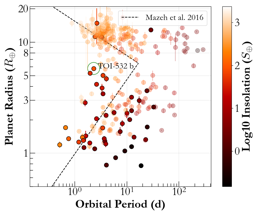
Figure 13 shows the Neptune desert which is characterized by a dearth of planets. We highlight the location of TOI-532b in the Neptune desert (Mazeh et al., 2016) in the Radius–Period plane (Figure 13a), where it falls in the middle of this region. The figure includes transiting exoplanets with mass measurements, coloured according to their insolation, with the M dwarf planets shown as solid markers, whereas those orbiting other spectral types hosts are translucent. Different processes have been proposed to explain this feature, which include photoevaporation (Owen & Lai, 2018; Ionov et al., 2018), and high eccentricity migration (Matsakos & Königl, 2016).
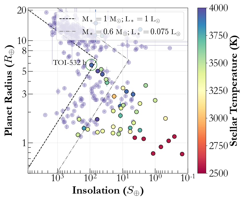
Although typically parameterized in terms of orbital period, it is important to consider that in a combined sample of FGK and M dwarf host stars, the bolometric insolation can differ by more than an order of magnitude for similar orbital separations (e.g., between a G type host, and an early M dwarf). McDonald et al. (2019) suggest that this variation in the bolometric luminosity is the primary reason for the discrepancies in the location of the Neptune desert as a function of spectral type. Therefore, we also plot TOI-532 in the Radius–Insolation plane (Figure 13b), and include the desert boundaries from Mazeh et al. (2016) which were estimated using a predominantly FGK planet sample. We include these in the Insolation–Radius plane assuming a Solar mass and luminosity, and also assuming an M0 host star. While TOI-532 is located inside the Neptune desert in the Radius–Period plane, when accounting for the incident insolation, it is located by the edge of this desert. We therefore suggest that in order to compare a sample of planets across spectral types FGK, and M, the Neptune desert should be characterized in the Radius–Insolation plane.
The under-density of planets in this highly irradiated region has often been attributed to atmospheric escape due to photoevaporation (Owen & Lai, 2018). The rate and efficacy of photoevaporation is highly dependent on the X-ray and ultraviolet flux (XUV) from the host star; where a planet around a mid-type M dwarf can receive 100x more integrated X-ray flux than a solar type star (for the same insolation). When the frequency distribution of these gaseous planets is considered as a function of lifetime integrated X-ray flux, most of the variability between spectral types is accounted for (McDonald et al., 2019).
Characterization of planets such as TOI-532b, which lie within the Neptune desert, can help provide constraints on the potential formation mechanisms responsible for clearing out the Neptune desert. Estimating the fraction of H/He within its atmosphere would help bound the extent of photoevaporation, and its role in sculpting this desert. TOI-532b helps increase the small sample of planets situated inside this desert. Comparing the stellar (metallicity, age, stellar mass) and planetary parameters (density, planetary mass) for the sample of planets inside the desert to the larger exoplanet sample can help highlight potential formation mechanisms; perhaps as an extension to the radius valley (Fulton et al., 2017), and it’s dependence on various stellar properties (Owen & Murray-Clay, 2018; Cloutier et al., 2019; Berger et al., 2020; Van Eylen et al., 2021).
5.3 Planetary Composition and Photoevaporation
We use the giant planet models from Fortney et al. (2007) to estimate a core mass of M⊕ for TOI-532b, corresponding to an atmospheric mass (H/He) fraction of . Super Neptunes such as TOI-532b present an intermediate population of gaseous planets between sub-Neptunes (Bean et al., 2021) and Jovian planets (Mordasini et al., 2016; Dawson & Johnson, 2018). A subset of these Super Neptunes with equilibrium temperatures between 800–1200 K span the range where models predict a transition from methane dominated atmospheres to carbon monoxide (Guzmán-Mesa et al., 2020). Characterizing the atmospheres of planets such as TOI-532b with equilibrium temperatures of K by constraining their C/H and C/O ratios, can help place constraints on their formation history as well as atmospheric chemistry (Madhusudhan et al., 2017).
TOI-532 is relatively faint (J = 11.46), but is still accessible from 10-m class telescopes (Tamura et al., 2012; Kotani et al., 2018), as a potential target for detecting atmospheric escape using the He 10830 Å triplet. Considering the small number of suitable targets for such a measurement, we discuss the possibility of detecting atmospheric escape from TOI-532b. It is useful to compare TOI-532b to a similar planet with such a detection—GJ 3470b (Ninan et al., 2020; Palle et al., 2020)—and also to a planet without a He 10830 Å detection, TOI-1728b (Kanodia et al., 2020). In the energy limited mass outflow regime555The energy limited regime is a reasonable assumption here since the gravitational potential of this planet is 12.81 erg g-1 (log10 (GM/R); Salz et al., 2016) . This is not a system with a low density upper-atmosphere, like those seen in planets with higher gravitational potential (13.3 erg g-1), the exosphere outflow is proportional to the irradiated extreme ultra violet (EUV) flux and inversely proportional to the planet density. TOI-532 is an earlier M0 star than the M1.5 GJ 3470, with its spectral type more favourable with higher EUV radiation. However, TOI-532 is an older (and quieter) Gyr star, while GJ 3470 is relatively young at Gyr666GJ 3470b stellar and planetary parameters are from Kosiarek et al. (2019).. If we consider the EUV flux from the host star to be similar, due to the larger radius of the host star, the EUV irradiance on TOI-532b is 1.6 times that of GJ 3470b, which can make up for the 1.8 times higher density of TOI-532b than GJ 3470b. Thus, if the EUV flux of TOI-532 (7 Gyr, M0) is similar to GJ 3470 (3 Gyr, M1.5), we could expect a similar exosphere evaporation and mass outflow in TOI-532b like in GJ 3470b. Under this condition, He 10830 Å absorption during transit is a good probe to detect any signatures of outflow from TOI-532.
Conversely, the other planet TOI-1728b has a host star very similar to TOI-532 in both spectral type and age. TOI-532 orbits 1.25 times closer than TOI-1728b, and it is 1.5 times denser than TOI-1728b. Therefore, from a simple scaling relationship we expect the mass outflows in them to be only slightly less or very similar. That being said, TOI-1728b had a null detection of He 10830 Å with an upper limit of 1.1% (Kanodia et al., 2020). We therefore note that though the planetary parameters are amenable, the plausibility of a detectable outflow from this super Neptune hinges on the EUV irradiation environment of the host star.
6 Summary
In this work, we report the discovery and confirmation of a super Neptune, TOI-532b, orbiting an M0 star in a 2.3 day circular orbit. We detail the TESS photometry, ground-based follow-up photometry, high contrast imaging, and also the RV observations performed using HPF. Furthermore, we discuss how the planet is situated at the edge of the Neptune desert in the Radius–Insolation plane, and discuss potential for He 10830 Å absorption detection using transmission spectroscopy. We also discuss the metallicity correlation for gas giants occurrence, and how it continues down to the M dwarf spectral type.
The discovery and mass measurement of gas giants such as TOI-532b adds to the small sample of such planets around M dwarf host stars, and can help inform theories of planetary formation and evolution. Therefore we encourage future observations to place limits on atmospheric escape using the He 10830 Å transition.
7 Acknowledgements
This research made use of Lightkurve, a Python package for Kepler and TESS data analysis (Lightkurve Collaboration, 2018).
This paper is based on observations obtained from the Las Campanas Remote Observatory that is a partnership between Carnegie Observatories, The Astro-Physics Corporation, Howard Hedlund, Michael Long, Dave Jurasevich, and SSC Observatories.
This work has made use of data from the European Space Agency (ESA) mission Gaia (https://www.cosmos.esa.int/gaia), processed by the Gaia Data Processing and Analysis Consortium (DPAC, https://www.cosmos.esa.int/web/gaia/dpac/consortium). Funding for the DPAC has been provided by national institutions, in particular the institutions participating in the Gaia Multilateral Agreement.
The Center for Exoplanets and Habitable Worlds is supported by the Pennsylvania State University, the Eberly College of Science, and the Pennsylvania Space Grant Consortium. These results are based on observations obtained with the Habitable-zone Planet Finder Spectrograph on the HET. We acknowledge support from NSF grants AST 1006676, AST 1126413, AST 1310875, AST 1310885, and the NASA Astrobiology Institute (NNA09DA76A) in our pursuit of precision radial velocities in the NIR. We acknowledge support from the Heising-Simons Foundation via grant 2017-0494. The Hobby-Eberly Telescope is a joint project of the University of Texas at Austin, the Pennsylvania State University, Ludwig-Maximilians-Universität München, and Georg-August Universität Gottingen. The HET is named in honor of its principal benefactors, William P. Hobby and Robert E. Eberly. The HET collaboration acknowledges the support and resources from the Texas Advanced Computing Center. We thank the Resident astronomers and Telescope Operators at the HET for the skillful execution of our observations with HPF.
We acknowledge support from NSF grants AST-1909506 and AST-1907622 and the Research Corporation for precision photometric observations with diffuser-assisted photometry.
This work was performed under the following financial assistance award 70NANB18H006 from U.S. Department of Commerce, National Institute of Standards and Technology
This research has made use of the NASA Exoplanet Archive, which is operated by the California Institute of Technology, under contract with the National Aeronautics and Space Administration under the Exoplanet Exploration Program. This work includes data collected by the TESS mission, which are publicly available from MAST. Funding for the TESS mission is provided by the NASA Science Mission directorate. Some of the data presented in this paper were obtained from MAST. Support for MAST for non-HST data is provided by the NASA Office of Space Science via grant NNX09AF08G and by other grants and contracts.
This research has made use of the SIMBAD database, operated at CDS, Strasbourg, France, and NASA’s Astrophysics Data System Bibliographic Services.
Some of the observations in this paper made use of the NN-EXPLORE Exoplanet and Stellar Speckle Imager (NESSI). NESSI was funded by the NASA Exoplanet Exploration Program and the NASA Ames Research Center. NESSI was built at the Ames Research Center by Steve B. Howell, Nic Scott, Elliott P. Horch, and Emmett Quigley.
Part of this research was carried out at the Jet Propulsion Laboratory, California Institute of Technology, under a contract with the National Aeronautics and Space Administration (NASA).
Computations for this research were performed on the Pennsylvania State University’s Institute for Computational and Data Sciences Advanced CyberInfrastructure (ICDS-ACI), including the CyberLAMP cluster supported by NSF grant MRI-1626251. This work includes data from 2MASS, which is a joint project of the University of Massachusetts and IPAC at Caltech funded by NASA and the NSF. CIC acknowledges support by NASA Headquarters under the NASA Earth and Space Science Fellowship Program through grant 80NSSC18K1114. SK would like to acknowledge Monae and Theodora for help with this project.
This research made use of exoplanet (Foreman-Mackey et al., 2021a) and its dependencies (Agol et al., 2020; Kumar et al., 2019; Robitaille et al., 2013; Astropy Collaboration et al., 2018; Kipping, 2013; Luger et al., 2019; The Theano Development Team et al., 2016; Salvatier et al., 2016; Foreman-Mackey et al., 2021b)
References
- Agol et al. (2020) Agol, E., Luger, R., & Foreman-Mackey, D. 2020, The Astronomical Journal, 159, 123. https://ui.adsabs.harvard.edu/abs/2020AJ....159..123A
- Akeson et al. (2013) Akeson, R. L., Chen, X., Ciardi, D., et al. 2013, Publications of the Astronomical Society of the Pacific, 125, 989. http://adsabs.harvard.edu/abs/2013PASP..125..989A
- Allard et al. (2012) Allard, F., Homeier, D., & Freytag, B. 2012, Philosophical Transactions of the Royal Society of London Series A, 370, 2765. http://adsabs.harvard.edu/abs/2012RSPTA.370.2765A
- Anglada-Escudé & Butler (2012) Anglada-Escudé, G., & Butler, R. P. 2012, The Astrophysical Journal Supplement Series, 200, 15. https://doi.org/10.1088%2F0067-0049%2F200%2F2%2F15
- Astropy Collaboration et al. (2018) Astropy Collaboration, Price-Whelan, A. M., Sipőcz, B. M., et al. 2018, The Astronomical Journal, 156, 123. https://ui.adsabs.harvard.edu/abs/2018AJ....156..123A
- Bailer-Jones et al. (2021) Bailer-Jones, C. A. L., Rybizki, J., Fouesneau, M., Demleitner, M., & Andrae, R. 2021, The Astronomical Journal, 161, 147. http://adsabs.harvard.edu/abs/2021AJ....161..147B
- Bailer-Jones et al. (2018) Bailer-Jones, C. A. L., Rybizki, J., Fouesneau, M., Mantelet, G., & Andrae, R. 2018, The Astronomical Journal, 156, 58. http://adsabs.harvard.edu/abs/2018AJ....156...58B
- Bakos et al. (2015) Bakos, G. A., Penev, K., Bayliss, D., et al. 2015, The Astrophysical Journal, 813, 111. http://adsabs.harvard.edu/abs/2015ApJ...813..111B
- Batygin et al. (2016) Batygin, K., Bodenheimer, P. H., & Laughlin, G. P. 2016, The Astrophysical Journal, 829, 114. https://ui.adsabs.harvard.edu/abs/2016ApJ...829..114B
- Bean et al. (2021) Bean, J. L., Raymond, S. N., & Owen, J. E. 2021, Journal of Geophysical Research (Planets), 126, e06639. https://ui.adsabs.harvard.edu/abs/2021JGRE..12606639B
- Bensby et al. (2014) Bensby, T., Feltzing, S., & Oey, M. S. 2014, Astronomy and Astrophysics, 562, A71. http://adsabs.harvard.edu/abs/2014A%26A...562A..71B
- Berger et al. (2020) Berger, T. A., Huber, D., Gaidos, E., van Saders, J. L., & Weiss, L. M. 2020, The Astronomical Journal, 160, 108. https://ui.adsabs.harvard.edu/abs/2020AJ....160..108B
- Bessell (1990) Bessell, M. S. 1990, Publications of the Astronomical Society of the Pacific, 102, 1181. https://ui.adsabs.harvard.edu/abs/1990PASP..102.1181B/abstract
- Boley et al. (2016) Boley, A. C., Granados Contreras, A. P., & Gladman, B. 2016, The Astrophysical Journal, 817, L17. https://ui.adsabs.harvard.edu/abs/2016ApJ...817L..17B
- Boss (1997) Boss, A. P. 1997, Science, 276, 1836, num Pages: 4 Place: Washington, United States Publisher: The American Association for the Advancement of Science. http://search.proquest.com/docview/213571305/abstract/1B11458F49AA44FBPQ/1
- Boss (2006) —. 2006, The Astrophysical Journal, 643, 501. http://adsabs.harvard.edu/abs/2006ApJ...643..501B
- Bovy (2015) Bovy, J. 2015, The Astrophysical Journal Supplement Series, 216, 29. http://adsabs.harvard.edu/abs/2015ApJS..216...29B
- Burt et al. (2020) Burt, J. A., Nielsen, L. D., Quinn, S. N., et al. 2020, The Astronomical Journal, 160, 153. https://ui.adsabs.harvard.edu/abs/2020AJ....160..153B
- Cañas et al. (2020) Cañas, C. I., Stefansson, G., Kanodia, S., et al. 2020, The Astronomical Journal, 160, 147. http://adsabs.harvard.edu/abs/2020AJ....160..147C
- Clough et al. (2005) Clough, S. A., Shephard, M. W., Mlawer, E. J., et al. 2005, Journal of Quantitative Spectroscopy and Radiative Transfer, 91, 233. http://adsabs.harvard.edu/abs/2005JQSRT..91..233C
- Cloutier et al. (2019) Cloutier, R., Astudillo-Defru, N., Bonfils, X., et al. 2019, Astronomy and Astrophysics, 629, A111. https://ui.adsabs.harvard.edu/abs/2019A&A...629A.111C
- Collins et al. (2017) Collins, K. A., Kielkopf, J. F., Stassun, K. G., & Hessman, F. V. 2017, The Astronomical Journal, 153, 77. http://adsabs.harvard.edu/abs/2017AJ....153...77C
- Cutri et al. (2003) Cutri, R. M., Skrutskie, M. F., van Dyk, S., et al. 2003, ”The IRSA 2MASS All-Sky Point Source Catalog, NASA/IPAC Infrared Science Archive. http://irsa.ipac.caltech.edu/applications/Gator/”. http://adsabs.harvard.edu/abs/2003tmc..book.....C
- Dawson et al. (2015) Dawson, R. I., Chiang, E., & Lee, E. J. 2015, Monthly Notices of the Royal Astronomical Society, 453, 1471. http://adsabs.harvard.edu/abs/2015MNRAS.453.1471D
- Dawson & Johnson (2018) Dawson, R. I., & Johnson, J. A. 2018, Annual Review of Astronomy and Astrophysics, 56, 175. http://adsabs.harvard.edu/abs/2018ARA%26A..56..175D
- Dreizler et al. (2020) Dreizler, S., Crossfield, I. J. M., Kossakowski, D., et al. 2020, Astronomy and Astrophysics, 644, A127. https://ui.adsabs.harvard.edu/abs/2020A&A...644A.127D/abstract
- Dressing & Charbonneau (2015) Dressing, C. D., & Charbonneau, D. 2015, The Astrophysical Journal, 807, 45. http://adsabs.harvard.edu/abs/2015ApJ...807...45D
- Eastman et al. (2013) Eastman, J., Gaudi, B. S., & Agol, E. 2013, Publications of the Astronomical Society of the Pacific, 125, 83. https://iopscience.iop.org/article/10.1086/669497/meta
- Espinoza et al. (2019) Espinoza, N., Kossakowski, D., & Brahm, R. 2019, Monthly Notices of the Royal Astronomical Society, 490, 2262. http://adsabs.harvard.edu/abs/2019MNRAS.490.2262E
- Espinoza et al. (2016) Espinoza, N., Bayliss, D., Hartman, J. D., et al. 2016, The Astronomical Journal, 152, 108. http://adsabs.harvard.edu/abs/2016AJ....152..108E
- Fitzpatrick (1999) Fitzpatrick, E. L. 1999, Publications of the Astronomical Society of the Pacific, 111, 63. http://adsabs.harvard.edu/abs/1999PASP..111...63F
- Ford (2006) Ford, E. B. 2006, The Astrophysical Journal, 642, 505. http://adsabs.harvard.edu/abs/2006ApJ...642..505F
- Foreman-Mackey et al. (2021a) Foreman-Mackey, D., Savel, A., Luger, R., et al. 2021a, exoplanet-dev/exoplanet v0.4.4, doi:10.5281/zenodo.1998447. https://doi.org/10.5281/zenodo.1998447
- Foreman-Mackey et al. (2021b) Foreman-Mackey, D., Luger, R., Agol, E., et al. 2021b, arXiv:2105.01994 [astro-ph], arXiv: 2105.01994. http://arxiv.org/abs/2105.01994
- Fortney et al. (2021) Fortney, J. J., Dawson, R. I., & Komacek, T. D. 2021, Journal of Geophysical Research (Planets), 126, e06629. https://ui.adsabs.harvard.edu/abs/2021JGRE..12606629F
- Fortney et al. (2007) Fortney, J. J., Marley, M. S., & Barnes, J. W. 2007, ApJ, 659, 1661. https://ui.adsabs.harvard.edu/abs/2007ApJ...659.1661F/abstract
- Fulton et al. (2017) Fulton, B. J., Petigura, E. A., Howard, A. W., et al. 2017, The Astronomical Journal, 154, 109. https://ui.adsabs.harvard.edu/abs/2017AJ....154..109F/abstract
- Furlan et al. (2017) Furlan, E., Ciardi, D. R., Everett, M. E., et al. 2017, The Astronomical Journal, 153, 71. http://adsabs.harvard.edu/abs/2017AJ....153...71F
- Gagné et al. (2018) Gagné, J., Mamajek, E. E., Malo, L., et al. 2018, The Astrophysical Journal, 856, 23. http://adsabs.harvard.edu/abs/2018ApJ...856...23G
- Gaia Collaboration et al. (2020) Gaia Collaboration, Brown, A. G. A., Vallenari, A., et al. 2020, arXiv e-prints, 2012, arXiv:2012.01533. http://adsabs.harvard.edu/abs/2020arXiv201201533G
- Gaidos et al. (2013) Gaidos, E., Fischer, D. A., Mann, A. W., & Howard, A. W. 2013, The Astrophysical Journal, 771, 18. http://adsabs.harvard.edu/abs/2013ApJ...771...18G
- Ginsburg et al. (2019) Ginsburg, A., Sipőcz, B. M., Brasseur, C. E., et al. 2019, The Astronomical Journal, 157, 98. http://adsabs.harvard.edu/abs/2019AJ....157...98G
- Gray (1992) Gray, D. F. 1992, Camb. Astrophys. Ser., Vol. 20,. http://adsabs.harvard.edu/abs/1992oasp.book.....G
- Green et al. (2019) Green, G. M., Schlafly, E., Zucker, C., Speagle, J. S., & Finkbeiner, D. 2019, The Astrophysical Journal, 887, 93. http://adsabs.harvard.edu/abs/2019ApJ...887...93G
- Gullikson et al. (2014) Gullikson, K., Dodson-Robinson, S., & Kraus, A. 2014, The Astronomical Journal, 148, 53. http://adsabs.harvard.edu/abs/2014AJ....148...53G
- Guzmán-Mesa et al. (2020) Guzmán-Mesa, A., Kitzmann, D., Fisher, C., et al. 2020, arXiv e-prints, 2004, arXiv:2004.10106. http://adsabs.harvard.edu/abs/2020arXiv200410106G
- Harrington (1952) Harrington, R. G. 1952, Publications of the Astronomical Society of the Pacific, 64, 275. http://adsabs.harvard.edu/abs/1952PASP...64..275H
- Henden et al. (2018) Henden, A. A., Levine, S., Terrell, D., et al. 2018, 232, 223.06, conference Name: American Astronomical Society Meeting Abstracts #232. http://adsabs.harvard.edu/abs/2018AAS...23222306H
- Hoffman & Gelman (2014) Hoffman, M. D., & Gelman, A. 2014, Journal of Machine Learning Research, 15, 1593. http://jmlr.org/papers/v15/hoffman14a.html
- Hsu et al. (2020) Hsu, D. C., Ford, E. B., & Terrien, R. 2020, arXiv e-prints, 2002, arXiv:2002.02573. http://adsabs.harvard.edu/abs/2020arXiv200202573H
- Huehnerhoff et al. (2016) Huehnerhoff, J., Ketzeback, W., Bradley, A., et al. 2016, 9908, 99085H, conference Name: Ground-based and Airborne Instrumentation for Astronomy VI. http://adsabs.harvard.edu/abs/2016SPIE.9908E..5HH
- Hunter (2007) Hunter, J. D. 2007, Computing in Science Engineering, 9, 90
- Ida & Lin (2004a) Ida, S., & Lin, D. N. C. 2004a, The Astrophysical Journal, 604, 388. http://adsabs.harvard.edu/abs/2004ApJ...604..388I
- Ida & Lin (2004b) —. 2004b, The Astrophysical Journal, 616, 567. http://adsabs.harvard.edu/abs/2004ApJ...616..567I
- Ionov et al. (2018) Ionov, D. E., Pavlyuchenkov, Y. N., & Shematovich, V. I. 2018, Monthly Notices of the Royal Astronomical Society, 476, 5639. http://adsabs.harvard.edu/abs/2018MNRAS.476.5639I
- Jenkins et al. (2016) Jenkins, J. M., Twicken, J. D., McCauliff, S., et al. 2016, in Software and Cyberinfrastructure for Astronomy IV, Vol. 9913 (International Society for Optics and Photonics), 99133E. https://www.spiedigitallibrary.org/conference-proceedings-of-spie/9913/99133E/The-TESS-science-processing-operations-center/10.1117/12.2233418.short
- Johnson & Soderblom (1987) Johnson, D. R. H., & Soderblom, D. R. 1987, The Astronomical Journal, 93, 864. https://ui.adsabs.harvard.edu/abs/1987AJ.....93..864J/abstract
- Johnson et al. (2010) Johnson, J. A., Aller, K. M., Howard, A. W., & Crepp, J. R. 2010, Publications of the Astronomical Society of the Pacific, 122, 905. http://adsabs.harvard.edu/abs/2010PASP..122..905J
- Johnson & Apps (2009) Johnson, J. A., & Apps, K. 2009, The Astrophysical Journal, 699, 933. http://adsabs.harvard.edu/abs/2009ApJ...699..933J
- Kanodia et al. (2019) Kanodia, S., Wolfgang, A., Stefansson, G. K., Ning, B., & Mahadevan, S. 2019, The Astrophysical Journal, 882, 38. https://ui.adsabs.harvard.edu/abs/2019ApJ...882...38K
- Kanodia & Wright (2018) Kanodia, S., & Wright, J. 2018, Research Notes of the AAS, 2, 4. http://stacks.iop.org/2515-5172/2/i=1/a=4
- Kanodia et al. (2018) Kanodia, S., Mahadevan, S., Ramsey, L. W., et al. 2018, 0702, 107026Q, conference Name: Ground-based and Airborne Instrumentation for Astronomy VII ISBN: 9781510619579 Place: eprint: arXiv:1808.00557. http://adsabs.harvard.edu/abs/2018SPIE10702E..6QK
- Kanodia et al. (2020) Kanodia, S., Cañas, C. I., Stefansson, G., et al. 2020, The Astrophysical Journal, 899, 29. http://adsabs.harvard.edu/abs/2020ApJ...899...29K
- Kasper et al. (2016) Kasper, D. H., Ellis, T. G., Yeigh, R. R., et al. 2016, Publications of the Astronomical Society of the Pacific, 128, 105005. https://ui.adsabs.harvard.edu/abs/2016PASP..128j5005K
- Kipping (2013) Kipping, D. M. 2013, \mnras, 435, 2152
- Kopparapu et al. (2018) Kopparapu, R. K., Hébrard, E., Belikov, R., et al. 2018, The Astrophysical Journal, 856, 122, publisher: American Astronomical Society. https://doi.org/10.3847/1538-4357/aab205
- Kosiarek et al. (2019) Kosiarek, M. R., Crossfield, I. J. M., Hardegree-Ullman, K. K., et al. 2019, The Astronomical Journal, 157, 97. https://ui.adsabs.harvard.edu/#abs/arXiv:1812.08241
- Kotani et al. (2018) Kotani, T., Tamura, M., Nishikawa, J., et al. 2018, 0702, 1070211, conference Name: Ground-based and Airborne Instrumentation for Astronomy VII ISBN: 9781510619579. http://adsabs.harvard.edu/abs/2018SPIE10702E..11K
- Kumar et al. (2019) Kumar, R., Carroll, C., Hartikainen, A., & Martin, O. A. 2019, The Journal of Open Source Software, doi:10.21105/joss.01143. http://joss.theoj.org/papers/10.21105/joss.01143
- Laughlin et al. (2004) Laughlin, G., Bodenheimer, P., & Adams, F. C. 2004, The Astrophysical Journal Letters, 612, L73. http://adsabs.harvard.edu/abs/2004ApJ...612L..73L
- Lightkurve Collaboration et al. (2018) Lightkurve Collaboration, Cardoso, J. V. d. M., Hedges, C., et al. 2018, Lightkurve: Kepler and TESS time series analysis in Python, _eprint: 1812.013 Published: Astrophysics Source Code Library
- Lucy & Sweeney (1971) Lucy, L. B., & Sweeney, M. A. 1971, The Astronomical Journal, 76, 544. http://adsabs.harvard.edu/abs/1971AJ.....76..544L
- Luger et al. (2019) Luger, R., Agol, E., Foreman-Mackey, D., et al. 2019, The Astronomical Journal, 157, 64. https://ui.adsabs.harvard.edu/abs/2019AJ....157...64L
- Madhusudhan et al. (2017) Madhusudhan, N., Bitsch, B., Johansen, A., & Eriksson, L. 2017, Monthly Notices of the Royal Astronomical Society, 469, 4102. http://adsabs.harvard.edu/abs/2017MNRAS.469.4102M
- Mahadevan et al. (2012) Mahadevan, S., Ramsey, L., Bender, C., et al. 2012, 8446, 84461S, conference Name: Ground-based and Airborne Instrumentation for Astronomy IV Place: eprint: arXiv:1209.1686. https://ui.adsabs.harvard.edu/abs/2012SPIE.8446E..1SM
- Mahadevan et al. (2014) Mahadevan, S., Ramsey, L. W., Terrien, R., et al. 2014, 9147, 91471G. http://adsabs.harvard.edu/abs/2014SPIE.9147E..1GM
- Maldonado et al. (2020) Maldonado, J., Micela, G., Baratella, M., et al. 2020, Astronomy and Astrophysics, 644, A68. https://ui.adsabs.harvard.edu/abs/2020A&A...644A..68M/abstract
- Mandel & Agol (2002) Mandel, K., & Agol, E. 2002, The Astrophysical Journal Letters, 580, L171. http://adsabs.harvard.edu/abs/2002ApJ...580L.171M
- Masci et al. (2019) Masci, F. J., Laher, R. R., Rusholme, B., et al. 2019, Publications of the Astronomical Society of the Pacific, 131, 018003. http://adsabs.harvard.edu/abs/2019PASP..131a8003M
- Matsakos & Königl (2016) Matsakos, T., & Königl, A. 2016, The Astrophysical Journal Letters, 820, L8. http://adsabs.harvard.edu/abs/2016ApJ...820L...8M
- Mazeh et al. (2016) Mazeh, T., Holczer, T., & Faigler, S. 2016, Astronomy and Astrophysics, 589, A75. http://adsabs.harvard.edu/abs/2016A%26A...589A..75M
- McDonald et al. (2019) McDonald, G. D., Kreidberg, L., & Lopez, E. 2019, The Astrophysical Journal, 876, 22. http://adsabs.harvard.edu/abs/2019ApJ...876...22M
- McKinney (2010) McKinney, W. 2010, in Proceedings of the 9th Python in Science Conference, ed. S. v. d. Walt & J. Millman, 56 – 61
- Metcalf et al. (2019) Metcalf, A. J., Anderson, T., Bender, C. F., et al. 2019, Optica, 6, 233. https://ui.adsabs.harvard.edu/abs/2019Optic...6..233M
- Minkowski & Abell (1963) Minkowski, R. L., & Abell, G. O. 1963, Basic Astronomical Data: Stars and Stellar Systems, 481. http://adsabs.harvard.edu/abs/1963bad..book..481M
- Monson et al. (2017) Monson, A. J., Beaton, R. L., Scowcroft, V., et al. 2017, The Astronomical Journal, 153, 96. http://adsabs.harvard.edu/abs/2017AJ....153...96M
- Morales et al. (2019) Morales, J. C., Mustill, A. J., Ribas, I., et al. 2019, Science, 365, 1441. http://adsabs.harvard.edu/abs/2019Sci...365.1441M
- Mordasini et al. (2016) Mordasini, C., van Boekel, R., Mollière, P., Henning, T., & Benneke, B. 2016, The Astrophysical Journal, 832, 41. http://adsabs.harvard.edu/abs/2016ApJ...832...41M
- Murgas et al. (2021) Murgas, F., Astudillo-Defru, N., Bonfils, X., et al. 2021, arXiv:2106.01246 [astro-ph], arXiv: 2106.01246. http://arxiv.org/abs/2106.01246
- Ninan et al. (2018) Ninan, J. P., Bender, C. F., Mahadevan, S., et al. 2018, 0709, 107092U. http://adsabs.harvard.edu/abs/2018SPIE10709E..2UN
- Ninan et al. (2020) Ninan, J. P., Stefansson, G., Mahadevan, S., et al. 2020, The Astrophysical Journal, 894, 97. http://adsabs.harvard.edu/abs/2020ApJ...894...97N
- Oliphant (2006) Oliphant, T. 2006, NumPy: A guide to NumPy, published: USA: Trelgol Publishing. http://www.numpy.org/
- Oliphant (2007) Oliphant, T. E. 2007, Computing in Science Engineering, 9, 10
- Owen & Lai (2018) Owen, J. E., & Lai, D. 2018, Monthly Notices of the Royal Astronomical Society, 479, 5012. http://adsabs.harvard.edu/abs/2018MNRAS.479.5012O
- Owen & Murray-Clay (2018) Owen, J. E., & Murray-Clay, R. 2018, Monthly Notices of the Royal Astronomical Society, 480, 2206. http://adsabs.harvard.edu/abs/2018MNRAS.480.2206O
- Palle et al. (2020) Palle, E., Nortmann, L., Casasayas-Barris, N., et al. 2020, Astronomy and Astrophysics, 638, A61. http://adsabs.harvard.edu/abs/2020A%26A...638A..61P
- Petigura et al. (2018) Petigura, E. A., Marcy, G. W., Winn, J. N., et al. 2018, The Astronomical Journal, 155, 89, publisher: American Astronomical Society. https://doi.org/10.3847/1538-3881/aaa54c
- Pollack et al. (1996) Pollack, J. B., Hubickyj, O., Bodenheimer, P., et al. 1996, Icarus, 124, 62. http://adsabs.harvard.edu/abs/1996Icar..124...62P
- Pérez & Granger (2007) Pérez, F., & Granger, B. E. 2007, Computing in Science and Engineering, 9, 21. https://ipython.org
- Ricker et al. (2014) Ricker, G. R., Winn, J. N., Vanderspek, R., et al. 2014, Journal of Astronomical Telescopes, Instruments, and Systems, 1, 014003. https://www.spiedigitallibrary.org/journals/Journal-of-Astronomical-Telescopes-Instruments-and-Systems/volume-1/issue-1/014003/Transiting-Exoplanet-Survey-Satellite/10.1117/1.JATIS.1.1.014003.short
- Robitaille et al. (2013) Robitaille, T. P., Tollerud, E. J., Greenfield, P., et al. 2013, Astronomy & Astrophysics, 558, A33. https://www.aanda.org/articles/aa/abs/2013/10/aa22068-13/aa22068-13.html
- Salvatier et al. (2016) Salvatier, J., Wiecki, T. V., & Fonnesbeck, C. 2016, PeerJ Computer Science, 2, e55, publisher: PeerJ Inc.
- Salz et al. (2016) Salz, M., Schneider, P. C., Czesla, S., & Schmitt, J. H. M. M. 2016, Astronomy and Astrophysics, 585, L2. http://adsabs.harvard.edu/abs/2016A%26A...585L...2S
- Schlaufman (2018) Schlaufman, K. C. 2018, The Astrophysical Journal, 853, 37. https://ui.adsabs.harvard.edu/abs/2018ApJ...853...37S
- Schönrich et al. (2010) Schönrich, R., Binney, J., & Dehnen, W. 2010, Monthly Notices of the Royal Astronomical Society, 403, 1829. https://academic.oup.com/mnras/article/403/4/1829/1054839
- Seager & Mallén-Ornelas (2003) Seager, S., & Mallén-Ornelas, G. 2003, \textbackslashapj, 585, 1038
- Shetrone et al. (2007) Shetrone, M., Cornell, M. E., Fowler, J. R., et al. 2007, Publications of the Astronomical Society of the Pacific, 119, 556. http://adsabs.harvard.edu/abs/2007PASP..119..556S
- Srinath et al. (2014) Srinath, S., McGurk, R., Rockosi, C., et al. 2014, 9148, 91482Z, conference Name: Adaptive Optics Systems IV Place: eprint: arXiv:1407.8206. http://adsabs.harvard.edu/abs/2014SPIE.9148E..2ZS
- Stassun et al. (2018) Stassun, K. G., Oelkers, R. J., Pepper, J., et al. 2018, The Astronomical Journal, 156, 102. http://adsabs.harvard.edu/abs/2018AJ....156..102S
- Stefansson et al. (2016) Stefansson, G., Hearty, F., Robertson, P., et al. 2016, The Astrophysical Journal, 833, 175. http://adsabs.harvard.edu/abs/2016ApJ...833..175S
- Stefansson et al. (2017) Stefansson, G., Mahadevan, S., Hebb, L., et al. 2017, The Astrophysical Journal, 848, 9. http://adsabs.harvard.edu/abs/2017ApJ...848....9S
- Stefansson et al. (2020) Stefansson, G., Cañas, C., Wisniewski, J., et al. 2020, The Astronomical Journal, 159, 100. http://adsabs.harvard.edu/abs/2020AJ....159..100S
- Szabó & Kiss (2011) Szabó, G. M., & Kiss, L. L. 2011, The Astrophysical Journal Letters, 727, L44. http://adsabs.harvard.edu/abs/2011ApJ...727L..44S
- Tamura et al. (2012) Tamura, M., Suto, H., Nishikawa, J., et al. 2012, 8446, 84461T, conference Name: Ground-based and Airborne Instrumentation for Astronomy IV. http://adsabs.harvard.edu/abs/2012SPIE.8446E..1TT
- The Theano Development Team et al. (2016) The Theano Development Team, Al-Rfou, R., Alain, G., et al. 2016, arXiv e-prints, arXiv:1605.02688. https://ui.adsabs.harvard.edu/abs/2016arXiv160502688T
- Tuomi et al. (2019) Tuomi, M., Jones, H. R. A., Butler, R. P., et al. 2019, arXiv e-prints, 1906, arXiv:1906.04644. http://adsabs.harvard.edu/abs/2019arXiv190604644T
- Van Eylen et al. (2021) Van Eylen, V., Astudillo-Defru, N., Bonfils, X., et al. 2021, arXiv:2101.01593 [astro-ph], arXiv: 2101.01593. http://arxiv.org/abs/2101.01593
- Virtanen et al. (2020) Virtanen, P., Gommers, R., Oliphant, T. E., et al. 2020, Nature Methods, 17, 261
- Wright et al. (2010) Wright, E. L., Eisenhardt, P. R. M., Mainzer, A. K., et al. 2010, The Astronomical Journal, 140, 1868. http://adsabs.harvard.edu/abs/2010AJ....140.1868W
- Wright & Eastman (2014) Wright, J. T., & Eastman, J. D. 2014, Publications of the Astronomical Society of the Pacific, 126, 838. https://ui.adsabs.harvard.edu/abs/2014PASP..126..838W
- Yee et al. (2017) Yee, S. W., Petigura, E. A., & Braun, K. v. 2017, The Astrophysical Journal, 836, 77. https://doi.org/10.3847%2F1538-4357%2F836%2F1%2F77
- Zechmeister & Kürster (2009) Zechmeister, M., & Kürster, M. 2009, Astronomy and Astrophysics, 496, 577. http://adsabs.harvard.edu/abs/2009A%26A...496..577Z
- Zechmeister et al. (2018) Zechmeister, M., Reiners, A., Amado, P. J., et al. 2018, Astronomy and Astrophysics, 609, A12. http://adsabs.harvard.edu/abs/2018A%26A...609A..12Z