Load Balancing: The Long Road from Theory to Practice

Abstract

There is a long history of approximation schemes for the problem of scheduling jobs on identical machines to minimize the makespan. Such a scheme grants a $(1+\varepsilon)$-approximation solution for every $\varepsilon>0$, but the running time grows exponentially in $1/\varepsilon$. For a long time, these schemes seemed like a purely theoretical concept. Even solving instances for moderate values of $\varepsilon$ seemed completely illusional. In an effort to bridge theory and practice, we refine recent ILP techniques to develop the fastest known approximation scheme for this problem. An implementation of this algorithm reaches values of $\varepsilon$ lower than $2/11\approx 18.2\%$ within a reasonable timespan. This is the approximation guarantee of MULTIFIT, which, to the best of our knowledge, has the best proven guarantee of any non-scheme algorithm.

1 Introduction

Makespan minimization on identical parallel machines (often denoted by $P||C_{\max}$) asks for a distribution of a set $J$ of $n=|J|$ jobs to $m\leq n$ machines. Each job $j\in J$ has a processing time $p_{j}$ and the objective is to minimize the makespan, i.e., the maximum sum of processing times of jobs assigned to a single machine. More formally, a schedule $\sigma\colon J\to\{1,\ldots,m\}$ assigns jobs to machines. The load $\ell_{\sigma,i}$ of machine $i$ in schedule $\sigma$ is defined as $\sum_{j\in\sigma^{-1}(i)}p_{j}$ and the makespan $\mu(\sigma)=\max_{i}\{\ell_{\sigma,i}\}$ is the maximal load. The goal is to find a schedule $\sigma$ minimizing $\mu(\sigma)$. This is a widely studied problem both in operations research and in combinatorial optimization and and has led to many new algorithmic techniques. For example, it has led to one of the earliest examples of an approximation scheme and the use of the dual approximation technique [13]. The problem is known to be strongly NP-hard and thus we cannot expect to find an exact solution in polynomial time. Many approximation algorithms that run in polynomial time and give a non-optimal solution have been proposed for this problem. From a theory point of view, the strongest approximation result is a polynomial time approximation scheme (ptas) which gives a $(1+\varepsilon)$-approximation, where the precision $\varepsilon>0$ can be chosen arbitrarily small and is given to the algorithm as input. This goes back to a seminal work by Hochbaum and Shmoys [13]. The running time of such schemes for $P||C_{\max}$ were drastically improved over time [1, 14, 24] and the best known running time is $2^{O(1/\varepsilon\log^{2}(1/\varepsilon))}\log(n)+O(n)$ due to Jansen and Rohwedder [16], which is subsequently called the JR-algorithm. The JR-algorithm is in fact an algorithm for integer programming, but gives this running time when applied to a natural formulation of $P||C_{\max}$. A ptas with a running time of $f(1/\varepsilon)\cdot n^{O(1)}$ like in the JR-algorithm is called an efficient polynomial time approximation scheme (eptas). It follows from the strong NP-hardness that no fully polynomial time approximation scheme (fptas), an approximation scheme polynomial in both $n$ and $1/\varepsilon$, exists unless $\mathrm{P}=\mathrm{NP}$.

ptas’s are often believed to be impractical. They tend to yield extremely high (though polynomial) running time bounds even for moderate precisions $\varepsilon$, see Marx [25]. By some, the research on ptas’s has even been considered damaging for the large gap between theory and practice that it creates [27]. Although eptas’s (when fptas’s are not available) are sometimes proposed as a potential solution for this situation [25], we are not aware of a practical implementation of an eptas. For example, an approximation scheme for euclidean tsp was implemented by Rodeker et al., but the algorithm was merely inspired by an eptas and it does not retain the theoretical guarantee [26]. Although this is an interesting research direction as well, it remains an intriguing question whether one can obtain a practically relevant eptas implementation with actual theoretical guarantees. On the one hand, we believe that this is an important question to ask concerning the relevance of such a major field of research. On the other hand, such a ptas implementation has great advantages in itself, since it exhibits a clean and generic design that is not specific to any concrete precision, as well as a (theoretically) unlimited potential of the precision.

Our Results.

As a major milestone we obtain a generic ptas implementation that achieves in reasonable time a precision which beats the best known guarantee of a polynomial time non-ptas algorithm. This precision to the best of our knowledge is $2/11\approx 18.2\%$, which is guaranteed by the MULTIFIT algorithm. The claim might appear vague, since the running time depends not only on $\varepsilon$, but also on the instance. We believe that it is plausible nevertheless: The algorithm we use, which is based on the JR-algorithm, reduces the problem to performing $O(\log(n))$ many fast Fourier transformations (ffts), where the size of the fast Fourier transformation (fft) input depends only on $\varepsilon$ and not the instance itself. Hence, the running time for all instances (using the same precision) is very stable and predictable. This is in the spirit of an eptas running time. We successfully run experiments of our implementation for a precision of $\varepsilon<2/11$ and thus make the claim that this precision is practically feasible in general. This is also the main message of our paper. For completeness, we provide comparisons of the solution quality obtained empirically. While the theoretical guarantee of the ptas is better, the difference to non-ptas algorithms is marginal at this state and it is not yet evident in the experiments. The execution of the ptas is computationally expensive and the considered precision is on the edge of what is realistic for our implementation. However, we believe that further optimization or more computational resources can lead to also empirically superior results. Nevertheless, the successful execution with a low precision value forms a proof of concept for practical ptas’s.

Towards obtaining such an implementation we need to fine-tune the JR-algorithm significantly. In particular, it requires non-trivial theoretical work and novel algorithmic ideas. In fact, our variant has a slightly better dependence on the precision, namely $2^{O(1/\varepsilon\log(1/\varepsilon)\log\log(1/\varepsilon))}$, giving the best known running time for this problem. Our approach also greatly reduces the constants hidden by the $O$-notation. We first construct an integer program (ip) — the well-known configuration ip — that implies a $(1+\varepsilon)$-approximation by rounding the processing times. This ip has properties that allow sophisticated algorithms to solve it efficiently. We present several reduction steps to simplify and compress the ip massively. As extensions of this configuration ip are widely used, we believe this to be of interest in itself. For the makespan minimization problem, we obtain an ip where the columns of the constraint matrix have $\ell_{\infty}$-norms bounded by $2$ and $\ell_{1}$-norms bounded by $O(\log(1/\varepsilon))$. In contrast, in the classical configuration integer program used in many of the previous ptas’s both of these norms are bounded by $O(1/\varepsilon)$. This allows us to greatly reduce the size of the fft instances in the JR-algorithm without losing the theoretical guarantee. For example, for $\varepsilon\approx 17{.}29\%$, our reduced ip lowers the instance sizes for fft from $49^{12}$ words for the configuration ip to $5^{12}$ words.

Another important aspect in the algorithm is the rounding of the processing times. In general, one needs to consider only $O(1/\varepsilon\log(1/\varepsilon))$ different rounded processing times (to guarantee a precision of $\varepsilon$). This number has great impact on the size of the fft instances. For concrete $\varepsilon$ the general rounding scheme might not give the optimal number of rounded processing times. We present a mixed integer linear program that can be used to generically optimize the rounding scheme for guaranteeing a fixed precision $\varepsilon$ (or equivalently, for a fixed number of rounded processing times).

Related Work.

The running time $f(1/\varepsilon)\cdot n^{O(1)}$ is a fixed-parameter running time, if $1/\varepsilon$ is treated as a parameter. In recent years, the study of practically usable parameterized algorithms has been a growing field of research. This need for practically usable parameterized algorithms has led to the Parameterized Algorithms and Computational Experiments (PACE) challenge [4, 6, 7]. This challenge has brought up surprisingly fast algorithms for important problems such as treewidth. Note that the fastest known such algorithm due to Tamaki [28] is based on an algorithm by Bouchitté and Todinca [5], which was widely believed to be purely theoretic. Our work can thus be viewed as an extension of these works to the field of approximation algorithms.

Many approximation algorithms for $P||C_{\max}$ were developed over time. The first such algorithm was the longest processing time first (LPT) algorithm by Graham, that achieved approximation ratio $4/3$ [10]. In [17], Coffman et al. presented the MULTIFIT algorithm that achieved a better approximation ratio of $13/11$. It was later shown by Yue that this analysis is tight, i. e. there are instances where MULTIFIT generates a solution with value $13/11\cdot\operatorname{\text{{opt}}}$ [29]. Kuruvilla and Palette combined the LPT algorithm and the MULTIFIT algorithm in an iterative way to obtain the Different Job and Machine Sets (DJMS) algorithm [22].

2 Algorithm

The general idea of our algorithm follows a typical approach for approximation schemes. We follow the dual approximation technique by performing a binary search on the optimal makespan. Here it suffices to construct an algorithm that for a given value $T$ either finds a schedule of makespan at most $(1+\varepsilon)T$ or determines that $T$ is smaller than $\operatorname{\text{{opt}}}$. Then we simplify the instance such that there are no jobs of very small processing time ($\leq\varepsilon T$) and jobs of very large processing time ($\geq(1-2\varepsilon)T$). The former is standard, whereas the latter reduction step is novel. This already reduces the range of processing times significantly for moderate values of $\varepsilon$. The remaining jobs are rounded via a novel rounding to $O(1/\varepsilon\log(1/\varepsilon))$ different processing times. We can then formulate the problems as an integer program and solve it via the algorithm of Jansen and Rohwedder [16]. Interestingly, our new rounding scheme allows us to compress the well-known configuration integer program quite significantly to obtain a better running time.

We defer some of the proofs in this section to the appendix, since they require some lengthy, but straight-forward calculations. We write $\log=\log_{2}$ to denote the logarithm to base $2$.

2.1 Rounding scheme

It is well known that all jobs $j$ with $p_{j}\leq\varepsilon T$ can be discarded and added greedily after solving the remaining instance. Let $J_{\text{small}}=\{j\in J\mid p_{j}\leq\varepsilon T\}$ and $J_{\text{large}}=J\setminus J_{\text{small}}$. The feasibility of this approach follows from the following lemma:

Lemma 2.1.

Let $\delta_{\text{large}}$ be a schedule of $J_{\text{large}}$ with makespan $\mu(\delta_{\text{large}})$. Adding the jobs from $J_{\text{small}}$ greedily gives a schedule $\delta$ with makespan

$$\mu(\delta)\leq\max\{\mu(\delta_{\text{large}}),\operatorname{\text{{opt}}}(J)+\varepsilon T\}.$$

The procedure can be implemented to run in time $\mathcal{O}((|J_{\text{small}}|+m)\cdot\log(|J_{\text{small}}|+m))$.

Furthermore, we can also get rid of huge jobs $J_{\text{huge}}$ with processing times at least $(1-2\varepsilon)T$, as each such job can only be paired with at most one other job from $J_{\text{large}}$ without violating the guess $T$. It is easy to see that we can pair a huge job with the largest possible large job without losing optimality.

Lemma 2.2 (informal).

There is an optimal schedule $\delta_{\text{large}}$ of $J_{\text{large}}$ where each huge job is paired with the largest possible large job (or not paired at all).

As we now know how to place all of the jobs in $J_{\text{huge}}$ optimally, we can ignore them and their paired jobs in the following. After removing all of these jobs, we are left with the remaining jobs $J_{\text{rem}}$ that we still need to schedule. For all $j\in J_{\text{rem}}$, we now know that we have $p_{j}\in(\varepsilon T,(1-2\varepsilon)T)$. We will now round these remaining item sizes in order to reduce the number of different processing times in our instance. In order to do this, we first split the interval $(\varepsilon T,(1-2\varepsilon)T)$ into $\log(1/\varepsilon)$ growing intervals of size $2^{i}\varepsilon T$ (starting with $i=0$). Each of these intervals is then split into $1/\varepsilon$ smaller intervals of the same size.

For example, for $\varepsilon=1/6$ and $T=1$, the growing intervals $(1/6,1/3]$ and $(1/3,2/3]$ are split into smaller intervals with the following boundaries.

$$\frac{1}{6},\ \frac{1}{6}+\frac{1}{36},\ \frac{1}{6}+\frac{2}{36},\ \frac{1}{6}+\frac{3}{36},\ \frac{1}{6}+\frac{4}{36},\ \frac{1}{6}+\frac{5}{36},$$

$$\frac{1}{3},\ \frac{1}{3}+\frac{1}{18},\ \frac{1}{3}+\frac{2}{18},\ \frac{1}{3}+\frac{3}{18},\ \frac{1}{3}+\frac{4}{18},\ \frac{1}{3}+\frac{5}{18}.$$

More formally, for $i\in\mathbb{Z}_{\geq 0}$, let $I_{i}=(2^{i}\varepsilon T,2^{i+1}\varepsilon T]$. In the example above, we thus have $I_{0}=(1/6,1/3]$ and $I_{1}=(1/3,2/3]$. We further partition an intervall $I_{i}$ into $\lceil 1/\varepsilon\rceil$ subintervals $I_{i,k}=(b_{i,k},b_{i,k+1}]\cap I_{i}$ with $b_{i,k}=2^{i}\varepsilon T+k\varepsilon^{2}2^{i}T$ for $k\in\{0,\ldots,\lceil 1/\varepsilon-1\rceil\}$. Hence, the above exemplary boundaries are exactly the values $b_{i,k}$ for $i\in\{0,1\}$ and $k\in\{0,\ldots,5\}$. The processing time of any remaining job $j\in J_{\text{rem}}$ is rounded down to the next lower boundary. We denote this rounded processing time of $j$ by $\tilde{p}_{j}$.

Lemma 2.3 (informal).

There are $O(1/\varepsilon\log(1/\varepsilon))$ rounded processing times $\tilde{p}_{j}$ and a schedule $\tilde{\sigma}$ of the rounded processing times implies a schedule $\sigma$ of the original processing time with $\mu(\sigma)\leq(1+\varepsilon)\mu(\tilde{\sigma})$. Furthermore, the sum of two boundaries $b_{i,k}$ and $b_{i,k^{\prime}}$, where $k$ and $k^{\prime}$ have the same parity, is equal to some boundary $b_{i+1,k^{\prime\prime}}$.

The last property of the lemma that every two boundaries $b_{i,k}$ and $b_{i,k^{\prime}}$ of the same interval (with the same parity of $k$ and $k^{\prime}$) sum up to a boundary $b_{i+1,k^{\prime\prime}}$ in the next interval will be heavily used next. Intuitively, this property implies that whenever a job with rounded processing time $b_{i,k}$ and another job with rounded processing time $b_{i,k^{\prime}}$ are scheduled on the same machine, we can treat them as a single job with rounded processing time $b_{i+1,k^{\prime\prime}}$. This allows us to characterize the possible ways to assign rounded jobs to machines in a more compact ways, which in turn allows us to solve the corresponding integer program much faster.

2.2 A new integer program

Integer programs are widely used to design approximation algorithm and approximation schemes. The classical result of Lenstra and Kannan [18, 19] shows that an integer program with $n$ variables can be solved in time $n^{O(n)}\cdot|I|^{O(1)}$, where $|I|$ is the encoding length of the integer program (i. e. the binary encoding of all numbers in the objective function, the right-hand side, and the constraint matrix). This result was heavily used in the past to design approximation schemes. In fact, using Lemma 2.3 with this algorithm already yields an algorithm with running time double exponential in $1/\varepsilon$. In the past years, other parameters besides the number of variables were studied, including the number of constraints, the largest entry in the constraint matrix or the properties of the graph corresponding to the constraints (see e. g. [8, 15, 21]). We will make use of the recent results that use the number of constraints (i. e. the number of rows of the constraint matrix) and the largest entry of the constraint matrix.

A basic concept of many algorithms for $P||C_{\max}$ is the configuration integer program, which we will also use. Roughly speaking, for each possible way $c$ to put jobs on a machine (called a configuration), this integer program has a variable $x_{c}$ indicating how often this configuration is used. Then the integer program expresses that all jobs should be scheduled and that the number of configurations used should not exceed $m$ via suitable constraints.

More formally, the integer program is constructed in the following way. Let $d$ denote the number of rounded item sizes. We will index a vector $x\in\mathbb{Z}^{d}$ by pairs $(i,k)$, corresponding to the values used in the rounded item sizes $b_{i,k}$ and denote its corresponding entry by $x[i,k]$. A vector $c\in\mathbb{Z}_{\geq 0}^{d}$ thus describes a possible way to schedule jobs on a machine, where the value $c[i,k]$ describes how many jobs with rounded processing time $b_{i,k}$ are put on a machine. We call such a vector $c$ a configuration, if the resulting load of the machine does not exceed $T$, i. e. $\sum_{i,k}c[i,k]\cdot b_{i,k}\leq T$. Let $\mathcal{C}$ be the set of all configurations. For each $c\in\mathcal{C}$, we have a variable $x_{c}$ that describes how often configuration $c$ is used, i. e. $x_{c}$ machines are scheduled according to $c$. As we only have $m$ machines available, we are only allowed to use at most $m$ configurations. Hence $\sum_{c\in\mathcal{C}}x_{c}\leq m$. To guarantee that all jobs are scheduled, let $n_{i,k}$ be the number of items with rounded processing time $b_{i,k}$. Now, summing over all chosen configurations, we want that they contain at least $n_{i,k}$ jobs of rounded processing time $b_{i,k}$. Hence, $\sum_{c\in\mathcal{C}}x_{c}\cdot c[i,k]\geq n_{i,k}$. Combining these with the natural requirement that $x_{c}\in\mathbb{Z}_{\geq 0}$, we obtain the following integer program called the configuration ip:

$$\sum_{c\in\mathcal{C}}x_{c} \leq m$$

$$\sum_{c\in\mathcal{C}}x_{c}\cdot c[i,k] \geq n_{i,k}\ \ \forall(i,k)$$ (confIP)

$$x_{c} \in\mathbb{Z}_{\geq 0}\ \ \forall c\in\mathcal{C}$$

As described above, the important parameters in the algorithm that we want to use are the number of rows of the constraint matrix ($d$ in our case) and the largest entry in the constraint matrix ($\max_{c\in\mathcal{C},(i,k)}\{c[i,k]\}$). Now, the first property of Lemma 2.3 already shows that the number of rows of the configuration ip is bounded, i. e. $d\leq O(1/\varepsilon\cdot\log(1/\varepsilon))$. As every boundary $b_{i,k}$ is at least $\varepsilon T$ and we aim for a maximal load of $T$, we can easily see that the largest entry of a configuration and thus of the constraint matrix is at most $1/\varepsilon$. A closer look reveals that we actually have the slightly stronger bound of $\lVert c\rVert_{1}\leq 1/\varepsilon$ for all $c\in\mathcal{C}$. Without jumping too far ahead, the algorithm of Jansen and Rohwedder [16] discussed in Section 2.3 will thus yield a running time $2^{\mathcal{O}(1/\varepsilon\log^{2}(1/\varepsilon))}+O(n)$, which is slightly too high to be usable in practice for our desired approximation guarantee of $\varepsilon<2/11$. To decrease this running time, we will make use of the last property of Lemma 2.3, which will give an improved bound of $\lVert c\rVert_{1}\leq O(\log(1/\varepsilon))$ and thus improve the running time to $2^{\mathcal{O}(1/\varepsilon\log(1/\varepsilon)\log(\log(1/\varepsilon)))}+O(n)$. Moreover, the hidden constants are significantly lower. This is a sufficient improvement for the algorithm to run in reasonable time for $\varepsilon<2/11$.

To improve the bound on $\lVert c\rVert_{1}$, we will add new columns $\hat{\mathcal{C}}$ to the configuration ip. Remember that Lemma 2.3 states that all for all boundaries $b_{i,k}$ and $b_{i,k^{\prime}}$ with $k\bmod 2=k^{\prime}\bmod 2$, there is $b_{i+1,k^{\prime\prime}}=b_{i,k}+b_{i,k^{\prime}}$. The main idea behind these new columns $\hat{\mathcal{C}}$ is that whenever we use a job with processing time $b_{i,k}$ and a job with processing time $b_{i,k^{\prime}}$ on the same machine, we can treat this as a single job with processing time $b_{i+1,k^{\prime\prime}}$. Each new column $\hat{c}(i,k,k^{\prime})$ will do this exact replacement. The final observation that we need is that in all configurations $c\in\mathcal{C}$ with $\lVert c\rVert_{1}>2\log(1/\varepsilon)$, we can do such a replacement: There are only $\log(1/\varepsilon)$ growing large intervals $i$ in our rounding and in each interval we can choose at most two boundaries of different parity $k\bmod 2\neq k^{\prime}\bmod 2$. Hence, if $\lVert c\rVert_{1}>2\log(1/\varepsilon)$, configuration $c$ uses two jobs with processing times $b_{i,k}$ and $b_{i,k^{\prime}}$ with $k\bmod 2=k^{\prime}\bmod 2$ and we can thus reduce this configuration via $\hat{c}(i,k,k^{\prime})$.

By adding the columns $\hat{\mathcal{C}}$ to the configuration integer program, we can remove all configurations $c$ except those in $\mathcal{C}_{\textrm{red}}=\{c\in\mathcal{C}\colon||c||_{1}\leq 2\log(1/\varepsilon)\}$. Let us denote this ip by $\mathsf{IP}_{\mathcal{C}_{\textrm{red}},\hat{\mathcal{C}}}$. Our discussion above thus implies the following lemma.

Lemma 2.4 (informal).

For all solutions to the integer program $\mathsf{IP}_{\mathcal{C}_{\textrm{red}},\hat{\mathcal{C}}}$, we can compute in linear time a solution to (confIP) and vice versa.

The advantage the system $\mathsf{IP}_{\mathcal{C}_{\textrm{red}},\hat{\mathcal{C}}}$ gives us is that all columns have an $\ell_{1}$-norm bounded by $O(\log(1/\varepsilon))$. The running time of the JR-algorithm directly depends on the discrepancy of the underlying constraint matrix. This improved bound on the $\ell_{1}$-norm then allows us to bound this discrepancy leading to a faster running time (see Sec. 2.3 for a more thorough discussion). Furthermore, the $\ell_{\infty}$-norm of each column is at most $2$ (due to the columns in $\hat{\mathcal{C}}$). Already for relatively large values of $\varepsilon$, this reduces the number of columns significantly. For example, for $\varepsilon=1/6$, the number of columns is reduced from $409$ down to $213$.

2.3 Applying the JR-algorithm

Jansen and Rohwedder [16] described an algorithm for integer programming and applied it to the configuration ip for $P\lvert\rvert C_{\max}$. This algorithm reduces the task of solving the integer program to a small number of fast Fourier transformations (ffts). The size of the fft input depends on the number of rows of the constraint matrix as well as its discrepancy. Using the properties of our new integer program we are able to derive much better bounds on the discrepancy of the constraint matrix. Intuitively, the discrepancy of a matrix $A$ measures how well the value $A\cdot(1/2,1/2,\ldots,1/2)^{T}$ can be approximated by the term $Az^{T}$, where $z$ is some binary vector.

Definition 2.5 (Discrepancy).

For a matrix $A\in\mathbb{R}^{m\times n}$ the discrepancy of $A$ is given as

$$\operatorname{disc}(A)=\min_{z\in\{0,1\}^{n}}\left\lVert A\left(z-\left(\frac{1}{2},\dots,\frac{1}{2}\right)^{T}\right)\right\rVert_{\infty}.$$

Moreover, the hereditary discrepancy of $A$ is then defined as

$$\operatorname{herdisc}(A)=\max_{I\subseteq\{1,\dots,n\}}\operatorname{disc}(A_{I})$$

where $A_{I}$ denotes the matrix $A$ restricted to the columns $I$.

We sketch the main ideas of the JR-algorithm and refer to [16] for details. The algorithm is based on the idea of splitting the solution to an ip $\{Ax=b,x\in\mathbb{Z}_{\geq 0}\}$ into two parts $x^{\prime}+x^{\prime\prime}=x$ where $Ax^{\prime}$ and $Ax^{\prime\prime}$ are almost the same. Hence, computing all solutions of the ip with $b^{\prime}\in\mathsf{H}(b/2)$ we can derive a solution with $b$. Here $\mathsf{H}(b/2)$ is an axis-parallel hypercube with sufficiently large side length surrounding $b/2$. The algorithm then iterates this idea. Indeed, the running time of the algorithm greatly depends on the bound of how evenly a solution can be split, that is, how large the hypercube needs to be. For this, discrepancy is a natural measure. A closer inspection of the JR-algorithm shows that it suffices for their algorithm to take a hypercube of side length $4\operatorname{herdisc}(A)-1$. Thus, the total number of elements in $\mathsf{H}(b/2^{i})$ is at most $(4\operatorname{herdisc}(A))^{m}$ for all $i$. The central subprocedure in the algorithm is then to try to combine any two solutions for $b^{\prime},b^{\prime\prime}\in\mathsf{H}(b/2^{i})$ to a solution for $b^{\prime}+b^{\prime\prime}\in\mathsf{H}(b/2^{i-1})$. Instead of the naive algorithm that takes quadratic time (in the number of elements of $\mathsf{H}(b/2^{i})$) it can be implemented more efficiently as multivariate polynomial multiplication where the input polynomials have $m$ variables and maximum degree $4\operatorname{herdisc}(A)-1$. This in turn can be computed efficiently using fft on inputs of size $\mathcal{O}((4\operatorname{herdisc}(A))^{m})$, see Appendix C for details.

Evaluating the discrepancy.

The only remaining task now is to bound the discrepancy of our compressed integer program $\mathsf{IP}_{\mathcal{C}_{\textrm{red}},\hat{\mathcal{C}}}$ presented in Section 2.2. Since its columns have small $\ell_{1}$-norm, the classical Beck-Fiala theorem allows us to give a very strong bound on its discrepancy.

Theorem 2.6 (Beck, Fiala [2]).

For every matrix $A\in\mathbb{R}^{m\times n}$ where the $\ell_{1}$-norm of each column is at most $t$ it holds that $\operatorname{herdisc}(A)<t$.

Moreover, Bednarchak and Helm [3] observed that for $t\geq 3$ the bound can be improved to $\operatorname{herdisc}(A)\leq t-3/2$. This can be applied directly to our bounds on the $\ell_{1}$-norm of the configurations of $\mathsf{IP}_{\mathcal{C}_{\textrm{red}},\hat{\mathcal{C}}}$. Let $A_{\mathcal{C}_{\textrm{red}},\hat{\mathcal{C}}}$ denote the corresponding constraint matrix. Since for each column $c$ of $A_{\mathcal{C}_{\textrm{red}},\hat{\mathcal{C}}}$, we have $\lVert c\rVert_{1}\leq 2\log(1/\varepsilon)$, we get

$$\operatorname{herdisc}(A_{\mathcal{C}_{\textrm{red}},\hat{\mathcal{C}}})\leq\mathcal{O}(\log(1/\varepsilon)).$$

Moreover, the number of rows $m$ is one plus the number of rounded processing times, that is, $O(1/\varepsilon\log(1/\varepsilon))$. The algorithm needs to perform $\mathcal{O}(\log(n))$ many ffts on input of size $(\log(1/\varepsilon))^{\mathcal{O}(1/\varepsilon\log(1/\varepsilon))}$. Hence, the total running time thus becomes

$$2^{\mathcal{O}(1/\varepsilon\log(1/\varepsilon)\log\log(1/\varepsilon))}\log(n)+\mathcal{O}(n).$$

Here $\mathcal{O}(n)$ is necessary for the preprocessing. For a concrete precision $\varepsilon$ it makes sense to construct the integer program and determine exactly the maximum $\ell_{1}$-norm of the columns and use this to determine the size of each hypercube $\mathsf{H}(b/2^{i})$.

For example, the integer program we derive for precision $\varepsilon\approx 17.29\%$ using the optimized rounding scheme (see next section) gives us a bound of $3$ on the $\ell_{1}$-norm and therefore a very moderate bound of $5$ on the side length of each hypercube.

The complete algorithm

To sum up the description of our algorithm, we present all steps of the algorithm together in pseudocode in Fig. 1. Note that this pseudocode is not optimized (in contrast to our implementation). For example, the computation of the sets $J_{\text{small}}$, $J_{\text{large}}$, and $J_{\text{huge}}$ can be done in one sweep and the values $b_{i,k}$ and the rounded processing times $\tilde{p_{j}}$ can also be computed concurrently. The binary search is performed until lower and upper bound differ by a factor less than $1+\varepsilon^{\prime}$. This parameter $\varepsilon^{\prime}$ can be taken negligibly small (in contrast to $\varepsilon$), since the running time grows only logarithmically in $\varepsilon^{\prime}$.

[boxed] [head=Input: $I=[p_{1},\ldots,p_{n},m],\varepsilon,\varepsilon^{\prime}$]p_max = max_j=1,…,n {p_j}

lb(I)

= max{p_max, ∑_j=1^n p_j /m }compute bounds

L = lb(I); R= 2lb(I)

(1+ε’)L < R :binary search for $\operatorname{\text{{opt}}}$

T͡=(R+L)/2 guess makespan

J͡_small = {j∈{1,…,n} ∣p_j ≤εT}

J͡_large = {1,…,n}∖J_small

J͡_huge = {j∈J_large∣p_j ≥(1-2ε) T}

J͡_large = J_large∖J_huge

\͡pcforj∈J_huge:

[͡2] find $j^{\prime}\in J_{\text{large}}$ with $p_{j^{\prime}}$ minimal and $p_{j}+p_{j^{\prime}}\leq T$

[͡2] J_large = J_large∖{j’}

e͡ndfor
\͡pcfori=0,…,⌈log((1-2ε)/ε) ⌉:

[͡2] k=0,…, ⌈1/ε-1 ⌉:

[͡3] b_i,k = 2^iεT+kε^2 2^i T; n_i,k = 0

[͡2] endfor
e͡ndfor

[head= ]\͡pcforj∈J_large:

[͡2] let i∈N with b_i,k≤p_j < b_i,k+1

[͡5] or b_i,⌈1/ε-1 ⌉≤p_j < b_i+1,0

[͡2] ~p_j = b_i,k; n_i,k = n_i,k+1

e͡ndfor
[͡1] construct $\mathsf{IP}_{\mathcal{C}_{\textrm{red}},\hat{\mathcal{C}}}$ for $m-|J_{\text{huge}}|$ machines

\͡text{missing}solve $\mathsf{IP}_{\mathcal{C}_{\textrm{red}},\hat{\mathcal{C}}}$ via the JR-algorithm

\͡pcforj∈J_huge:

[͡2] let $j^{\prime}$ be the job paired with $j$ if there is one

[͡2] assign $j$ and possibly $j^{\prime}$ to an empty machine

e͡ndfor
\͡text{missing}assign $J_{\text{small}}$ greedily

\͡pcif$\mathsf{IP}_{\mathcal{C}_{\textrm{red}},\hat{\mathcal{C}}}$ has no solution:

[͡2] set $L=T$ and break

\͡pcifthe makespan exceeds $(1+\varepsilon)T$:

[͡2] set $L=T$ and break

\͡text{missing}set $R=T$

endwhile
the schedule produced for $L$

Figure 1: The non-optimized pseudocode of our algorithm. Here, break means that the current while-iteration is aborted and the next iteration is started.

Optimizing the rounding scheme

Taking a closer look at the proof of Lemma 2.4 reveals that we only used the last property of Lemma 2.3 to obtain the simplified integer program. Now, we want to find the best rounding: Either minimize the number of rounded processing times $d$ for a given $\varepsilon$ or minimize the precision $\varepsilon$ for a given $d$. Fortunately, the task to decide whether such a rounding for given $d$ and $\varepsilon$ exists can be formulated as a mixed integer program. This allows us to obtain the best rounding in a generic preprocessing step. In the following, $x_{i}$ will denote the $i$-th rounded processing time with $x_{0}\geq x_{1}\geq\cdots\geq x_{d-1}$. Without loss of generality, we assume that our current guess $T$ is equal to $1$ here. As our remaining item sizes are in the interval $(\varepsilon,1-2\varepsilon)$ and we want to obtain a rounding that only produces an error of $1+\varepsilon$, we need to guarantee that

$$(1+\varepsilon)x_{0} \geq(1-2\varepsilon),$$

$$x_{0} \leq(1-2\varepsilon),$$

$$x_{d-1} \leq\varepsilon(1+\varepsilon).$$

Furthermore, we need to make sure that $x_{i}$ and $x_{i+1}$ are relatively close, i. e $(1+\varepsilon)x_{i+1}\geq x_{i}$.

To guarantee the last property of Lemma 2.3, we need to ensure that every configuration with more than $2\log(1/\varepsilon)$ processing times can be reduced. Hence, we construct for every subset $X^{\prime}\subseteq\{0,\ldots,d-1\}$ of size $L+1$ an indicator variable $y_{X^{\prime}}$ that is $1$ iff there is a single configuration containing all of these processing times, i. e. $\sum_{i\in X^{\prime}}x_{i}\leq 1$. We also use another indicator variable $z_{i_{1},i_{2},i}$ that is $1$ iff $x_{i_{1}}+x_{i_{2}}=x_{i}$. Now, we need to guarantee that all configurations containing $L+1$ item sizes can be reduced to $L$ item sizes. Hence, if $y_{X^{\prime}}=1$ this implies that one can get rid of one of the item sizes, i. e. $z_{i_{1},i_{2},i}=1$ for some $i_{1},i_{2}\in X^{\prime}$ and $i\in\{0,\ldots,d-1\}$. All of these indicator variables and implications can be easily introduced via the big $M$ method or can be directly formulated for the mixed integer program solver. Finally, the $x_{i}$ are fractional variables and the indicator variables are integral. The complete, formal formulation of the mixed integer program $\mathsf{MIP}_{\varepsilon,d}$ can be found in Section B in the appendix. Now, we can perform a binary search to optimize either $\varepsilon$ or $d$. More formally, for a given $d$, we can find the minimal $\varepsilon(d)$, or for a given $\varepsilon$, we can find the minimal $d(\varepsilon)$. See Table 1 for the precision achievable with certain values of $d$.

Table 1: Optimal rounding scheme for some numbers of rounded processing times $d$.

$d$	optimal precision $\varepsilon(d)$
$9$	$0{.}172874755859$
$10$	$0{.}160867004395$
$11$	$0{.}15059387207$

2.4 Non-PTAS algorithms

Currently, heuristic algorithms like LPT, the MULTIFIT algorithm [17] and its derivative DJMS [22] give some of the best algorithms to solve instances of $\text{P}||\text{C}_{\max}$ in practice. For the sake of completeness here we describe briefly how they work.

The MULTIFIT algorithm was presented by Coffman et al. [17] and its exact bound of 13/11 was proved by Yue [29]. It is based on iteratively applying the First-Fit-Decreasing algorithm, which, for a given guess on the makespan $T$, sorts the jobs by their processing times in non-increasing order and the machines in an arbitrary order. Then, each job $j$ is packed onto the first machine where it fits i. e. where the load of $T$ is not exceeded. To approximate an optimum solution of an instance $I$, the MULTIFIT algorithm takes $I$ and a maximum number of rounds $t$ as the input and starts with computing a lower bound $\ell=\max\{\tfrac{1}{m}\sum_{j}p_{j},p_{1},p_{m}+p_{m+1}\}$ (where $p_{1}\geq\dots\geq p_{n}$) and an upper bound $u=\operatorname{\textsf{LPT}}(I)$ to bound the intended makespan. Then MULTIFIT aims to compute the smallest feasible makespan $T^{\star}\in[\ell,u]$, which admits a First-Fit-Decreasing packing of all jobs to $m$ bins, via binary search in at most $t$ rounds. Obviously, that maximum number of rounds $t$ may be dropped if all numbers in the input are integral. However, it can happen that $t$ rounds are over or even $T^{\star}=u$ does not admit a feasible First-Fit-Decreasing packing. Then the algorithm returns the solution obtained by LPT.

The DJMS algorithm of Kuruvilla and Paletta [22] combines the LPT approach with the MULTIFIT approach by splitting machines and jobs into active and closed ones. At the beginning of the algorithm, all jobs and machines are active. Now, in each iteration, the LPT algorithm is applied to the active jobs and active machines to compute an upper bound on the makespan $T_{\text{{LPT}}}$. Afterwards, MULTIFIT with the upper bound of $T_{\text{{LPT}}}$ is applied to the active jobs and machines. In the solution produced by MULTIFIT, we search for the least loaded active machine $i^{\star}$ whose load exceeds the lower bound $\ell$ (as defined for MULTIFIT). All machines with the same load as $i^{\star}$ and the jobs on them are declared close. These steps are repeated until all machines are closed. In their computational experiments, DJMS gave the best makespan compared with LISTFIT (an algorithm by Gupta and Ruiz-Torres [12]), LPT, and MULTIFIT [22].

3 Implementation

The algorithm was implemented in the C++ programming language. To compute fast Fourier transformations we used the C library FFTW3 [9] in version 3.3.8 and we applied OpenMP (https://www.openmp.org/) in version 5.0 for parallelization. We plan to upload a cleaned up version of our implementation on github (https://www.github.com). The experiments were computed in the HPC Linux Cluster of Kiel university using 16 cpu cores and 100GB of memory per instance.

3.1 Computional results

In the following we refer to our algorithm as LRTP. To compare our implementation with the non-ptas algorithms LPT, MULTIFIT, and DJMS we compute solutions to a set of instances first considered by Kedia [20] in 1971. Since then it has been used by various authors to investigate the quality of scheduling algorithms on identical machines (cf. [11, 22, 23]). The instances are grouped into four families E1, E2, E3, E4 (see Table 2 for an overview).

Table 2: An overview on the instance families

	$m$	$n$	$U$
E1	$3,4,5$	$2m,3m,5m$	$[1,20],[20,50]$
E2	$2,3$	$10,30,50,100$	$[100,800]$
	$4,6,8,10$	$30,50,100$	$[100,800]$
E3	$3,5,8,10$	$3m+1,3m+2$, $4m+1,4m+2$, $5m+1,5m+2$	$[1,100],[100,200]$
E4	$2$	$10$	$[1,20],[20,50],[1,100],[50,100],[100,200],[100,800]$
	$3$	$9$	$[1,20],[20,50],[1,100],[50,100],[100,200],[100,800]$

Each family consists of classes of $100$ instances and the instances of each class were generated respecting three common parameters; namely, a number of machines $m$, a number of jobs $n$, and a universe interval $U$, used to uniformly select the integer processing times of the jobs. Overall there are $90$ classes $(m,n,U)$ considered, i.e. $9000$ instances in total. These instances do not exceed a machine number of $m=10$, so we generated a family BIG of additional classes where $m\in\{25,50,75,100\}$, $n=4m$, and $U=[1,1000]$ (see Table 7) to give evidence to the fact that LRTP solves larger instances in reasonable time too. See Figure 2 for a makespan comparison of LRTP with the non-ptas algorithms for class $(m=4,n=8,U=[1,20])$ of family E1 where the 100 instances of the class are presented from left to right while the makespan grows from bottom to top. In Tables 3, 4, 5, 6 and 7 we give the computation results which are prepared as follows. Note that the results for families E3, E4, and BIG can be found in the appendix in Section D. Each line summarizes the results for the $100$ instances of class $(m,n,U)$. Column better is the number of instances where the makespan computed by LRTP is lower than the best makespan of the non-ptas algorithms while equal counts the instances where these are equal. Column $\texttt{avg\_quot}=\sum_{i=1}^{100}\textsf{LRTP}(i)/\min\{\sum_{i=1}^{100}\textsf{LPT}(i),\sum_{i=1}^{100}\textsf{MF}(i),\sum_{i=1}^{100}\textsf{DJMS}(i)\}$ compares the sums of the computed makespans (and is rounded to two decimal places) and column avg_time states the rounded-up average running time of LRTP in minutes. There were no instance classes, where the maximal running time exceeded $2\cdot\texttt{avg\_time}$.

Table 3: Computational results for the classes of family E1

family	$m$	$n$	$U$	better	equal	avg_quot	avg_time
E1	$3$	$6$	$[1,20]$	$0$	$69$	$1.02$	$24$
E1	$3$	$6$	$[20,50]$	$0$	$22$	$1.05$	$44$
E1	$3$	$9$	$[1,20]$	$2$	$35$	$1.03$	$35$
E1	$3$	$9$	$[20,50]$	$3$	$7$	$1.05$	$57$
E1	$3$	$15$	$[1,20]$	$2$	$42$	$1.02$	$42$
E1	$3$	$15$	$[20,50]$	$2$	$2$	$1.04$	$49$
E1	$4$	$8$	$[1,20]$	$0$	$48$	$1.03$	$29$
E1	$4$	$8$	$[20,50]$	$0$	$11$	$1.05$	$49$
E1	$4$	$12$	$[1,20]$	$1$	$25$	$1.04$	$38$
E1	$4$	$12$	$[20,50]$	$0$	$1$	$1.06$	$60$
E1	$4$	$20$	$[1,20]$	$1$	$23$	$1.05$	$46$
E1	$4$	$20$	$[20,50]$	$0$	$1$	$1.06$	$65$
E1	$5$	$10$	$[1,20]$	$0$	$50$	$1.03$	$38$
E1	$5$	$10$	$[20,50]$	$0$	$5$	$1.06$	$60$
E1	$5$	$15$	$[1,20]$	$0$	$8$	$1.06$	$47$
E1	$5$	$15$	$[20,50]$	$0$	$1$	$1.07$	$69$
E1	$5$	$25$	$[1,20]$	$0$	$7$	$1.06$	$51$
E1	$5$	$25$	$[20,50]$	$0$	$0$	$1.07$	$72$

Table 4: Computational results for the classes of family E2

family	$m$	$n$	$U$	better	equal	avg_quot	avg_time
E2	$2$	$10$	$[100,800]$	$16$	$18$	$1.01$	$99$
E2	$2$	$30$	$[100,800]$	$0$	$58$	$1$	$1$
E2	$2$	$50$	$[100,800]$	$0$	$56$	$1$	$1$
E2	$2$	$100$	$[100,800]$	$0$	$66$	$1$	$1$
E2	$3$	$10$	$[100,800]$	$10$	$7$	$1.03$	$125$
E2	$3$	$30$	$[100,800]$	$2$	$29$	$1$	$1$
E2	$3$	$50$	$[100,800]$	$0$	$0$	$1$	$1$
E2	$3$	$100$	$[100,800]$	$0$	$0$	$1$	$1$
E2	$4$	$30$	$[100,800]$	$7$	$0$	$1.03$	$130$
E2	$4$	$50$	$[100,800]$	$0$	$0$	$1.01$	$1$
E2	$4$	$100$	$[100,800]$	$0$	$38$	$1$	$1$
E2	$6$	$30$	$[100,800]$	$1$	$0$	$1.06$	$145$
E2	$6$	$50$	$[100,800]$	$6$	$0$	$1.02$	$136$
E2	$6$	$100$	$[100,800]$	$0$	$0$	$1$	$1$
E2	$8$	$30$	$[100,800]$	$0$	$0$	$1.08$	$167$
E2	$8$	$50$	$[100,800]$	$0$	$0$	$1.07$	$162$
E2	$8$	$100$	$[100,800]$	$0$	$0$	$1.01$	$1$
E2	$10$	$30$	$[100,800]$	$0$	$0$	$1.08$	$171$
E2	$10$	$50$	$[100,800]$	$0$	$0$	$1.09$	$164$
E2	$10$	$100$	$[100,800]$	$0$	$7$	$1.01$	$25$

For each of the classes where $\texttt{avg\_time}=1$ the short running time is explained by the rather large quotient $n/m$ causing trivial instances where nearly all jobs are either small ($\leq\varepsilon$) or huge ($\geq 1-2\varepsilon$).

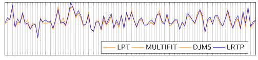
Figure 2: Makespan comparison for 100 instances of class $(3,8,[1,20])$ (x: instances, y: makespan)

By their simple nature the non-ptas algorithms compute solutions even to large instances within a few seconds. While the running time of the ptas is generally on a high level, the increase in the running time as the number of machines and jobs grows is rather small due to the parameterized running time of our algorithm. We emphasize that the running time did not cross the border of $5.6$ hours for any instance computed. We therefore see these experiments as a valid proof of concept for practically feasible ptas’s. The empirical solution quality, although not our main focus, is not superior to the non-ptas algorithms at the considered precision, though the difference is only small. This may be due to the random instances which do not necessarily exhibit a worst-case structure and that the difference in theoretical approximation guarantee is at this state fairly small. We believe that with additional computational resources or further optimizations an even lower precision can be reached, which will lead to a superior solution quality also in experiments.

Appendix A Omitted proofs

See 2.1

Proof A.1.

There are two possible situations to consider: If the makespan does not increase, we have $\mu(\delta)=\mu(\delta_{\text{large}})$. If the makespan increases, consider the loads $\ell_{1},\ldots,\ell_{m}$ of the machines. As the makespan increased, the differences between the loads is bounded by $\varepsilon T$, i. e. $|\ell_{i}-\ell_{i^{\prime}}|\leq\varepsilon T$ for all $i,i^{\prime}$. We thus have $\mu(\delta)-\ell_{i}\leq\varepsilon T$ for all $i$, as $\mu(\delta)=\max_{i}\ell_{i}$. Hence

$$\sum_{j}p_{j}=\sum_{i}\ell_{i}\geq\sum_{i}(\mu(\delta)-\varepsilon T)=m\cdot(\mu(\delta)-\varepsilon T)$$

and thus $(\sum_{j}p_{j})/m\geq\mu(\delta)-\varepsilon T$. As $\operatorname{\text{{opt}}}(J)\geq(\sum_{j}p_{j})/m$, we conclude $\mu(\delta)\leq\operatorname{\text{{opt}}}(J)+\varepsilon T$. The time complexity of $\mathcal{O}((|J_{\text{small}}|+m)\cdot\log(|J_{\text{small}}|+m))$ can be achieved by storing the loads of the machines in a min-heap.

Lemma A.2 (Formal version of Lemma 2.2).

Define $J_{\text{medium}}:=\{j\in J\mid\varepsilon T<p_{j}\leq 2\varepsilon T\}\subseteq J_{\text{large}}$. Let $J_{\text{huge}}=\{j_{1},\ldots,j_{k}\}$ with $p_{j_{1}}\geq p_{j_{2}}\geq\ldots p_{j_{k}}$ and $J_{\text{medium}}=\{j^{\prime}_{1},\ldots,j^{\prime}_{k^{\prime}}\}$ with $p_{j^{\prime}_{1}}\geq p_{j^{\prime}_{2}}\geq\ldots p_{j^{\prime}_{k^{\prime}}}$. Define iteratively $\psi\colon\{1,\ldots,k\}\to\{1,\ldots,k^{\prime},\infty\}$ with $\psi(j)=\min\{j^{\prime}\leq k^{\prime}\mid p_{j}+p_{j^{\prime}}\leq 1\land j^{\prime}\not\in\{\psi(\tilde{j})\mid\tilde{j}<j\}\}$, where $\min\emptyset=\infty$.

There is an optimal schedule $\delta_{\text{large}}$ of $J_{\text{large}}$ such that for each machine $i$ with $\delta_{\text{large}}^{-1}(i)\cap J_{\text{huge}}=\{j\}$, we have either $\delta_{\text{large}}^{-1}(i)=\{j\}$ if $\psi(j)=\infty$ or $\delta_{\text{large}}^{-1}(i)=\{j,\psi(j)\}$ if $\psi(j)<\infty$.

Proof A.3.

Intuitively, $\psi$ maps $j$ to the largest job $j^{\prime}$ in $J_{\text{medium}}$ with which it can be put onto a machine and which is not already mapped to another huge job. If no such job $j^{\prime}$ exists, $\psi(j)=\infty$.

Consider any optimal schedule $\delta_{\text{large}}$ of $J_{\text{large}}$ such that there is a machine $i$ with $\delta_{\text{large}}^{-1}(i)\cap J_{\text{huge}}=\{j\}$ with $\delta_{\text{large}}^{-1}(i)=\{j,j^{\prime}\}$ where either $\psi(j)=\infty$ or $j^{\prime}\neq\psi(j)$. If there are multiple such machines, we consider the one with the job $j=j_{\ell}$ with minimal index in the ordering $j_{1},\ldots,j_{k}$. As $j_{\ell}$ has minimal index, if $\psi(j)=\infty$, all fitting jobs from $J_{\text{medium}}$ are packed with the jobs $j_{1},\ldots,j_{\ell-1}$. Hence, there is no job $j^{\prime}$ that can be packed with $j_{\ell}$. This situation is thus not possible. If $j^{\prime}\neq\psi(j)$, consider the machine $\delta_{\text{large}}(\psi(j)):=i^{\prime}$. As $p_{\psi(j)}+p_{j}\leq 1$ and $p_{\psi(j)}\geq p_{j^{\prime}}$ (by definition of $\psi(j)$), we can exchange $j^{\prime}$ and $\psi(j)$ and still keep a feasible optimal schedule.

Applying the above reason iteratively finally gives us an optimal schedule that always pairs the jobs $j$ and $\psi(j)$ (if $\psi(j)<\infty$).

Lemma A.4 (Formal version of Lemma 2.3).

1. The number of different rounded processing times of $J_{\text{rem}}$ is at most $\lceil 1/\varepsilon\rceil\cdot[\log((1-2\varepsilon)/\varepsilon)+1]$.

2. A schedule $\tilde{\sigma}$ of the rounded processing times implies a schedule $\sigma$ of the original processing time with $\mu(\sigma)\leq(1+\varepsilon)\mu(\tilde{\sigma})$.

3. We have $b_{i,k_{1}}+b_{i,k_{2}}=b_{i+1,(k_{1}+k_{2})/2}$ for all $i$ and all $k_{1},k_{2}$ with $k_{1}\bmod 2=k_{2}\bmod 2$.

Proof A.5.

1. We have $2^{i+1}\varepsilon T=(1-2\varepsilon)T$ iff $i+1=\log((1-2\varepsilon)/\varepsilon)$. For $i>\log((1-2\varepsilon)/\varepsilon)$, there is no job in any interval $I_{i}$. Hence, there are at most $\log((1-2\varepsilon)/\varepsilon)+1$ many values for $i$ such that the processing times lie in $I_{i}$. Every $I_{i}$ is split into $\lceil 1/\varepsilon\rceil+1$ intervals. Hence, there are at most $[\lceil 1/\varepsilon\rceil+1]\cdot[\log((1-2\varepsilon)/\varepsilon)+1]$ many rounded processing times.

2. It is sufficient to show $p_{j}\geq\tilde{p}_{j}\geq(1+\varepsilon)^{-1}p_{j}$. As we only round down, we have $p_{j}\geq\tilde{p}_{j}$ immediately. Let $\tilde{p}_{j}=b_{i,k}$ and hence $p_{j}\in I_{i,k}$. Then

   $$(1+\varepsilon)\tilde{p}_{j}=(1+\varepsilon)b_{i,k}=(1+\varepsilon)[2^{i}\varepsilon T+k\varepsilon^{2}2^{i}T]=$$

   $$2^{i}\varepsilon T+k\varepsilon^{2}2^{i}T+2^{i}\varepsilon^{2}T+k\varepsilon^{3}2^{i}T\geq$$

   $$2^{i}\varepsilon T+k\varepsilon^{2}2^{i}T+2^{i}\varepsilon^{2}T=2^{i}\varepsilon T+(k+1)\varepsilon^{2}2^{i}T=b_{i,k+1}>p_{j}.$$

3. We have

   $$b_{i,k_{1}}+b_{i,k_{2}}=2^{i}\varepsilon T+k_{1}\varepsilon^{2}2^{i}T+2^{i}\varepsilon T+k_{2}\varepsilon^{2}2^{i}T=2^{i+1}\varepsilon T+(k_{1}+k_{2})\varepsilon^{2}2^{i}T.$$

   As $k_{1}\bmod 2=k_{2}\bmod 2$, we have $(k_{1}+k_{2})/2\in\mathbb{Z}_{\geq 0}$ and thus

   $$2^{i+1}\varepsilon T+(k_{1}+k_{2})\varepsilon^{2}2^{i}T=2^{i+1}\varepsilon T+[(k_{1}+k_{2})/2]\varepsilon^{2}2^{i+1}T=b_{i+1,(k_{1}+k_{2})/2}.$$

Proving Lemma 2.4.

To prove Lemma 2.4, we first introduce some notations. For $i^{*},k^{*}_{1},k^{*}_{2}$ with $k^{*}_{1}\bmod 2=k^{*}_{2}\bmod 2$ and, we define the new column $\hat{c}:=\hat{c}(i^{*},k^{*}_{1},k^{*}_{2})\in\hat{\mathcal{C}}$ with (i) $\hat{c}[i,k]=2$, if $i=i^{*}$ and $k=k^{*}_{1}=k^{*}_{2}$ or (ii) $\hat{c}[i,k]=1$, if $i=i^{*}$ and $k\in\{k^{*}_{1},k^{*}_{2}\}$ and $k^{*}_{1}\neq k^{*}_{2}$ or (iii) $\hat{c}[i,k]=-1$, if $i=i^{*}+1$ und $k=(k^{*}_{1}+k^{*}_{2})/2$. In all other cases, we define $\hat{c}[i,k]=0$.

For a subset $\mathcal{C}^{\prime}\subseteq\mathcal{C}$, let $\mathsf{IP}_{\mathcal{C}^{\prime},\hat{\mathcal{C}}}$ be the following integer program:

$$\sum_{c\in\mathcal{C}^{\prime}}x_{c}\leq m;\quad\sum_{c\in\mathcal{C}^{\prime}\cup\hat{\mathcal{C}}}x_{c}\cdot c[i,k]\geq n_{i,k}\ \ \forall(i,k);\quad x_{c}\in\mathbb{Z}_{\geq 0}\ \ \forall c\in\mathcal{C}^{\prime}\cup\hat{\mathcal{C}}$$

Let $\mathsf{IP}_{\mathcal{C}}$ be the original configuration ip. We can now obtain the following switching lemma, which directly implies Lemma 2.4, as a feasible solution $x^{*}$ of $\mathsf{IP}_{\mathcal{C}}$ can be transformed into a feasible solution $y^{*}$ of $\mathsf{IP}_{\mathcal{C}_{\textrm{red}},\hat{\mathcal{C}}}$ and vice versa.

Lemma A.6.

Let $x^{*}$ be a feasible solution of $\mathsf{IP}_{\mathcal{C},\hat{\mathcal{C}}}$.

1. If there is a $c_{1}\in\mathcal{C}$ with $||c_{1}||_{1}>2[\log((1-2\varepsilon)/\varepsilon)+1]$ and $x^{*}_{c_{1}}>0$, there are configurations $c_{2}\in\mathcal{C}$ with $||c_{2}||_{1}<||c_{1}||_{1}$ and $c_{3}\in\hat{\mathcal{C}}$, such that the vector $y$ is a feasible solution of $\mathsf{IP}_{\mathcal{C},\hat{\mathcal{C}}}$ with $y_{c_{1}}=x^{*}_{c_{1}}-1$, $y_{c_{2}}=x^{*}_{c_{2}}+1$, $y_{c_{3}}=1$ and $y_{c}=x^{*}_{c}$ for all other $c$.

2. If there is a configuration $c_{1}=\hat{c}(i^{*},k^{*}_{1},k^{*}_{2})\in\hat{\mathcal{C}}$ with $x^{*}_{c_{1}}>0$ and a configuration $c_{2}\in\mathcal{C}$ with $c_{2}[i^{*}+1,(k^{*}_{1}+k^{*}_{2})/2]=1$ and $x^{*}_{c_{2}}>0$, there is a configuration $c_{3}\in\mathcal{C}$, such that the vector $y$ is a feasible solution of $\mathsf{IP}_{\mathcal{C},\hat{\mathcal{C}}}$ with $y_{c_{1}}=x^{*}_{c_{1}}-1$, $y_{c_{2}}=x^{*}_{c_{2}}-1$, $y_{c_{3}}=x^{*}_{c_{3}}+1$ and $y_{c}=x^{*}_{c}$ for all other $c$.

Proof A.7.

Let $x^{*}$ be a feasible solution of $\mathsf{IP}_{\mathcal{C},\hat{\mathcal{C}}}$.

1. As $||c_{1}||_{1}>2[\log((1-2\varepsilon)/\varepsilon)+1]$, the pidgeonhole principle implies that there are indices $i^{*},k_{1}^{*},k_{2}^{*}$ with $k_{1}^{*}\bmod 2=k_{2}^{*}\bmod 2$, such that $\min\{c_{1}[i^{*},k_{1}^{*}],c_{1}[i^{*},k_{2}^{*}]\}\geq 1$, if $k_{1}^{*}\neq k_{2}^{*}$ or $c_{1}[i^{*},k_{1}^{*}]\geq 2$, if $k_{1}^{*}=k_{2}^{*}$. Choose $c_{3}=\hat{c}(i^{*},k_{1}^{*},k_{2}^{*})$ and $c_{2}=c_{1}-c_{3}$. By construction, we have $c_{2}\in\mathcal{C}$ and $\lVert c_{2}\rVert_{1}=\lVert c_{1}\rVert_{1}+1-2=\lVert c_{1}\rVert_{1}-1$. For $i=i^{*}$ and $k=k^{*}_{1}=k^{*}_{2}$, we have

   $$\sum_{c\in\mathcal{C}^{\prime}\cup\hat{\mathcal{C}}}y_{c}\cdot c[i,k]=\left[\sum_{c\in\mathcal{C}^{\prime}\cup\hat{\mathcal{C}}}x^{*}_{c}\cdot c[i,k]\right]\underbrace{-2}_{\text{by $c_{1}$}}\underbrace{+2}_{\text{by $c_{3}$}}\geq n_{i,k}.$$

   For $i=i^{*}$ and $k^{*}_{1}\neq k^{*}_{2}$ and $k\in\{k^{*}_{1},k^{*}_{2}\}$, we have

   $$\sum_{c\in\mathcal{C}^{\prime}\cup\hat{\mathcal{C}}}y_{c}\cdot c[i,k]=\left[\sum_{c\in\mathcal{C}^{\prime}\cup\hat{\mathcal{C}}}x^{*}_{c}\cdot c[i,k]\right]\underbrace{-1}_{\text{by $c_{1}$}}\underbrace{+1}_{\text{by $c_{3}$}}\geq n_{i,k}.$$

   For $i=i^{*}+1$, and $k=(k^{*}_{1}+k^{*}_{2})/2$, we have

   $$\sum_{c\in\mathcal{C}^{\prime}\cup\hat{\mathcal{C}}}y_{c}\cdot c[i,k]=\left[\sum_{c\in\mathcal{C}^{\prime}\cup\hat{\mathcal{C}}}x^{*}_{c}\cdot c[i,k]\right]\underbrace{+1}_{\text{by $c_{2}$}}\underbrace{-1}_{\text{by $c_{3}$}}\geq n_{i,k}.$$

   Finally, for all other $i$ and $k$, we have

   $$\sum_{c\in\mathcal{C}^{\prime}\cup\hat{\mathcal{C}}}y_{c}\cdot c[i,k]=\sum_{c\in\mathcal{C}^{\prime}\cup\hat{\mathcal{C}}}x^{*}_{c}\cdot c[i,k]\geq n_{i,k},$$

   as nothing changed here.

   As $\sum_{c\in\mathcal{C}}y_{c}=\sum_{c\in\mathcal{C}}x^{*}_{c}\leq m$, we can conclude that $y$ is a feasible solution of $\mathsf{IP}_{\mathcal{C},\hat{\mathcal{C}}}$.

2. Choose $c_{3}=c_{2}-c_{1}$. By construction, we have $c_{3}\in\mathcal{C}$.

   For $i=i^{*}$ and $k=k^{*}_{1}=k^{*}_{2}$, we have

   $$\sum_{c\in\mathcal{C}^{\prime}\cup\hat{\mathcal{C}}}y_{c}\cdot c[i,k]=\left[\sum_{c\in\mathcal{C}^{\prime}\cup\hat{\mathcal{C}}}x^{*}_{c}\cdot c[i,k]\right]\underbrace{+2}_{\text{by $c_{1}$}}\underbrace{-2}_{\text{by $c_{3}$}}\geq n_{i,k}.$$

   For $i=i^{*}$ and $k^{*}_{1}\neq k^{*}_{2}$ and $k\in\{k^{*}_{1},k^{*}_{2}\}$, we have

   $$\sum_{c\in\mathcal{C}^{\prime}\cup\hat{\mathcal{C}}}y_{c}\cdot c[i,k]=\left[\sum_{c\in\mathcal{C}^{\prime}\cup\hat{\mathcal{C}}}x^{*}_{c}\cdot c[i,k]\right]\underbrace{+1}_{\text{by $c_{1}$}}\underbrace{-1}_{\text{by $c_{3}$}}\geq n_{i,k}.$$

   For $i=i^{*}+1$, and $k=(k^{*}_{1}+k^{*}_{2})/2$, we have

   $$\sum_{c\in\mathcal{C}^{\prime}\cup\hat{\mathcal{C}}}y_{c}\cdot c[i,k]=\left[\sum_{c\in\mathcal{C}^{\prime}\cup\hat{\mathcal{C}}}x^{*}_{c}\cdot c[i,k]\right]\underbrace{-1}_{\text{by $c_{2}$}}\underbrace{+1}_{\text{by $c_{3}$}}\geq n_{i,k}.$$

   Finally, for all other $i$ and $k$, we have

   $$\sum_{c\in\mathcal{C}^{\prime}\cup\hat{\mathcal{C}}}y_{c}\cdot c[i,k]=\sum_{c\in\mathcal{C}^{\prime}\cup\hat{\mathcal{C}}}x^{*}_{c}\cdot c[i,k]\geq n_{i,k},$$

   as nothing changed here.

   As $\sum_{c\in\mathcal{C}}y_{c}=\sum_{c\in\mathcal{C}}x^{*}_{c}\leq m$, we can conclude that $y$ is a feasible solution of $\mathsf{IP}_{\mathcal{C},\hat{\mathcal{C}}}$.

Appendix B The complete MILP to optimize the rounding scheme

The $y$-variables can be easily introduced via the big $M$ method and by minimizing the $y$ variables.

$$-\sum_{i\in X^{\prime}}x_{i}+M\cdot y_{X^{\prime}} \leq-1 \forall X^{\prime}\subseteq\{0,\ldots,d-1\}\land|X^{\prime}|=L+1$$

$$(y_{X^{\prime}}=1 \Leftrightarrow\sum_{i\in X^{\prime}}x_{i}\leq 1)$$

We also construct another indicator variable $z_{i_{1},i_{2},i}$ that is $1$ iff $x_{i_{1}}+x_{i_{2}}=x_{i}$ holds.

$$z_{i_{1},i_{2},i}=1 \Leftrightarrow x_{i_{1}}+x_{i_{2}}=x_{i} \forall i_{1},i_{2},i\in\{0,\ldots,d-1\}$$

Again, this implication can be formulated via the big $M$ method or directly by a mixed integer program solver.

Now, we need to guarantee that all configurations containing $L+1$ item sizes can be reduced to $L$ item sizes. Hence, if $y_{X^{\prime}}=1$ this implies that one can get rid of one of the item sizes, i. e. $z_{i_{1},i_{2},i}=1$ for some $i_{1},i_{2}\in X^{\prime}$ and $i\in\{0,\ldots,d-1\}$:

$$y_{X^{\prime}}=1 \implies\exists i^{\prime}_{1},i^{\prime}_{2}\in X^{\prime}\exists i\in\{0,\ldots,r-1\}:z_{i^{\prime}_{1},i^{\prime}_{2},i}=1 \forall X^{\prime}\subseteq\{0,\ldots,d-1\}\land|X^{\prime}|=L+1$$

Again, this implication can be formulated via the big $M$ method or directly by an mixed integer program solver. Finally, the $x_{i}$ are fractional variables and the indicator variables are integral:

$$x_{i} \in[0,1] \forall i\in\{0,\ldots,d-1\}$$

$$y_{X^{\prime}} \in\{0,1\} \forall X^{\prime}\subseteq\{0,\ldots,d-1\}\land|X^{\prime}|=L+1$$

$$z_{i_{1},i_{2},i} \in\{0,1\} \forall i_{1},i_{2},i\in\{0,\ldots,d-1\}$$

In total, we obtain the following mixed integer program:

$$\min \sum_{X^{\prime}}y_{X^{\prime}}+\sum_{i_{1},i_{2},i}z_{i_{1},i_{2},i}\text{ s.t.}$$

$$(1+\varepsilon)x_{0} \geq(1-2\varepsilon)$$

$$x_{0} \leq(1-2\varepsilon)$$

$$x_{d-1} \leq\varepsilon\cdot(1+\varepsilon)$$

$$(1+\varepsilon)x_{i+1} \geq x_{i} \forall i=1,\ldots,d-2$$

$$y_{X^{\prime}}=1 \Leftrightarrow\sum_{i\in X^{\prime}}x_{i}\leq 1$$

$$z_{i_{1},i_{2},i}=1 \Leftrightarrow x_{i_{1}}+x_{i_{2}}=x_{i} \forall i_{1},i_{2},i\in\{0,\ldots,d-1\}$$

$$y_{X^{\prime}}=1 \Rightarrow\exists i^{\prime}_{1},i^{\prime}_{2}\in X^{\prime}\exists i\in\{1,\ldots,n\}:z_{i^{\prime}_{1},i^{\prime}_{2},i}=1 \forall X^{\prime}\subseteq\{0,\ldots,d-1\}\land|X^{\prime}|=L+1$$

$$x_{i} \in[0,1] \forall i\in\{0,\ldots,d-1\}$$

$$y_{X^{\prime}} \in\{0,1\} \forall X^{\prime}\subseteq\{0,\ldots,d-1\}\land|X^{\prime}|=L+1$$

$$z_{i_{1},i_{2},i} \in\{0,1\} \forall i_{1},i_{2},i\in\{0,\ldots,d-1\}$$

Appendix C Computing Multi-Dimensional Convolutions with FFT

The JR-algorithm depends on multiplying multi-variate polynomials. Here we describe how to do this using the well-known fast Fourier transformation (fft). We start by introducing multi-dimensional polynomials as well as multi-dimensional discrete Fourier transformations (dfts).

Definition C.1.

A multivariate or multi-dimensional polynomial $p$ of $d$ variables $x_{1},\dots,x_{d}$ and coordinate degree $n=(n_{1},\dots,n_{d})$ is a linear combination of monomials, i.e.

$$p(x)=\sum_{k\leq n-\mathbf{1}}p_{k}x^{k}\qquad\text{where}\quad x^{k}:=\prod_{j=1}^{d}x_{j}^{k_{j}}\quad\forall k\in\{0,\dots,n_{1}-1\}\times\dots\times\{0,\dots,n_{d}-1\},$$

$n-\mathbf{1}=(n_{1}-1,\dots,n_{d}-1)$, and $p_{k}\in\mathbb{C}$ f.a. $k\leq n-\mathbf{1}$. So $p$ is a (univariate) polynomial of degree $n_{j}$ in each coordinate direction $j$.

Definition C.2.

For two multivariate polynomials $f(x)=\sum_{k\leq n-\mathbf{1}}f_{k}x^{k}$, $g(x)=\sum_{k\leq n-\mathbf{1}}g_{k}x^{k}$ the multi-dimensional discrete convolution $(f*g)(x)=\sum_{k\leq 2n-\mathbf{2}}c_{k}x^{k}$ of $f$ and $g$ is defined by

$$c_{k}=\sum_{j\leq k}f_{j}\cdot g_{k-j},\quad\text{i.e.}\quad c_{(k_{1},\dots,k_{d})}=\sum_{j_{1}=0}^{k_{1}}\sum_{j_{2}=0}^{k_{2}}\dots\sum_{j_{d}=0}^{k_{d}}f_{(j_{1},\dots,j_{d})}\cdot g_{(k_{1}-j_{1},\dots,k_{d}-j_{d})}.$$

Hence, a truly primitive approach to compute $f*g$ takes time $\mathcal{O}(\sum_{k\leq 2n-\mathbf{2}}\prod_{j=1}^{d}(k_{j}+1))\leq\mathcal{O}(2^{d}N^{2})$ where $N=\prod_{j=1}^{d}n_{j}$ is the number of all input points.

However, the convolution theorem says that $\mathcal{F}\{f*g\}=N\cdot\mathcal{F}\{f\}\odot\mathcal{F}\{g\}$ where $\mathcal{F}$ denotes the Fourier transform operator and $\odot$ denotes the point-wise multiplication, i.e. $(v\odot w)_{k}=v_{k}\cdot w_{k}$. Therefore, one can compute the convolution $f*g$ by computing

$$f*g=\mathcal{F}^{-1}\{N\cdot\mathcal{F}\{f\}\odot\mathcal{F}\{g\}\}.$$

For our goals we only depend on the discrete Fourier transformation as follows.

Definition C.3 ( discrete Fourier transformation (dft)).

The multi-dimensional discrete Fourier transformation (dft) $\hat{f}=\mathcal{F}\{f\}$ of $f$ is defined by

$$\hat{f}_{k}=\sum_{\ell\leq n-\mathbf{1}}f_{\ell}\cdot\exp\left(-i2\pi\sum_{j=1}^{d}\frac{k_{j}\ell_{j}}{n_{j}}\right)\quad\forall k\leq n-\mathbf{1}$$

whereas the inverse multi-dimensional dft $\mathcal{F}^{-1}\{\hat{f}\}$ of $\hat{f}$ is given by

$$f_{k}=\frac{1}{N}\sum_{\ell\leq n-\mathbf{1}}\hat{f}_{\ell}\cdot\exp\left(i2\pi\sum_{j=1}^{d}\frac{k_{j}\ell_{j}}{n_{j}}\right)\quad\forall k\leq n-\mathbf{1}.$$

To give more light to these definitions let us consider the $1$-dimensional case, i.e. $d=1,n=n_{1}$. Then Definition C.3 simplifies to

$$\hat{f}_{k}=\sum_{\ell=0}^{n-1}f_{\ell}\cdot e^{-i2\pi k\ell/n}\quad\text{and}\quad f_{k}=\frac{1}{n}\sum_{\ell=0}^{n-1}\hat{f}_{\ell}\cdot e^{i2\pi k\ell/n}\quad\forall k=0,\dots,n-1.$$

Obviously, since $\hat{f}_{k}=f(e^{-i2\pi k/n})$ for $k=0,\dots,n-1$ one can compute the dft of $f$ in time $\mathcal{O}(n^{2})$ by simply evaluating $f$ in $n$ points. Fortunately, this running time can be reduced to $\mathcal{O}(n\log n)$ by algorithmically exploiting the fact, that the evaluation of

$$f(x)\;=\;(f_{0}x^{0}+f_{2}x^{2}+\dots)+x\cdot(f_{1}x^{0}+f_{3}x^{2}+\dots)\;=\;p(x^{2})+x\cdot q(x^{2})$$

can always be written by the evaluation of two polynomials $p,q$ of half-sized degrees for any input point $x$. This running time improvement is the reason to call a dft an fft. Also the inverse can be computed efficiently by using just the same trick, since $f_{k}=\frac{1}{n}\hat{f}(e^{i2\pi k/n})$. See Fig. 3 for an illustration of the whole computation.

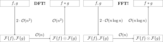
Figure 3: Computing a 1D-convolution with discrete/fast Fourier transformations

Finally, turning back to the general case $n=(n_{1},\dots,n_{d})$ we can compute the multi-dimensional fft of $f$ by computing $1$-dimensional ffts. In more detail, we may divide the whole computation into $N/n_{j}$ $1$-dimensional transformations of size $n_{j}$ for each coordinate direction $j$. This yields the usual running time of

$$\sum_{j=1}^{d}\frac{N}{n_{j}}\mathcal{O}(n_{j}\log n_{j})=\mathcal{O}(N\sum_{j=1}^{d}\log n_{j})=\mathcal{O}(N\log N).$$

Appendix D Computational Results for E3, E4, and BIG

Table 5: Computational results for the classes of family E3

family	$m$	$n$	$U$	better	equal	avg_quot	avg_time
E3	$10$	$31$	$[100,200]$	$0$	$0$	$1.07$	$182$
E3	$10$	$31$	$[1,100]$	$0$	$0$	$1.08$	$82$
E3	$10$	$32$	$[100,200]$	$0$	$2$	$1.07$	$179$
E3	$10$	$32$	$[1,100]$	$0$	$0$	$1.09$	$81$
E3	$10$	$41$	$[100,200]$	$0$	$0$	$1.07$	$214$
E3	$10$	$41$	$[1,100]$	$0$	$0$	$1.09$	$80$
E3	$10$	$42$	$[100,200]$	$0$	$0$	$1.07$	$220$
E3	$10$	$42$	$[1,100]$	$0$	$0$	$1.1$	$82$
E3	$10$	$51$	$[100,200]$	$0$	$0$	$1.08$	$225$
E3	$10$	$51$	$[1,100]$	$0$	$0$	$1.1$	$80$
E3	$10$	$52$	$[100,200]$	$0$	$0$	$1.06$	$224$
E3	$10$	$52$	$[1,100]$	$0$	$0$	$1.09$	$75$
E3	$3$	$10$	$[100,200]$	$4$	$15$	$1.03$	$114$
E3	$3$	$10$	$[1,100]$	$3$	$21$	$1.03$	$67$
E3	$3$	$11$	$[100,200]$	$21$	$2$	$1.02$	$150$
E3	$3$	$11$	$[1,100]$	$4$	$20$	$1.03$	$61$
E3	$3$	$13$	$[100,200]$	$20$	$7$	$1.03$	$133$
E3	$3$	$13$	$[1,100]$	$4$	$15$	$1.03$	$60$
E3	$3$	$14$	$[100,200]$	$20$	$1$	$1.03$	$146$
E3	$3$	$14$	$[1,100]$	$6$	$7$	$1.03$	$62$
E3	$3$	$16$	$[100,200]$	$30$	$2$	$1.02$	$166$
E3	$3$	$16$	$[1,100]$	$9$	$13$	$1.03$	$67$
E3	$3$	$17$	$[100,200]$	$7$	$1$	$1.03$	$146$
E3	$3$	$17$	$[1,100]$	$5$	$11$	$1.03$	$59$
E3	$5$	$16$	$[100,200]$	$1$	$1$	$1.05$	$135$
E3	$5$	$16$	$[1,100]$	$0$	$3$	$1.06$	$66$
E3	$5$	$17$	$[100,200]$	$8$	$2$	$1.03$	$149$
E3	$5$	$17$	$[1,100]$	$2$	$4$	$1.05$	$68$
E3	$5$	$21$	$[100,200]$	$19$	$3$	$1.02$	$184$
E3	$5$	$21$	$[1,100]$	$1$	$0$	$1.06$	$65$
E3	$5$	$22$	$[100,200]$	$4$	$2$	$1.04$	$178$
E3	$5$	$22$	$[1,100]$	$1$	$1$	$1.06$	$63$
E3	$5$	$26$	$[100,200]$	$11$	$1$	$1.04$	$185$
E3	$5$	$26$	$[1,100]$	$2$	$2$	$1.06$	$67$
E3	$5$	$27$	$[100,200]$	$1$	$0$	$1.05$	$166$
E3	$5$	$27$	$[1,100]$	$2$	$1$	$1.05$	$67$
E3	$8$	$25$	$[100,200]$	$1$	$0$	$1.06$	$176$
E3	$8$	$25$	$[1,100]$	$0$	$0$	$1.07$	$74$
E3	$8$	$26$	$[100,200]$	$0$	$0$	$1.06$	$177$
E3	$8$	$26$	$[1,100]$	$0$	$0$	$1.07$	$81$
E3	$8$	$33$	$[100,200]$	$0$	$1$	$1.06$	$202$
E3	$8$	$33$	$[1,100]$	$0$	$0$	$1.09$	$72$
E3	$8$	$34$	$[100,200]$	$1$	$0$	$1.06$	$195$
E3	$8$	$34$	$[1,100]$	$0$	$0$	$1.08$	$78$
E3	$8$	$41$	$[100,200]$	$0$	$0$	$1.06$	$207$
E3	$8$	$41$	$[1,100]$	$0$	$0$	$1.08$	$76$
E3	$8$	$42$	$[100,200]$	$0$	$0$	$1.06$	$211$
E3	$8$	$42$	$[1,100]$	$0$	$0$	$1.08$	$77$

Table 6: Computational results for the classes of family E4

family	$m$	$n$	$U$	better	equal	avg_quot	avg_time
E4	$2$	$10$	$[1,20]$	$4$	$61$	$1.01$	$39$
E4	$2$	$10$	$[1,100]$	$14$	$21$	$1.01$	$48$
E4	$2$	$10$	$[20,50]$	$10$	$12$	$1.02$	$46$
E4	$2$	$10$	$[50,100]$	$14$	$9$	$1.03$	$59$
E4	$2$	$10$	$[100,200]$	$15$	$3$	$1.02$	$71$
E4	$2$	$10$	$[100,800]$	$14$	$8$	$1.01$	$97$
E4	$3$	$9$	$[1,20]$	$0$	$43$	$1.03$	$37$
E4	$3$	$9$	$[1,100]$	$6$	$29$	$1.03$	$57$
E4	$3$	$9$	$[20,50]$	$2$	$9$	$1.05$	$61$
E4	$3$	$9$	$[50,100]$	$2$	$0$	$1.05$	$75$
E4	$3$	$9$	$[100,200]$	$2$	$0$	$1.05$	$95$
E4	$3$	$9$	$[100,800]$	$5$	$14$	$1.03$	$132$

Table 7: Computational results for the classes of the additional family BIG

family	$m$	$n$	$U$	better	equal	avg_quot	avg_time
BIG	$25$	$100$	$[1,1000]$	$0$	$0$	$1.13$	$171$
BIG	$50$	$200$	$[1,1000]$	$0$	$0$	$1.14$	$172$
BIG	$75$	$300$	$[1,1000]$	$0$	$0$	$1.14$	$179$
BIG	$100$	$400$	$[1,1000]$	$0$	$0$	$1.15$	$180$

References

- [1] Noga Alon, Yossi Azar, Gerhard J. Woeginger, and Tal Yadid. Approximation schemes for scheduling. In Michael E. Saks, editor, Proceedings of the Eighth Annual ACM-SIAM Symposium on Discrete Algorithms, 5-7 January 1997, New Orleans, Louisiana, USA, pages 493–500. ACM/SIAM, 1997. URL: http://dl.acm.org/citation.cfm?id=314161.314371.
- [2] József Beck and Tibor Fiala. “Integer-making” theorems. Discrete Applied Mathematics, 3(1):1–8, 1981.
- [3] Debe Bednarchak and Martin Helm. A note on the beck-fiala theorem. Combinatorica, 17(1):147–149, 1997.
- [4] Édouard Bonnet and Florian Sikora. The PACE 2018 parameterized algorithms and computational experiments challenge: The third iteration. In IPEC, volume 115 of LIPIcs, pages 26:1–26:15. Schloss Dagstuhl - Leibniz-Zentrum für Informatik, 2018.
- [5] Vincent Bouchitté and Ioan Todinca. Listing all potential maximal cliques of a graph. Theor. Comput. Sci., 276(1-2):17–32, 2002.
- [6] Holger Dell, Christian Komusiewicz, Nimrod Talmon, and Mathias Weller. The PACE 2017 parameterized algorithms and computational experiments challenge: The second iteration. In IPEC, volume 89 of LIPIcs, pages 30:1–30:12. Schloss Dagstuhl - Leibniz-Zentrum für Informatik, 2017.
- [7] M. Ayaz Dzulfikar, Johannes Klaus Fichte, and Markus Hecher. The PACE 2019 parameterized algorithms and computational experiments challenge: The fourth iteration (invited paper). In IPEC, volume 148 of LIPIcs, pages 25:1–25:23. Schloss Dagstuhl - Leibniz-Zentrum für Informatik, 2019.
- [8] Friedrich Eisenbrand and Robert Weismantel. Proximity results and faster algorithms for integer programming using the steinitz lemma. ACM Trans. Algorithms, 16(1):5:1–5:14, 2020.
- [9] Matteo Frigo and Steven G. Johnson. The design and implementation of FFTW3. Proceedings of the IEEE, 93(2):216–231, 2005.
- [10] Ronald L. Graham. Bounds on multiprocessing timing anomalies. SIAM Journal of Applied Mathematics, 17(2):416–429, 1969.
- [11] J. N. D. Gupta and A. J. Ruiz-Torres. A listfit heuristic for minimizing makespan on identical parallel machines. Production Planning & Control, 12(1):28–36, 2001.
- [12] Jatinder ND Gupta and Alex J Ruiz-Torres. A listfit heuristic for minimizing makespan on identical parallel machines. Production Planning & Control, 12(1):28–36, 2001.
- [13] Dorit S. Hochbaum and David B. Shmoys. Using dual approximation algorithms for scheduling problems theoretical and practical results. J. ACM, 34(1):144–162, 1987.
- [14] Klaus Jansen, Kim-Manuel Klein, and José Verschae. Closing the gap for makespan scheduling via sparsification techniques. Math. Oper. Res., 45(4):1371–1392, 2020. doi:10.1287/moor.2019.1036.
- [15] Klaus Jansen, Alexandra Lassota, and Lars Rohwedder. Near-linear time algorithm for n-fold ilps via color coding. In Proc. ICALP 2019, pages 75:1–75:13, 2019.
- [16] Klaus Jansen and Lars Rohwedder. On integer programming and convolution. In Proc. ITCS 2019, pages 43:1–43:17, 2019.
- [17] Edward G. Coffman Jr., M. R. Garey, and David S. Johnson. An application of bin-packing to multiprocessor scheduling. SIAM J. Comput., 7(1):1–17, 1978.
- [18] Hendrik W. Lenstra Jr. Integer programming with a fixed number of variables. Math. Oper. Res., 8(4):538–548, 1983.
- [19] Ravi Kannan. Minkowski’s convex body theorem and integer programming. Math. Oper. Res., 12(3):415–440, 1987.
- [20] SK Kedia. A job scheduling problem with parallel processors. Unpublished report, Department of Industrial and Operations Engineering. University of Michigan, Ann Arbor, MI, 1971.
- [21] Martin Koutecký, Asaf Levin, and Shmuel Onn. A parameterized strongly polynomial algorithm for block structured integer programs. In ICALP, volume 107 of LIPIcs, pages 85:1–85:14. Schloss Dagstuhl - Leibniz-Zentrum für Informatik, 2018.
- [22] Abey Kuruvilla and Giuseppe Paletta. Minimizing makespan on identical parallel machines. Int. J. Oper. Res. Inf. Syst., 6(1):19–29, 2015.
- [23] Chung-Yee Lee and J. David Massey. Multiprocessor scheduling: combining LPT and MULTIFIT. Discret. Appl. Math., 20(3):233–242, 1988.
- [24] Joseph Y.-T. Leung. Bin packing with restricted piece sizes. Inf. Process. Lett., 31(3):145–149, 1989. doi:10.1016/0020-0190(89)90223-8.
- [25] Dániel Marx. Parameterized complexity and approximation algorithms. Comput. J., 51(1):60–78, 2008. doi:10.1093/comjnl/bxm048.
- [26] Bárbara Rodeker, M. Virginia Cifuentes, and Liliana Favre. An empirical analysis of approximation algorithms for euclidean TSP. In Hamid R. Arabnia, editor, Proceedings of the 2009 International Conference on Scientific Computing, CSC 2009, July 13-16, 2009, Las Vegas, Nevada, USA, pages 190–196. CSREA Press, 2009.
- [27] Frances Rosamond. Parameterized complexity-news. The Newsletter of the Parameterized Complexity Community Volume, 2006.
- [28] Hisao Tamaki. Positive-instance driven dynamic programming for treewidth. J. Comb. Optim., 37(4):1283–1311, 2019.
- [29] Minyi Yue. On the exact upper bound for the multifit processor scheduling algorithm. Annals of Operations Research, 24(1):233–259, 1990.