The Solar Memory From Hours to Decades

Abstract

Waiting time distributions allow us to distinguish at least three different types of dynamical systems, such as (i) linear random processes (with no memory); (ii) nonlinear, avalanche-type, nonstationary Poisson processes (with memory during the exponential growth of the avalanche rise time); and (iii) chaotic systems in the state of a nonlinear limit cycle (with memory during the oscillatory phase). We describe the temporal evolution of the flare rate $\lambda(t)\propto t^{p}$ with a polynomial function, which allows us to distinguish linear ($p\approx 1$) from nonlinear ($p\lower 1.72218pt\hbox{$\;\buildrel>\over{\scriptstyle\sim}\;$}2$) events. The power law slopes $\alpha$ of observed waiting times (with full solar cycle coverage) cover a range of $\alpha=2.1-2.4$, which agrees well with our prediction of $\alpha=2.0+1/p=2.3-2.5$. The memory time can also be defined with the time evolution of the logistic equation, for which we find a relationship between the nonlinear growth time $\tau_{G}=\tau_{rise}/(4p)$ and the nonlinearity index $p$. We find a nonlinear evolution for most events, in particular for the clustering of solar flares ($p=2.2\pm 0.1$), partially occulted flare events ($p=1.8\pm 0.2$), and the solar dynamo ($p=2.8\pm 0.5$). The Sun exhibits memory on time scales of $\;\buildrel<\over{\scriptstyle\sim}\;$2 hours to 3 days (for solar flare clustering), 6 to 23 days (for partially occulted flare events), and 1.5 month to 1 year (for the rise time of the solar dynamo).

1 Introduction

The simplest timing information we can obtain from astrophysical data is probably an event catalog that contains the (start or peak) times $t_{i}$ of some phenomenon, such as solar or stellar flares, observed at some chosen wavelength. An immediate derivation of this parameter is the so-called waiting time $\tau=t_{i+1}-t_{i}$ (also called interval time, elapsed time, or laminar time). From the statistical analysis of such data we can distinguish between at least three different dynamical systems: linear random processes, nonlinear (avalanche) processes, and oscillatory chaotic systems in the state of limit cycles. The dynamical properties of these three types of systems is manifested in their waiting time distributions: (i) linear (stationary) random processes exhibit exponentially dropping-off distribution functions; (ii) nonlinear (nonstationary Poissonian) processes display power law-like distribution functions; and (iii) chaotic systems with oscillatory limit-cycle behavior reveal periodic processes. Another distinguishing criterion is their “memory” capability: (i) random processes are incoherent and have no memory in consecutive random fluctuations; (ii) nonlinear (avalanche) events are typically exponentially growing and have a memory for the duration of their rise time; (iii) while (chaotic) limit-cycle behavior has a memory that lasts at least as long as the oscillatory phase. Needless to say that the observational and statistical analysis of such systems has far-reaching consequences in identifying and modeling the underlying physical mechanisms.

Analysis of waiting time distributions and interpretations in terms of nonlinear system dynamics has been explored mostly in solar flare data sets (Wheatland et al. 1998; Boffetta et al. 1999; Wheatland 2000a; Leddon 2001; Lepreti et al. 2001; Norman et al. 2001; Wheatland and Litvinenko 2002; Grigolini et al. 2002; Aschwanden and McTiernan 2010; Gorobets and Messerotti 2012; Hudson 2020; Morales and Santos 2020). Similar waiting time distributions have been found in other solar data sets, such as in coronal mass ejections (Wheatland 2003; Yeh et al. 2005; Wang et al. 2013, 2017); in solar energetic particle events (Li et al. 2014); in solar wind discontinuities and its intermittent turbulence (Greco et al. 2009; Wanliss and Weygand 2007), in heliospheric type III radio burst storms (Eastwood et al. 2010), and in solar wind switchback events (Bourouaine et al. 2020; Dudok de Wit et al. 2020; Aschwanden and Dudok de Wit 2021). The cyclic behavior of the solar dynamo has been established over millennia (Usoskin et al. 2017). Extending out to stars, waiting time distributions were studied in active and inactive M-dwarf stars (Hawley et al. 2014; Li et al. 2018), in the avalanche dynamics of radio pulsar glitches and in gamma-ray bursts (Guidorzi et al. 2015; Yi et al. 2016), and black hole systems (Wang et al. 2015, 2017).

It was recognized that a deeper understanding of waiting time distributions requires a physically motivated model of the variability of the flare rate function. However, the power law slope $\alpha$ of waiting time distributions, $N(\tau)\propto\tau^{-\alpha}$, does not exhibit a unique value, but is found to vary in a range of $1\lower 1.72218pt\hbox{$\;\buildrel<\over{\scriptstyle\sim}\;$}\alpha\lower 1.72218pt\hbox{$\;\buildrel<\over{\scriptstyle\sim}\;$}3$ (Wheatland and Litvinenko 2002; Aschwanden and McTiernan 2010). It was noted that the variability of the flare rate strongly depends on the phase of the solar cycle (Aschwanden and Dudok de Wit 2021; Aschwanden, Johnson, and Nurhan 2021).

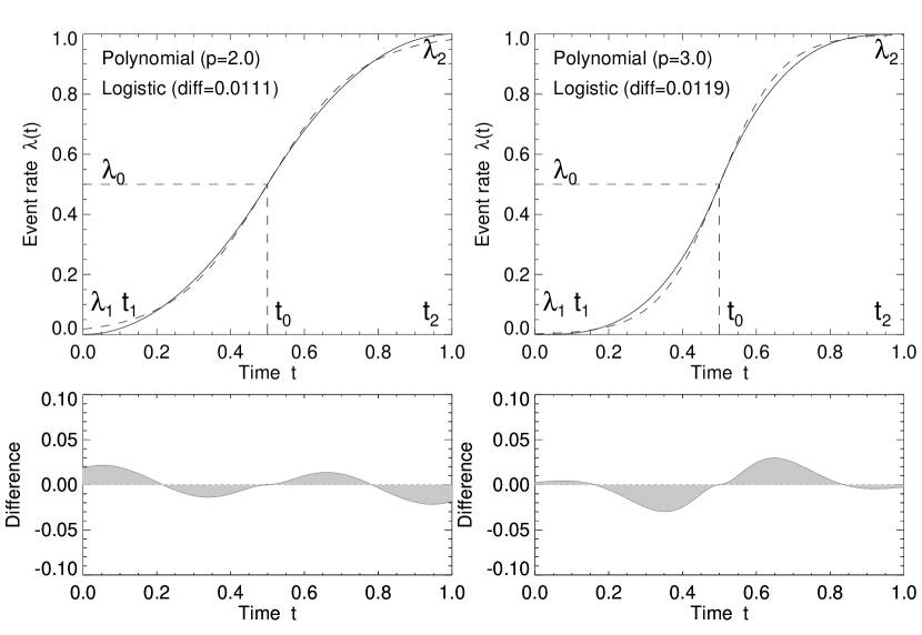
Figure 1: The time profile of a flare rate function $\lambda)(t)$ is modeled with polynomial functions (Eq. 6), here with a quadratic function, $\lambda_{pol}(t)\propto t^{p}$, with $p=2$ (left; solid curve), and with a cubic function, $\lambda_{pol}(t)\propto t^{3}$, with $p=3$ (right; solid curve). Alternatively, the time profile $\lambda_{log}$ is modeled with the logistic equation (Eq. 8) (dashed curve), consisting of an initial exponential rise phase with subsequent saturation. The rise time is defined within the time range of $[t_{1},t_{2}]$. The logistic model is almost identical to the polynomial model, with a mean difference of $|\lambda_{log}(t)-\lambda_{pol}(t)|\approx 1\%$.

In this study we focus on the “memory” of solar processes, which we characterize with the duration of coherent growth in solar time structures. We model the time evolution of the event rate during the initial exponential growth phase with a polynomial function, $\lambda(t)\propto t^{p}$. This coherent growth phase is also typical for avalanching events that occur in self-organized criticality models (Aschwanden 2011). The time evolution of avalanching flare rates can also be described with the logistic first-order differential equation (Aschwanden et al. 1998, Wang et al. 2009; Aschwanden 2012b; Qin and Wu 2018), which is almost identical to the polynomial model (see comparisons in Fig. 1). We measure the degree of nonlinearity, which controls the coherent evolution during the rise time of an instability, and find that the Sun has a memory over time scales varying by at least four orders of magnitude, from clustering of solar flares (on time scales of $\lower 1.72218pt\hbox{$\;\buildrel<\over{\scriptstyle\sim}\;$}2$ hours) to the dynamo-driven solar cycle (on time scales of several decades).

The content of this paper includes a brief description of the theory (Section 2), data analysis of GOES data (Section 3), a discussion of previous work (Section 4), and conclusions (Section 5).

2 Theory

2.1 The Waiting Time Distribution

Waiting time distributions, $N(\tau)\ d\tau$, have the diagnostic potential to reveal whether solar flares are generated by a stochastic (or random) stationary Poisson process (if they obey an exponential distribution, $N(\tau)\propto\exp[-\tau]$), or by a nonstationary (nonlinear) Poission process (if they obey a power law-like distribution, $N(\tau)\propto\tau^{-\alpha}$) (Wheatland and Litvinenko 2002). The difference between a stationary and a nonstationary Poisson process is generally quantified by the statistical behavior of the flare rate function $\Lambda(t)$, which can be constant, i.e., $\Lambda(t)=\Lambda_{0}$, at one extreme, or can be highly time-variable, following an arbitrary temporal function $\Lambda(t)$, in the other extreme. Observations generally exhibit nonstationary flare rate functions, $\Lambda(t)\neq const$ (Wheatland et al. 1998; Wheatland 2000c; 2006; Wheatland and Litvinenko 2002; Aschwanden and McTiernan 2010; Aschwanden 2019b). While we denote the entirely observed time profile of the flare rate with the symbol $\Lambda(t)$, time segments of coherent growth are denoted with the symbol $\lambda(t)$. Various analytical incarnations of the flare rate function $\lambda(t)$ have been used to calculate waiting time distributions, such as a polynomial function $\lambda(t)\propto t^{p}$, a sinusoidal function $\lambda(t)\propto\sin(t)^{p}$, or a gaussian function $\lambda(t)\propto\exp(-t^{2})$, for which exact analytical solutions were found recently, in terms of Bessel functions (Nurhan et al. 2021) and the incomplete gamma function (Aschwanden, Johnson, and Nurhan 2021).

The power law slope $\alpha$ of waiting time distributions, $N(\tau)\propto\tau^{-\alpha}$, does not exhibit a unique value, but is found to vary in a range of $1\lower 1.72218pt\hbox{$\;\buildrel<\over{\scriptstyle\sim}\;$}\alpha\lower 1.72218pt\hbox{$\;\buildrel<\over{\scriptstyle\sim}\;$}3$ (Wheatland and Litvinenko 2002; Aschwanden and McTiernan 2010). This variable behavior was attributed to intrinsically different flare rate evolutions $\lambda(t)$ during the solar cycle minimum and maximum phase (Wheatland and Litvinenko 2002). More specifically, recent work has shown that the power law slope $\alpha$ of waiting time distributions depends on the nonlinearity index $p(\alpha)$ of the polynomial flare rate evolution $\lambda(t)\propto t^{p}$ in a unique way (Aschwanden, Johnson, and Nurhan 2021),

$$\alpha=2+{1\over p}\ ,$$ (1)

based on the calculation of the exact analytical solution in terms of the incomplete Gamma function $\gamma[\alpha,\beta]$, with $\alpha$ the power law slope of the waiting time distribution, and with the argument $\beta=\lambda_{0}\tau$, where $\lambda_{0}$ is the mean flare rate and $\tau$ is the waiting time,

$$N(\tau,\alpha)\ d\tau=\lambda_{0}(\alpha-1)\ \gamma[\alpha,\beta=\lambda_{0}\tau]\ (\lambda_{0}\tau)^{-\alpha}\ d\tau\ .$$ (2)

A practical approximation is an expression in terms of the Gamma function $\Gamma[\alpha]$,

$$N(\tau,\alpha)\ d\tau=\lambda_{0}(\alpha-1)\ \Gamma[\alpha]\ (\lambda_{0}\tau)^{-\alpha}\ d\tau\ ,$$ (3)

which leads to a straight power law, $N(\tau)\propto\tau^{-\alpha}$, and agrees with the exact analytical solution in the asymptotic limit of large waiting times. Note that the definition of the Gamma function entails an integral with the limits $[0,\infty]$, while the incomplete Gamma function has finite integral limits $[0,\beta]$ (see Eqs. (20) and (24) in Aschwanden et al. 2021), and applies in the asymptotic regime $\lambda_{0}\tau\gg 1$ where a power law function is found.

2.2 The Polynomial Flare Rate Function

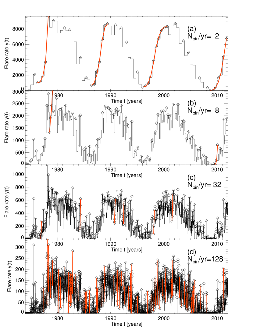
Figure 2: Time profile (histograms) of the flare rate $\Lambda(t)$ during the time range of 37 years (1974-2012) with four different time resolutions of 2 (a), 8 (b), 32 (c), and 128 bins per year (d). The red curves represent best fits of the polynomial flare rate function $\lambda(t)$. The local peaks of the histograms are marked with diamonds.

As we will see in the following, waiting time distributions can only be understood with the knowledge of the temporal variability of the flare rate. The variability of the flare rate can most easily be quantified by histograms. Such a histogram of the flare rate $\Lambda(t)$ is shown in Fig. 2a, with four different time resolutions, expressed by the time bin widths $\Delta t$ = (1 year)/$n_{bin}$ for $n_{bin}=2$ (Fig. 2a), $n_{bin}=8$ (Fig. 2b), $n_{bin}=32$ (Fig. 2c), and $n_{bin}=128$ (Fig. 2d). The histograms are sampled from the entire data set of 338,661 flare events during 37 years (1974-2012). The time profile $\Lambda(t)$ shown in Fig. 2 reveals four major time structures at low time resolution (Fig. 2a), each one encompassing a time duration of $\approx 11$ years, which obviously are attributed to the magnetic (Hale) solar cycle (Fig. 2a). The shorter time structures, visible at higher time resolution (Figs. 2c, and 2d), contain either random noise, nonlinear clustering of flares (indicating a “solar memory”), or a combination of both, which is one of the main tasks pursued in this study.

In a next step we define time structures $\lambda(t)$. They represent partial time segments and are extracted from the entire time profile $\Lambda(t)$ extending over the total (37-year) time interval of the observed flare rates. A first selection criterion of time structures is made by requiring a local peak $\lambda(t=t_{max})$ in the time profile $\Lambda(t)$,

$$\lambda(t_{i-1})<\lambda(t_{i})=\lambda(t=t_{max})>\lambda(t_{i+1})\ .$$ (4)

Secondly, we define the absolute minimum $t_{min}$ between two subsequent peaks,

$$\lambda(t_{max,j-1})>\lambda(t=t_{min})<\lambda(t_{max,j+1})\ .$$ (5)

The time interval between a minimum at $t_{min}$ and a maximum at $t_{max}$ is characterized by a monotonic increase in the flare rate. The simplest definition of a time structure would be a linear segment from $\lambda_{min}=\lambda(t=t_{min})$ to $\lambda_{max}=\lambda(t=t_{max})$. However, in order to make our time structures capable to distinguish between linear and nonlinear time structures, we generalize the linear exponent $p=1$ to a nonlinearity index $p\geq 1$,

$$\lambda(t)=\left\{\begin{array}[]{ll}\lambda_{1}+(\lambda_{0}-\lambda_{1})\left[{(t-t_{1})/(t_{0}-t_{1})}\right]^{p}&\quad{\rm for}\ t_{1}\leq t\leq t_{0}\\ \lambda_{2}+(\lambda_{0}-\lambda_{2})\left[{(t_{2}-t)/(t_{2}-t_{0})}\right]^{p}&\quad{\rm for}\ t_{0}\leq t\leq t_{2}\\ \end{array}\right.\ .$$ (6)

A graphical definition of such a rise time structure is shown in Fig. 1, which covers a time interval of $[t_{1},t_{2}]=[t_{min},t_{max}]$, and has an inflection point at $[t_{0},\lambda_{0}]$. Note that the time profile in the time range $t_{1}\leq t\leq t_{2}$ before the inflection point at $t_{0}$ is identical with the polynomial definition in Aschwanden et al. (2021). Such a time structure is defined by 7 parameters: by four constants $[t_{1},t_{2},\lambda_{1},\lambda_{2}]$ and three free parameters $[t_{0},\lambda_{0},p]$, where $[t_{0},\lambda_{0}]$ define the inflection point and $p$ is the nonlinearity index. Since there are 3 free parameters we require at least 4 or 5 time bins per fitted time structure.

This definition of time structures has the capability to discriminate between linear $(p=1)$ and nonlinear $(p\lower 1.72218pt\hbox{$\;\buildrel>\over{\scriptstyle\sim}\;$}2)$ time evolutions. Furthermore, it reveals time structures in a large range of time resolutions, but is far from complete event detection, especially for noisy structures with a duration of less than 4 to 5 time bins. Thus, this event detection algorithm is biased towards long-duration time structures, but should not be biased with respect to linear versus nonlinear event statistics.

2.3 The Logistic Flare Rate Function

In the previous section we defined the polynomial flare rate function $\lambda(t)$, which provides us a diagnostic whether the flare rate is stochastic, without any memory (if $p\approx 1$), or has some memory (if $p\lower 1.72218pt\hbox{$\;\buildrel>\over{\scriptstyle\sim}\;$}2$). A time structure is defined here by a time interval with coherent growth in the event rate. Our parameterization in terms of a polynomial index $p$, i.e., $\lambda(t)\propto t^{p}$, was chosen mostly for reasons of mathematical convenience, and has been used in a previous publication (Aschwanden, Johnson, and Nurhan 2021). Alternatively, we find that the time evolution of the flare rate can be represented with a physical model of logistic growth and saturation, which moreover is almost indistinguishable from the polynomial model of the flare rate evolution (Fig. 1).

The time evolution of the logistic growth model (Aschwanden 2011, p.94) is universally similar for many instabilities, consisting of an initial exponential growth phase with subsequent saturation, which can be described by a simple first-order differential equation (discovered by Pierre François Verhulst in 1845; May 1974; Beltrami 1987, Jackson 1989, Aschwanden 2011, p.94),

$${d\lambda(t)\over dt}=\left({\lambda(t)\over\tau_{G}}\right)\left(1-{\lambda(t)\over\lambda_{\infty}}\right)\ ,$$ (7)

where $\lambda(t)$ is the time-dependent event rate here, $\lambda_{\infty}$ is the maximum rate asymptotically reached at infinite time $t\mapsto\infty$ (also called the carrying capacity in ecological applications), and $\tau_{G}$ is the e-folding (exponential) growth time. In our application here, $\lambda(t)$ is the time-dependent event rate that monotonically increases during the rise time of an instability, which is a phase of coherent growth and defines the start $t_{1}$ and inflection time $t_{0}$ of an avalanche or cluster of events (Fig. 1). One can easily devise the evolutionary solution from the logistic equation: For small times we have exponential growth, $d\lambda/dt\approx\lambda(t)/\tau_{G}$, while for large times we have progressive saturation according to the rightmost term, $d\lambda/dt\propto[1-\lambda(t)/\lambda_{\infty}]$. The exact solution of this first-order differential equation is,

$$\lambda(t)={\lambda_{\infty}\over 1+\exp{\left({-(t-t_{0})\over\tau_{G}}\right)}}\ ,$$ (8)

with an inflection point at $[t_{0},\lambda_{0}]$,

$$\lambda_{0}=\lambda(t=t_{0})={\lambda_{\infty}\over 2}\ .$$ (9)

Comparing with the polynomial flare rate function (Eq. 6),

$$\lambda(t)=\lambda_{1}+(\lambda_{0}-\lambda_{1})\left({t-t_{1}\over t_{0}-t_{1}}\right)^{p}\ ,\qquad t_{1}\leq t\leq t_{0}\ ,$$ (10)

and its time derivative,

$${d\lambda(t)\over dt}=p\left({\lambda_{0}-\lambda_{1}\over t_{0}-t_{1}}\right)\left({t-t_{1}\over t_{0}-t_{1}}\right)^{p-1}\ ,\qquad t_{1}\leq t\leq t_{0}\ ,$$ (11)

we can equate the values at the inflection point, $\lambda_{0}=\lambda(t=t_{0})$ (Eq. 8 and Eq. 10), as well as their time derivatives $d\lambda(t=t_{0})/dt$ (Eq. 7 and Eq. 11), for the polynomial and the logistic function. From these equated quantities we obtain an expression for the relationship of the growth time $\tau_{G}$ on the rise time $t_{rise}$ and the nonlinearity index $p$,

$$\tau_{G}={1\over 2p}\left({(t_{0}-t_{1})\over 1-\lambda_{1}/\lambda_{0}}\right)\approx{(t_{0}-t_{1})\over 2p}={\tau_{rise}\over 4p}$$ (12)

where the rise time is defined by $\tau_{rise}=(t_{2}-t_{1})=2(t_{0}-t_{1})$ (see Fig. 1). The right-hand expression is an approximation based on $\lambda_{1}\ll\lambda_{0}=\lambda_{\infty}/2$ for $t\mapsto\infty$.

The application of the logistic equation to the flare rate function $\lambda(t)$ here implies a well-defined time structure that consists of a coherent growth phase and a subsequent saturation phase, and thus exhibits memory during this rise time interval $\tau_{rise}$. This approach is mathematically convenient, has a physical meaning, and is quantified with a very simple expression to the nonlinearity factor $p$, namely $\tau_{G}\approx\tau_{rise}/4p$.

3 Data Analysis

3.1 The Enhanced GOES Flare Catalog

For solar flare events, an official flare catalog is issued by the National Oceanographic and Atmospheric Administration (NOAA) (http://www.oso.noaa.gov/goes/), based on observations with the Geostationary Operational Environmental Satellites (GOES), which covers now 47 years of observations (1974-2021).

For the purpose of statistsical analysis it is generally reommended to use the largest available data sets. The largest solar flare catalog has been created with an automated flare detection algorithm, applied to the GOES 1-8 Å light curves, which detected 338,661 flare events during 37 years (1974-2011) (Aschwanden and Freeland 2012). For comparison, a subset observed with GOES during 1991-2011 yields 39,696 solar flare events. This implies that the automated flare detection algorithm has a $\approx 5$ times higher sensitivity than the NOAA flare catalog. The flare detection scheme is based on detection of soft X-ray flux minima and maxima, after appropriate background subtraction, thresholding, and data gap elimination. The product is then a list of flare peak times, $t_{i}=1,...,n_{ev}$, detected from the soft X-ray light curve, which was sampled from a time resolution of $\Delta t=12$ s (after rebinning from the original $\Delta t=3$ s GOES time resolution).

A main product used in this analysis here is the statistics of waiting times $\tau$, which are simply measured from the time intervals of the time-ordered flare peak times $t_{i}$,

$$\tau_{i}=(t_{i+1}-t_{i})\ ,\quad i=1,...,n_{ev}-1\ .$$ (13)

The longest waiting times identified in the enhanced GOES flare catalog extend up to time scales of months, for instance during the solar minimum of 2008-2009. Other long waiting times occur due to the instrumental duty cycle (varying from 76% to 94% per year), due to unreadable data files, missing data, data loss, telemetry gaps, calibration procedures, or Earth occultation. Nevertheless, GOES has the highest duty cycle among all solar-dedicated space missions, and thus offers the most complete record of solar flare waiting times.

3.2 Fitting of the Flare Rate Function

The time structure $\lambda(t)$ (Eq. 6) can be fitted to the observed data $\lambda_{obs}(t)$ by a standard least-square optimization algorithm, which we use from the Interactive Data Language (IDL) software,

$$\chi=\sqrt{{1\over(n_{bin}-n_{par})}\sum_{i=1}^{n_{bin}}{[\lambda(t_{i})-\lambda(t_{i,obs})]^{2}\over\sigma_{i}(t_{i})^{2}}}\ ,$$ (14)

where $\lambda_{i}=\lambda(t=t_{i}),\ i=1,...,n_{bin}$ are the flare rates per bin, defined by the model given in Eq. (6), $\lambda(t_{i,obs})$ are the corresponding obvserved values, $n_{bin}\geq 4$ is the number of fitted histogram bins, and $n_{par}=3$ is the number of free parameters of the fitted model function $\lambda(t)$. The estimated uncertainty of flare rates per bin, $\sigma_{i}$, is according to Poisson statistics,

$$\sigma_{i}={\sqrt{\lambda_{i,obs}\Delta t}\over\Delta t}\ .$$ (15)

Four examples of fitted time structures are shown in Fig. 2a (red curves), for the four time structures that are produced by four solar cycles.

It has been pointed out that a linear regression fit on a log-log scale is biased and inaccurate, while using a maximum likelihood estimation is more robust (Goldstein et al. 2004; Newman 2005; Bauke 2007). We use Poissonian weighting (Eq. 15), which theoretically improves the formal error, but there is a larger systematic error due to deviations from ideal power laws, which can only be quantified by calculating the exact analytical solutions of waiting time distributions (Aschwanden, Johnson, and Nurhan 2021).

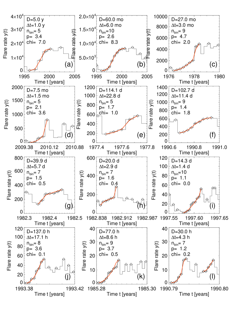
Figure 3: Fitted time profiles $\lambda(t)$ for 12 events with increasing temporal solutions, from $\Delta t=1$ yr (panel a) to $\Delta t=4.3$ hrs (panel l).

We sampled time structures by using an automated detection algorithm, for 12 different time resolutions $\Delta t$, logarithmically spaced with $n_{bin}=2^{i},\ i=0,1,...,12$ per year. The total of detected structures amounts to 848 time structures, ranging from time resolutions of $\Delta t=2$ hrs to $\Delta t=1$ year (Table 1). Each time structure was fitted with the polynomial time profile model $\lambda(t)$ (Eq. 6), and the best-fit three parameters $[t_{0},\lambda_{0},p]$ were determined. We show the detailed fits from a selection of 12 events (out of the 848 detected events) in Fig. 3, selected from 12 different time resolutions and cases with the largest number of time bins (monotonically increasing during the rise time). For instance, the first example shown in Fig. 3a is gathered from $n_{bin}=5$ time bins, a time resolution of $\Delta t$ = (1 year)/$n_{bin}=1.0$ year, a duration of $D=n_{bin}\Delta t=5.0$ years, a nonlinearity index of $p=3.4$, and a goodness-of-fit $\chi=7.0$. Note that the formal error (Eq. 15) is an adequate estimate of the statistical uncertainty in cases with $\chi\lower 1.72218pt\hbox{$\;\buildrel<\over{\scriptstyle\sim}\;$}2$, while high values of $\chi\lower 1.72218pt\hbox{$\;\buildrel>\over{\scriptstyle\sim}\;$}2$ (e.g., Fig. 3a, 3b) indicate under-estimated uncertainties $\chi$ due to very high flare rates (of $\lambda(t_{max})\lower 1.72218pt\hbox{$\;\buildrel>\over{\scriptstyle\sim}\;$}10^{4}$ years^-1) and unknown systematic errors of the model (Eq. 6).

3.3 Measurement of The Nonlinearity Index

The major new result of this analysis is the measurement of the nonlinearity index $p$, which represents the order (or degree) of the polynomial flare rate evolution, $\lambda(t)\propto t^{p}$ (Eq. 6). The physical implication is that we have a diagnostic whether the evolution of an event is linear, $\lambda(t)\propto t$, which is typical for linear random processes, or if the event evolution is nonlinear, $\lambda(t)\propto t^{p}$, which is typical for exponentially growing avalanche processes.

We list the obtained nonlinearity indices $p$ in Table 1, and show their dependence on the time resolution $\Delta t=[1\ year]/n_{bin}$ in Fig. 4. Interestingly, the graph shown in Fig. (4) reveals three different regimes: (i) One group with a cubic nonlinearity of $p=2.83\pm 0.49$ during time ranges from 1.5 months to 1 year, is evidently produced by the solar dynamo, due to the 11-year time scale; (ii) Another group with a quadratic nonlinearity of $p=2.19\pm 0.07$ is found during a time range from 2 hours to 3 days, which is attributed to clustering of solar flares; and (iii) An intermediate group with a nonlinearity of $p=1.83\pm 0.22$ during time ranges from 6 days to 23 days, is most likely affected by the solar rotation rate (which has a sidereal rotation rate of $\approx 26$ days).

A remarkable result is that all fitted nonlinearity indices $p$ yield values in a range of $p\approx$ 1.6-3.5 (Fig. 4). This means that all groups are significantly above the linear (random) range ($p\approx 1$), which suggests that nonlinear physical processes are responsible for all detected time structures, for solar flares, partially occulted long-duration flares, as well as for the solar dynamo. These results on the absence of linear random processes and the ubiquity of nonlinearity ($p\lower 1.72218pt\hbox{$\;\buildrel>\over{\scriptstyle\sim}\;$}2$) demands a theoretical explanation.

4 Discussion

The behavior of the nonlinearity index $p$ gives us some deeper understanding on the waiting time distribution (Section 4.1), the solar rotation effect (Section 4.2), the solar dynamo (Section 4.3), implications for self-organized criticality models (Section 4.4), and the stochasticity, intermittency, and memory of solar flare rates (Section 4.5).

4.1 Waiting Time Distributions

From numerical simulations and analytical calculations of nonstationary waiting time distributions we learned that their power law slope $\alpha$ depends on the nonlinearity index $p$, namely $\alpha=2+1/p$ (Eq. 1), as derived in recent work (Aschwanden, Johnson, and Nurham 2021). Once the nonlinearity index $p$ is known for a given data set, the waiting time distribution $N(\tau)$ is in principle fully determined (with Eqs. 2 or 3), using the analytically derived relationship (Eq. 1). However, the various studies on the waiting time distributions $N(\tau)$ with exact analytical solutions have revealed a high sensitivity on the long waiting times, which corresponds to the time intervals of minimum flare rates and occur at the beginning of exponentially growing flare rates, as modeled with the logistic and polynomial models. It is instructive to study the differences early in flare events (say in the range of $t\lower 1.72218pt\hbox{$\;\buildrel<\over{\scriptstyle\sim}\;$}0.2$ in Fig. 1), which shows relatively large differences of $\approx 2\%$ for a nonlinearity index of $p=2$ (Fig. 1, left), but reveals much smaller differences of $\approx 0.5\%$ for $p=3$ (Fig. 1, right). Thus, this comparison suggests that the logistic approximation is generally more accurate (than the polynomial model) for high nonlinearity indices ($p\lower 1.72218pt\hbox{$\;\buildrel>\over{\scriptstyle\sim}\;$}3$).

A careful analysis of the waiting time distribution for the logistic equation shows that a power law typically only occurs when there is a large increase in rate ($\lambda_{1}/\lambda_{2}\gg 0.1$), and for $1\sim\lambda_{1}\Delta\lower 1.72218pt\hbox{$\;\buildrel<\over{\scriptstyle\sim}\;$}10$. For these parameters, the power law is typically in the range $-2<\alpha<-2.5$ consistent with the power laws obtained from the approximate fit (Eq. 10 with $p\geq 2$) of the solution of the logistic equation.

Here we find different results of the power law slope $\alpha$ among three different groups in Fig. 4, namely for the solar dynamo, solar flare clusters, and partially occulted flares (an effect caused by the solar rotation). In the following we average the power law slopes from 12 different time resolutions. Using the results obtained from the solar dynamo, $p=2.83\pm 0.49$ (Fig. 4), we predict a power law slope of $\alpha=2+1/p\approx 2.4$ (using Eq. 1). For solar flares, with $p=2.19\pm 0.07$ (Fig. 4), we predict a power law slope of $\alpha=2+1/p\approx 2.5$. For the intermediate group, which is affected by the solar rotation with $p=1.83\pm 0.22$ (Fig. 4), we predict a power law slope of $\alpha=2+1/p\approx 2.5$. Thus these three cases cover a range of $\alpha\approx 2.4-2.5$. This result indeed matches closely the power law slopes observed from previous GOES waiting time distributions in the range of $\alpha\approx 2.1-2.4$, reported as $\alpha=2.4\pm 0.1$ (Boffetta et al. 1999), $\alpha=2.16\pm 0.05$ (Wheatland 2000a; Lepreti et al. 2001); $\alpha=2.36\pm 0.11$ (Wheatland and Litvinenko 2002). A similar value of $\alpha=2.5$ was recently calculated for a sinusoidal flare rate function also (Nurhan et al. 2021), instead of the polynomial flare rate model used here.

4.2 Solar Rotation Effect

The temporal variation of the solar flare rate has been studied in terms of the fractal dimension in the case of solar radio emission (Watari 1996a), which led to a diagnostic for periodic, chaotic, and random components (Watari 1996b). A power spectrum $<P(\tau)>$ of the daily sunspot number and radio flux has been calculated, with $\tau$ a time interval, yielding a fractal relationship $<P(\tau)>\propto\tau^{-\alpha}$ and a power law slope in the range of $\alpha\approx 1.2-2.0$. Interestingly they find an effect of the solar rotation, which they simulate with and without the rotational effect. They find a steepening of the power spectrum slope at a time interval of $\tau\lower 1.72218pt\hbox{$\;\buildrel>\over{\scriptstyle\sim}\;$}26$ days.

The manifestation of a solar rotation effect simulated in Watari (1996a, 1996b) affects our data analysis similarly. We carried out some simplified modeling and found that long waiting times are over-represented due to occulting at the solar limb. Solar occulting artificially increases the number of waiting times at $\tau=T_{rot}/2$, as there is an artificial bias that introduces a spurious excess of waiting times at the rotation period.

4.3 The Solar Dynamo

The solar dynamo reverses the solar magnetic field every 11 years, which yields a 22-year cycle for the same magnetic polarity, also called the Hale magnetic cycle. The observational manifestation of this cyclic behavior is also reflected in the decadal variability of the flare rate $\Lambda(t)$ and the power law slope of flare durations (Aschwanden and Freeland 2012), as well as in the variability of the sunspot number (for a recent analysis see Aschwanden and Dudok de Wit 2021). The underlying physical mechanism is a quasi-stationary oscillation of a nonlinear system that is called the limit cycle (for a miniature-review see chapter 3.6 in Aschwanden 2011). It occurs in many nonlinear systems that come close to an oscillatory behavior. Theoretical examples of such nonlinear systems are the Hopf bifurcation (Cameron and Schuessler 2017), or the Lotka-Volterra coupled differential equation system (Consolini et al. 2009) known in ecological sciences (May 1974). The physical mechanism of the solar dynamo cycle can ultimately be understood as a near-equilibrium oscillation between the global solar poloidal magnetic field $B_{r}(t)$ and the toroidal magnetic field $B_{\theta}(t)$ (Charbonneau 2005; Cameron and Schuessler 2017).

Regarding our polynomial approach of characterizing the flare rate variability, $\lambda(r)\propto t^{p}$, the nonlinearity parameter $p$ is an observable, for which values of $p=2.83\pm 0.49$ (Table 1 and Fig. 4) were found. Alternatively, instead of assuming a general polynomial index $p$, a sinusoidal model $\lambda(\tau)\propto 1+\cos(\tau)$ has been used also (Nurhan et al. 2021), yielding a power law-like waiting distribution with a slope of $\alpha=2.5$. Based on the predicted relationship $\alpha=2+1/p$ (Eq. 1) we expect to measure a nonlinearity index of $p=1/(\alpha-2)=2$, which indeed confirms the expected nonlinearity range of $p\lower 1.72218pt\hbox{$\;\buildrel>\over{\scriptstyle\sim}\;$}2$. Some differences could possibly be explained with the asymmetry of the solar cycle time profile $\Lambda(t)$. More specifically, the rise time of a sunspot cycle varies inversely with the cycle amplitude: Strong cycles rise to their maximum faster than weak cycles, also known as Waldmeier effect.

4.4 Self-Organized Criticality Models

The most conspicuous feature of self-organized criticality (SOC) models is the avalanche behavior of events in a nonlinear dissipative system, leading to power law slopes of their size distribution and their duration distribution (Bak et al. 1987; 1988). The simplest dynamic model of a SOC avalanche can be described by an (initial) exponential growth phase after the onset of an instability, and saturation of the instability after a random time. These two assumptions directly predict a power law-like distribution of avalanche sizes. Besides this exponential-growth model (Willis and Yule 1922; Rosner and Vaiana 1978; Aschwanden 1998), a power law-growth model (which is equivalent to our polynomial time evolution), and a logistic-growth model have also been formulated (Aschwanden 2011). (e.g., May 1974; Beltrami 1987, Jackson 1989, Aschwanden 2011, p.94),

If we interpret time structures with a nonlinearity index $p$ as SOC avalanches, we need to test whether a polynomial event rate model $\lambda(t)\propto t^{p}$ is consistent with a logistic model. Such a comparison is shown in Fig. 1, where the two functions are almost indistinguishable. Consequently, we can use the logistic model and the polynomial model equally well as a discriminative diagnostic between linear ($p\approx 1$) and nonlinear ($p\lower 1.72218pt\hbox{$\;\buildrel>\over{\scriptstyle\sim}\;$}2$) systems. This has far-reaching consequences for SOC models. Traditional SOC models assume a slow-driven and stationary flaring rate (Bak et al. 1987, 1988), while more recent studies adjust to (i) multiple energy dissipation episodes during individual flares, (ii) violation of time scale separation (between flare durations and waiting times), and (iii) fast-driven and nonstationary flaring rates (Aschwanden 2019b).

4.5 Stochasticity and Memory

There are at least three unmistakable dynamic patterns of dissipative systems: linear, non-linear, and limit-cycle systems.

The first mechanism is a linear system, where the total dissipated energy grows linearly with the energy input, the energy dissipation rate or event rate is constant, and the resulting waiting time distribution is exponentially dropping off, $N(\tau)\propto\exp{[-\tau]}$, according to a random process. As an example we consider the accumulated number of photons emitted from the Sun or a star in a fixed distance. Such a random process has no memory by definition, which implies that random fluctuations are uncorrelated and incoherent in a time profile. Earlier studies suspected that energy storage in solar flares accumulates as a linear function of time, which implies a correlation between the waiting time and the energy released during two subsequent flares (Rosner and Vaiana 1978), but such a predicted correlation was never found (Lu 1995; Crosby 1996; Wheatland 2000b; Georgoulis et al. 2001).

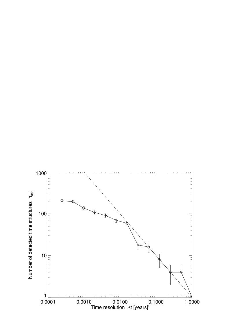
Figure 5: The number of detected time structures $n_{det}$ as a function of the time resolution (thick linestyle with error bars) and predicted upper limit (dashed linestyle).

A second mechanism is a nonlinear system, where the total dissipated energy grows nonlinearly, the energy dissipation rate or event rate is not constant, and the resulting waiting time distribution is close to a power law distribution, $N(\tau)\propto\tau^{-\alpha}$. The time evolution of an exponentially growing system is produced by a coherent amplification mechanism, triggered by an instability of a system. In the parlance of self-organized criticality systems, an avalanche takes place that grows coherently over the duration of an event. This could be a magnetic reconnection process that is very common in solar and stellar flare physics. The coherence of an exponentially growing system implies that there is a memory effect over the duration of an event. The basic behavior of an avalanching system in terms of next-neighbor interactions in a lattice grid has been simulated extensively (Bak et al. 1987, 1988; Pruessner 2012). The critical diagnostic of coherent versus incoherent growth is quantified here with a nonlinearity index $p$, from which we can obtain information on what time scales a nonlinear system has memory, and whether observed fluctuations are due to random noise or coherent time structures with memory. It appears that the solar flare rate exhibits memory from time scales of hours (during clustered flares in an unstable active retion) to decades, driven by the magnetic (Hale) solar cycle. The number of (coherent) detected time structures as a function of the time resolution is shown in Fig. 5, which obeys the upper limit $n_{det}\leq$ (1 year)/$n_{bin}$ (Fig. 5, dashed linestyle).

A third mechanism is the limit-cycle behavior of a coupled nonlinear system, which exhibits an oscillary pattern. An example is the solar cycle, which oscillates between a poloidal and a toroidal global magnetic field. The oscillatory behavior is often accomplished by a driving force and a feedback force that balance each other in a quasi-equilibrium phase space, although the two counteracting forces are delayed to each other by about a half period. There exist also linearly (strictly periodic) oscillating mechanisms (e.g., pendulum, planetary resonances, coronal loop kink-mode oscillations), in contrast to the less regular nonlinear mechanisms. Since oscillations occur over durations much longer than a single period, we can attribute a memory time scale at least over the duration of the observation, or during a time interval with a constant oscillation period. In other words, the oscillation period is the memorized piece of information.

5 Conclusions

We analyze the waiting times in the largest data sets of solar flare events, obtained from GOES soft X-ray light curves, by using variable time resolutions from 2 days to 4 decades. The automated flare detection algorithm gathers over $3\times 10^{5}$ events, from which we identify $\approx 10^{3}$ events with significant coherent growth characteristics. We define the nonlinear growth phase (rise time) in terms of a polynomial (as well as logistic) time evolution, which allows us to discriminate linear random events ($p\approx 1$) from nonlinear energy dissipation events ($p\lower 1.72218pt\hbox{$\;\buildrel>\over{\scriptstyle\sim}\;$}2$). The memory time of the Sun is essentially defined by time structures with coherent growth, such as exponential-growing solar flare clusters. We obtain the following results:

1. On time resolutions of $T\approx$ 1.5 months to 1 year, the most prevailing nonlinear time structure is the solar dynamo, which can be considered as a nonlinear system with limit-cycle behavior, with an average period of 11 years. The degree of nonlinearity is found to be $p=2.8\pm 0.5$, averaged over four solar cycles and various time resolutions. The corresponding power law slope is predicted to be $\alpha=2+1/p\approx 2.4$, which is close to the value $(\alpha=2.5)$ calculated for a sinusoidally oscillating flare rate (Nurhan et al. 2021). The sinusoidal flare rate variability can be understood by the oscillatory solar dynamo, where the poloidal and the toroidal magnetic field vary sinusoidally in anti-phase.

2. Solar flares are found not to occur in random order, although the flare rate time profile appears to consist of many randomly scattered fluctuations of the flare rate. Instead, clusters of flares are found at time resolutions from 2 hours to 3 days, which represents some memory over these time scales. It indicates that coherent growth in the flare rate is nearly quadratic, with a mean nonlinearity index of $p=2.2\pm 0.1$.

3. At intermediate time resolutions from 6 days to 23 days, the solar rotation occults some flare clusters partially, causing a lower but still significant nonlinearity index of $p=1.8\pm 0.2$.

4. The determination of the nonlinearity index $p$ allows us to predict the power law slope $\alpha$ of the waiting time distribution, $\alpha=2.0+1/p$, predicting values in the range of $\alpha=2.4-2.5$, which agrees with the observational values of $\alpha=2.1-2.4$.

5. The nonlinearity index range of $p\lower 1.72218pt\hbox{$\;\buildrel>\over{\scriptstyle\sim}\;$}2$ is consistent with the exponentially-growing characteristic of avalanches governed by self-organizing criticality.

The main new result of this study is the demonstration that the Sun reveals memory over a huge range of time scales, from a few hours to several decades, rather than producing flares in random order. This means that nonlinear physical processes produce spatio-temporal structures with coherent time evolutions, such as instabilities with exponential growth and subsequent decay. There are self-organized avalanche processes with clustered (sympathetic) flare generation, which occurs at a higher hierarchical level than the avalanches of individual flare events.

Acknowledgements: Part of the work was supported by NASA contracts NNG04EA00C and NNG09FA40C. JRJ acknowledges NASA grant NNX16AQ87G.

References

Aschwanden, M.J., Dennis, B.R., and Benz, A.O. 1998, ApJ 497, 972

Aschwanden, M.J. and McTiernan, J.M. 2010, ApJ 717, 683

Aschwanden, M.J. 2011 Self-Organized Criticality in Astrophysics. The Statistics of Nonlinear Processes in the Universe, Springer-Praxis: New York, 416p.

Aschwanden, M.J. 2012a, AA 539:A2

Aschwanden, M.J. 2012b, ApJ 757, 94

Aschwanden, M.J. and Freeland, S.M. 2012, ApJ 754:112

Aschwanden, M.J., Crosby, N., Dimitropoulouy, M., et al. 2016, SSRv 198:47

Aschwanden, M.J. 2019a, ApJ 880, 105

Aschwanden, M.J. 2019b, ApJ 887:57

Aschwanden, M.J. and Dudok de Wit, T. 2021, ApJ 912:94

Aschwanden, M.J., Johnson, J.R., and Nurhan, Y.I., 2021, GRL (subm.)

Bak, P., Tang, C., and Wiesenfeld, K. 1987, Physical Review Lett. 59/27, 381

Bak, P., Tang, C., and Wiesenfeld, K. 1988, Physical Rev. A 38/1, 364

Bauke, H. 2007, Eur.Phys.J.B. 58, 167

Beltrami, E. 1987, Mathematics for dynamic modeling, Academic Press, Inc: Boston

Boffetta, G., Carbone, V., Giuliani, P., Veltri, P., and Vulpiani, A. 1999, Phys.Rev.Lett. 83, 4662

Bourouaine, S., Perez, J.C., Klein, K.C., Chen, C.H.K. 2020, ApJ 904, 308

Cameron, R. and Schuessler, M. 2017, ApJ 843, 111

Charbonneau, P. 2005, Living Reviews in Solar Physics 2, 2

Consolini, G., Tozzi, R., and De Michelis P. 2009, A&A 506, 1381

Crosby, N.B. 1996, PhD Thesis, University Paris VII, Meudon, Paris, 348p.

Dudok de Wit, P., Krasnoselskikh, V.V., Bale, S.D., et al. 2020, ApJSS 246:39

Eastwood, J.P., Wheatland, M.S., Hudson, H.S., et al. 2010, ApJ 708, L95

Greco, A., Matthaeus, W.H., Servidio, S., Chuychai, P. and Dmitruk, P. 2009, ApJ 2, L111

Georgoulis,M.K., Vilmer,N., and Croby,N.B. 2001, AA 367, 326

Goldstein, M.L., Morris, S.A., and Yen, G.G. 2004, Eur.Phys.J.B. 41, 255

Gorobets, A. and Messerotti, M. 2012, SoPh 281, 651

Grigolini, P., Leddon,D., and Scafetta,N. 2002, Phys.Rev.Lett E, 65/4. id. 046203

Guidorzi,C., Dichiara, S., Frontera,F., et al. 2015, ApJ 801, 57

Hawley, S.L., Davenport, J.R.A., Kowalski, A.F., Wisniewski, John P. et al. 2014, ApJ 797, 12H

Hudson, H.S. 2020, MNRAS 491, 4435

Jackson, E.A. 1989, Perspectives of nonlinear dynamics (Lotka-Volterra equation, p.283), Cambridge University Press: Cambridge

Leddon, D. 2001, eprint arXiv:cond-mat/0108062, Dissertation Abstracts International, Volume: 63-12, Section: B, page: 5891; 56 p.

Lepreti, F., Carbone, V., and Veltri,P. 2001, ApJ 555, L133

Li, C., Zhong, S.J., Wang, L., et al. 2014, ApJ 792, L26

Li, C., Zhong, S.J., Xu, Z.G., et al. 2018, MNRAS 479 L139

Lu, E.T. 1995, ApJ 447, 416

May, R.M. 1974, Model Ecosystems, Princeton

Morales, L.F. and Santos, N.A. 2020, SoPh 295, 155

Norman, J.P., Charbonneau, P., McIntosh, S.W., and Liu, H. 2001, ApJ 557, 891

Nurhan, Y.I., Johnson, J.R., Homan, R., et al. (2021), GRL, (subm.)

Newman, M.E.J. 2005, Contemp.Phys. 46, 323

Pruessner, G. 2012, Self-organised criticality. Theory, models and characterisation, Cambridge University Press: Cambridge

Qin, G. and Wu, S.S. 2018, ApJ 869, 48

Rosner,R., and Vaiana,G.S. 1978, ApJ 222, 1104

Usoskin, I.G., Solanki, S.K., and Kovaltsov, G.A. 2017, AA 471, 301

Wang, F.Y., Dai, Z.G., Yi, S.X., and Xi, S.Q. 2015, ApJS 216, 8

Wang, H.N., Cui, Y.M., and He,H. 2009, Res.Astron.Astrophys. 9, 687

Wang, J.S., Wang, F.Y., and Dai, Z.G. 2017, MNRAS 471 2517

Wang, Y., Liu, L., Shen, C., et al. 2013, ApJ 763, L43

Wanliss, J.A. and Eygand, J.M. 2007, GRL 34, 4107

Watari, S. 1996a, Solar Phys 163, 371

Watari, S. 1996b, Solar Phys 168, 413

Wheatland, M.S., Sturrock,P.A., and McTiernan,J.M. 1998, ApJ 509, 448

Wheatland,M.S. 2000a, ApJ 536, L109

Wheatland,M.S. 2000b, SoPh 191, 381

Wheatland,M.S. 2000c, ApJ 532, 1209

Wheatland, M.S. and Litvinenko, Y.E. 2002, SoPh 211, 255

Wheatland, M.S. 2003, SoPh 214, 361

Wheatland, M.S., and Craig, I.J.D. 2006, SoPh 238, 73

Willis, J.C. and Yule, G.U. 1922, Nature 109, 177

Yeh, C.T., Ding, M., and Chen, P. 2005, ChJAA 5, 193

Yi, S.X., Xi, S.Q., Yu, Hai et al. 2016, ApJS 224, 20

Table 1: Nonlinearity index $p(\Delta t)$ of flare rate function $y(t)$ as a function of the time resolution $\Delta t$.

Time	Number of	Number of	Nonlinearity	Nonlinearity	Nonlinear
resolution	time bins	events	index	median	system
$\Delta t$	$n_{bin}/yr$	$n_{ev}$	$p$	$p_{med}$
1 yr	1	1	3.51$\pm$0.08	3.51	solar dynamo
6 months	2	4	2.54$\pm$0.26	0.26	solar dynamo
3 months	4	4	2.83$\pm$1.70	2.79	solar dynamo
1.5 month	8	8	2.43$\pm$1.76	1.91	solar dynamo
23 days	16	16	1.63$\pm$1.40	1.18	solar rotation
11 days	32	18	1.81$\pm$1.54	1.47	solar rotation
6 days	64	59	2.06$\pm$1.78	1.42	solar rotation
3 days	128	70	2.25$\pm$1.91	1.63	solar flares
1.4 days	256	91	2.12$\pm$1.61	1.45	solar flares
17 hours	512	108	2.15$\pm$1.83	1.57	solar flares
8 hours	1024	137	2.23$\pm$1.55	1.88	solar flares
4 hours	2048	195	2.11$\pm$1.22	1.84	solar flares
2 hours	4096	206	2.29$\pm$1.37	2.11	solar flares

Figure 4: The nonlinearity index $p(\Delta t)$ as a function of the time resolution $\Delta t$ is calculated from an automated GOES flare detection algorithm. Note the triple regimes of solar flares (in the time range of $\Delta t\approx$ 2 hrs - 3 days), the solar rotation (in the time range of $\Delta t\approx$ 6 - 45 days), and the solar dynamo (in the time range of $\Delta t\approx$ 1.5 months - 1 year).