Quantum Molecular Unfolding

Abstract

Molecular Docking (MD) is an important step of the drug discovery process which aims at calculating the preferred position and shape of one molecule to a second when they are bound to each other. During such analysis, 3D representations of molecules are manipulated according to their degree of freedoms: rigid roto-translation and fragment rotations along the rotatable bonds. In our work, we focused on one specific phase of the molecular docking procedure i.e. Molecular Unfolding (MU), which is used to remove the initial bias of a molecule by expanding it to an unfolded shape. The objective of the MU problem is to find the configuration that maximizes the molecular area, or equivalently, that maximizes the internal distances between atoms inside the molecule. We propose a quantum annealing approach to MU by formulating it as a High-order Unconstrained Binary Optimization (HUBO) which was possible to solve on the latest D-Wave annealing hardware (2000Q and Advantage). Results and performances obtained with quantum annealers are compared with state of art classical solvers.

Introduction

Drug Discovery Lyne (2002) is a process that includes several phases, from virtual in silico simulations to in-vitro and in-vivo experimentation. Molecular Docking Meng et al. (2011) (MD) is an important step of the drug discovery process which aims at calculating the preferred position and shape of one molecule to a second when they are bound to each other. The computational resources needed to address MD related tasks are usually quite large, as problems of this kind involve several degrees of freedom and rapidly growing dimensionality.

In recent years, the field of Quantum Computing Nielsen and Chuang (2010) (QC) has undergone significant developments from both hardware and algorithms points of view. In particular, we are living in the so-called NISQ Preskill (2018) era in which it is not clear whether the quantum devices currently available are actually capable of producing better or comparable results compared to classical methods.

In this work, we explored the possibility of using a QC technique called Quantum Annealing McGeoch (2014); Babej et al. (2018); Marchand et al. (2019) (QA) in the virtual screening phase of MD. In particular, we focused on the Molecular Unfolding (MU) process, which is the first step in geometric molecular docking techniques. MU aims at finding the molecular configuration that maximizes its volume, or equivalently, that maximizes the internal distances between atoms inside the molecule.

Our aim was to develop a Quantum Molecular Unfolding approach and execute it on the latest quantum annealing hardware (D-Wave Advantage and 2000Q) in order to understand the capabilities of these devices and compare their performances to state-of-art molecular docking methods.

The remainder of the paper is structured as follows. In the first section, the topic of molecular docking is introduced, followed by a section where the problem of Molecular Unfolding is discussed. In Sec.3, concepts of quantum annealing are illustrated while in Sec.4 a binary optimization formulation of the problem is given. Later in the fifth section, the dataset and pre-processing steps employed before the unfolding phase are presented. This is followed in Sec.6 by a review of state of the art classical algorithms employed to compare solutions obtained with the quantum devices. Finally, in the last two sections, results regrading the embedding on the QPUs are presented as well as a detailed performance comparison between the different methods.

I Preliminaries on Molecular Docking

In-silico approach to drug discovery Lyne (2002) can be viewed as a multi-tiered process that encompasses several sequential computational techniques with the aim of screening virtual libraries of the order of billions of compounds for the most suitable molecules to forward to later experiments.

Molecular Docking Meng et al. (2011) (MD) is an essential step in virtual screening which is used to simulate the atomic interactions of a ligand inside a protein binding site, in order to highlight their possible biochemical reactions and predict whether a stable complex could be formed.

Figure 1: Visual representation of Molecular Docking for a ligand inside a protein pocket, similar to the relation between locks and keys.

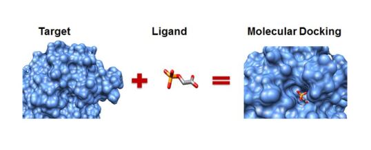
The MD process is divided in two main tasks:

• Detection of three-dimensional poses of the ligand, i.e. valid ligand conformations, positions and orientations inside the active site of the protein (usually called pocket).

• Ranking of the poses via a scoring function. Usually the lower the docking score, the better the resulting binding affinity.

Since electrons inside atoms are repulsive to each other, their interaction affects both molecular shape and reactivity. Therefore, by controlling the molecular shape, it is possible to predict the ligand reactivity to a protein’s pocket as well as the energy cost of such configuration. This direct connection between molecular conformation and binding affinity is what enables geometrical scoring functions Gadioli et al. (2020).

In our approach, the docking process considers the pocket as a rigid structure, while the ligand is a flexible set of atoms. Furthermore, from a strictly geometrical interpretation, the ligand can be seen as a set of chemical bonds (or edges) with a fixed length, where only a subset of edges are rotatable.

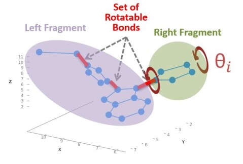
Rotatable bonds (or torsionals) are bonds that split the molecule in two nonempty disjointed fragments, when virtually removed. Consequently, such fragments can rotate independently from each other around the axis of the rotatable bond. These concepts are graphically reported in Fig.2, where the rightmost rotatable bond is splitting the molecule in left and right fragment. Finally, note that the number of fragments in a molecule is usually double the number of rotatables.

Figure 2: Fragments and rotatable bonds

In general, it is possible to point out three main phases in MD: Ligand expansion, Intial Placement and Shape Refinement inside the pocket.

Here we focus on the ligand expansion phase, which is essential for improving docking. In fact, an initial pose of the ligand that is set a priori may introduce shape bias affecting the final quality of the docking. Molecular Unfolding (MU) is the technique used for removing such initial bias by expanding the ligand to an unfolded shape.

II Molecular Unfolding Problem Definition

The objective of the MU problem is to find the unfolded shape of the ligand or, in other terms, the torsion configuration that maximises the molecular volume expressed as total sum of internal distances between pairs of atoms in the ligand. The starting point is the folded molecule defined by a set of atoms together with its fixed and rotatable bonds. We can assign to each rotatable bonds $t_{i}$ a variable corresponding to the angle $\theta_{i}$ which is responsible for fragment rotation. As a convention, we identify the ordered set of rotations by a vector:

$$t=\begin{bmatrix}\theta_{1},\theta_{2},\ldots,\theta_{n}\end{bmatrix}$$ (1)

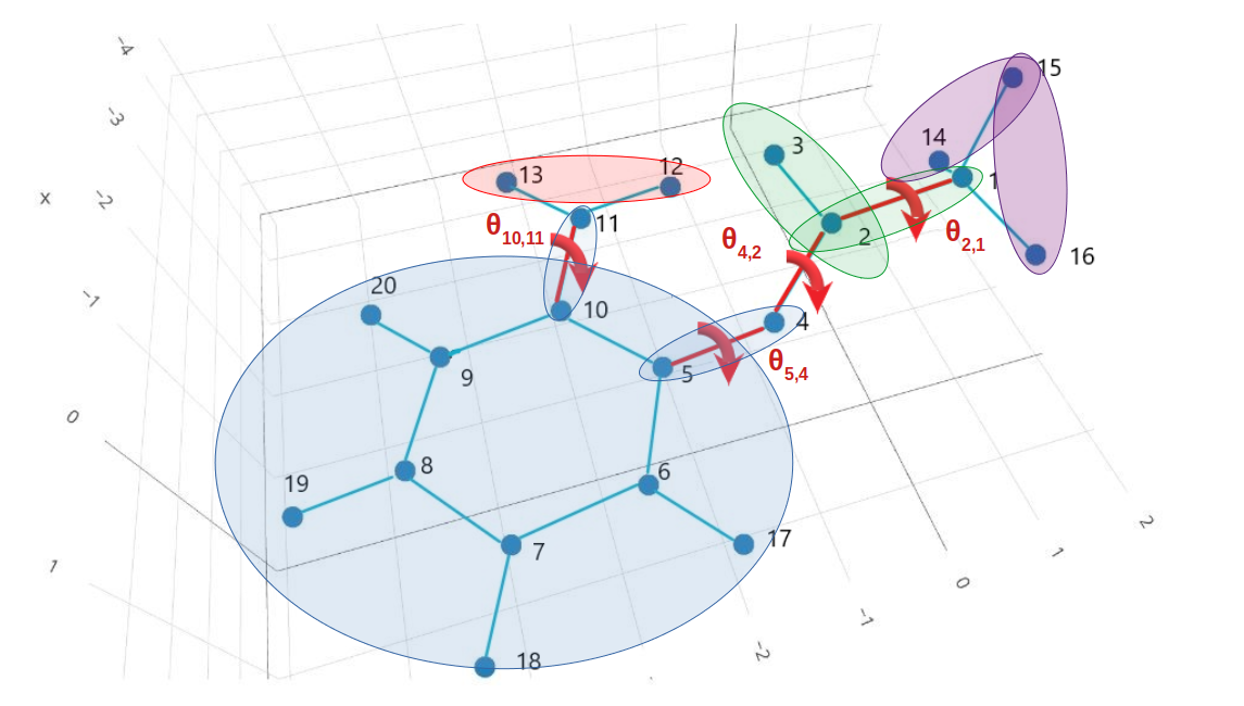
where each torsion $\theta_{i}$ around the bond’s axis can assume values $\left[0,2\pi\right)$. Given a molecule, it is possible to construct the associated graph as shown in Figure 3 where edges represent bonds (which can not contract). Torsional bonds are depicted in red in the image below.

Figure 3: Illustration of a simple organic molecule. The molecular structure presents 4 rotatable bonds, highlighted in red in the graph representation.

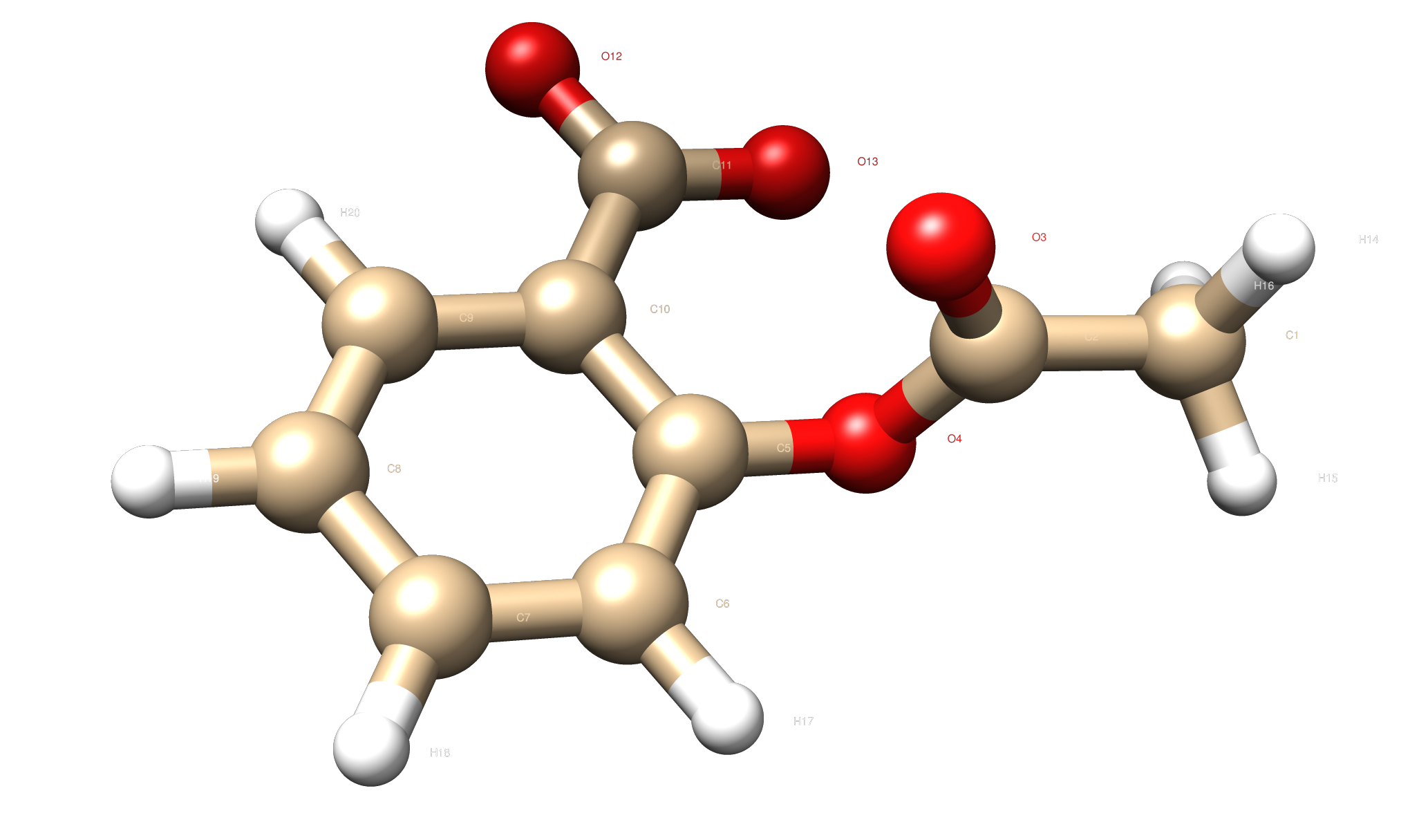
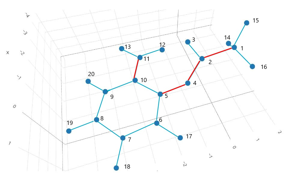
The objective for the MU problem can be expressed in mathematical terms as follows: given a molecule, find the torsional configuration

$$\centering\boldsymbol{\mathbf{t^{unfold}}}=[\theta_{1}^{unfold},\,\dots,\theta_{M}^{unfold}]\@add@centering$$ (2)

such that the following quantity is maximised

$$\centering D({\bf\boldsymbol{\mathbf{t}}})=\sum_{\begin{subarray}{c}a,b\in\mathcal{M}\\ a\neq b\end{subarray}}D_{ab}({\Theta})^{2}\,\@add@centering$$ (3)

The function $D_{ab}(\Theta)$ denotes the distance between two different atoms $a$ and $b$ belonging to the molecule $\mathcal{M}$ while $D(\bf{\boldsymbol{\mathbf{t}}})$ is the sum of all square distances between atoms.

The rationale behind this choice is that the objective function is simple and relies just on the geometry of the molecule. Each distance $D_{ab}(\Theta)$ only depends on the angles induced by those rotatable bonds that appear in the shortest path connecting atom $a$ to $b$ in the graph.

It is worth noticing that it is not necessary to calculate all the pairwise distances that are expressed in equation 3. In fact, it is possible to apply simplifications to $D_{ab}(\Theta)$, as expressed by the following two conditions:

1. The shortest path between two atoms must contain at least one torsional. This is due to the fact that if two atoms belong to the same rigid fragment, their relative position never changes.

2. The shortest path connecting two atoms must have at least three edges. This is a consequence of the fact that atoms connected by only one or two bonds have always the same distance, even when bonds are rotated.

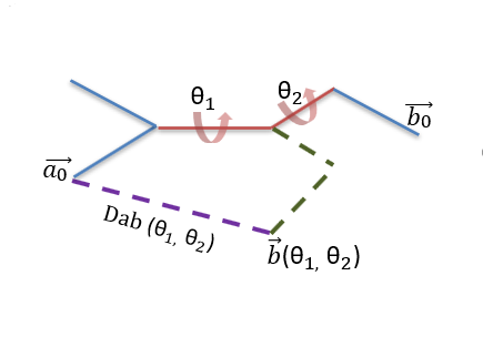
A useful mathematical representation for rotations are rotation matrices, $R(\theta_{i})$, which are function of the angle $\theta_{i}$ associated to torsion $T_{i}$ . If two atoms are connected via multiple torsional, the rotation matrix $R({\Theta})=R(\theta_{i},\theta_{j},\dots,\theta_{k})$, characterizing their relationship is an ordered multiplication of single torsion rotation matrices

$$R({\Theta})=R(\theta_{i},\theta_{j},\dots,\theta_{k})=R(\theta_{i})\times R(\theta_{j})\times...\times R(\theta_{k})$$ (4)

Each rotation $R(\theta_{i})$ is expressed via a $4\times 4$ rotation matrix acting on atomic coordinates. The extremes of a bond connecting two atoms are identified by the coordinates of the atoms themselves.

Consider now the distance $D_{ab}({\Theta})$ and the initial positions of atoms $a$ and $b$ which are identified with $\vec{a_{0}}$ and $\vec{b_{0}}$ respectively. Relative positions are obtained by fixing one of the two atoms while rotating the other as follows

$$\vec{a}=\vec{a_{0}}\ \,\ \ \ \ \ \ \vec{b}=R({\Theta})\vec{b_{0}}$$ (5)

Hence, we can rewrite the single contributes in equation 3 using the Euclidean distance as

$$D_{ab}({\Theta})^{2}=\|\vec{a_{0}}-R({\Theta})\vec{b_{0}}\|^{2}$$ (6)

Figure 4 shows how the relative positions change as function of the angles assumed by the two rotatable bonds.

Figure 4: Visual representation of the action of two rotations $\theta_{1}$ and $\theta_{2}$ on the distance expressed in eq. 6.

III Quantum Annealing

Quantum annealing (QA) is a meta-heuristic technique for addressing challenging combinatorial problems. It can be seen as a variation of the Simulated Annealing (SA) Kirkpatrick et al. (1983) algorithm where quantum fluctuation, instead of thermal effects, are employed in the exploration of the configuration space. Quantum annealing devices, like those implemented with superconductive qubits by the Canadian company D-Wave, are able to solve combinatorial problems expressed in Quadratic Unconstrained Binary Optimization (QUBO) terms. A generic QUBO problem is defined as

$$O(x)=\sum_{i}h_{i}{x}_{i}+\sum_{i>j}J_{i,j}x_{i}x_{j}$$ (7)

where $x_{i}\in\left\{0,1\right\}$ are binary variables while $h_{i}$ and $J_{ij}$ are parameters whose values encode the optimization task in such a way that the minimum of $O(x)$ represents the solution to the optimization problem.

In general, a given optimization problem can be easily translated in binary combinatorial terms as a a high-order quadratic unconstrained binary optimization (HUBO) problem.

$$O_{Hubo}(x)=\sum_{i}\alpha_{i}{x}_{i}+\sum_{i,j}\beta_{i,j}x_{i}x_{j}+\sum_{i,j,k}\gamma_{i,j,k}x_{i}x_{j}x_{k}+...$$ (8)

Fortunately, it is always possible to convert HUBOs into QUBOs. The trick used is to add new ancillary binary variables and substitute high-order terms with sums of quadratic expressions (made up with original binary variables and new ones) in order to preserve local and global minima Mengoni et al. (2020).

As an example, a cubic term like $\pm x_{1}\cdot x_{2}\cdot x_{3}$ can be divided using the ancillary binary variable $a_{1}$ as

$$\pm x_{1}\cdot x_{2}\cdot x_{3}\rightarrow\pm a_{1}x_{3}+2(x_{1}x_{2}-2x_{1}a_{1}-2x_{2}a_{1}+3a_{1})$$ (9)

I practice, one can decide to build a custom function for quadratisation or exploit the functions present in D-Wave software offer such as make_quadratic.

IV HUBO Formulation

As a first step, it is necessary to formulate the MU problem in binary optimization terms in order to employ a quantum annealing approach.

Let us consider a discretisation of the angle $\theta_{i}$ associated to a rotatable bond $T_{i}$ into $d$ possible values

$$\theta_{i}=[\theta_{i}^{1},\theta_{i}^{2},\theta_{i}^{3},...,\theta_{i}^{d}]$$ (10)

As a consequence, continuous functions of the angles like sine and cosine can be discretised as well in $d$ values

$$\sin(\theta_{i}) =[\sin(\theta_{i}^{1}),\sin(\theta_{i}^{2}),\sin(\theta_{i}^{3}),...,\sin(\theta_{i}^{d})]$$ (11)

$$\cos(\theta_{i}) =[\cos(\theta_{i}^{1}),\cos(\theta_{i}^{2}),\cos(\theta_{i}^{3}),...,\cos(\theta_{i}^{d})]$$ (12)

Moreover, since torsional angles can assume only one value at a time, it is necessary to associate each $\theta_{i}$ with only one value among all the possible $\theta_{i}^{k}$. A One-Hot Encoding strategy is adopted for each torsional $T_{i}$, to which are assigned binary variables $x_{ik}$, with $1\leq k\leq d$, such that

$$x_{ik}=\begin{cases}1&\text{if }\theta_{i}=\theta_{i}^{k};\\ 0&\text{otherwise.}\end{cases}$$ (13)

Definition 13 tells us that only one among the binary variables can be assigned to a one or truth value. This means that their sum is always equal to one:

$$\sum_{k=1}^{d}x_{ik}=1$$ (14)

Note that equation 14 must hold for all rotatables. In order to convert such algebraic constraint into QUBO, the following term has to be considered:

$$\sum_{i}\left(\sum_{k=1}^{d}x_{ik}-1\right)^{2}$$ (15)

Constraint of eq. 15 is usually called a hard constraint because it is mandatory to satisfy this term i.e. minimize it in the combinatorial optimization.

Regarding those functions that appear in the rotation matrix $R({\theta_{i}})$ such as $\sin(\theta_{i})$ and $\cos(\theta_{i})$, they can be expressed as

$$\sin(\theta_{i}) =\sum_{k=1}^{d}\sin(\theta_{i}^{k})\ x_{ik}$$ (16)

$$\cos(\theta_{i}) =\sum_{k=1}^{d}\cos(\theta_{i}^{k})\ x_{ik}$$ (17)

Therefore, a rotation matrix $R({\theta_{i}})$ becomes a function of all the binary variables $x_{ik}$ needed to represent the angle $\theta_{i}$

$$R({\theta_{i}})=R(x_{i1},x_{i2},...,x_{id})$$ (18)

For a generic rotation we have

$$R({\Theta}) =R(\theta_{i})\times R(\theta_{j})\times...\times R(\theta_{k})$$

$$=R(x_{i1},x_{i2},...,x_{id})\times R(x_{j1},x_{j2},...,x_{jd})\times...$$

$$...\times R(x_{k1},x_{k2},...,x_{kd})$$ (19)

Note that, for what concerns the granularity of the rotations, in order to obtain a precision of $\Delta\theta_{i}=~{}\theta_{i}^{k+1}-~{}\theta_{i}^{k}$ in the representation of angle $\theta_{i}$, the number of variables $x_{ik}$ needed for each torsion is given by

$$d=\dfrac{2\pi}{\Delta\theta_{i}}=\dfrac{2\pi}{\theta_{i}^{k+1}-\theta_{i}^{k}}$$ (20)

Given a number $M$ of torsional bonds, the total number of binary variables is

$$n=d\times M=\dfrac{2\pi}{\Delta\theta_{i}}\times M$$ (21)

The general form of the HUBO optimization function can be written as

$$O(x_{ik})=A_{const}\sum_{i}\left(\sum_{k=1}^{d}x_{ik}-1\right)^{2}-\sum_{\begin{subarray}{c}a,b\end{subarray}}D_{ab}({\Theta})^{2}$$ (22)

In the last equation, the second term identifies the optimization term, which has a minus sign in front because it should be maximized (while the whole expression is minimized). The first term instead represent the hard constraint, where the parameter $A_{const}$ is a penalty scalar that modulates its strength. Finally, it is worth noticing that, given a molecule with $M$ torsionals, the highest order term appearing in eq.22 is $2M$, where the number 2 comes from the squared distances.

V Dataset and Pre-processing

V.1 Ligand Dataset

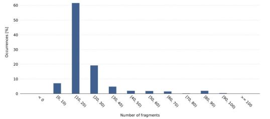
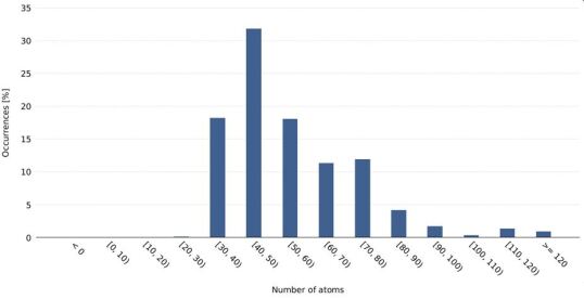
The original ligand dataset in our possession is made up of 118 molecules, with a number of atoms ranging form 20 to more that 120 and a number of torsionals going from few units to about 50.

As shown in Figure 5 below, it is possible to see that 60% of the ligands in our database present 10-20 fragments, which means 5-10 rotatable bonds. The number of atoms is peaked about the 40-50 interval. For this reason, we decided to concentrate our research only on molecules that had at most $12$ rotatable bonds and an increasing number of atoms going from $20$ to $50$.

Since our study aimed at highlighting the change in problem complexity by increasing the number of torsionals, we considered only a subset of torsionals at a time, out of 12 possible rotatable bonds.

Figure 5: Analysis of the distribution for number of atoms and number of fragments.

V.2 Pre-processing Phase

The pre-processing starts with the parsing of the information about the molecule via analysis of its .MOL2 file. A graph containing a three-dimensional description of the ligand together with bond type (bonds could be single, double, triple, amide or aromatic) is constructed.

Two simplifications related to chemical-physical properties of ligands are applied in the pre-processing phase: one is due to the fact that only single and aromatic bonds can be rotatable, while the other concerns the removal of terminal hydrogen atoms whose distances with the rest do not affect the total sum of internal distances. Note that the removal of terminal hydrogens may trigger the generation of conformations where the final position of atoms do not satisfy their minimum Van Der Waals distance. Such invalid shapes are discarded in post-processing.

After this, the graph associated to the molucle is divided into fragments as shown in Figure 6. At this stage, the betweenness centrality Freeman (1977), defined in equation 23, is employed to obtain an ordering of the atoms within the graph. By consequence, this procedure also specifies an ordering of rotatable bonds.

$$\mathrm{Betweeness\ centrality\ of\ atom\ \textit{v}\mathrel{\mathop{\mathchar 58\relax}}}\ \ \sum_{v\neq s\neq t}\frac{\sigma_{st}(v)}{\sigma_{st}}$$ (23)

Equation 23 is calculated for each atom $v$ as the sum of all the possible shortest paths connecting atoms $s$ and $t$ which also cross $v$, divided by the total number of shortest paths between $s$ and $t$. The atom with the greatest centrality is chosen as centre of the graph and origin of the torsional ordering.

Each fragment is identified as a set of atoms influenced by the same set of rotatable bonds, called rotatables influence set. The definition of rotatables influence set is the following

$$\mathrm{Rotables\ influece\ set\ \mathrel{\mathop{\mathchar 58\relax}}\ }\ \ I_{s}=E_{C_{a,a_{k}}}\cap E_{R}$$ (24)

$C_{a}$ = atom with greatest betweeness centrality
$E_{R}$ = Rotatable bonds 
$E_{C_{a},a_{k}}$ = Bonds on the shortest path $\sigma_{C_{a},a_{k}}$

Atoms of the same fragment are mapped to a unique shortest path, which is composed by a set of edges belonging to the influence set.

Figure 6: Atoms belonging to the same fragment, depicted using colors, are affected by the same rotatables influence set.

Finally, contributions appearing in equation 6 are obtained for each fragment, where distances between atoms are calculated only once and respecting conditions 1 and 2. Distances between atoms belonging to the same fragment are fixed, hence not considered.

VI Model Development

VI.1 Distance Simplification

The first simplification concerns the calculation of contributions in equation 6, as the number of terms increases quadratically with the number of atoms involved. Hence, instead of measuring the Euclidean distance between each atom $a$ in fragment $A$ and each atom $b$ in fragment $B$, only distances between different fragments have been considered. In particular, each fragment was identified with the coordinates of the median atom inside the fragment.

Partial contributions for single fragments are summed up together in the HUBO as in equation 22. Note that such optimization function is a non-linear symbolic expression where symbolic variables representing torsional angles appear in the rotation matrix in the form of trigonometric functions as defined in equation 16.

VI.2 Coarse-grained Rotations

The number of variables needed to express the MU problem in combinatorial optimization form depends on the discretisation of the angles, as shown in eq. 20. It is therefore essential to understand how to chose an optimal granularity for the torsionals. In this regard, previous knowledge about the dataset was used to obtain approximate solutions achieving an acceptable quality.

Figure 7: Analysis of the degradation by transitioning to a coarse-grained rotation.

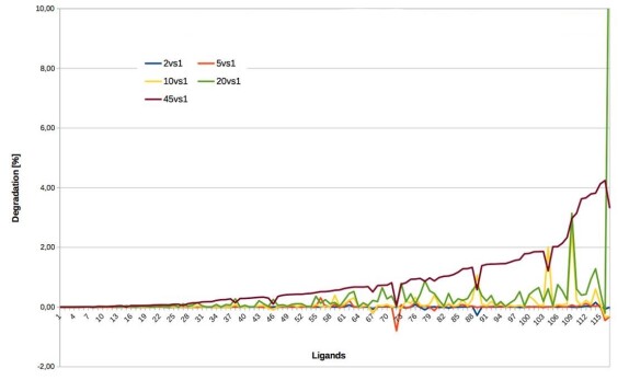
Our dataset is displayed in Figure 7, where molecules are ordered by increasing volume. The vertical axis shows the percentage of degradation in the molecular volume when the unfolding is made with an angle greater than 1 degree. The lines drawn in the plot identify granularities of 45, 20, 10, 5 and 2 degrees. The surprising result is that the degradation is always below 4% for rotations at 45 degrees with average around 1.7%.

For this reason, even though we introduced the possibility of using different angular discretisations, as shown in eq. 20, we focuses on a granularity of 45 degrees. The combinatorial optimization would only require 8 binary variables for each rotatable bond to identify its angle while keeping the final quality loss acceptably low.

VI.3 Threshold Approximation

The generation of the HUBO phase is one of the most computationally intensive, since we are using a symbolic framework. The challenges that arise are strictly related to the enormous amount of memory used and the unparalleled implementation of the symbolic engine. Hence, a straight derivation of the HUBO becomes unrealistic when increasing problem size.

For this reason, a last simplification was introduced, which consists in eliminating the optimization terms in 22 (only those not related to the hard constraints) whose coefficient is strictly less than a certain threshold value.

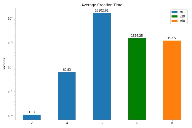
The effect of such threshold approximation (also called chop) was to speed up the computation of the HUBOs, as shown in Figure 8, and decrease the number of terms in the QUBO function in order to match the quantum annealing hardware specifications and limitations such as number of qubits (i.e. binary variables) and connectivity (i.e. quadratic terms) of the problem. Our study doesn’t go beyond the 8 rotatable bonds as HUBO construction involving 10 torsionals exceeded the time limit with the current setup and software.

Figure 8: Average creation time for HUBOs. We were able to generate HUBOs without the threshold approximation, up to 5 torsionals. In the case of 6 and 8 rotatable bonds, the threshold was increase to the vale of 30 and 60 respectively.

VII Altenative Search Strategies

In the following, classical optimization strategies used to compare quantum annealing results are presented.

VII.1 Random Search

Random Search Bergstra and Bengio (2012) algorithm works by picking up randomly the candidate solution from a uniform distribution. A big strength of this method is the high parallelization and the possibility of using Bayesian techniques or probability distributions that are more suitable for a given problem.

Algorithm 1 Random Search

1:$A\ =\ Angles,\ Poly=\ D_{ab}({\Theta})^{2},\ T=Torsional\ Bonds\ Set$ 

2:${\gamma_{max}}\mathrel{\mathop{\mathchar 58\relax}}\mathbf{max}\ D_{ab}({\gamma_{max}})^{2}$  

3:$|T|=m$  

4:$\Gamma\ =\ A_{1}\times A_{2}\times...\times A_{m}$  $\triangleright$ Cartesian product of the set of angles - m times.

5:while  $t\ <\ MaxTime$  do

6:   $\gamma=\ pick\_rand\_uniform(\ \Gamma\ )\$

7:   $Evaluate\ Poly(\Theta=\gamma)$  $\triangleright$ Evaluate assignments and record the optimum.

8:end while

9:return $[\ \gamma_{max},\ max\ Poly]$ 

VII.2 GeoDock Search

The GeoDock search is a greedy algorithm which considers a single torsional at a time and makes a decision locally for each rotatable bond. The algorithm usually does not lead to an optimal solution but it can reach good approximate solutions in a reasonable time.

This algorithm is the only one that is not employing symbolic computation. Each bond is rotated independently, starting from the most central and internal bond with respect to betweenness centrality. Only the conformation that improves the volume is recorded as a solution. The whole process is repeated a number of times or until a plateau in the improvement is reached.

Algorithm 2 GeoDock Search

1:$A\ =\ Angles,\ Poly=\ D_{ab}({\Theta})^{2},\ T=Torsional\ Bonds\ Set$ 

2:${a_{max}}\mathrel{\mathop{\mathchar 58\relax}}\mathbf{max}\ D_{ab}(a_{max})^{2}$  

3:$|T|=m$  

4:for  $t_{i},\theta_{i}\ in\ T_{ordered}$  do $\triangleright$ Ordered by betweenness centrality.

5:     for  $\ a\ in\ A\$  do

6:       $Evaluate\ Poly(\theta_{i}\ =\ a)$  $\triangleright$ Record intermediate optimums.

7:     end for

8:end for

9:return $[\ \underline{a}_{max},\ max\ Poly]$ 

VII.3 Simulated Annealing

Simulated annealing (SA) is a meta-heuristic technique, useful in the search of the optimum in large solution spaces.

Algorithm 3 Simulated Annealing

1:$A\ =\ Angles,\ Poly=\ D_{ab}({\Theta})^{2},\ T=Torsional\ Bonds\ Set,\ N_{max}\ =\ Total\ Iterations$ 

2:${a_{max}}\mathrel{\mathop{\mathchar 58\relax}}\mathbf{max}\ D_{ab}(a_{max})^{2}$  

3:$T\leftarrow T_{max}$

4:$a_{max}$ = NULL

5:while $T>T_{min}\ and\ N<N_{max}$ do

6:     $next$ = $pickNeighbour(T,best)$

7:     $\Delta E$ = $Poly(next)-Poly(a_{max})$

8:     $r$ = $randomNumberUniform(0,1)$

9:     if $\Delta E<0$ then

10:         $a_{max}=next$ $\triangleright$ The neighbour is accepted as the new optimum.

11:     else if  $r<e^{\frac{-\Delta E}{k_{b}*T}}$ then

12:         $a_{max}$ = $next$ $\triangleright$ Moving to a neighbour.

13:     end if

14:     $T$ = $geometricDecrease(T)$

15:end while

16:return $[\ \underline{a}_{max},\ max\ Poly]$ 

Since we can visualize the solution space as points belonging to a graph, SA starts with an initial guess $s_{c}=s_{i}$ with its evaluation $f(s_{i})$. If the neighbour has a lower evaluation, we take it as the current solution $s_{c}$. If the neighbour has a higher evaluation, we accept it with a probability written as:

$$P_{accept}=\min(1,\ e^{-\frac{Poly(neigh.)-Poly(s_{c})}{T}})$$ (25)

where T is the temperature that starts from a high value and decreases in time according to a cooling schedule. Since SA solves the QUBO formulations of our problems, this algorithm was taken as main comparison against Quantum Annealing.

VIII Problem Complexity and Embedding

VIII.1 Resources Estimation

Figure 9: Mean number of linear and non-linear terms in the HUBOs, obtained varying the number of torsionals and value of the approximation threshold .

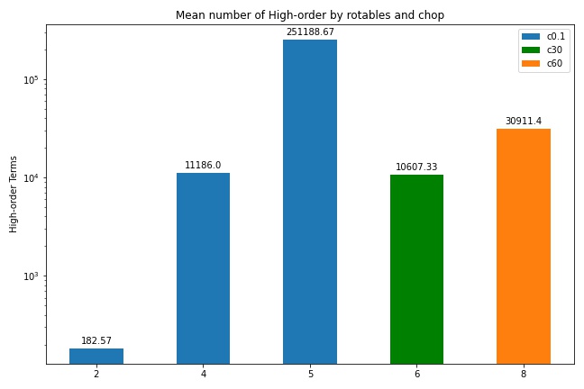
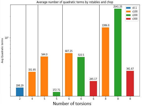
The metrics considered for evaluating the complexity of the problem are the number of linear and high-order terms appearing in the HUBO (plotted in Figure 9). The number of linear terms follows the relation $Number\ of\ rotatables\times\ granularity\ of\ rotation$. Recall that a granularity of 45 degrees was selected , i.e. $d=8$ in equation 20.

The number of non-linear terms grow rapidly going from 2 to 6 torsions. However, increasing problem size, the threshold approximation allowed us to avoid the exponential growth that these numbers would otherwise follow.

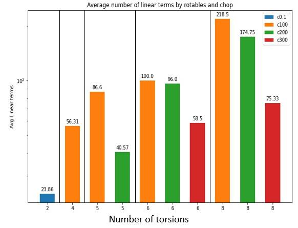
Since the final objective is to be able to embed our problems into a QPU, a second threshold approximations acting on the QUBO has been applied. The choice of the amount of chop is done by a fine tuning of the threshold, which is lowered until the embedding cannot be performed anymore.

The plots in Figure 10 show an increasing trend in the number of QUBO linear terms associated with the same threshold, for an increasing number of rotatables. Linear terms also decrease by increasing the threshold when the number of torsionals is fixed. Quadratic terms have a similar behaviour, except done for the class with 8 rotatable and a value for the approximating threshold set at 200, where more complex problems seem to peak.

Figure 10: Average number of linear and quadratic terms in the QUBOs, obtained varying the number of torsionals and value of the approximation threshold.

VIII.2 D-Wave Embedding

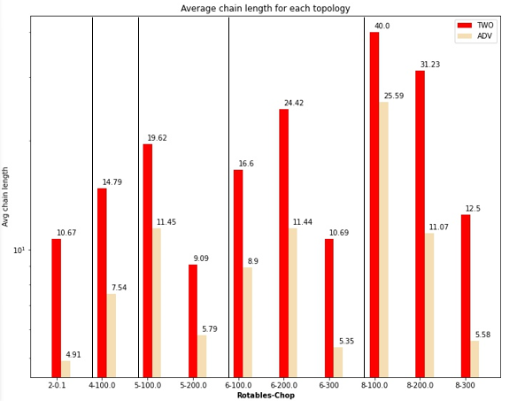
In the embedding phase, a heuristic algorithm tries to find the optimal matching between problem resources and physical D-Wave hardware. Several embedding are possible, so the one that uses the least physical qubits out of few trials is employed. It’s implicit in this choice that such embedding will also have shortest chains on average, i.e. chains of physical qubits representing a single QUBO variable.

The embeddings shown in Figure 11 are highly representative of the capabilities of each QPU topology. On average, the chains obtained with a Chimera topology are 2.09 times longer than those found using the Pegasus topology, which therefore returns 52% shorter chains.

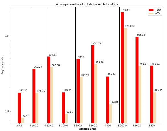
Regarding the number of qubits, Pegasus is again the winner as it enables embedding with 1.39 up to 2.4 times less qubits with respect to Chimera. On average, Advantage is 1.96 times more efficient than 2000Q, or 51% less expensive in terms of qubits; this will be reflected in the quality of results. There are only two results slightly diverging from our expectations. The columns regarding the class $6-100$ are shorter than expected because, due to the complexity of the problem, only simpler instances were embedded. Hence the average is biased towards a lower value.

There other important detail regards the class $8-100$ where both the average chain length and the average number of qubits are saturated to the maximum value for the 2000Q Chimera topology. This happened because the device couldn’t embed all the possible molecules for that class, therefore radically increasing the average.

Figure 11: Plots depicting the variation of average chain length and average number of qubits in the embeddings by increasing number of rotatables and value of the approximating threshold (also called chop)

IX Experimental Results

A short remark should be made on the way these algorithms run. Regarding the QA set-ups, since the QUBO constant $A_{const}$ modulating the strength of the hard constraint must be tuned, ten runs for each value assigned to $A_{const}$ are performed. $A_{const}$ is evaluated as the maximum coefficient in the optimization contribution multiplied by an increasing factor. Each run is performing ten thousands forward anneals with an annealing schedule of one microsecond. Simulated annealing is performed on the same QUBOs, with the possibility of choosing the number of epochs and the function which is responsible for the temperature decrease. In our case we used 500 annealing epochs and a geometrical decrease function.

Since executions of quantum and simulated annealing are repeated many times in the attempt of finding the best solution, also the other classical techniques are executed until their run-time does not exceed a time limit which was set from the beginning. Random search divides the solution space in N parallel processes and as long as it does not run out of time, it executes and records the maximal value found. The Geodock Search is trying an incremental approach, which consists in performing the rotation on an incremental number of bonds.

IX.1 Volume Gain in Time

Plots in the Figures 12 show the average trends in volume gain obtained by each algorithm on a fixed time window, increasing rotatable bonds. On the Y-axis, the maximum volume reached by every algorithm at each second is displayed. The plots show the algorithmic behaviour up to 100 seconds since this is the interval where greatest changes in volume appear.

Figure 12: Comparison of average volume gained on a time window of 100 seconds for 2, 4, 6 and 8 rotatable bonds.

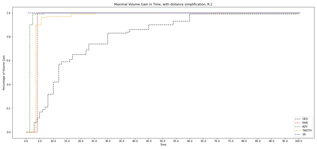
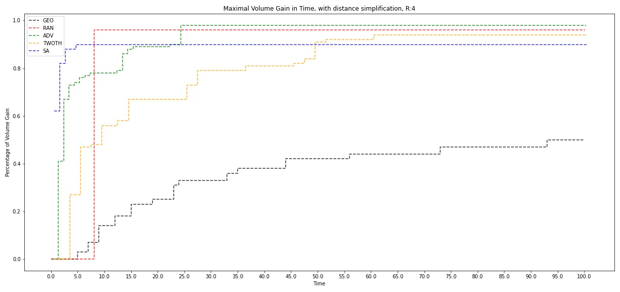
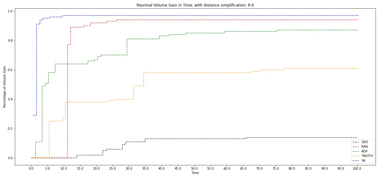
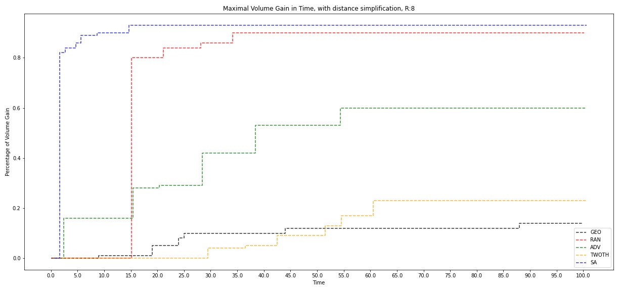
First thing worth noticing is that SA gave the best overall performance as it was able to provide good solutions falling inside the $[90\%,100\%)]$ volume gain range with a run-time that never exceeded the 15 seconds.

It is also possible to observe that Advantage is the best among D-Wave devices. For an increasing number of rotatable bonds, volume achieved by 2000Q quickly dies off, while the results of Advantage remain competitive for a good number of torsionals.

When 2 torsionals are considered, the MU problem looks like an easy task and basically all the approaches are able to recover the optimal solution (only GeoDock gets close but fails to find optimal). Random search, SA and the Advantage QA are able to reach the 100% volume gain within the first 5 seconds of runtime.

Increasing the problem size to 4 torsionals we can foresee a deviation of the trends: SA is again the fastest to reach a plateau while the quantum annealers perform better than random search in the first 5 seconds. After that, random search presents a disruptive improvement which comes with a delay due to overheads in the memory access. A promising result is obtained after 25 seconds, where Advantage is able to find the optimal solution among the methods. This indicates that QA could be a competitive approach when solving medium-small sized problems.

It is possible to see another reversal of the trends when the number of torsions rises to 6, in which SA and random search establish themselves as the most reliable solvers, followed by the Advantage quantum annealer. This behaviour is confirmed at 8 rotatable bond, where performances of 2000Q become very similar to that of the GeoDock greedy algorithm.

IX.2 Comparison between SA and QA

Comparing classical algorithms with quantum annealers in terms of absolute time isn’t fair, since the quantum devices have run-times that are comprising of programming time, readout time and delay time, besides the time spent in actually performing the annealing.

Therefore more suitable metrics for comparing annealing solvers is given by the Time To Solution (TTS),

$$TTS=\frac{total\ execution\ time}{occurrence\ of\ the\ best\ solution}$$ (26)

The total execution time can be calculated as the number of anneals multiplied by the total access time for single anneal. The occurrences of the best solution simply count the number of times the best solution is found in the annealing. The TTS metric can be interpreted as the inverse of the probability of finding the optimal configuration in a unit time interval. Moreover, the TTS is telling us how long we have to wait on average before the annealer outputs the best solution. For this reason, better solvers have low values of TTS.

Figure 13: A comparison between Simulated Annealing, Advantage and 2000Q on TTSs, for increasing number of torsionals.

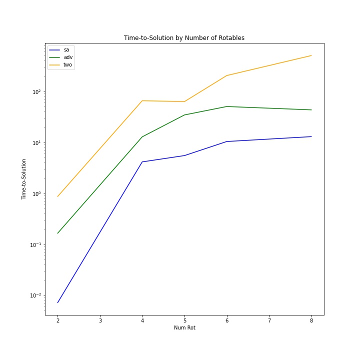
Plot in figure 13 show that the TTS is very high for 2000Q, followed by Advantage, while SA has the the best TTS. Simulated annealing has a TTS several times smaller than Advantage, which means that its convergence to the optimum is much faster than in quantum annealing.

Table 1: Comparison on the TTS, for increasing number of torsionals.

torsionals	sa	adv	two
2	0.007171	0.165081	0.868552
4	4.138503	12.818871	65.482955
5	5.502274	34.508321	62.996198
6	10.384806	50.430784	204.457250
8	12.942243	43.363135	503.938826

Regarding the volumes achieved, plots in Figure 14 represents the degradation in the final volume gain as the problem complexity increases. The volumes have a common starting point since all the three algorithm actually reach the maximum steadily and completely for problems involving 2 rotatable bonds. As seen in the previous section, Advantage works well up to 4 torsions, SA has an inflection on 4 bonds but then recovers and finishes as the best in absolute terms; it has a volume which is 4.65 times better than the one found by 2000Q at 8 bonds, and 1.4 times better than Advantage.

Figure 14: A comparison between Simulated Annealing, Advantage and 2000Q on volumes.

Table 2: Comparison on the Volumes, for increasing number of torsionals.

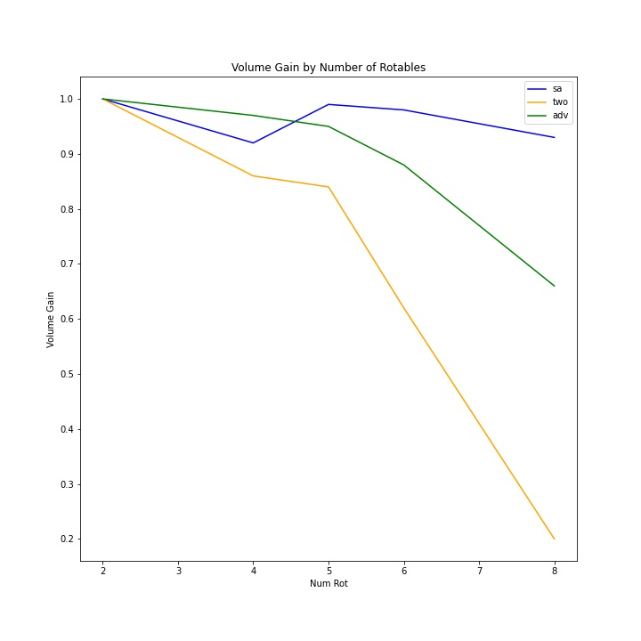
torsionals	sa	two	adv
2	1.00	1.00	1.00
4	0.92	0.86	0.97
5	0.99	0.84	0.95
6	0.98	0.62	0.88
8	0.93	0.20	0.66

The last concept worth mentioning is the measure of how much volume in percentage can be gained per unit of TTS. Practically, it is computed as the ratio between the normalized volume gain and TTS.

Figure 15: A comparison between Simulated Annealing, Advantage and 2000Q on the normalised decreasing quality of the volumes per time to solution.

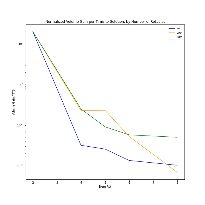
A negative slope in the plot of figure 15 can be interpreted as an increasing TTS required to achieve the same volume when scaling up to a more difficult problem. A higher negative slope means faster worsening of the algorithm with the increasing difficulty, while a smaller slope is a synonym of stability. Therefore, trends running towards the bottom of the plot belong to algorithms which are defective. The SA line falls down very fast from 2 to 4 torsionals, and then starts becoming stable. The same happens to Advantage which slows down this negative acceleration before. 2000Q never stops decreasing its quality, if not for a special case between 4 and 5 torsionals.

By checking the ratio of the slopes when increasing the number of torsionals, we can understand how much the algorithms are worsening adding degrees of freedom. On average the smallest growth in scaling of the slopes belongs to Advantage, with 1.36, whereas SA presents a higher 1.609, meanwhile 2000Q has an average of 6.01.

Although the results obtained with Advantage may not be the winners in absolute terms, the fact that Advantage has good performances with respect to SA according to this metric is a very promising. This result reflects how much QA is still immature but also how far from saturation the margin of growth for QA really is. Improvements in the next generation of QPU hardware could definitely affect both TTS and quality of sampling in a positive way.

Table 3: Average Normalized Volume Gain over TTS slopes for the three annealing algorithms.

sa	two	adv
1.609948	6.0189816	1.36206524

Table 4: Normalized Volume Gain over TTS for each algorithm, at different number of rotatable bonds.

sa	two	adv	torsionals
2.001031	2.000690	2.005038	2
0.003190	0.022822	0.025046	4
0.002582	0.023171	0.009112	5
0.001354	0.005269	0.005776	6
0.001031	0.000690	0.005038	8

X Conclusions

In this work, we explored the possibility of using a quantum annealer to support the drug discovery process within the in-silico virtual screening phase. In particular, we studied a new method regarding the process of molecular unfolding, which is the first step in geometric molecular docking techniques. This phase aims at finding the molecule’s configuration that maximizes its volume, or equivalently, that maximizes the internal distances of the atoms that compose the molecule. We proposed our Quantum Molecular Unfolding model with the aim of executing it on D-Wave’s latest hardware, Advantage and 2000Q. The usage of the quantum annealers has the objective of understanding the capabilities of these quantum annealing devices and discovering if it is possible to improve the quality and the throughput of the ligand expansion in the state-of-art molecular docking methods.

The model is constructed starting from the identification of the rotatable bonds which are the parameters of the problem. Once their discrete rotations are rewritten via one-hot encoding thanks to the introduction of binary variables, the total sum of internal atomic distances can be expressed as a HUBO. The HUBO is then transformed into a QUBO after three steps are applied: (i) distance simplification, (ii) coarse-grained rotations and (iii) threshold approximation. These three approximations enabled us to reduce the complexity of the model with the aim of embedding and running complex instances on the QPUs.

We compared the performances of Advantage and 2000Q, with three other optimization methods, which are parallel random optimization, simulated annealing, and a GeoDock greedy algorithm. The outcomes of the experiments show that Advantage have good performances on medium-small problems while classical techniques are better than quantum approaches when problem size increases. Interestingly, the results obtained by the quantum annealer, both while running on Advantage and 2000Q, are better than the GeoDock greedy approach. In terms of the evolution of the quantum annealers, embedding our problems on Advantage, compared to 2000Q, was on average 51% less expensive in terms of qubits and with chains 52% shorter. Advantage significantly outperforms 2000Q in terms of time-to-solution (TTS) and volume gain when increasing the number of torsionals. Advantage also presents the best scaling of the normalized volume gain over time-to-solution when compared to both 2000Q and simulated annealing; this last result is one of the most promising as D-Wave devices are only bound to get better.

Future work can be the introduction of new dynamic thresholds approximation, which may lead to smaller embeddings but still of high quality, and the introduction of hybrid quantum approaches. A more difficult but also feasible and interesting task could be extending the quantum annealing approach to the whole docking process. Finally, we are confident that this study will shed further light on the applications of quantum computing, thus enriching knowledge on topics that are becoming central in computational sciences.

Appendix

Machines and libraries

The platform used for running the classical algorithms is based on NUMA nodes, featuring 2 Intel(R) Xeon(R) CPU E5-2630 v3 CPUs (@2.40GHz), Virtualisation VT-x, caches L1d, L1i cache of 32K. L2 and L3 caches are, respectively, 256K and 20480K. RAM memory of 125 Gb and 114 Gb of SWAP memory. Operative system used is Ubuntu 18.04.5 LTS Bionic. The code was written in python 3.9.1, compiled with gcc 9.2.0. The parallelization was actuated with the usage of mpi4py 3.0.3, compiled with MPICH 3.3.2.

Since the classical probabilistic algorithms and random search, could be run in embarrassingly parallel mode, mpi4py [13] was used. For each problem instance, the number of processes used for each run was 32.

Other libraries of support are: Pandas 1.2.1, Numpy 1.19.5, symbolic calculations were performed thanks to Sympy 1.7.1 [14].

References

- Lyne [2002] P. D. Lyne, Drug Discovery Today 7, 1047 (2002), URL https://doi.org/10.1016/s1359-6446(02)02483-2.
- Meng et al. [2011] X.-Y. Meng, H.-X. Zhang, M. Mezei, and M. Cui, Current Computer Aided-Drug Design 7, 146 (2011), URL https://doi.org/10.2174/157340911795677602.
- Nielsen and Chuang [2010] M. A. Nielsen and I. L. Chuang, Quantum Computation and Quantum Information: 10th Anniversary Edition (Cambridge University Press, 2010).
- Preskill [2018] J. Preskill, Quantum 2, 79 (2018), ISSN 2521-327X, URL https://doi.org/10.22331/q-2018-08-06-79.
- McGeoch [2014] C. C. McGeoch (2014).
- Babej et al. [2018] T. Babej, C. Ing, and M. Fingerhuth, Coarse-grained lattice protein folding on a quantum annealer (2018), eprint 1811.00713.
- Marchand et al. [2019] D. J. J. Marchand, M. Noori, A. Roberts, G. Rosenberg, B. Woods, U. Yildiz, M. Coons, D. Devore, and P. Margl, Scientific Reports 9, 13708 (2019), ISSN 2045-2322, URL https://doi.org/10.1038/s41598-019-47298-y.
- Gadioli et al. [2020] D. Gadioli, G. Palermo, S. Cherubin, E. Vitali, G. Agosta, C. Manelfi, A. R. Beccari, C. Cavazzoni, N. Sanna, and C. Silvano, The Journal of Supercomputing 77, 841 (2020), URL https://doi.org/10.1007/s11227-020-03295-x.
- Kirkpatrick et al. [1983] S. Kirkpatrick, C. D. Gelatt, and M. P. Vecchi, Science 220, 671 (1983), URL https://doi.org/10.1126/science.220.4598.671.
- Mengoni et al. [2020] R. Mengoni, D. Ottaviani, and P. Iorio, arXiv preprint arXiv:2005.02268 (2020).
- Freeman [1977] L. C. Freeman, Sociometry 40, 35 (1977), URL https://doi.org/10.2307/3033543.
- Bergstra and Bengio [2012] J. Bergstra and Y. Bengio, J. Mach. Learn. Res. 13 (2012), ISSN 1532-4435.
- Dalcin et al. [2011] L. D. Dalcin, R. R. Paz, P. A. Kler, and A. Cosimo, Advances in Water Resources 34, 1124 (2011), URL https://doi.org/10.1016/j.advwatres.2011.04.013.
- Meurer et al. [2017] A. Meurer, C. P. Smith, M. Paprocki, O. Čertík, S. B. Kirpichev, M. Rocklin, A. Kumar, S. Ivanov, J. K. Moore, S. Singh, et al., PeerJ Computer Science 3, e103 (2017), URL https://doi.org/10.7717/peerj-cs.103.