Blueshifted hydrogen emission and shock wave of RR Lyrae variables in SDSS and LAMOST

Abstract

Hydrogen emissions of RR Lyrae variables are the imprints of shock waves traveling through their atmospheres. We develop a pattern recognition algorithm, which is then applied to single-epoch spectra of SDSS and LAMOST. These two spectroscopic surveys covered $\sim$ 10,000 photometrically confirmed RR Lyrae stars. We discovered in total 127 RR Lyrae stars with blueshifted Balmer emission feature, including 103 fundamental mode (RRab), 20 first-overtone (RRc), 3 double-mode (RRd), and 1 Blazhko type (temporary classification for RR Lyrae stars with strong Blazhko modulation in Catalina sky survey that cannot be characterized) RR Lyrae variable. This forms the largest database to date of the properties of hydrogen emission in RR Lyrae variables. Based on ZTF DR5, we carried out a detailed light-curve analysis for the Blazhko type RR Lyrae star with hydrogen emission of long-term modulations. We characterize the Blazhko type RR Lyrae star as an RRab and point out a possible Blazhko period. Finally, we set up simulations on mock spectra to test the performance of our algorithm and on the real observational strategy to investigate the occurrence of the “first apparition”.

1 Introduction

RR Lyrae stars are population II stars commonly found in globular clusters. They are located at the intersection of the instability strip and the horizontal branch (HB), from A- to F-type (Smith, 1995; Sesar, 2012). RR Lyrae variables are classified, according to the number of oscillation modes, as fundamental mode (RRab), the first overtone mode (RRc), or double-mode (RRd) stars (Soszyński et al., 2011). They obey the $M_{V}-[\mathrm{Fe/H}]$ relation (Muraveva et al., 2018) and the period-luminosity-metallicity relationship (PLZ, Longmore et al., 1986; Catelan et al., 2004) in the infrared passbands, which makes them good “standard candles” for precise distance determinations for star clusters and nearby galaxies (Bhardwaj, 2020). Some of the RR Lyrae variables, across all subtypes, show periodic amplitude and/or phase modulations, which is known as “Blazhko effect” (Blažko, 1907; Kolenberg et al., 2006).

Despite the successful application of RR Lyrae stars as a step of distance ladder, the detailed dynamical evolutions of the interior are unclear and complicated. However, we can speculate the internal structure of RR Lyrae variables by tracing the imprints of feature lines on spectra. Hydrogen emission lines, Helium emission lines, line broadening and doubling phenomena, neutral metallic line disappearance phenomena in RR Lyrae stars indicate shock waves propagating through their atmospheres (Chadid et al., 2017, 2008). The emissions are produced when atoms in the gas de-excite after being excited by a shock wave traveling into the atmosphere. The shock provides high enough energy to excite neutral hydrogen from the second quantum state upwards. It compresses, heats, and accelerates the gas. After that, the atoms release energy in the cooler shock wake region and generate the emission (Gillet & Fokin, 2014).

Hydrogen emission lines of RR Lyrae stars are called “apparitions” (Preston, 2011). There are three famous “apparitions”, which got their sequence number based on the discovery time. Sanford (1949) firstly reported a hydrogen emission in RR Lyrae in 1949. The “first apparition” is an intense blueshifted emission, which mostly presents during $\phi\approx 0.91$ (in RRab), just before the maximum luminosity (Gillet et al., 2019). Duan et al. (2021) reported the first detection of blueshifted hydrogen emission (the “first apparition” at both H$\alpha$ and H$\beta$) in the first-overtone and double-mode RR Lyrae variables. Now it is well accepted that the “first apparition” is generated from the hot emitting layer behind an outward-moving shock front (Schwarzschild, 1952).

The “second apparition” is a weak hump at the blue side of the absorption line wing, when $\phi\approx 0.73$, discovered in 1988 (Gillet & Crowe, 1988). It is generated by the collision when layers of the upper atmosphere meet the photospheric layers during the in-falling processes of the ballistic motion. It occurs during the small bump around $\phi\approx 0.72$, which was produced by the “early shock” (Hill, 1972; Gillet & Fokin, 2014). Moreover, the third one was discovered in 2011 (Preston, 2011), which is a weak redshifted emission line that appears at around $\phi\approx 0.30$. There are two views on the origin of the “third apparition”. One is that it is possibly provided by a weakly supersonic and infalling shock wave of post maximum (called $Sh_{PM}$), which is generated from superimposing compression due to hydrogen recombination front and the accumulations of weak compression waves (Chadid & Preston, 2013). The other opinion is that this emission is a P-Cygni like profile, which is the sign that the envelope surrounding the stellar surface is expanding, and the emission was produced when the shock wave is detached from the photosphere. To confirm which one is closer to the fact, further investigation is still needed.

Thanks to the rapid improvement of observing facilities, we can get an ever-expanding volume of observed spectroscopic data of RR Lyrae variables. In this work, we develop a pattern recognition searching algorithm and apply it to a large database of single-epoch spectra, the “first apparition”. We find out spectra of RR Lyrae stars which show most prominent observational characteristics of shock waves. We report hydrogen emissions in 103 RRab, 20 RRc, 3 RRd, and 1 Blazhko type RR Lyrae variables . The detection of blueshifted hydrogen emission in non-fundamental mode RR Lyrae variables has been discussed in our previous work (Duan et al., 2021). In this work, we present the results of RRab variables and the Blazhko type RR Lyrae star (RR-Bl, the Blazhko type RR Lyrae star with LAMOST spectra and hydrogen emission). The Blazhko type RR Lyrae star is characterized as an RRab star using pre-whitening sequence method. We build up the largest database of properties of the “first apparitions” in RR Lyrae stars based on SDSS and LAMOST, to investigate shock waves in RR Lyrae stars with a new view.

This paper is organized as follows. In Section 2, we describe the observations of both photometry and spectroscopy. The searching methods are interpreted in Section 3. We display the results of the search in Section 4. Moreover, we analyze the frequency components in RR-Bl, characterize it as an RRab star, and provide a possible Blazhko period in Section 5. The detection rate and mock spectra test are discussed in Section 6. Finally, the conclusions are covered in Section 7.

2 Observations

2.1 Photometric observations

Both photometric and spectroscopic observations are needed to hunt for the “first apparitions”. Light curves are used to identify RR Lyrae variables. They can be collected from the Catalina Sky Surveys, the Wide-field Infrared Survey Explorer (WISE), the All Sky Automated Survey for Supernovae (ASAS-SN) and the Asteroid Terrestrial-impact Last Alert System (ATLAS).

The Catalina Sky Survey began in 2004 (Drake et al., 2009). It uses three telescopes to cover the sky ($-75^{\circ}<\delta<+65^{\circ}$), in order to search for Near Earth Objects (NEOs) and Potential Hazardous Asteroids (PHAs). The sub-surveys are specified as the Catalina Schmidt Survey (CSS), the Mount Lemmon Survey (MLS) located in Tucson Arizona, and the Siding Spring Survey (SSS) which is located in Siding Spring Australia. In Catalina survey, RR Lyrae stars with strong Blazhko modulation are classified as “Blazhko type” other than the basic types (RRab, RRc, and RRd) of RR Lyrae variables, because the long-term modulation strongly influences the classification. Lots of photometric observations and analyses of RR Lyrae stars have been provided by related works (Drake et al., 2013b, a; Torrealba et al., 2014; Drake et al., 2014, 2017).

Moreover, the Wide-field Infrared Survey Explorer (WISE, Chen et al., 2018) is a 40 cm space telescope, designed to implement an all-sky survey in 4 MIR bands, including $W$1 (3.35$\mu$m), $W$2 (4.60$\mu$m), $W$3 (11.56$\mu$m) and $W$4 (22.09$\mu$m) (Wright et al., 2010). Chen et al. (2018) has compiled the first all-sky mid-infrared variable-star catalog based on WISE five-year survey data, providing 1231 RR Lyrae stars newly identified.

The All Sky Automated Survey for Supernovae (ASAS-SN, Shappee et al., 2014; Kochanek et al., 2017) is currently consisting of 24 telescopes around the globe. It is now automatically surveying the entire visible sky every night down to $\sim 18$ mag. Catalog from ASAS-SN (Jayasinghe et al., 2019) provides $\sim 412,000$ variables including $\sim 8000$ periodic pulsating stars.

The Asteroid Terrestrial-impact Last Alert System (ATLAS, Heinze et al., 2018) scans most of the sky every night to search dangerous asteroids, which is also used to search for photometric variability (Tonry et al., 2018). We also get light curves from the Zwicky Transient Facility (ZTF, Bellm et al., 2019; Masci et al., 2019; Chen et al., 2020) and parameters from Gaia DR2 (Clementini et al., 2019) for our selected stars if available.

2.2 Spectroscopic observations

Our spectroscopic data was collected from the Sloan Digital Sky Survey (SDSS) and the Large Sky Area Multi-Object Fiber Spectroscopic Telescope survey (LAMOST). In this work, we adopt low-resolution and single epoch spectra. The periods of RR Lyrae stars are very short. Under the circumstances, the emission features can be overwhelmed by long-time exposures and the processes of combining spectra to get a higher signal-to-noise ratio. Therefore, we use low-resolution and single epoch spectra to capture these features which will fast wear away otherwise.

The Sloan Digital Sky Survey (SDSS, Eisenstein et al., 2011) is one of the most ambitious surveys in the history of astronomy and enjoys enormous influence. It saw its first light in 1998 and entered routine observations in 2000. Using the Sloan Foundation 2.5m optical telescope (Apache Point Observatory, New Mexico), the SDSS serves images and spectra of the Northern sky, and currently extends to the Southern Sky using the 2.5m Du Pont optical telescope (Las Campanas Observatory, Chile). SDSS-III is a massive spectroscopic survey focusing on the distant universe, the Milky Way Galaxy, and extrasolar planetary systems (Eisenstein et al., 2011). As for the SDSS dataset, some of the spectra come from the BOSS survey (Dawson et al., 2013). Spectra from SDSS cover wavelength from 3800–9200 Å and those from BOSS have wavelength coverage of 3650–10400 Å. They achieve $R\sim 1500$ at 3800 Å and $R\sim 2500$ at 9000 Å. In this work, we use SDSS DR9 because we utilize parameter from the SEGUE Stellar Parameter Pipeline (SSPP, Lee et al., 2008)–DR9.

Large sky Area Multi-Object fiber Spectroscopic Telescope (LAMOST, Deng et al., 2012; Zhao et al., 2012; Cui et al., 2012) is a Chinese national scientific research facility. This survey is consisting of two major parts: the LAMOST ExtraGAlactic Survey (LEGAS) and the LAMOST Experiment for Galactic Understanding and Exploration (LEGUE). It sets up a spectroscopic survey of millions of objects in much of the northern sky and has great potential to survey a large volume of space efficiently. We apply for low-resolution and single exposure spectra in LAMOST DR6 ($R\sim 1800$). Each plate was observed more than 3 times for SDSS and 1-3 times for LAMOST survey. As for SDSS, the exposure time is 10-40 minutes each. And as for LAMOST, that is 10-30 minutes each. It provides the finest time resolution for RR Lyrae targets.

From this large database, we can screen out spectra of RR Lyrae stars. We cross-match the catalog of RR Lyrae stars and the dataset of spectra with topcat (Taylor, 2005) and apply for single-epoch spectra from LAMOST. We get single-epoch spectra of 3526 RR Lyrae stars from SDSS DR9 and 5571 RR Lyrae stars from LAMOST DR1–6. The Location of RR Lyrae stars of this sample are shown in Figure 1.

3 Methods

Based on the profiles of the “first apparitions”, we adapt two methods to search for this kind of feature. In this section, we will explain the technical details of the pipeline we use to catch the blueshifted hydrogen emission lines of RR Lyrae stars in a large sky survey database.

3.1 1D pattern recognition method

The normal practice to search for a target feature is to check the profiles of spectra visually. Due to rapid growth of datasets in size and complexity, data science is being introduced into astronomical studies (Pesenson et al., 2010; Baron, 2019). Pattern recognition means automated recognition of patterns and regularities in data. It has become a useful tool in fetching specific features and dealing with classification (Djorgovski et al., 2006).

Given that the profile we want is quite simple and clear, we adopt a 1D pattern recognition method with hand-crafted rules. We can trace the trend of the profile as an intense emission Gaussian-like profile at the shoulder of the blue wing of a Gaussian-like absorption line wing. Both emission and absorption signatures should be more significant than $2\sigma$.

We choose windows as 6540–6590 Å for H$\alpha$, 4840–4880 Å for H$\beta$. We presuppose that the minimum values in the selected windows indicate the location of Balmer absorption profiles. The adopted results at least show clear target patterns at H$\alpha$ and H$\beta$ simultaneously. Both emission and absorption components should contain at least two observational points. We apply the pipeline to our collected spectra sample, with visual checks to avoid a false negative.

3.2 Cross-correlation method

Given that the appearance of the emission lines introduces sudden change on the spectra, the cross-correlation method is also useful for selecting blueshifted hydrogen emissions (Yang et al., 2014). If there is not a “first apparition”, there should only be one wide absorption line of H$\alpha$ on the spectrum. On the contrary, there would be one additional emission line, which introduces a big difference in the shapes of two spectra. So if the difference between radial velocities is strangely large, there are possibly the “first apparitions”.

The cross-correlation method implemented here works as follows: We use the first observed spectrum in a pair as the template, while the second one is shifted by 1 km/s steps between -250 km/s to 250 km/s. The shifted template is linearly interpolated at the points of the wavelength of the observational spectrum to calculate the cross-correlation function. It shows the difference of radial velocities ($\Delta$RV) between two spectra when the cross-correlation function reaches its maximum. Here we provide the results of differences of radial velocities with H$\alpha$ line in Figure 2.

We locally normalize the spectra between $6540<\lambda<6590\AA$ by the fitting result of the continuum. The quantity $\sigma$ of the spectra is calculated from RMS of the spectra from the first and last 5 points, within which the spectra are continuum dominated. We adopted results with both spectra satisfying S/N ¿ 15, and the significance of the absorption line is over $3\sigma$. The distribution of $\Delta$RV for both SDSS and LAMOST dataset are visualized in Figure 2. We check for the blueshifted hydrogen emission when $|\Delta\mathrm{RV}|$ ¿ 100 km/s.

All of the selected results are produced by the 1D pattern recognition pipeline. The cross-correlation method provides 13 RRab stars, 1 RRc star for SDSS and 44 RRab stars, 3 RRc stars, 1 RRd star and 1 Blazhko type RR Lyrae star for LAMOST. The distribution of $\Delta$RV for selected RR Lyrae stars are visualized in Figure 2. The cross-correlation method does help but not all of the spectra with emission show high $\Delta$RV, and not all spectra with high $\Delta$RV show emission. So our work is mainly based on the 1D pattern recognition pipeline. The cross-correlation method is used as a supplement.

4 Results

As the result, we find 33 RRab stars and 10 RRc stars in SDSS, 70 RRab stars, 10 RRc stars, 3 RRd stars and 1 Blazhko type RR Lyrae star in LAMOST that show the “first apparition”. Visualization of the spatial distribution of the selected stars is shown in Figure 1. The detailed analyses of the results of RRc and RRd stars has been demonstrated in Duan et al. (2021). In this paper, we present the measurements of RRab and Blazhko type RR Lyrae variables and compare the properties between different types of RR Lyrae stars.

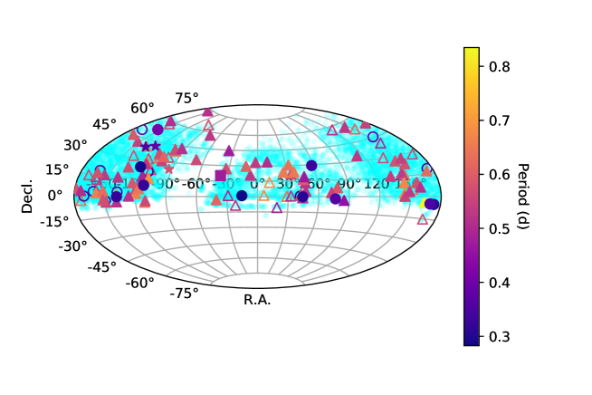
Figure 1: Spatial distribution of selected targets with the “first apparition”, with the color denoting the value of period. Corresponding relation: hollow triangle - RRab from SDSS, filled triangle - RRab from LAMOST, hollow circle - RRc from SDSS, filled circle - RRc from LAMOST, star - RRc from LAMOST, square - one Blazhko type star in LAMOST. Light blue points in the background denote the whole sample which our survey is based on.

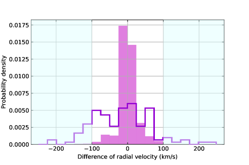
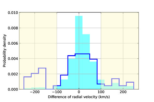
Figure 2: Distribution of the differences of radial velocities for SDSS (left) and LAMOST (right) respectively. The dataset was cleaned by S/N$\geq$15 and $3\sigma$ criteria. The filled histogram denotes the whole sample. The hollow histogram represents the distribution of the differences of radial velocities for the selected stars in this work. As for the cross-correlation method, we try to seek for the “first apparition” when $|\Delta\mathrm{RV}|$ ¿ 100 km/s.

The emission and absorption components are fitted with the $scale$ $width$ $versus$ $shape$ method for the hydrogen lines (Sersic, 1968; Clewley et al., 2002). We use two $S\acute{e}rsic$ functions (Xue et al., 2008; Yang et al., 2014; Duan et al., 2020) as:

$$y=m-ae^{-(\frac{\left|{\lambda}-{\lambda_{0}}\right|}{b})^{c}},$$ (1)

to fit the profile. Uncertainties are provided by error propagation with the covariance matrix and Monte Carlo method (Andrae, 2010).

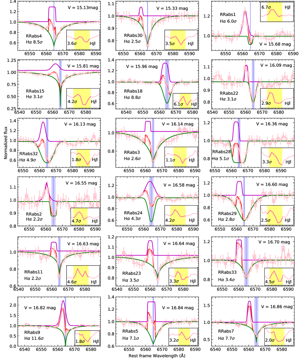
Figure 3: Visualization of examples of fitting results of RRab that show hydrogen emission in SDSS. The wavelength axis is in the stellar rest frame. The fitted blueshifted H$\alpha$ emission lines are shown as pink profiles. Green profiles denote fitted absorption lines. Red profiles represent the combination of fitted emission and absorption lines. Vertical blue lines denote the H$\alpha$ line laboratory wavelength. The H$\beta$ profiles are shown in the subplots. The significances of the emission lines denote the signal-to-noise ratio. The examples are ordered by $V$.

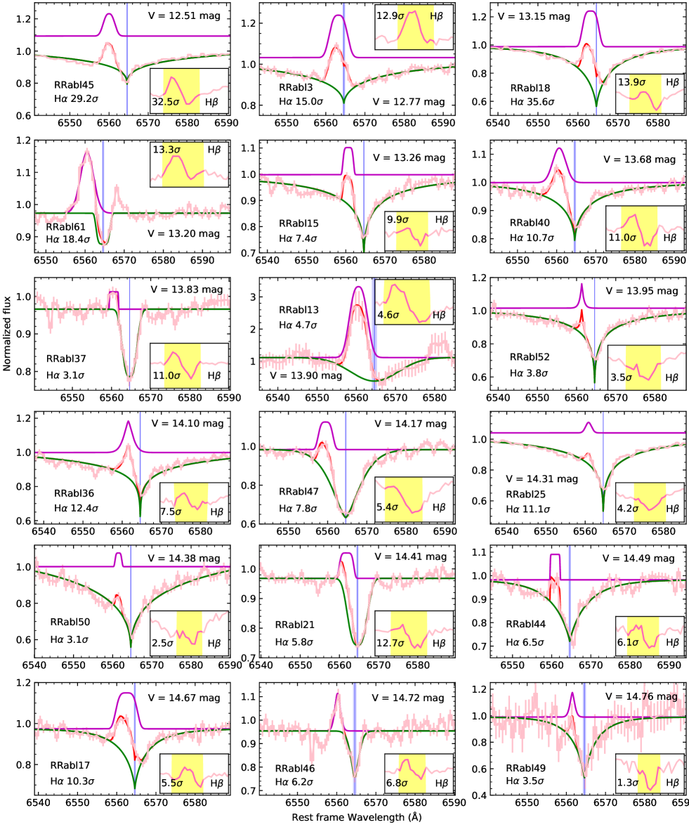
Figure 4: As Figure 3, but for selected RRab stars in LAMOST.

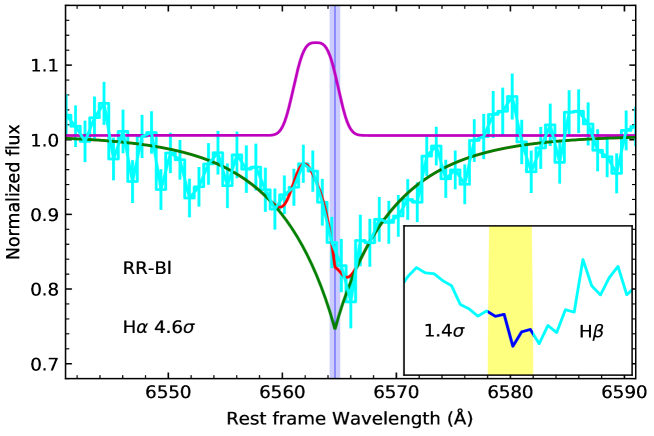
Figure 5: As Figure 3, but for a selected Blazhko type RR Lyrae star in LAMOST.

Figures 3 and 4 show the fitting examples of selected RRab stars in SDSS and LAMOST respectively, which display the blueshifted emission in H$\alpha$. Figure 5 shows the fitting result of the Blazhko type RR Lyrae star with the “first apparition” detected. The wavelength axis is in the stellar rest frame. Flux is normalized by continuum. The H$\alpha$ emissions are shown as pink profiles. H$\beta$ profiles are shown in the subplots. The significances of the blueshifted emissions for both H$\alpha$ and H$\beta$ are also shown. The candidates are adopted when the signals of H$\alpha$ is over $2\sigma$ and the signals of H$\beta$ is over $1\sigma$.

The radial velocity of the blueshifted hydrogen emission in the stellar rest frame is calculated as:

$$V_{\rm e1,\alpha}=c\frac{(\lambda_{\rm e1,\alpha}-\lambda_{\rm ab})}{\lambda_{0}},$$ (2)

where $\lambda_{\rm e1,\alpha}$ denotes the wavelength corresponding to the central wavelength of the emission line. $\lambda_{\rm ab}$ denotes the central wavelength of the absorption line. $\lambda_{0}$ denotes the laboratory wavelength.

We provide measurements of redshift $z_{\rm e1,\alpha}$ and radial velocity in the stellar rest frame $V_{\rm e1,\alpha}$, normalized flux Flux_e1,α and full width at half maximum (FWHM) of the emission and absorption FWHM_e1,α in the stellar rest frame of the blueshifted hydrogen emission. Parameters of the selected RR Lyrae variables and measurements of the “first apparitions” are summarized in Table 1, and 2. RR Lyrae stars with SDSS spectra that exhibit the first apparition are marked as RRabs (s as SDSS) and those with LAMOST spectra and hydrogen emission as RRabl (l as LAMOST). The star “RR-Bl” denotes the Blazhko type RR Lyrae star with LAMOST spectra and hydrogen emission (l as LAMOST). It was temporarily classified as a “Blazhko type RR Lyrae variable” because it was not accurately classified due to the significant modulation in the Catalina sky survey. In this work, RR-Bl is characterized as an RRab star using pre-whitening sequence method in Section 5.

Table 1: Parameters of selected RRab stars from SDSS.

Object	R.A.(J2000)	Decl.(J2000)	Period	$V$	Amp	$z_{\rm e1,\alpha}$	$V_{\rm e1,\alpha}$	Fluxe1,α	FWHMe1,α
	∘	∘	day	mag	mag		km/s		$\rm\mathring{A}$
RRabs1	$6.20764$	$+1.21571$	$0.68042$	$15.68$	$1.00$	$-4.72E-4\pm 1.86E-4$	$-141\pm 79$	$0.25$	$3.05$
RRabs2	$11.87371$	$+13.91740$	$0.69140$	$16.55$	$0.83$	$-6.35E-4\pm 1.87E-4$	$-190\pm 79$	$0.15$	$2.48$
RRabs3	$19.11867$	$-10.71342$	$0.48310$	$16.14$	$1.08$	$-4.84E-4\pm 1.88E-4$	$-145\pm 80$	$0.11$	$3.32$
RRabs4	$28.70903$	$+0.25027$	$0.63698$	$15.13$	$1.14$	$-1.68E-4\pm 1.87E-4$	$-50\pm 79$	$0.28$	$4.30$
RRabs5	$32.71725$	$+0.63203$	$0.51342$	$16.84$	$1.17$	$-1.77E-4\pm 1.87E-4$	$-53\pm 79$	$0.32$	$4.69$
RRabs6	$44.24281$	$-1.15499$	$0.51943$	$17.79$	$0.97$	$-5.76E-4\pm 1.88E-4$	$-173\pm 80$	$0.21^{*}$	$1.63$
RRabs7	$122.43165$	$+57.50441$	$0.52138$	$16.86$	$1.10$	$-6.37E-4\pm 1.85E-4$	$-191\pm 79$	$0.62$	$2.52$
RRabs8	$139.15997$	$+30.14284$	$0.57204$	$17.13$	$0.89$	$-2.75E-4\pm 1.88E-4$	$-82\pm 80$	$0.29$	$3.58$
RRabs9	$144.23392$	$+2.39681$	$0.68102$	$16.82$	$0.13$	$-2.16E-4\pm 9.45E-5$	$-65\pm 34$	$1.22$	$3.27$
RRabs10	$146.65068$	$+15.99970$	$0.52099$	$17.73$	$0.85$	$-1.92E-4\pm 1.86E-4$	$-57\pm 79$	$0.48$	$4.69$
RRabs11	$149.11227$	$+15.52289$	$0.65209$	$16.63$	$0.94$	$-5.20E-4\pm 1.86E-4$	$-156\pm 79$	$0.10$	$3.44$
RRabs12	$151.83224$	$+53.47885$	$0.61787$	$17.10$	$0.61$	$-3.41E-4\pm 1.15E-4$	$-102\pm 49$	$0.34$	$5.91$
RRabs13	$152.83864$	$+5.17696$	$0.64363$	$17.05$	$0.93$	$-2.46E-4\pm 1.85E-4$	$-74\pm 79$	$0.24$	$4.70$
RRabs14	$153.59429$	$+40.33244$	$0.49947$	$17.16$	$0.98$	$-4.67E-4\pm 1.88E-4$	$-140\pm 80$	$0.13$	$2.38$
RRabs15	$167.19900$	$-15.19530$	$0.57329$	$15.81$	$0.76$	$-4.55E-4\pm 9.61E-5$	$-136\pm 49$	$0.14$	$4.84$
RRabs16	$172.30798$	$+28.80851$	$0.56680$	$17.72$	$0.71$	$-2.95E-4\pm 1.85E-4$	$-89\pm 79$	$0.17$	$3.11$
RRabs17	$186.58595$	$-2.44612$	$0.62669$	$17.19$	$0.67$	$-2.68E-4\pm 6.97E-5$	$-80\pm 60$	$0.49$	$4.51^{*}$
RRabs18	$189.30895$	$+14.44229$	$0.57156$	$15.96$	$0.89$	$-1.81E-4\pm 1.86E-4$	$-54\pm 79$	$0.35$	$4.37$
RRabs19	$197.03942$	$+13.81974$	$0.51911$	$17.32$	$1.03$	$-2.64E-4\pm 1.88E-4$	$-79\pm 80$	$0.45$	$3.39$
RRabs20	$199.00117$	$+11.91443$	$0.52698$	$17.54$	$1.07$	$-7.74E-5\pm 6.52E-5$	$-23\pm 34$	$0.52$	$4.52$
RRabs21	$202.86013$	$+7.47637$	$0.54216$	$17.11$	$1.15$	$-4.81E-4\pm 1.00E-4$	$-144\pm 42$	$0.18$	$2.78$
RRabs22	$204.98954$	$+58.16789$	$0.57165$	$16.09$	$0.93$	$-6.40E-4\pm 1.88E-4$	$-192\pm 80$	$0.14$	$2.13$
RRabs23	$220.46840$	$+31.95186$	$0.57671$	$16.64$	$0.91$	$-6.96E-4\pm 1.87E-4$	$-209\pm 79$	$0.14$	$3.24$
RRabs24	$223.62869$	$+40.07005$	$0.66732$	$16.58$	$0.63$	$-1.32E-4\pm 1.87E-4$	$-40\pm 79$	$0.29$	$6.25^{*}$
RRabs25	$238.83554$	$+31.23341$	$0.56251$	$17.31$	$0.91$	$-2.78E-4\pm 1.87E-4$	$-83\pm 79$	$0.31$	$3.27$
RRabs26	$242.93547$	$+10.72981$	$0.55029$	$17.31$	$1.02$	$-5.83E-4\pm 1.14E-4$	$-175\pm 65$	$1.14^{*}$	$0.12$
RRabs$27_{1}$	$247.42582$	$+35.28750$	$0.63104$	$17.38$	$0.92$	$-3.45E-4\pm 1.88E-4$	$-103\pm 80$	$0.25$	$4.42$
RRabs$27_{2}$	$247.42582$	$+35.28750$	$0.63104$	$17.38$	$0.92$	$-3.82E-4\pm 1.54E-4$	$-115\pm 62$	$0.16$	$4.30$
RRabs28	$248.63333$	$+22.76128$	$0.55024$	$16.36$	$0.96$	$-2.63E-4\pm 1.86E-4$	$-79\pm 79$	$0.21$	$3.63$
RRabs29	$249.81254$	$+32.90717$	$0.63611$	$16.60$	$0.91$	$-4.49E-4\pm 1.88E-4$	$-135\pm 80$	$0.23$	$3.42$
RRabs30	$259.17579$	$+34.27990$	$0.57687$	$15.33$	$0.75$	$-6.08E-4\pm 1.87E-4$	$-182\pm 79$	$0.07$	$2.01$
RRabs31	$261.94862$	$+65.60181$	$0.57442$	$17.32$	$0.55$	$-3.66E-4\pm 2.27E-5$	$-110\pm 56$	$0.77$	$3.13$
RRabs32	$331.06979$	$+0.96542$	$0.50032$	$16.13$	$0.71$	$-3.76E-4\pm 4.50E-5$	$-113\pm 37$	$0.39$	$3.26$
RRabs33	$338.12842$	$-8.48267$	$0.52279$	$16.70$	$1.09$	$-6.80E-4\pm 1.87E-4$	$-204\pm 79$	$0.21$	$3.38$

Table 2: Parameters of selected RRab and Blazhko type stars from LAMOST.

Object	R.A.(J2000)	Decl.(J2000)	Period	$V$	Amp	$z_{\rm e1,\alpha}$	$V_{\rm e1,\alpha}$	Fluxe1,α	FWHMe1,α
	∘	∘	day	mag	mag		km/s		$\rm\mathring{A}$
RRabl1	$26.68188$	$+23.58775$	$0.65160$	$17.01$	$0.90$	$-5.04E-4\pm 9.89E-5$	$-151\pm 42$	$0.14$	$1.62$
RRabl2	$33.40705$	$+30.47452$	$0.63676$	$15.73$	$0.57$	$-5.33E-4\pm 3.86E-5$	$-160\pm 17$	$0.14$	$1.92$
RRabl3	$34.39211$	$+21.71650$	$0.56668$	$12.77$	$0.67$	$-2.11E-4\pm 1.51E-5$	$-63\pm 16$	$0.21$	$4.84$
RRabl4	$37.83211$	$+23.74759$	$0.64989$	$16.90$	$0.39$	$-4.69E-4\pm 9.87E-5$	$-141\pm 42$	$0.30$	$1.14$
RRabl$5_{1}$	$42.25593$	$+1.34632$	$0.57374$	$15.96$	$0.93$	$-6.09E-4\pm 9.87E-5$	$-183\pm 42$	$0.07$	$3.08$
RRabl$5_{2}$	$42.25593$	$+1.34632$	$0.57374$	$15.96$	$0.93$	$-3.71E-4\pm 4.08E-5$	$-111\pm 16$	$0.12$	$2.11$
RRabl6	$42.86087$	$+2.45366$	$0.61441$	$15.77$	$0.85$	$-7.48E-4\pm 4.53E-5$	$-224\pm 16$	$0.12$	$2.91$
RRabl7	$45.98163$	$+16.53199$	$0.59756$	$17.02$	$0.80$	$-6.27E-4\pm 9.93E-5$	$-188\pm 42$	$0.12^{*}$	$2.26$
RRabl8	$47.38816$	$+18.92607$	$0.47025$	$17.12$	$1.18$	$-4.77E-4\pm 5.94E-5$	$-143\pm 20$	$0.19$	$2.07$
RRabl9	$47.46535$	$+5.02683$	$0.51977$	$17.69$	$0.94$	$-5.86E-4\pm 4.94E-5$	$-176\pm 16$	$0.19$	$1.98$
RRabl10	$47.61406$	$+13.10191$	$0.52153$	$16.90$	$0.96$	$-5.63E-4\pm 9.89E-5$	$-169\pm 42$	$0.14$	$0.86$
RRabl$11_{1}$	$72.68140$	$+3.79305$	$0.55219$	$16.11$	$0.77$	$-2.36E-4\pm 2.62E-5$	$-71\pm 21$	$0.30$	$4.65$
RRabl$11_{2}$	$72.68140$	$+3.79305$	$0.55219$	$16.11$	$0.77$	$-2.77E-4\pm 8.91E-5$	$-83\pm 40$	$0.44$	$3.76$
RRabl$12_{1}$	$78.84653$	$+8.10691$	$0.59066$	$16.62$	$0.63$	$-6.09E-4\pm 4.73E-5$	$-183\pm 31$	$0.51$	$3.85$
RRabl$12_{2}$	$78.84653$	$+8.10691$	$0.59066$	$16.62$	$0.63$	$-6.15E-4\pm 4.99E-5$	$-184\pm 33$	$0.45$	$3.63$
RRabl13	$84.93823$	$-3.42164$	$0.45415$	$13.90$	$1.07$	$-6.20E-4\pm 2.21E-5$	$-186\pm 31$	$2.20$	$5.00$
RRabl14	$113.32693$	$+34.50516$	$0.53281$	$16.64$	$0.88$	$-4.31E-4\pm 3.47E-5$	$-129\pm 31$	$0.25$	$2.38$
RRabl15	$134.54286$	$+15.80513$	$0.54316$	$13.26$	$0.76$	$-6.08E-4\pm 9.87E-5$	$-182\pm 42$	$0.10$	$2.68$
RRabl$16_{1}$	$144.36704$	$+56.59926$	$0.52854$	$16.67$	$0.94$	$-5.50E-4\pm 9.89E-5$	$-165\pm 42$	$0.22$	$2.45$
RRabl$16_{2}$	$144.36704$	$+56.59926$	$0.52854$	$16.67$	$0.94$	$-5.11E-4\pm 9.89E-5$	$-153\pm 42$	$0.19$	$0.76$
RRabl$16_{3}$	$144.36704$	$+56.59926$	$0.52854$	$16.67$	$0.94$	$-4.62E-4\pm 2.50E-5$	$-138\pm 18$	$0.28$	$0.26$
RRabl17	$144.45373$	$+0.16152$	$0.55127$	$14.67$	$0.99$	$-3.23E-4\pm 3.80E-5$	$-97\pm 16$	$0.18$	$5.52$
RRabl18	$145.76492$	$+10.31705$	$0.67384$	$13.15$	$0.73$	$-2.21E-4\pm 1.43E-5$	$-66\pm 8$	$0.25$	$4.20$
RRabl19	$147.23862$	$+17.52836$	$0.53657$	$15.85$	$1.06$	$-5.78E-4\pm 9.89E-5$	$-173\pm 42$	$0.16$	$2.65$
RRabl20	$148.41207$	$+26.51218$	$0.57894$	$17.06$	$0.76$	$-2.85E-4\pm 5.56E-5$	$-85\pm 34$	$0.30$	$5.33$
RRabl21	$149.35586$	$+3.66790$	$0.53401$	$14.41$	$1.04$	$-4.24E-4\pm 2.76E-5$	$-127\pm 14$	$0.09$	$3.69$
RRabl22	$156.00410$	$+23.57355$	$0.57618$	$16.23$	$0.87$	$-6.83E-4\pm 3.16E-5$	$-205\pm 32$	$0.21$	$3.74$
RRabl23	$156.42426$	$+27.70770$	$0.54505$	$17.72$	$1.01$	$-1.43E-4\pm 3.55E-5$	$-43\pm 27$	$0.43$	$3.96$
RRabl24	$158.23468$	$+9.95462$	$0.57453$	$15.13$	$0.71$	$-5.07E-4\pm 4.13E-5$	$-152\pm 26$	$0.13$	$2.83$
RRabl25	$160.76055$	$+6.57957$	$0.51591$	$14.31$	$0.78$	$-5.71E-4\pm 3.26E-5$	$-171\pm 10$	$0.07$	$1.77$
RRabl26	$163.78099$	$-3.94871$	$0.83472$	$15.20$	$1.19$	$-2.70E-4\pm 2.50E-5$	$-81\pm 11$	$0.13$	$5.09$
RRabl27	$172.95127$	$+16.94800$	$0.62769$	$15.56$	$0.87$	$-5.17E-4\pm 9.93E-5$	$-155\pm 42$	$0.11$	$2.59^{*}$
RRabl28	$186.22131$	$+3.89524$	$0.50837$	$16.62$	$0.98$	$-6.40E-4\pm 9.87E-5$	$-192\pm 42$	$0.12$	$1.87$
RRabl29	$190.79904$	$+44.92621$	$0.59282$	$15.56$	$0.96$	$-2.05E-4\pm 5.82E-5$	$-61\pm 34$	$0.33$	$10.26$
RRabl30	$196.40574$	$+59.99944$	$0.51326$	$15.42$	$1.11$	$-4.77E-4\pm 3.70E-5$	$-143\pm 14$	$0.11$	$3.35$
RRabl31	$196.74774$	$+16.74280$	$0.57767$	$17.35$	$0.55$	$-5.39E-4\pm 5.04E-5$	$-162\pm 19$	$0.27$	$2.60$
RRabl32	$201.57540$	$+2.64155$	$0.65792$	$14.97$	$0.83$	$-3.48E-4\pm 3.81E-5$	$-104\pm 29$	$0.23$	$3.57$
RRabl33	$204.94889$	$+15.59276$	$0.53250$	$15.04$	$1.09$	$-4.19E-4\pm 4.14E-5$	$-126\pm 19$	$0.18$	$4.34$
RRabl34	$207.17689$	$+41.91878$	$0.54509$	$15.27$	$0.91$	$-5.64E-4\pm 9.87E-5$	$-169\pm 42$	$0.16$	$2.28$
RRabl35	$207.84723$	$+3.96548$	$0.62922$	$15.22$	$1.06$	$-5.50E-4\pm 8.25E-5$	$-165\pm 25$	$0.07$	$3.69$
RRabl36	$208.18557$	$-2.30798$	$0.57549$	$14.10$	$1.04$	$-4.63E-4\pm 2.47E-5$	$-139\pm 10$	$0.18$	$2.44$
RRabl37	$211.07900$	$-4.10587$	$0.55437$	$13.83$	$0.90$	$-6.13E-4\pm 9.89E-5$	$-184\pm 42$	$0.05$	$2.36$
RRabl38	$219.15778$	$+14.79704$	$0.52376$	$15.85$	$1.00$	$-6.19E-4\pm 2.74E-5$	$-186\pm 10$	$0.18$	$1.02$
RRabl39	$221.29128$	$+1.50971$	$0.67651$	$14.97$	$0.89$	$-6.69E-4\pm 9.93E-5$	$-200\pm 42$	$0.08$	$2.42$
RRabl40	$221.37085$	$-4.02095$	$0.51691$	$13.68$	$0.96$	$-6.04E-4\pm 2.43E-5$	$-181\pm 11$	$0.12$	$3.90$

Object	R.A.(J2000)	Decl.(J2000)	Period	$V$	Amp	$z_{\rm e1,\alpha}$	$V_{\rm e1,\alpha}$	Fluxe1,α	FWHMe1,α
	∘	∘	day	mag	mag		km/s		$\rm\mathring{A}$
RRabl41	$224.32736$	$+22.98642$	$0.57342$	$15.42$	$0.92$	$-6.17E-4\pm 9.91E-5$	$-185\pm 42$	$0.07$	$2.56$
RRabl42	$233.40562$	$+0.43740$	$0.51954$	$15.78$	$0.82$	$-4.45E-4\pm 9.95E-5$	$-133\pm 42$	$0.11$	$2.86$
RRabl43	$235.23457$	$+10.96986$	$0.58815$	$15.29$	$0.79$	$-6.42E-4\pm 4.46E-5$	$-192\pm 14$	$0.06$	$2.28$
RRabl44	$239.16098$	$+4.04318$	$0.55646$	$14.49$	$0.81$	$-5.68E-4\pm 9.89E-5$	$-170\pm 42$	$0.11$	$2.52$
RRabl45	$239.38257$	$+28.63362$	$0.66540$	$12.51$	$0.53$	$-7.04E-4\pm 1.54E-5$	$-211\pm 9$	$0.14$	$3.18$
RRabl46	$240.30956$	$+2.61588$	$0.66357$	$14.72$	$1.00$	$-6.70E-4\pm 3.41E-5$	$-201\pm 22$	$0.16$	$1.61$
RRabl47	$240.35335$	$+27.02554$	$0.52700$	$14.17$	$0.84$	$-7.82E-4\pm 2.51E-5$	$-235\pm 11$	$0.14$	$3.78$
RRabl48	$242.48518$	$+6.42657$	$0.64348$	$15.75$	$0.88$	$-1.74E-4\pm 2.08E-5$	$-52\pm 15$	$0.25$	$4.26$
RRabl49	$242.93347$	$+17.00636$	$0.49055$	$14.76$	$1.04$	$-4.70E-4\pm 7.38E-5$	$-141\pm 29$	$0.19$	$1.31$
RRabl50	$245.90139$	$+36.42249$	$0.57302$	$14.38$	$1.12$	$-4.80E-4\pm 9.91E-5$	$-144\pm 42$	$0.08$	$1.70$
RRabl51	$249.52973$	$-3.43423$	$0.56249$	$14.86$	$1.00$	$-4.67E-4\pm 9.91E-5$	$-140\pm 42$	$0.10$	$0.98$
RRabl52	$250.09389$	$+15.06886$	$0.69196$	$13.95$	$0.74$	$-5.01E-4\pm 3.18E-5$	$-150\pm 10$	$0.15$	$0.75$
RRabl53	$253.42009$	$+34.38424$	$0.61463$	$15.56$	$0.53$	$-5.78E-4\pm 9.93E-5$	$-173\pm 42$	$0.16$	$1.34$
RRabl54	$254.49119$	$+30.71234$	$0.54937$	$16.84$	$0.91$	$-1.69E-4\pm 6.38E-5$	$-51\pm 33$	$0.43$	$3.93$
RRabl55	$259.42280$	$+41.32834$	$0.57087$	$14.77$	$0.86$	$-6.95E-4\pm 1.82E-5$	$-208\pm 8$	$0.15$	$3.43$
RRabl56	$261.66390$	$+40.15591$	$0.63667$	$17.75$	$0.94$	$-1.03E-4\pm 5.16E-5$	$-31\pm 31$	$0.41$	$7.09$
RRabl57	$266.22514$	$+42.81815$	$0.51673$	$15.43$	$1.02$	$-2.46E-4\pm 3.86E-5$	$-74\pm 15$	$0.17$	$4.38$
RRabl58	$319.48228$	$-3.03425$	$0.61376$	$15.60$	$0.44$	$-9.01E-4\pm 9.91E-5$	$-270\pm 42$	$0.13$	$0.91$
RRabl59	$347.44815$	$+29.67568$	$0.60791$	$16.68$	$0.63$	$-5.50E-4\pm 9.89E-5$	$-165\pm 42$	$0.07$	$1.72$
RRabl60	$352.58414$	$+21.11239$	$0.52758$	$14.91$	$0.97$	$-5.88E-4\pm 1.74E-5$	$-176\pm 7$	$0.17$	$2.44$
RRabl61	$357.69274$	$+33.35102$	$0.53392$	$13.20$	$0.77$	$-6.29E-4\pm 2.33E-5$	$-189\pm 15$	$0.19$	$3.95$
Object	R.A.(J2000)	Decl.(J2000)	Periodf	$G$	AmpG	$z_{\rm e1,\alpha}$	$V_{\rm e1,\alpha}$	Fluxe1,α	FWHMe1,α
	∘	∘	day	mag	mag		km/s		$\rm\mathring{A}$
RRabl62	$10.49515$	$+33.83455$	$0.50996$	$16.89$	$0.91$	$-6.51E-4\pm 1.49E-5$	$-195\pm 10$	$0.31$	$2.72$
RRabl$63_{1}$	$178.36094$	$+53.77534$	$0.54987$	$17.38$	$0.81$	$-5.60E-4\pm 2.04E-5$	$-168\pm 11$	$0.38$	$2.03$
RRabl$63_{2}$	$178.36094$	$+53.77534$	$0.54987$	$17.38$	$0.81$	$-5.72E-4\pm 9.89E-5$	$-171\pm 42$	$0.26$	$2.49$
RRabl64	$180.93050$	$+5.48829$	$0.57846$	$15.58$	$1.05$	$-3.50E-4\pm 3.28E-5$	$-105\pm 15$	$0.19$	$2.51$
RRabl65	$196.90430$	$+73.59784$	$0.51574$	$15.04$	$0.97$	$-4.89E-4\pm 2.84E-5$	$-147\pm 12$	$0.14$	$2.89$
RRabl66	$248.94414$	$-4.75558$	$0.66401$	$16.06$	$0.67$	$-1.35E-4\pm 9.81E-5$	$-41\pm 42$	$0.59$	$3.47^{*}$
RRabl67	$285.76599$	$+57.32673$	$0.52887$	$14.43$	$0.88$	$-2.74E-4\pm 2.58E-5$	$-82\pm 13$	$0.11$	$5.66$
RRabl68	$291.08516$	$+34.27314$	$0.56338$	$15.12$	$0.72$	$-5.80E-4\pm 5.86E-5$	$-174\pm 18$	$0.06$	$2.12$
RRabl69	$324.40104$	$+44.46210$	$0.47481$	$16.30$	$0.87$	$-5.72E-4\pm 9.91E-5$	$-171\pm 42$	$0.14$	$1.48$
RRabl$70_{1}$	$326.54851$	$+26.93884$	$0.57201$	$13.73$	$0.89$	$-6.67E-4\pm 2.53E-5$	$-200\pm 10$	$0.14$	$3.17$
RRabl$70_{2}$	$326.54851$	$+26.93884$	$0.57201$	$13.73$	$0.89$	$-2.49E-4\pm 1.43E-5$	$-75\pm 9$	$0.17$	$4.63$
Object	R.A.(J2000)	Decl.(J2000)	Period	$V$	Amp	$z_{\rm e1,\alpha}$	$V_{\rm e1,\alpha}$	Fluxe1,α	FWHMe1,α
	∘	∘	day	mag	mag		km/s		$\rm\mathring{A}$
RR-Bl	$322.09646$	$+20.22167$	$0.54283$	$14.84$	$0.41$	$-2.55E-4\pm 9.83E-5$	$-76\pm 42$	$0.12$	$3.98$

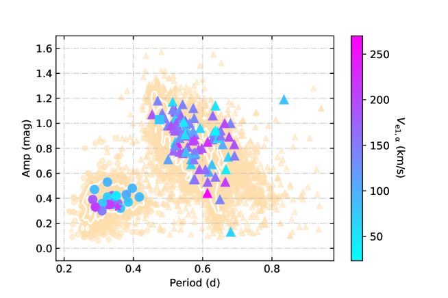
Figure 6: Period-Amplitude diagram. Selected stars with period and amplitude produced by Catalina Sky Survey are shown. Corresponding relation: triangle - RRab, circle - RRc, star - RRd, square - the Blazhko type RR Lyrae variable. The variation of color shows different absolute value of $V_{\rm e1,\alpha}$. Light yellow points in the background denote the whole sample of RR Lyrae stars. $1\sigma$ regions are shown as white contours.

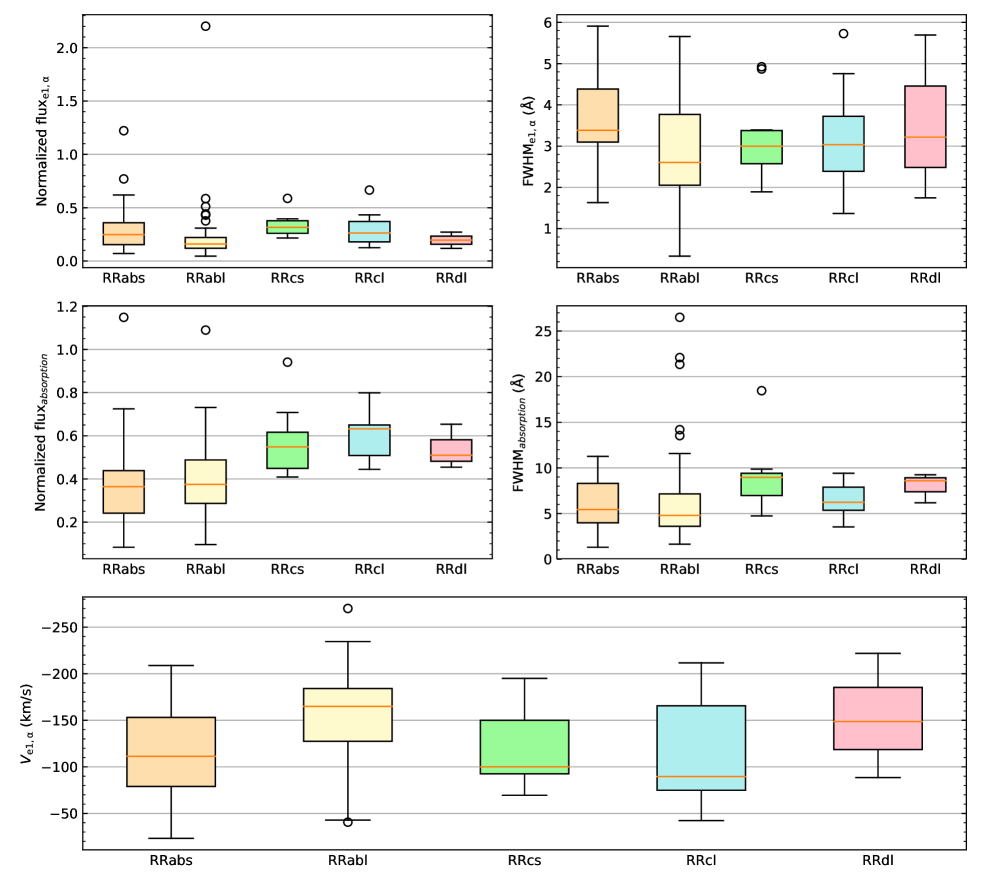
Figure 7: Box plots of measurements of different type of stars that show the “first apparitions”. Upper left (a): Normalized flux of emission (Flux_e1,α); Upper right (b): FWHM of emission (FWHM_e1,α); Lower left (c): Normalized flux of absorption; Lower right (d): FWHM of absorption. Bottom (e): $V_{\rm e1,\alpha}$ of different type of stars that show the “first apparition”.

The distribution of selected stars on Period-Amplitude diagram is shown in Figure 6. A clear gap divides RRab and RRc stars into two groups. RRab stars have longer periods and larger mean amplitudes than RRc stars. Box plots of the measurements are displayed in Figure 7. The mean value of normalized flux or FWHM of emission or absorption of RRc stars are higher than those of RRab stars. The mean value of $V_{\rm e1,\alpha}$ of RRab stars is higher than RRc stars.

Figure 8 shows the log $T_{\rm eff}$-log $g$ diagram. We adopt measurements of $T_{\rm eff}$ and log $g$ generated by SSPP if available. Despite the pipeline is not optimized for RR Lyrae stars and these values are derived from co-added spectra, the parameters from the pipeline can provide an overall description of log $g$-log $T_{\rm eff}$ distribution of various subgroups. Overall, RRc stars are hotter and have larger log $g$ than RRab stars. We also display simulated horizontal-branch (HB) evolutionary tracks for stars in the background, which was calculated with expansion and semiconvection of the core and enhanced oxygen composition from Dorman (1992), to show regions of different masses. The line consisting of red, green, and blue points in the background indicates evolutionary tracks for stars with $M=0.54,0.58,0.68M_{\odot}$, respectively.

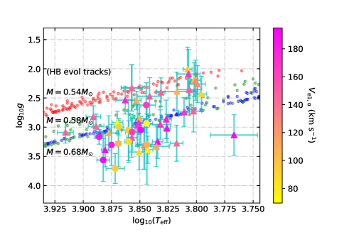
Figure 8: log $T_{\rm eff}$-log $g$ diagram for RR Lyrae stars that show the “first apparition”. Measurements of $T_{\rm eff}$ and log $g$ were produced by SSPP, if available. Points with error bars denote the selected stars with the “first apparitions”. Triangles denote RRab stars while circles denote RRc stars. The variations of color show different $V_{\rm e1,\alpha}$. The line consisting of red, green, and blue points in the background indicate the simulated horizontal-branch (HB) evolutionary tracks for stars with $M=0.54M_{\odot},0.58M_{\odot},0.68M_{\odot}$, respectively (Dorman, 1992).

The presence of the “first apparition” indicates a certain range of phase, just before the maximum luminosity. Figure 9 shows that points during a certain phase interval from RR Lyrae variables with similar properties is concentrating on a linear path on log $T_{\rm eff}$-log $g$ diagram when the effective temperature changes, which is demonstrated by a series of simulation using Modules for Experiments in Stellar Astrophysics (MESA, Paxton et al., 2019). We simulated 9 RRab and 9 RRc stars with various initial effective temperature in identical duration of evolution, while other initial parameters remain the same. The initial parameters are $M_{init}=0.55M_{\odot}$, $L_{init}=41.687L_{\odot}$, $X_{init}=0.736$ and $Z_{init}=0.008$, which indicates $[Fe/H]=-0.33$ (Das et al., 2018). $T_{eff}$ ranges from 6300K to 7100K in step width of 100K. In Figure 9, variation of color indicates the changing of luminosity, which can stand for the changing phase. Points at around $\phi=0.91$ locate on a linear path, highly characterized by Pearson correlation coefficients (PCC) as 1.000 and 0.999 for RRab and RRc respectively. The observation points on log $T_{\rm eff}$-log $g$ diagram have a diffuse distribution because our selected stars have various physical properties such as mass, luminosity, and metallicity. The different parameters make them deviate from one linear path.

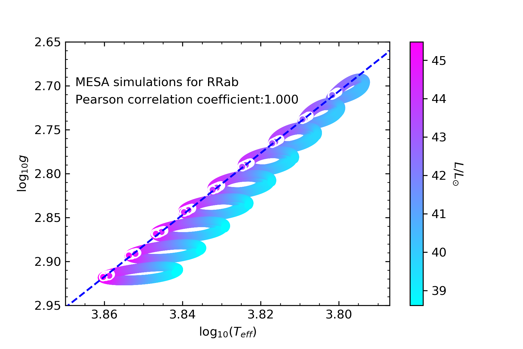
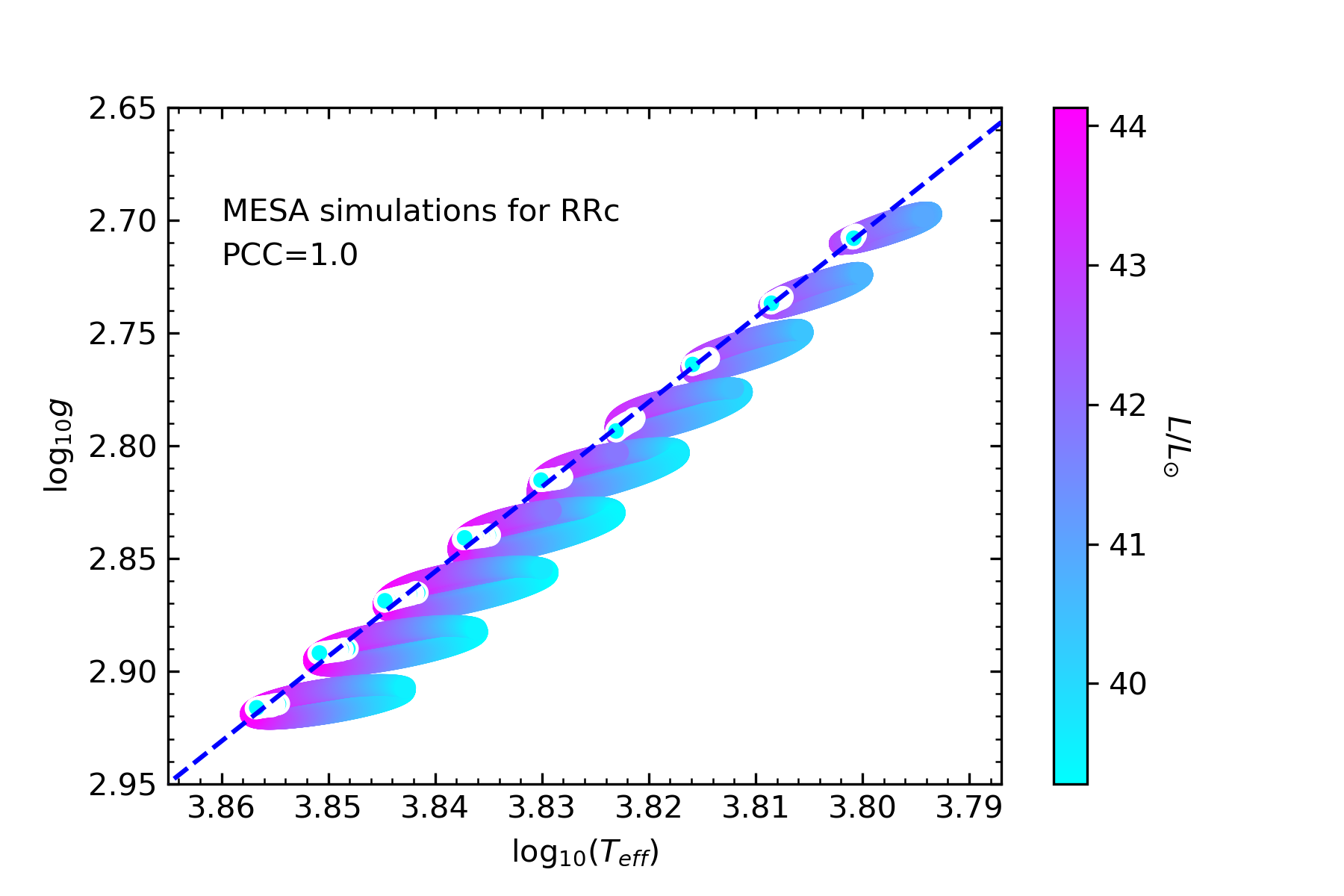
Figure 9: Left (a): log $T_{\rm eff}$-log $g$ diagram generated from MESA simulation for RRab and RRc stars. Left (a): Evolutionary tracks for a series of RRab stars during identical time intervals. The variations of color denote different $L/L_{\odot}$. The white points indicate the locations of $\phi=0.91$. The black dashed line show the linear fitting for the white points. As for initial parameters, $M_{init}=0.55M_{\odot}$, $L_{init}=41.687L_{\odot}$, $X_{init}=0.736$ and $Z_{init}=0.008$, which indicates $[Fe/H]=-0.33$. Initial $T_{\rm eff}$ ranges from 6300K to 7100K in step width of 100K. Right (b): Evolutionary tracks for a series of RRc stars during identical time intervals. Other comments are the same as Figure 9a.

5 Analysis of frequency components in the RR-Bl

We analyze $r$-band light curve of RR-Bl with a time span of 974.66 days with a standard successive pre-whitening method (Moskalik & Kołaczkowski, 2009). Observations in poor quality (catflags $\neq$ 0) have been removed. We fit the data using a non-linear least-square procedure with the sine series of the following form at each step:

$$m(t)=m_{0}+\sum^{N}_{k=1}A_{k}{\rm sin}(2\pi f_{k}t+\phi_{k}),$$ (3)

where $f_{k}$ denotes independent frequencies detected in discrete Fourier transform of the data and their possible linear combinations. The pre-whitening sequence for RR-Bl is shown in Figure 10. We find a $full$ $light$ $curve$ $solution$ for RR-Bl and produce the fitting results of the light curve in Figure 11.

According to $f_{0}=1.84226$, we derive the fundamental period $P_{0}=0.54281d$ and $A_{0}=0.242$ mag. Apart from $f_{0}$ and its linear combinations $nf_{0}$, we detect significant signals that can be expressed as $nf_{0}+\lambda_{c}f_{c}$, where $f_{c}\approx 1$, which can be explained as daily cadence. According to the pre-whitening sequence for RR-Bl, only one independent dominant frequency is detected. So RR-Bl is an RRab star with strong Blazhko effect.

The additional close side peaks at the fundamental frequency denote long-term modulation (Smolec et al., 2015). In Figure 12, the amplifying pattern is shown. The weak signatures beside $nf_{0}$ indicate a possible Blazhko-type modulation, with $f_{B}\approx 0.009$ and $P_{B}\approx 111.111{\rm d}$. The signals other than $f_{0}+f_{B}$ are not enough significant compared to others. Larger datasets are needed for a more precise analysis.

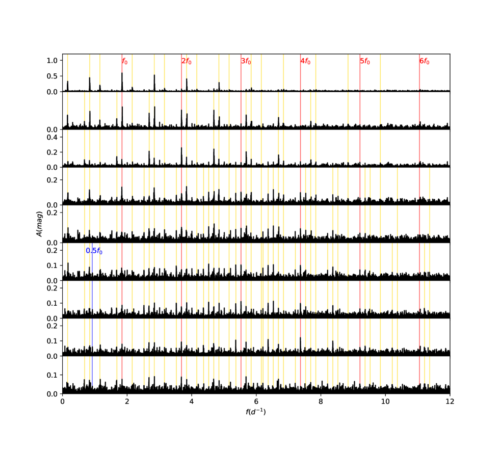
Figure 10: Pre-whitening sequence for RR-Bl. Uppermost panel displays power spectrum of the original data. Lower eight panels show power spectra after removing consecutive frequencies. $nf_{0}$ lines are marked with red color. $0.5f_{0}$ is marked with blue color. Yellow lines are linear combinations expressed by $nf_{0}+\lambda_{c}f_{c}$, while $f_{c}$ is the daily cadence.

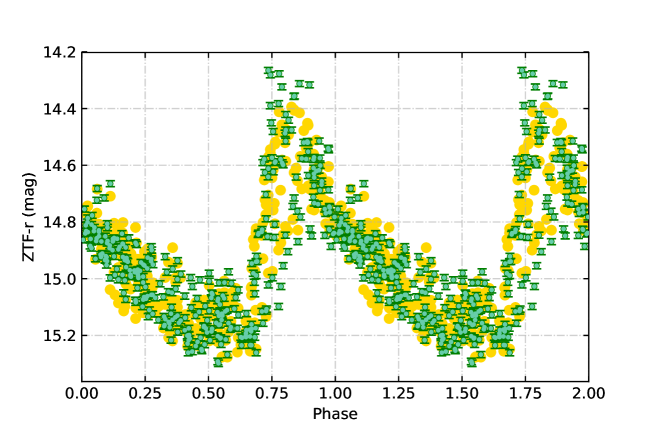
Figure 11: Regeneration of light curve of RR-Bl with full light curve solution. Green points with error bars are photometric observations from ZTF-r. Golden points are regenerated points with full light curve solution.

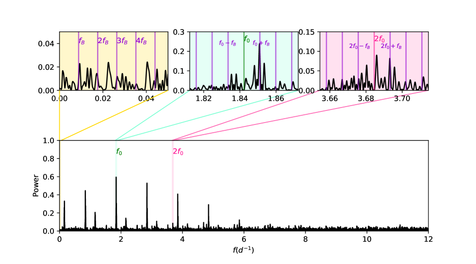
Figure 12: Pre-whitened power spectrum of RR-Bl. Lower panel displays power spectrum of the original data. Upper panels display power spectra after pre-whitening, showing the fine structures in low frequency, around $f_{0}$, and $2f_{0}$, respectively.

6 Detection rate and mock data test

The observational detection rate of blueshifted emission features in hydrogen lines of RR Lyrae stars is defined as:

$$\eta=\frac{\rm{N}_{obs}}{\rm{N}_{sat}},$$ (4)

where $\rm N_{\rm obs}$ represents the number of RRab stars featured emission components in LAMOST survey spectra. $\rm{N}_{sat}$ denotes the input number of RRab variables in the survey plan that are observed and with the S/N ratios of spectra greater than 15. Such definition of detection rate has an implicit assumption, that all RRab stars possess shock wave triggered emission, may or may not be detected in random sampling spectroscopic observations, depending on the observational timing and the strength of the emission feature.

The results of $\eta$ are: 1.84$\%$ - RRab in SDSS, 1.06$\%$ - RRc in SDSS, 2.87$\%$ - RRab in LAMOST, 1.45$\%$ - RRc in LAMOST, 2.97$\%$ - RRd and 2.56$\%$ for Blazhko type RR Lyrae star in LAMOST. The detection rate of the “first apparition” of RRc stars are significantly lower than RRab stars. We suggest that the detection rate in LAMOST are higher than those in SDSS is because that the sources in SDSS are fainter and the pixel resolution of LAMOST is higher than SDSS. As for SDSS, we choose the “spCFrame spectra”, the pixel resolutions are about 4150 at H$\alpha$ and 4180 at H$\beta$. As for LAMOST, the pixel resolutions are about 7800 at H$\alpha$ and 8400 at H$\beta$. The pixel resolution influences our results because one selecting criterion is that both emission and absorption components should contain at least two observational points. We set up two simulations for RRab variables in LAMOST: one on mock spectra to test the performance of our pipeline; the other on the observational strategy to investigate the occurrence of the “first apparition”.

Firstly, we test the performance of our pipeline on mock spectra generated based on the distributions of real observational parameters. We propose that the recognition rate of the shock wave signatures can be described as:

$$P(A)P(B\mid A)=P(AB),$$ (5)

where A = “the first apparition is observed on the spectra”, B = “the signal meets the criteria”. We recognize $P(A)$ as the real detection rate, while $P(AB)$ is the detection rate from the search. $P(AB)$ is lower than $P(A)$ due to finite S/N and our strict criteria of selecting the stars with the “first apparition”, which is described in Section 3.

We generate the mock spectra that have the “first apparition” and apply our 1D pattern recognition pipeline on the mock sample to estimate $P(B\mid A)$. The parametrizations of the simulated “first apparitions” are shown in Figure 13. The mock spectrum is regenerated as two Gaussian-like profiles between 6,540-6,590 $\rm\mathring{A}$. The central line of the absorption component is fixed at the rest wavelength of H$\alpha$. The blueshift of the emission, the ratio between the flux of emission and absorption component and the ratio between FWHM of emission and absorption component determine the shape of the simulated spectrum. The parameters of the Gaussian profiles are set as random values under Gaussian distribution based on the fitted distributions of the parameters of the selected RRab stars in LAMOST. Random noises are added up to the profiles to reproduce real situations, under Gaussian distribution where $\sigma$ is the error of normalized flux. The resolutions and S/Ns of mock spectra are taken from real observations.

We apply our pipeline on the mock sample and set up this simulation for 50 times. We only adopt the result of RRab stars in LAMOST. Because the pixel resolution of SDSS is low and the search in SDSS relies more on eye-checking. Moreover, the size of the sample of RRc, RRd and Blazhko type RR Lyrae star is not large enough to provide reliable parameter distribution. Figure 14 displays the results that $P(B\mid A)$ = 73.48% $\pm$ 0.43%. This means that, for a spectrum exhibiting blueshifted hydrogen emission with random flux, FWHM, and blueshift, there should be 73.48% $\pm$ 0.43% chance that our algorithm would recognize.

Secondly, we set up a following simulation on the real observational strategy to investigate the occurrence of “first apparition”. The simulation is based on the real parameters, including detection mode, exposure time, observation interval, observing frequency and the period of the corresponding RR Lyrae star for each spectra satisfying S/N ¿ 15.

In the simulation we preset that every star in the testing sample would have a “first apparition”. The exposure time for a spectrum with S/N ¿ 15 is then used as an observing window. Exposure times and observation intervals are obtained from real spectra. In the simulation, we set that the “first apparition” shows up for a short period of time before maximum luminosity in each pulsation cycle. Chadid (2011) reported that the “first apparition” appears over $\sim 5\%$ of the whole pulsation cycle. Gillet et al. (2019) reported that the “first apparition” presents during $\phi=0.892-0.929$ in RR Lyr, accounting for about $3.7\%$ of the whole period. Their researches are based on bright RR Lyrae stars. Our sample is much larger and contains a lot of faint stars. In the simulation, we assume that the “first apparition” accounts for about $4\%$ of the whole period.

As a matter of fact, too long-time exposures can smooth out the emission features in the hydrogen lines. Therefore we assume that the survival time of the emission feature and the exposure time should overlap with at least 70$\%$ of the exposure time for a clear signal. Each case that the emission overlaps with more than 70$\%$ of the exposure time yields one valid catch for a star. The number of valid catches of one star changes with observation time. The possibility of detecting a star with the “first apparition” is $P(B\mid A)$, $[1-(1-P(B\mid A))^{2}]$, or $[1-(1-P(B\mid A))^{3}]$ during the time when the star has one, two, or three valid catches, respectively.

As for the result, the number of detected RRab stars with blueshifted hydrogen emission in LAMOST from the simulation is about 371.79, while our observational result is 70. The result of the simulation is larger than our observational result. In our simulation we assume that every star in our sample exhibits the “first apparition”. However, not every RRab star has a visible “first apparition” in real survey due to variant shock strength. The occurrence of “first apparition” can be estimated as:

$$P(O)\rm{N}_{theo}=\rm{N}_{obs},$$ (6)

where O = “the star shows the first apparition”. We define $P(O)$ as the occurrence of “first apparition”. $\rm N_{\rm theo}$ is the number of detected RRab stars with blueshifted hydrogen emission in LAMOST from simulation. $\rm N_{\rm obs}$ denotes the number of detected RRab stars with blueshifted hydrogen emission in LAMOST in our survey. Here $\rm N_{\rm theo}=371.79$, $\rm N_{\rm obs}=70$, $P(O)$ $\approx$ 18.83%.

We suggest that $P(O)$ is underestimated. First, our simulation does not contain the selecting of H$\beta$ emissions due to the low resolution of the spectra, so $P(B\mid A)$ is overestimated. Another reason for the overestimation of $P(B\mid A)$ is that we used observed distribution but not the intrinsic distribution for emission flux. Moreover, in the progress of fitting we abandon some spectra which may show shock signatures but are hard to identify or provide no valid measurements, or contain no valid H$\beta$ emissions. That is to say, more than 18.83% of the RRab stars show relatively strong “first apparition”.

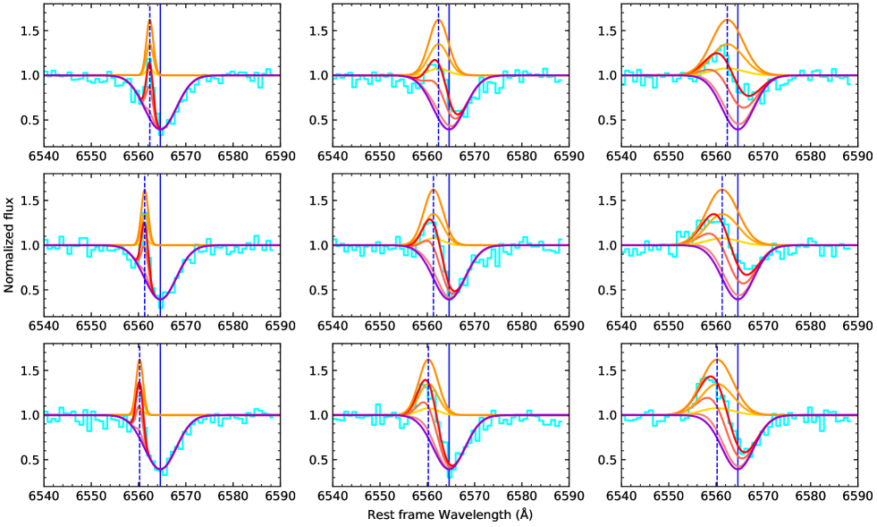
Figure 13: Simulated template of spectra of the “first apparitions”. The wavelength axis is in the stellar rest frame. The blueshifted H$\alpha$ emission lines are shown as orange profiles. The H$\alpha$ absorption lines are shown as blue profiles. Red profiles show the shapes of the “first apparitions”. Cyan profiles display the profile with random noises. Vertical blue solid lines denote the H$\alpha$ line laboratory wavelength. Vertical blue dashed lines denote the central wavelength of the emissions.

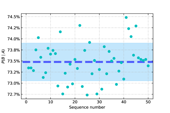
Figure 14: $P(B\mid A)$ of RRab stars in LAMOST.

7 Conclusions

In this work, we develop a hand-crafted 1D pattern recognition searching algorithm and apply it to a large dataset of single-epoch spectra of RR Lyrae stars, in order to fetch out the “first apparitions”. Through this survey, we found 33 RRab stars and 10 RRc stars in SDSS, 70 RRab stars, 10 RRc stars, 3 RRd stars and 1 Blazhko type RR Lyrae star in LAMOST. Based on the searching results, we set up the first population study of the RR Lyrae variables showing hypersonic shock waves.

We build up the largest database of blueshifted hydrogen emission in RR Lyrae stars. The features of the “first apparitions” are fitted by two $S\acute{e}rsic$ profiles. We provide the redshift $z_{\rm e1,\alpha}$ and radial velocity in the stellar rest frame $V_{\rm e1,\alpha}$, normalized flux Flux_e1,α and full width at half maximum of the emission and absorption FWHM_e1,α in the stellar rest frame of the blueshifted hydrogen emission. The distribution of measurements for different types are compared. We provide detailed analysis for the light curve of the Blazhko type RR Lyrae star with ZTF DR5. We characterize this Blazhko type RR Lyrae star as an RRab star with strong Blazhko modulations with a possible Blazhko period $P_{B}\approx 111.111{\rm d}$.

Finally, we set up two simulations for RRab variables in LAMOST. As for the first one, we apply our algorithm on mock spectra to test the performance of our pipeline and to check the influence of the selecting criteria. The other simulation is based on the real observational strategy to investigate the occurrence of the blueshifted hydrogen emission in RRab variables in LAMOST. The result suggests that more than 18.83% of the RRab stars exhibit relatively strong “first apparition”. The nature of RR Lyrae variables will be more and more clear with enormous volume of upcoming observational data.

References

- Andrae (2010) Andrae, R. 2010, arXiv e-prints, arXiv:1009.2755
- Astropy Collaboration et al. (2018) Astropy Collaboration, Price-Whelan, A. M., Sipőcz, B. M., et al. 2018, AJ, 156, 123
- Baron (2019) Baron, D. 2019, arXiv e-prints, arXiv:1904.07248
- Bellm et al. (2019) Bellm, E. C., Kulkarni, S. R., Graham, M. J., et al. 2019, PASP, 131, 018002
- Bhardwaj (2020) Bhardwaj, A. 2020, Journal of Astrophysics and Astronomy, 41, 23
- Blažko (1907) Blažko, S. 1907, Astronomische Nachrichten, 175, 325
- Catelan et al. (2004) Catelan, M., Pritzl, B. J., & Smith, H. A. 2004, ApJS, 154, 633
- Chadid (2011) Chadid, M. 2011, Carnegie Observatories Astrophysics Series, ed. A. McWilliam, Pasadena, CA: The Observatories of the Carnegie Institution of Washington, 5
- Chadid & Preston (2013) Chadid, M., & Preston, G. W. 2013, Monthly Notices of the Royal Astronomical Society, 434, 552
- Chadid et al. (2017) Chadid, M., Sneden, C., & Preston, G. W. 2017, ApJ, 835, 187
- Chadid et al. (2008) Chadid, M., Vernin, J., & Gillet, D. 2008, A&A, 491, 537
- Chen et al. (2018) Chen, X., Wang, S., Deng, L., de Grijs, R., & Yang, M. 2018, ApJS, 237, 28
- Chen et al. (2020) Chen, X., Wang, S., Deng, L., et al. 2020, ApJS, 249, 18
- Clementini et al. (2019) Clementini, G., Ripepi, V., Molinaro, R., et al. 2019, A&A, 622, A60
- Clewley et al. (2002) Clewley, L., Warren, S. J., Hewett, P. C., et al. 2002, MNRAS, 337, 87
- Cui et al. (2012) Cui, X.-Q., Zhao, Y.-H., Chu, Y.-Q., et al. 2012, Research in Astronomy and Astrophysics, 12, 1197
- Czesla et al. (2019) Czesla, S., Schröter, S., Schneider, C. P., et al. 2019, PyA: Python astronomy-related packages, , , ascl:1906.010
- Das et al. (2018) Das, S., Bhardwaj, A., Kanbur, S. M., Singh, H. P., & Marconi, M. 2018, MNRAS, 481, 2000
- Dawson et al. (2013) Dawson, K. S., Schlegel, D. J., Ahn, C. P., et al. 2013, AJ, 145, 10
- Deng et al. (2012) Deng, L.-C., Newberg, H. J., Liu, C., et al. 2012, Research in Astronomy and Astrophysics, 12, 735
- Djorgovski et al. (2006) Djorgovski, S. G., Donalek, C., Mahabal, A., et al. 2006, arXiv:astro-ph/0608638
- Dorman (1992) Dorman, B. 1992, ApJS, 81, 221
- Drake et al. (2009) Drake, A. J., Djorgovski, S. G., Mahabal, A., et al. 2009, ApJ, 696, 870
- Drake et al. (2013a) Drake, A. J., Catelan, M., Djorgovski, S. G., et al. 2013a, The Astrophysical Journal, 765, 154
- Drake et al. (2013b) —. 2013b, The Astrophysical Journal, 763, 32
- Drake et al. (2014) Drake, A. J., Graham, M. J., Djorgovski, S. G., et al. 2014, ApJS, 213, 9
- Drake et al. (2017) Drake, A. J., Djorgovski, S. G., Catelan, M., et al. 2017, MNRAS, 469, 3688
- Duan et al. (2020) Duan, X.-W., Chen, X.-D., Deng, L.-C., et al. 2020, Communications of the Byurakan Astrophysical Observatory, 67, 181
- Duan et al. (2021) —. 2021, ApJ, 909, 25
- Eisenstein et al. (2011) Eisenstein, D. J., Weinberg, D. H., Agol, E., et al. 2011, AJ, 142, 72
- Gillet & Crowe (1988) Gillet, D., & Crowe, R. A. 1988, A&A, 199, 242
- Gillet & Fokin (2014) Gillet, D., & Fokin, A. B. 2014, A&A, 565, A73
- Gillet et al. (2019) Gillet, D., Mauclaire, B., Lemoult, T., et al. 2019, A&A, 623, A109
- Harris et al. (2020) Harris, C. R., Millman, K. J., van der Walt, S. J., et al. 2020, Nature, 585, 357
- Heinze et al. (2018) Heinze, A. N., Tonry, J. L., Denneau, L., et al. 2018, AJ, 156, 241
- Hill (1972) Hill, S. J. 1972, ApJ, 178, 793
- Hunter (2007) Hunter, J. D. 2007, Computing in science & engineering, 9, 90
- Jayasinghe et al. (2019) Jayasinghe, T., Stanek, K. Z., Kochanek, C. S., et al. 2019, MNRAS, 486, 1907
- Kochanek et al. (2017) Kochanek, C. S., Shappee, B. J., Stanek, K. Z., et al. 2017, PASP, 129, 104502
- Kolenberg et al. (2006) Kolenberg, K., Smith, H. A., Gazeas, K. D., et al. 2006, A&A, 459, 577
- Lee et al. (2008) Lee, Y. S., Beers, T. C., Sivarani, T., et al. 2008, AJ, 136, 2022
- Longmore et al. (1986) Longmore, A. J., Fernley, J. A., & Jameson, R. F. 1986, MNRAS, 220, 279
- Masci et al. (2019) Masci, F. J., Laher, R. R., Rusholme, B., et al. 2019, PASP, 131, 018003
- Moskalik & Kołaczkowski (2009) Moskalik, P., & Kołaczkowski, Z. 2009, MNRAS, 394, 1649
- Muraveva et al. (2018) Muraveva, T., Delgado, H. E., Clementini, G., Sarro, L. M., & Garofalo, A. 2018, MNRAS, 481, 1195
- Oliphant (2006) Oliphant, T. E. 2006, A guide to NumPy, Vol. 1 (Trelgol Publishing USA)
- Paxton et al. (2019) Paxton, B., Smolec, R., Schwab, J., et al. 2019, ApJS, 243, 10
- Pedregosa et al. (2011) Pedregosa, F., Varoquaux, G., Gramfort, A., et al. 2011, Journal of machine learning research, 12, 2825
- Pesenson et al. (2010) Pesenson, M. Z., Pesenson, I. Z., & McCollum, B. 2010, Advances in Astronomy, 2010, 350891
- Preston (2011) Preston, G. W. 2011, AJ, 141, 6
- Sanford (1949) Sanford, R. F. 1949, ApJ, 109, 208
- Schwarzschild (1952) Schwarzschild, M. 1952, Transaction of the IAU VIII, ed. P. Th. Oosterhoff, Cambridge University Press, 811
- Sersic (1968) Sersic, J. L. 1968, Atlas de Galaxias Australes
- Sesar (2012) Sesar, B. 2012, The Astronomical Journal, 144, 114
- Shappee et al. (2014) Shappee, B. J., Prieto, J. L., Grupe, D., et al. 2014, ApJ, 788, 48
- Smith (1995) Smith, H. A. 1995, RR Lyrae Stars, Cambridge Astrophysics Series, 27
- Smolec et al. (2015) Smolec, R., Soszyński, I., Udalski, A., et al. 2015, MNRAS, 447, 3756
- Soszyński et al. (2011) Soszyński, I., Dziembowski, W. A., Udalski, A., et al. 2011, Acta Astron., 61, 1
- Taylor (2005) Taylor, M. B. 2005, Astronomical Society of the Pacific Conference Series, Vol. 347, TOPCAT & STIL: Starlink Table/VOTable Processing Software, ed. P. Shopbell, M. Britton, & R. Ebert, 29
- Tonry et al. (2018) Tonry, J. L., Denneau, L., Flewelling, H., et al. 2018, ApJ, 867, 105
- Torrealba et al. (2014) Torrealba, G., Catelan, M., Drake, A. J., et al. 2014, Monthly Notices of the Royal Astronomical Society, 446, 2251
- Virtanen et al. (2020) Virtanen, P., Gommers, R., Oliphant, T. E., et al. 2020, Nature Methods, 17, 261
- Wright et al. (2010) Wright, E. L., Eisenhardt, P. R. M., Mainzer, A. K., et al. 2010, AJ, 140, 1868
- Xue et al. (2008) Xue, X. X., Rix, H. W., Zhao, G., et al. 2008, ApJ, 684, 1143
- Yang et al. (2014) Yang, F., Deng, L., Liu, C., et al. 2014, New A, 26, 72
- Zhao et al. (2012) Zhao, G., Zhao, Y.-H., Chu, Y.-Q., Jing, Y.-P., & Deng, L.-C. 2012, Research in Astronomy and Astrophysics, 12, 723