A multiwavelength analysis of the spiral arms in the protoplanetary disk around WaOph 6

Abstract

Context. In recent years, protoplanetary disks with spiral structures have been detected in scattered light, millimeter continuum, and CO gas emission. The mechanisms causing these structures are still under debate. A popular scenario to drive the spiral arms is the one of a planet perturbing the material in the disk. However, if the disk is massive, gravitational instability is usually the favored explanation. Multiwavelength studies could be helpful to distinguish between the two scenarios. So far, only a handful of disks with spiral arms have been observed in both scattered light and millimeter continuum.

Aims. We aim to perform an in-depth characterization of the protoplanetary disk morphology around WaOph 6 analyzing data obtained at different wavelengths, as well as to investigate the origin of the spiral features in the disk.

Methods. We present the first near-infrared polarimetric observations of WaOph 6 obtained with SPHERE at the VLT and compare them to archival millimeter continuum ALMA observations. We traced the spiral features in both data sets and estimated the respective pitch angles. We discuss the different scenarios that can give rise to the spiral arms in WaOph 6. We tested the planetary perturber hypothesis by performing hydrodynamical and radiative transfer simulations to compare them with scattered light and millimeter continuum observations.

Results. We confirm that the spiral structure is present in our polarized scattered light $H$-band observations of WaOph 6, making it the youngest disk with spiral arms detected at these wavelengths. From the comparison to the millimeter ALMA-DSHARP observations, we confirm that the disk is flared. We explore the possibility of a massive planetary perturber driving the spiral arms by running hydrodynamical and radiative transfer simulations, and we find that a planet of minimum 10 M_Jup outside of the observed spiral structure is able to drive spiral arms that resemble the ones in the observations. We derive detection limits from our SPHERE observations and get estimates of the planet’s contrast from different evolutionary models.

Conclusions. Up to now, no spiral arms had been observed in scattered light in disks around K and/or M stars with ages $<1$ Myr. Future observations of WaOph 6 could allow us to test theoretical predictions for planet evolutionary models, as well as give us more insight into the mechanisms driving the spiral arms.

1 Introduction

The study of protoplanetary disks provides insight into our understanding of the formation and early evolution of planets. Modern observational techniques have enabled significant progress to be made in this task. Recent observations in both scattered light and millimeter continuum have shown the striking frequency with which these disks present structures, such as gaps, rings, or spirals (e.g., Avenhaus et al., 2018; Long et al., 2018; Andrews, 2020; Cieza et al., 2020).

In particular, spiral arms have been observed in more than a dozen young disks, spanning from tens to hundreds of au. They have been found in scattered light (e.g., Muto et al., 2012; Wagner et al., 2015; Benisty et al., 2015; Stolker et al., 2016; Garufi et al., 2020; Muro-Arena et al., 2020), millimeter continuum (e.g., Pérez et al., 2016; Huang et al., 2018b; Rosotti et al., 2020), and more recently in CO gas emission (e.g., Tang et al., 2017; Kurtovic et al., 2018). However, for the disks that have been imaged at different wavelengths, some of these spirals are only present in either scattered light, and not in the millimeter continuum, or vice versa. The mechanisms that drive spiral arms in these disks are probably manifold, and they are a matter of debate in many individual cases.

Considering that planets are born in protoplanetary disks, the observed structures have been frequently linked with the presence of planets forming within the disk (e.g., Muto et al., 2012; Pohl et al., 2015; Dong et al., 2018a; Calcino et al., 2020; Ren et al., 2020). These planets perturb the disks via gravitational interactions, and these perturbations can cause the formation of spirals. In these cases, the planets cause spiral arms both in the interior and exterior of their own orbit. In particular, when the planet is fairly massive, it can trigger a secondary spiral arm on the inside of its orbit. For a planet of tens of M_Jup, the primary and secondary spiral arm reach approximately a $m=2$ (Dong et al., 2015). From such planet-driven spirals, we can study the mass and location of the potential planets. Another mechanism that can drive spiral arms is gravitational instability (GI, e.g., Goldreich & Lynden-Bell, 1965). This happens when the self-gravity perturbations in the disk dominate over the restoring forces of gas pressure and differential rotation (Toomre, 1964), which can be translated to the disk being gas rich and relatively massive with respect to its host star (M${}_{\mathrm{disk}}/{\mathrm{M}_{*}}\gtrsim 0.1$ Kratter & Lodato (2016)). Spiral arms generated by GI can allow one to better constrain the disk mass. A third possible cause for the presence of spiral structure is a flyby event of a close companion to the system (e.g., Cuello et al., 2019; Ménard et al., 2020) that perturbs the disk material causing over densities that form the spiral pattern. And finally, a combination of some of the physical processes described above has also been investigated (e.g., Pohl et al., 2015).

Distinguishing between the possible physical processes driving spiral structure in protoplanetary disks is not an easy task. In fact, measuring the disk gas mass alone is already challenging. Having a more comprehensive understanding of these disks can be useful to decipher between the physical processes that are taking place within them. One approach is to use multiwavelength observations to trace their different components. In particular, images obtained in scattered light are sensitive to micron-sized dust grains at the disk surface, which under typical disk conditions are very well coupled to the gas. Images at (sub)millimeter wavelengths, on the other hand, trace larger grains within the disk midplane, and they are less well coupled to the gas. Therefore, comparing images at these wavelengths with similar angular resolution can potentially reveal the different morphologies of different disk components. Actually, it may be possible to distinguish between planet- or GI-induced spirals by comparing scattered light and millimeter continuum observations, since dust trapping in spiral arms is likely to be more efficient in gravitationally unstable disks (Juhász et al., 2015; Dipierro et al., 2015). Previous studies have utilized observations in both near-infrared (NIR) and millimeter continuum to analyze the disks’ morphology, as well as the gas and dust distributions within them (e.g., van Boekel et al., 2017; Rosotti et al., 2020), however, so far there are only a handful of such works.

In this paper, we present NIR polarimetric observations of WaOph 6 obtained using the VLT/SPHERE instrument (Beuzit et al., 2019). These observations have a spatial resolution of $\sim$51 mas ($\sim$ 6 au), similar to that of the recent ALMA-DSHARP millimeter wavelength observations (Andrews et al., 2018, see Fig. 1). We report a NIR scattered light counterpart of the innermost spiral arms reported in Huang et al. (2018b). Additionally, we explore one of the scenarios that can give rise to the spiral pattern observed in the disk.

The paper is structured as follows: in Section 2 we introduce WaOph 6 and the previous studies on its disk. In Section 3 we describe our scattered light observations and data reduction procedure. Our results are presented in Section 4. We describe the modeling setup and the comparison between the simulations and the observations on Section 5. In Section 6 we discuss our results, and finally in Section 7 we summarize our findings and list our conclusions.

2 Stellar and disk properties

WaOph6 is a K6 star (Eisner et al., 2005), and member of the Ophiuchus moving group at a distance of 122.5 ${}^{+0.3}_{-0.2}$ pc (Gaia Collaboration et al., 2020) located near the L162 dark cloud. It was first identified as a suspected T Tauri star by Henize (1976), and then confirmed by Walter (1986). Here we constrain the stellar mass and age based on the updated photometry and Gaia parallax. We retrieved the full spectral energy distribution (SED) from Vizier and employed a Phoenix model of the stellar photosphere (Hauschildt et al., 1999) with effective temperature T${}_{\mathrm{eff}}=4200$ K (Eisner et al., 2005), surface gravity log(g)=-4.0, and an optical extinction $A_{V}=2.8\pm 0.3$ mag calculated from the V, R, and I photometric fluxes. We integrated the stellar model scaled to the average V magnitude and Gaia distance of 122.5 pc obtaining a stellar luminosity of L${}_{*}=1.91^{+0.70}_{-0.51}$ L_⊙. Then, we placed the source on the HR diagram and constrain a stellar mass M${}_{*}=0.7\pm 0.1$ M_⊙ and an age $t=0.6\pm 0.3$ Myr through different sets of PMS tracks (Parsec, MIST, Baraffe; Bressan et al., 2012; Choi et al., 2016; Baraffe et al., 2015) with error bars propagated from L_∗ and T_eff ($\pm$ 100 K).

The disk around WaOph 6 has been a common target for millimeter continuum surveys looking to constrain and characterize the structure in protoplanetary disks (e.g., Andrews & Williams, 2007; Andrews et al., 2009; Ricci et al., 2010; Andrews et al., 2018). Submillimeter Array (SMA) observations were used along with a parametric model to constrain density structure parameters (Andrews et al., 2009). The disk model that best fitted the thermal continuum data and spectral energy distribution (SED) was that of a flat cold disk with a total disk mass (gas $+$ dust-to-gas ratio of 1:100) of 0.077 $M_{\odot}$. With observations from the Australia Telescope Compact Array (ATCA), Ricci et al. (2010) analyzed and modeled the SED of WaOph 6, adopting a distance of $\sim$130 pc and an outer radius (R_out) interval of $175-375$ au, and they find dust mass estimates (M_dust) between $8\times 10^{-5}\,\mathrm{M}_{\odot}$ and $9.8\times 10^{-5}\,\mathrm{M}_{\odot}$, depending on the assumed dust size distribution power-law index ($q=2.5$ or $q=3$). More recently, WaOph 6 was observed by ALMA within the DSHARP program (Disk Substructures at High Angular Resolution Project, Andrews et al., 2018). These millimeter continuum observations showed that the disk has a set of symmetric spiral arms that extend to $\sim$70 au, a gap at 79 au and a bright ring at 88 au (Huang et al., 2018b). The disk has an inclination ($i$) of 47.3^∘ and a position angle (PA) of 174.2^∘ obtained from ellipse fitting on the dust continuum emission (see Huang et al., 2018a, for more details), and gas observations have shown that it suffers from mild molecular cloud contamination (Reboussin et al., 2015). We summarize the stellar and disk physical parameters in Table 1, where we include the different values for the disk mass found in the literature, as well as our own M_dust estimate obtained following the procedure described in Appendix A.

Up to now, only seven disks have been known to have spiral arms in millimeter continuum wavelengths: WaOph 6, Elias 27, IM Lup, HT Lup A, AS 205 N, MWC 758, and HD100453 (Huang et al., 2018b; Kurtovic et al., 2018; Dong et al., 2018a; Rosotti et al., 2020), and only the first three are single systems. Out of these three, only IM Lup has published polarized scattered light observations (Avenhaus et al., 2018), however, with no spiral arms visible at these wavelengths.

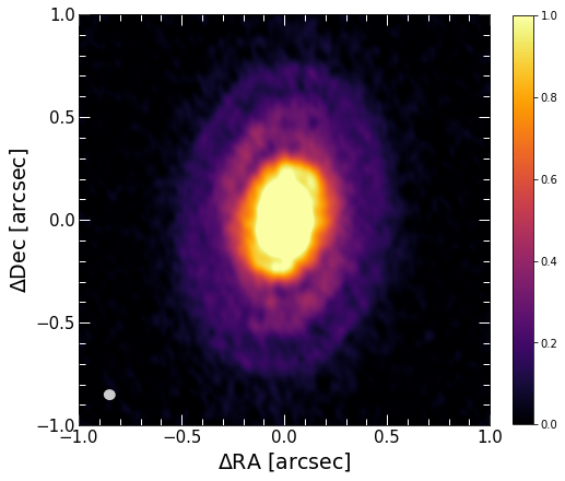
Figure 1: ALMA 1.25 mm continuum image of WaOph 6 from the ALMA-DSHARP survey (Huang et al., 2018b). The beam size is shown in the lower left corner.

Table 1: Stellar and disk parameters of WaOph 6 from the most recent literature.

Stellar parameters	Value	Ref.
Spectral type	K6	a
Age	0.7 Myr	a
Distance d	122.5 $\pm$ 5 pc	b
Mass	0.9 M⊙	a
Radius	2.8 R⊙	a
Temperature	4205 $K$	a
Visual magnitude ($V$ band)	13.3 $\pm$ 0.01 mag	c
Disk properties
Inclination i	47.3∘	d
Position angle (PA)	174.2∘	d
Gas mass	7.7x$10^{-2}$ M⊙	e
Dust mass	8x$10^{-5}$ M⊙	a
Dust mass	1.4x$10^{-4}$ M⊙	f

• Assuming a gas-to-dust ratio of 100:1 and based on SMA SED modeling.

• Obtained with a power-law index for the grain size distribution $q=2.5$.

• Notes.     a) Ricci et al. (2010), b) Gaia Collaboration et al. (2020), c) Zacharias et al. (2012), d) Huang et al. (2018a), e) Andrews et al. (2009), f) This work

Table 2: Log of observations.

Date	21-06-2018
Filter	$H$-band (1.625 $\mu$m)
UT start/end	01:58:36/02:24:30
Exposure time	96 s
Airmass	$\sim$1.0
Seeing	$\sim$ 0.5”
Coherence time ($\tau_{0}$)	$\sim$ 4 ms
Wind speed	$\sim$ 3.8 m/s
Total exposure time	$\sim$ 1500 s

3 Observations and data reduction

WaOph 6 was observed with the VLT/SPHERE high-contrast instrument (Beuzit et al., 2019) within the DISK/SHINE (SpHere INfrared survey for Exoplanets, Chauvin et al., 2017) Guaranteed Time Observations (GTO) program on the night of June 21, 2018 (see Table 2). The observations were carried out with the IRDIS Dual-beam Polarimetric Imaging (DPI) mode (Langlois et al., 2014; de Boer et al., 2020; van Holstein et al., 2020) in $H$-band ($\lambda_{c}$=1.625 $\mu$m; $\Delta\lambda$=0.291 $\mu$m; where $\lambda_{c}$ denotes the central wavelength and $\Delta\lambda$ denotes the full width at half maximum (FWHM) of the filter transmission curve; pixel scale 12.25 mas/px, Maire et al., 2016) in field stabilized mode using an apodized Lyot coronagraph, having a focal plane mask of 93 mas radius (Carbillet et al., 2011). A total of four polarimetric cycles were recorded, with 96 s of integration time per exposure, resulting in a total integration time of about 25 minutes. Each polarimetric cycle consisted of adjusting the half-wave plate (HWP) at four different switch angles: 0^∘, 45^∘, 22.5^∘, and 67.5^∘. At each HWP position the two orthogonal linear polarization states are measured simultaneously, resulting in eight images per cycle, corresponding to the Stokes components: $(I\pm Q)/2$, $(I\mp Q)/2$, $(I\pm U)/2$, and $(I\mp U)/2$. To obtain the Stokes components $Q^{+}$, $Q^{-}$, $U^{+}$ and $U^{-}$, one orthogonal state is subtracted from the other at each of the HWP angles. Besides the science data, star center frames at the beginning and end of the sequence, as well as flux calibration frames were obtained. For the star center frames, the deformable mirror (DM) waffle mode was used (see Langlois et al., 2013, for more details on this mode). Two flux calibration frames (images of the target star without the coronagraph) were obtained with an exposure time of 2 s and a neutral density (ND1) filter to prevent saturation. We measure a point spread function (PSF) FWHM of $\sim$51 mas by fitting a Gaussian function to the flux frames. The weather conditions were stable during the observations with a seeing of $\sim$0.5”, a coherence time ($\tau_{0}$) of $\sim$4 ms, and wind speed of $\sim$3.8 m/s. The Strehl ratio was about 0.7, however, the low scattered light intensity resulted in a rather low signal-to-noise ratio (S/N).

For the data reduction, we used the IRDAP pipeline version 1.3.2. (van Holstein et al., 2020). First, the pipeline preprocesses the data by performing the usual sky background subtraction, flat fielding, bad-pixel identification and interpolation, and star centering corrections. Subsequently, polarimetric differential imaging (PDI) is performed by applying the double-sum and double-difference method described in de Boer et al. (2020) to obtain a set of Stokes $Q$ and $U$ frames. Finally, the data are corrected for instrumental polarization and crosstalk effects by applying a detailed Mueller matrix model of the instrument (see van Holstein et al., 2020, for more details on the data reduction procedure), yielding the final $Q$ and $U$ images. The final PDI images are corrected for true north following the procedure established by Maire et al. (2016). IRDAP then obtains the linearly polarized intensity ($PI$) image using the final $Q$ and $U$ images, from

$$PI=\sqrt[]{Q^{2}+U^{2}}.$$ (1)

Next, the pipeline computes the azimuthal Stokes parameters following (de Boer et al., 2020):

$$Q_{\phi}=-Q\cos{(2\phi)}-U\sin{(2\phi)},$$ (2)

$$U_{\phi}=+Q\sin{(2\phi)}-U\cos{(2\phi)},$$

where $\phi$ is the position angle (PA) measured east of north with respect to the position of the star. In the definition above, a positive signal in the $Q_{\phi}$ image corresponds to a signal that is linearly polarized in the azimuthal direction, while a negative signal denotes radially polarized light in $Q_{\phi}$. $U_{\phi}$ contains any signal polarized at $\pm 45^{\circ}$ with respect to the radial direction. This means that for disks with low inclinations (i.e., $i<45^{\circ}$), almost all of the scattered light is expected to be included as a positive signal in $Q_{\phi}$, while the $U_{\phi}$ image can be considered as an upper limit of the noise level. In the case of WaOph 6, we expect some physical signal in the $U_{\phi}$ image due to the inclination of the disk (see Table 1). The resulting $Q_{\phi}$ and $U_{\phi}$ images are shown in Appendix B.

4 Results

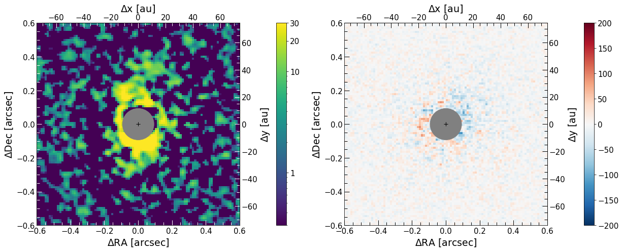
Figure 2: Left: Close up of the final $Q_{\phi}$ SPHERE/IRDIS-DPI image after removing low frequency structures (see text for details) and applying a Gaussian kernel of size 0.1 $\times$ FWHM to smooth the images and enhance the spiral features. Right: Close up of the final $U_{\phi}$ image showing the positive and negative signal. The 93 mas coronagraph is indicated by the gray circle, and the cross indicates the position of the star. The flux is normalized to the maximum value in the $Q_{\phi}$ image.

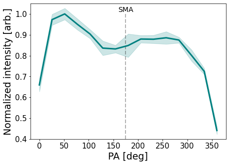
Figure 3: Azimuthal profile of the deprojected Q_ϕ image, radially averaged over a ring of 0.22-0.29” ($\sim$27 - 36 au). The two peaks at around 50^∘ and 210^∘ correspond to the launch locations of the two spiral arms. The error is taken to be 2 $\sigma$. The dashed line indicates the location of the disk’s semi-major-axis.

4.1 SPHERE/IRDIS-DPI observations

In Fig. 2 we show the final, processed $Q_{\phi}$ and $U_{\phi}$ images. Due to the low S/N, we sharpened the images by subtracting a version of them which was convolved by a Gaussian kernel with the size of 10 pixels, which removes low frequency structures, and then we convolved them with a Gaussian kernel of size 0.1 $\times$ FWHM to smooth the images in order to enhance the spiral features. We observe the launch of the spiral arms up to $\sim$0.3” (40 au), as seen in the $Q_{\phi}$ image (Fig. 2, left). As mentioned in Section 3, the $U_{\phi}$ image (Fig. 2, right) in this case contains almost no signal and can be used as an upper limit of the noise level. For a better visualization of the spiral features, we plotted the azimuthal profile by first deprojecting the filtered $Q_{\phi}$ image, and taking the average flux within the ring between $\sim$27 and 36 au in azimuthal bins of 15^∘. The distance range is chosen due to the presence of the coronagraph at lower radii, and the S/N decrease at higher radii. In Fig. 3, we show the smoothed azimuthal profile. The spiral arms are seen as the two peaks between $20^{\circ}-100^{\circ}$ and $200^{\circ}-310^{\circ}$. To estimate the spiral arm intensity contrast between the spiral and inter-spiral regions, we measured the peak intensities of the spiral arms in radial bins spaced by 2 au. We estimated the inter-spiral region intensity by taking the minimum value in each bin. The contrast is then the ratio between the peak intensities and the inter-spiral intensities. On average, we find the spiral arm contrast to be 1.5.

4.2 Companion candidate

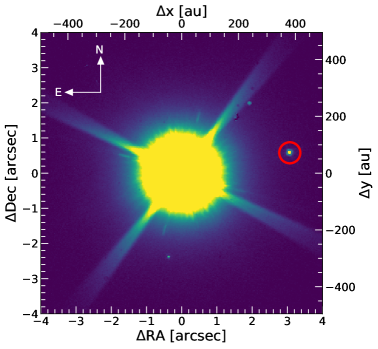
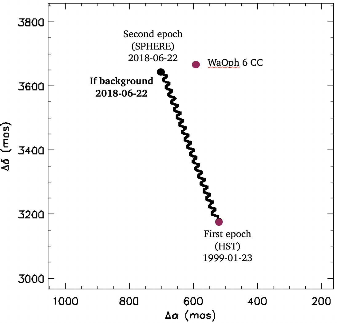
Figure 4: Top: Total intensity SPHERE/IRDIS-DPI image of WaOph 6. Encircled in red is the CC. Bottom: Astrometry plot of the CC of WaOph 6. The markers show the position of the CC, at the initial HST epoch, and further in time at the SPHERE epoch. The black curve traces the path a stationary background object would have followed relative to WaOph 6 between the two epochs.

We detect a companion candidate (CC) in our data as shown in the total intensity image in the top panel of Fig. 4, where the CC is more visible than in the polarized light frames. The CC is located at a projected distance of $\sim$400 au ($\sim$3”) and has a brightness contrast of 10^-3 with respect to WaOph 6. We used archival HST data (from 1999-01-23) as an additional epoch to perform an astrometric analysis in order to verify if the CC is bound to the system. The resulting astrometry plot is shown in the bottom panel of Fig. 4, where the black curve traces the path a stationary background object would have followed relative to WaOph 6 between the two epochs, and the markers show the position of the CC at both the HST and the SPHERE epochs. Since the CC is located near the final position a background object would be located at, we conclude that the object is not bound to the system, and therefore could not be considered as an external perturber causing the spirals. We note that the CC is not reported in the Gaia EDR3, despite of its presence in the two data sets described above.

4.3 Comparison to ALMA Observations

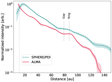
Figure 5: Radial intensity profiles of both the SPHERE and ALMA images of WaOph 6. Plotted on a logarithmic scale and normalized to the maximum intensity of each image. The SPHERE profile is taken from the reduced $Q_{\phi}$ image with an applied Gaussian kernel of size 0.1 $\times$ FWHM to smooth the curve, and it is shown up to 3$\sigma$ of the intensity. The dotted line indicates the coronagraph coverage.

WaOph 6 was observed within ALMA/DSHARP (Andrews et al., 2018) in Band 6, at a frequency of 239 GHz (1.3 mm). Observations at these wavelengths sample the millimeter-sized dust grains that are typically located in the disk midplane (see e.g., Villenave et al., 2020). On the other hand, our SPHERE observations trace the light scattered from submicron sized dust grains located at the disk surface which are typically well-coupled to the gas. In this section we do a first comparison of the two data sets.

4.3.1 Radial profiles

In Fig. 5 we plot the radial intensity profiles of the SPHERE/IRDIS-DPI H-band image (teal curve), and the ALMA image in Fig. 1 (crimson curve). The curves have been normalized to the maximum intensity value on each image for visualization purposes. In order to obtain a smooth profile, we apply a Gaussian kernel of size 0.1 $\times$ FWHM to the reduced $Q_{\phi}$ image in Appendix B. We obtained the profiles by taking the azimuthal average of the image intensity in rings of radius 3 au. For this we considered the latest literature values for $i$ and PA (listed on Table 1), and we use the aperture_photometry() function from the photutils python package, which allows to perform aperture photometry within elliptical annuli. This permits to get the radial profile without first deprojecting the image.

As expected from the fact that the two images trace different dust sizes, the profiles do not perfectly overlap. A closer look between 70 au and 90 au shows that the substructures created by the gap and the ring described in Section 2, are present in both profiles, with a slight shift. The initial drop in the intensity of the SPHERE/IRDIS-DPI profile is due to the use of a coronagraph in these observations. The cut in the ALMA data profile can be attributed to the emission from the large grains being limited to the central $\sim$130 au of the disk.

Table 3: Spiral pitch angles for the protoplanetary disk around WaOph 6.

Source	Spiral arm	Log. $\mu$ [∘]	Arch. $\mu$ [∘]
SPHERE	N	19.79${}_{-0.11}^{+0.12}$	19.54
	S	14.04${}_{-0.06}^{+0.07}$	16.05
ALMA	N1	13.49${}_{-0.19}^{+0.30}$	18.97
	S1	18.26${}_{-0.07}^{+0.04}$	15.98
	N2	10.75${}_{-0.15}^{+0.23}$	17.86
	S2	9.09${}_{-0.10}^{+0.21}$	15.26

• Note: For the SPHERE data, N corresponds to the northern spiral and S to the southern spiral. In the case of the ALMA data, N1 corresponds to the northern inner spiral, S1 to the southern inner spiral, N2 to the northern outer spiral and S2 to the southern outer spiral. For the Archimedean fit, the pitch angles are estimated at 35 au.

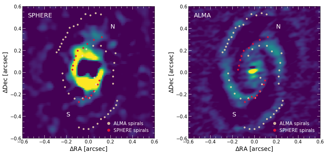
Figure 6: Left: SPHERE $Q_{\phi}$ image as described in Fig. 2 but with a Gaussian kernel of size 0.2 $\times$ FWHM with the spiral arms retrieved from both the ALMA and this image overplotted. Right: ALMA continuum image generated as described in the Appendix C, with the overplotted spiral arms retrieved from both the SPHERE $Q_{\phi}$ and this image. The “N” and “S” indicate the northern and southern spirals, respectively.

4.3.2 Spiral arms

Next, we performed a spiral search on each data set to compare the location of the spiral arms at both wavelengths. In the case of the SPHERE data, the spiral features are better seen when the image is plotted in polar coordinates, where spiral arms appear as inclined lines. To obtain the polar plot we first deprojected the image and then converted to polar coordinates. We then used the python function peak_local_max from the skimage package to search for the peak emission points around the location of the spiral arms. To trace the spirals in the ALMA data we used two different images generated using the tclean task in CASA 5.4.1 (McMullin et al., 2007). We used uv-taper = [‘0.010arcsec’, ‘0.010arcsec’, ‘10deg’], and two different robust values (-1.0 and 1.0) to generate an image with higher resolution in the central and in the outer regions, respectively. Then, we searched for peak emission points along the radial direction and took the 3$\sigma$ emission ones as the spiral arms. We repeated this process in both of the images described above. The resulting spirals are shown in Fig. 6, where we overplot the retrieved spiral arms on both the SPHERE (left) and the ALMA image (right). To obtain the SPHERE image we followed the same procedure described in Section 4 with a Gaussian kernel of size 0.2 $\times$ FWHM. We did this to match the scaling of the ALMA image for better comparison purposes. To generate the ALMA image, we used the frank (Jennings et al., 2020) tool to remove the azimuthally component of the emission of the disk and leave only the nonaxisymmetric features, as described in the Appendix C. We note that the spiral pattern is much more prominent in the mm continuum than in scattered light. Besides the low S/N of the SPHERE data and the fact that the disk has been reported to be cold, this could also be explained by the anisotropic scattering properties of the dust of different sizes. For a disk that is not edge-on, the larger the particles on the surface layer compared to the wavelength, the more they will scatter light into the disk in forward scattering. Therefore, the amount of light scattered in the line of sight direction would be smaller and would not be detected in scattered light images (e.g., Mulders et al., 2013). Additionally, we notice that there appears to be a break in the spiral arms on the ALMA image at $\sim$0.16” ($\sim$20 au), which cannot be observed in our SPHERE data. In the following we treat this break as a separate set of spirals.

In order to characterize the spirals we considered two models. A logarithmic spiral given by:

$$r=r_{0}\cdot\exp(b\theta),$$ (3)

and an Archimedean spiral, defined as:

$$r=r_{0}+b\theta,$$ (4)

where $\theta$ is the polar angle, $r_{0}$ is the radius for which $\theta$=0, and $b$ relates to the pitch angle ($\mu$) of the spiral. The pitch angle is defined as the angle between the tangents to a spiral arm and a circle drawn from the center of the disk, it describes how tightly the spiral arms are wound. In the logarithmic case, the pitch angle is constant along all radii and it is given by $\mu=\arctan(1/b)$, while for the Archimedean spiral, the pitch angle depends on the radius as $\mu=b/r$. To test the symmetry of the spiral arms, the parameters $r_{0}$ and $b$ were fitted separately, while we assumed $i$ and PA to be fixed and equal to the literature values shown in Table 1. Therefore, we had four and eight free parameters for the SPHERE and ALMA data, respectively. To fit the data, we used the MCMC code based on emcee (Foreman-Mackey et al., 2013) and described in Kurtovic et al. (2018). A flat prior probability is used for the free parameters. For each fit, we used 250 walkers with two consecutive burning stages of 1000 and 500 steps, and then 1500 steps to sample the parameter space.

The resulting pitch angles for each fit are given in Table 3, where for the SPHERE data, N corresponds to the northern spiral and S to the southern spiral; and in the case of the ALMA data, N1 corresponds to the northern inner spiral, S1 to the southern inner spiral, N2 to the northern outer spiral and S2 to the southern outer spiral. For the Archimedean fit, the pitch angles are estimated at 35 au. We find that there are some significant differences between the values of the inner and outer ALMA spirals for the logarithmic model, which leads us to conclude that the two sets might not be part of the same spiral arm. There seems to be additional structure in the region of the discontinuity, however, follow-up deeper observations would be needed to draw any conclusions of the origin of this break. Furthermore, we note that the values of the pitch angle for the corresponding spirals differ from one data set to the other, and that in the case of the Archimedean model, the scattered light pitch angles are slightly higher that those from submillimeter. This can be expected, since we are tracing different regions of the disk (the flared surface vs. the midplane). Moreover, we find that the pitch angles from the Archimedean model decrease with the distance from the star, in agreement with the results of Huang et al. (2018b).

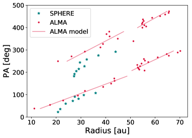
Figure 7: Polar plot showing the spiral arms of both the SPHERE (stars) and ALMA (dots) images of WaOph 6. The lines show the Archimedean best fit model for the spirals.

Figure 7 shows the spirals retrieved from both data sets in a polar map, along with the best-fit Archimedean model for each arm. We find a discontinuity in the spiral arms for the ALMA data at $\sim$50 au. This peculiarity has already been reported by Huang et al. (2018b), who also noted that this discontinuity appears to coincide with a region where there is additional bright emission between the main spiral arms, and comment that it could be explained by either the presence of a ring crossing this region, or ”spurs” emerging from the main spirals.

4.4 Origin of the spirals

Large perturbations in the disk launch sound waves that result in a spiral shape due to the differential rotation of the disk. Theoretical models have shown that such large perturbations can be driven by the presence of an embedded planetary mass perturber (e.g., Boccaletti et al., 2013), GI (e.g., Goldreich & Tremaine, 1979; Tomida et al., 2017), or a combination of both (e.g., Pohl et al., 2015).

Two-arm spirals in disks can be driven by a massive, giant planetary companion ($\gtrsim 5M_{J}$), that would typically be located at the tip of the primary arm. This scenario suggests, however, that these planets are fainter than predicted by ”hot-start” evolutionary models (Dong et al., 2018b), since the number of detections is low.

On the other hand, one criteria to test the GI hypothesis is to use the so called Toomre (1964) parameter $Q$, given by

$$\centering Q\equiv\frac{\Omega_{k}c_{\mathrm{s}}}{\pi G\Sigma},\@add@centering$$ (5)

where $\Omega_{k}$ is the angular velocity, c_s is the sound speed, and $\Sigma$ is the surface density. These parameters vary with radius in the disk, resulting in $Q$ being a function of the radius. The Toomre stability criteria states that a disk will be gravitationally stable if $Q\geq 1$ and unstable if $Q<1$.

In the case of WaOph 6, we estimated the Toomre parameter $Q$ using equation 5 and assuming $\Sigma\propto 1/\sqrt{r}$, where $r$ is the distance from the star, throughout the disk (see Appendix D for the detailed calculation) in order to see whether the disk would be stable under these conditions. We obtained that $Q$ varies from $2.2-33.2$ from the outer part of the disk inward. This indicates that the disk is fairly stable according to the Toomre stability criterion, implying that a large perturbation driving the spiral arms should have come from a source other than GI. Nonetheless, we are aware that this is not an absolute proof of GI not taking place in the disk at some earlier evolutionary state. This analysis only shows that a disk with a surface density $\propto 1/\sqrt{r}$ around a 0.98 $M_{\odot}$ star appears to be stable within our assumptions of the disk mass and the gas surface density, which should be taken with caution due to the considerable uncertainties in their calculation. In this context, we decide to test the planetary perturber hypothesis by performing hydrodynamical simulations and radiative transfer to compare with our observations.

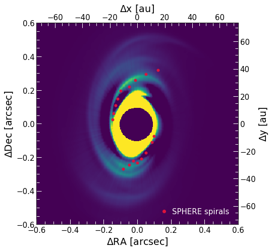
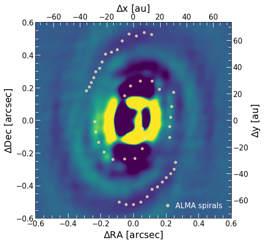
Figure 8: Radiative transfer images showing the spirals formed by a 10 M_Jup planet at 140 au. Left: Synthetic polarized scattered light $Q_{\phi}$ image with an analogous Gaussian kernel to the one applied to Fig. 6, left. The dark central area shows the coronagraph coverage. Right: Synthetic mm continuum image after subtracting the azimuthal average flux on the image plane to enhance the spirals, analogous to the procedure applied to Fig. 6, right. The red and white dots denote the location of the observed spirals for each image, respectively.

5 Modeling

In order to test the hypothesis of a forming planet causing the spiral features, we performed 3D gas-only and 2D gas+dust hydrodynamical simulations in which a massive planet at a separations $\geq 90$ au generates large-scale spiral arms interior to its orbit. To compare the results to our observations, we fed the resulting density distributions into a radiative transfer code to generate synthetic images.

5.1 Hydrodynamical models

To model the dust on the surface sampled by scattered light, we ran 3D simulations of the gas dynamics using the hydrodynamical code PLUTO (Mignone et al., 2007). The gas distribution was initially set following a vertically isothermal configuration at hydrostatic equilibrium (see, e.g., Fromang et al., 2011). The disk temperature depends on the cylindrical radius $R$ from the center of the domain as $T\propto R^{-1/2}$, whereas the gas pressure scale height is computed as $H=c_{s}/\Omega_{K}$, where $c_{s}\propto T^{1/2}$ is the local sound speed and $\Omega_{K}\propto R^{-3/2}$ is the Keplerian angular velocity. With the chosen parameters, the disk aspect ratio depends on $R$ as $H/R\propto R^{1/4}$, with $H/R=0.1$ at $R=50$ au. The gas volumetric density decreases with $R$ as $\rho\propto R^{-7/4}$, in such a way that the surface density varies as $\Sigma\approx\sqrt{2\pi}H\rho\propto R^{-1/2}$. A locally isothermal equation of state is applied such that the initial temperature distribution is maintained through time.

The hydrodynamical equations were solved in spherical coordinates in a reference frame centered at the star-planet center of mass corotating with the system. The computational domain, given by the region $(r,\theta,\phi)\in[8,210]\,\mathrm{au}\times[\pi/2-0.3,\pi/2+0.3]\times[0,2\pi]$, is discretized using a grid of resolution $N_{r}\times N_{\theta}\times N_{\phi}=256\times 64\times 512$ logarithmically spaced in the $r$-direction and uniformly spaced in the remaining ones. All computed fields are fixed to their initial values at the radial boundaries except for the density and the radial velocity, which are reflected and extrapolated in the ghost zones, respectively. On the vertical boundaries, reflective conditions are applied. The gravitational potential is computed as the sum of the potentials of the star and the planet. To avoid divergences, the later is modified in the vicinity of the planet location following the prescription by Klahr & Kley (2006), employing a smoothing length equal to half the planet’s Hill radius. For stability purposes, the planet mass is smoothly increased from $0$ to its final value in a total time of $100$ yr. We also included viscosity with constant $\alpha=10^{-3}$. The resulting dust mass distribution was computed assuming a perfect coupling between the dust particles and the gas flow, with a uniform dust-to-gas mass ratio of $10^{-2}$.

To model the dust evolution in the midplane sampled mainly by the millimeter observations, we ran two-dimensional hydrodynamical simulations using the multi-fluid version of the code FARGO3D (Benítez-Llambay & Masset, 2016; Benítez-Llambay et al., 2019). It solves the Navier-Stokes equations of the gas and multiple dust species, each one modeled as a pressureless fluid that represents a specific grain size. We traced eight different dust species in our simulations. The initial gas temperature, gas surface density structure, equation of state and gas viscosity prescription of the 2D model are equivalent to our 3D simulations model, described above. The initial dust surface density in our simulation has the same structure as the gas surface density, while set by an initial dust-to-gas mass ratio of $10^{-2}$ everywhere in the disk. We traced the dynamical evolution of eight dust fluids, that are logarithmically spaced in size, and followed a dust size distribution $n(s)\propto s^{-2.5}$ with minimum and maximum dust sizes of $10\,\rm\mu m$ and $100\,\rm\mu m$. We set the dust intrinsic density to $2.0\,\rm g\,cm^{-3}$. The dynamics of the dust fluids is dictated by its local Stokes number (dimensionless stopping time), defined as $\mathrm{St}=\pi a_{i}\rho_{int}/2\Sigma_{g}$, where $a_{i}$ is the grain size of the size-bin, $\rho_{int}$ the intrinsic grain density and $\Sigma_{g}$ the gas surface density. Dust diffusion was included in the simulation following the same prescriptions implemented in Weber et al. (2019), which are based on the results of Youdin & Lithwick (2007). Dust feedback onto the gas, dust growth, and dust fragmentation were not included in our simulations. The two-dimensional grid is linear in azimuth and logarithmic in radius, using 512 cells in $\phi$ covering $2\pi$, and 256 cells in $r$ covering from $\sim 8.4$ au to $\sim 420$ au. A planet was slowly introduced over $\leavevmode\nobreak\ 8\times 10^{4}$ yr fixed at the given radius, driving spiral density waves in the disk. The planet’s potential was smoothed by a length factor of 60% the disk scale height. For a more detailed description of the FARGO3D multi-fluid simulations see also Weber et al. (2019). Our test runs show that only dust fairly well coupled to the gas follows the spiral density waves (as shown by e.g., Veronesi et al., 2019; Sturm et al., 2020), with Stokes numbers below $\sim 10^{-2}$. Dust particles with larger Stokes number decouple from the gas and form axisymmetric rings. Fixing the disk gas surface density given the mass constraint from the observations, and the dust intrinsic density to a standard value, limiting the maximum dust size to $100\,\rm\mu m$ in our models is required to maintain the Stokes number of the dust observed at millimeter wavelengths below $\sim 10^{-2}$, therefore, the simulated dust particles trace the spiral arm structure. A summary of the parameters used in our simulations can be found in Table 4.

Table 4: Summary of simulations parameters.

Parameter	2D gas+dust	3D gas
Aspect Ratio at 100 au	0.12	0.12
Flaring Index	0.25	0.25
Surface Density Slope	0.5	0.5
Alpha Viscosity	$10^{-3}$	$10^{-3}$
Stellar Mass	0.98 $M_{\odot}$	0.98 $M_{\odot}$
Planet-to-Star Mass Ratio	$10^{-2}$	$10^{-2}$
Planet Orbital Radius	140 au	140 au
$\#$ of Cells in $r$	256	256
$\#$ of Cells in $\phi$	512	512
$\#$ of Cells in ${\theta}$	-	64
Grid Inner Radius	8.4 au	8 au
Grid Outer Radius	420 au	210 au
Total Evolution Time	$4\times 10^{5}$   $\mathrm{yr}$	$4\times 10^{5}$  $\mathrm{yr}$
Dust-to-Gas Mass Ratio	10-2	-
Maximum Dust Size	100 $\mu$m	-
Minimum Dust Size	10 $\mu$m	-
Dust Size Slope	2.5	-
Dust Intrinsic Density	2.0 g cm-3	-

We sample the parameter space of a planet with masses between $2-15$ M_Jup and separations between $90-160$ au (see Appendix E, Fig. 11 for some of the resulting density maps). The lower limit in the mass range is chosen based on the results of Juhász et al. (2015), who concluded that observable spiral arms are formed for planets with M $>1\mathrm{M}_{\mathrm{Jup}}$. Tighter constraints on the lower limit of the planet mass can be obtained from spiral arm formation theory. For a planet with a mass larger than three thermal masses (M${}_{th}\equiv c_{s}^{3}/\Omega G=\mathrm{M}_{\star}(h/r)_{p}^{3}$), two spiral arms will form interior to its orbit (Bae & Zhu, 2018). Since we wanted to model $m=2$ spirals, we chose to place the planets outside of the spiral arm (which extends up to 90 au in the millimeter continuum) based on the results of Dong et al. (2015). Assuming that the planet is outside $\sim$ 90 au and the disk aspect ratio of our model, we obtained that two spirals are formed for planet masses larger than $\sim$ 4.8 $M_{\mathrm{Jup}}$. Another criteria for the planet mass comes from the separation between the primary and secondary spiral arms ($\phi_{sep}$). Fung & Dong (2015) obtained that this quantity scales with the planet mass, following $\phi_{sep}=102^{\circ}(q/0.001)^{0.2}$, where in this case $q$ is the planet-to-star mass ratio. If we consider that the spiral arms have a separation range between $135^{\circ}$ and $180^{\circ}$, we obtain that the planet mass should be between 4 and 17 $M_{\mathrm{Jup}}$. After a few test runs in our simulations, we realized that in order to observe the disk truncate at 90 au (consistent with the disk outer edge in the millimeter continuum), when increasing the separation, we should also increase the planet mass. Snapshots of the gas and total dust surface densities of our 3D and 2D hydro simulations for planets of 5, 10 and 15 M_Jup at separations of 130, 140 and 160 au, respectively, are shown in the Appendix E.

5.2 Radiative transfer

In order to compare the results generated by the procedure described in the last section with our observations, we generated images in both polarized NIR and millimeter continuum using the radiative transfer code RADMC-3D (Dullemond et al., 2012). We obtained synthetic scattered light images using the dust mass distribution computed in the described 3D PLUTO simulations. Based on Ricci et al. (2010), we assumed a dust size distribution $n(s)\propto s^{-2.5}$ and model scattering by submicron particles with sizes ranging between $0.01$ and $0.5$ $\mu$m. To compute the dust mass in this range, we used the total dust mass estimated in this work (see Table 1) assuming maximum grain sizes in the mm, to obtain M${}_{\mathrm{dust,<0.5\,\mu\mathrm{m}}}=10^{-9}$ M_⊙. Opacities are computed assuming a dust composition of $60\%$ astronomical silicates and $40\%$ amorphous carbon grains, taking the optical constants respectively from Draine & Lee (1984) and Li & Greenberg (1997), and combining them following the Bruggeman mixing rule. Scattering matrices were computed assuming spherical dust grains using the BHMIE code (Bohren & Huffman, 1983) for Mie scattering. For the scattered light computations, we approximated the grain size distribution using $5$ size bins. To smooth out oscillations in the polarization degree occurring when considering spheres of a single size (see, e.g., Keppler et al., 2018), we used a Gaussian size distribution within each bin with a FWHM of $20\%$ of the corresponding grain size. The star was modeled as a point source located at the domain center emitting thermal radiation with characteristics summarized in Table 1. We used RADMC-3D to model anisotropic scattering with full treatment of polarization, using a total of $10^{8}$ photon packages. The obtained Stokes $Q$ and $U$ frames were then convolved by a Gaussian PSF with a FWHM of $51$ mas to reproduce the resolution of the VLT/SPHERE observations (see Section 3), after which we used equation (2) to obtain the resulting $Q_{\phi}$ images.

To compare with the ALMA data, we computed radiative transfer predictions of the dust continuum, in this case, using the output of the dust and gas 2D simulation. We used the dust density field from the simulation as input for RADMC-3D. We expanded the two-dimensional surface density vertically, assuming a Gaussian shape, where the volumetric mass density for each dust bin follows:

$$\rho_{i}(r)=\frac{\Sigma_{i}(r)}{\sqrt{2\pi}H_{i}(r)}\times\exp\left(-\frac{z^{2}}{2H_{i}^{2}}\right),$$ (6)

where $H_{i}$ indicates the pressure scale height of the dust bin. The vertical settling of the disk follows a standard diffusion model (Dubrulle et al., 1995):

$$H_{i}=\sqrt{\frac{\tilde{\alpha}}{\tilde{\alpha}+St_{i}}}H_{g},$$ (7)

where $H_{g}$ is the gas pressure scale height, $St$ is the dust Stokes number, and $\tilde{\alpha}=\alpha/Sc_{z}$ with $\alpha$ the $\alpha$-viscosity value of the gas. $Sc_{z}$ is the Schmidt-number, set to 1 $Sc_{z}$ relates the dust diffusion coefficient with the gas viscosity $D_{z}=\nu/Sc_{z}$ (see also Weber et al. (2019)). We used optool to compute the dust asorption and scattering opacities of a mixture using standard Mie theory and Bruggeman rules. We assumed that the composition of the dust grains is a mixture of silicates (internal density of 3.2 g/cm³), amorphous carbon (internal density of 2.3 g/cm³), and vacuum. Assuming that the solids in the mixture are 60% silicates and 40% carbon, a volume fraction of 25% of vacuum in the mixture is required so its internal density is $\sim 2$ g/cm³. The dust size distribution is equal to the values used for the simulation, set by the power law $n(s)\propto s^{-2.5}$, with maximum and minimum dust sizes of 100 $\mu$m and 10 $\mu$m, respectively. The total dust mass in our models is $\sim 10^{-4}\,\mathrm{M}_{\odot}$. We computed the dust temperature using the Monte Carlo method of Bjorkman & Wood (2001), and the continuum emission image via ray-tracing, taking into account absorption and scattering, assuming Henyey–Greenstein anisotropic scattering. We computed simulated ALMA observations from the radiative transfer synthetic continuum image using CASA (version 5.6) simobserve and tclean tasks. Following the observations setup from the DSHARP survey (Andrews et al., 2018), we simulated an 8 h integration in configuration C43-8 combined with a 15 min integration in C43-5. Finally, we cleaned the image using briggs weighting 1.0. We obtained a beam size of $55\times 53$ mas and PA of $\sim-55^{\circ}$, directly comparable to the ALMA observation.

5.3 Results and comparison to observations

All tested planets drive $m=2$ spiral arms whose symmetry increases for larger planetary mass and have a low contrast in the dust surface density (as seen in the density plots shown in Fig. 11). Given the asymmetry in the $5$ M_Jup case, we conclude that in case the spirals are caused by a planet, its mass should be at least of approximately $10$ M_Jup. In Fig. 8 we show resulting radiative transfer images for a 10 M_Jup planet at a separation of 140 au, with spiral arms observable both in the scattered light and millimeter continuum observations. For a better comparison to the simulations, we apply a Gaussian kernel to the image on the left panel, similar to the one used for the SPHERE image in Fig. 6, left; and we subtract the azimuthal average flux on the image plane to enhance the spirals on the synthetic millimeter continuum image on the right, analogous to the procedure applied to Fig. 6, right. Additionally, we overplot the location of the observed spiral arms. The obtained images resemble the ones detected both in the scattered light and millimeter continuum observations, except for the fact that we are only able to fit either the inner or the outer spirals from the millimeter observations, but not both at the same time (see Fig. 12, lower panel). This is likely due to missing physics in our simulations, as these models of spirals launched by a single planet are unable to reproduce the break in the spirals observed by ALMA, as well as the gap and the ring features (at 79 and 88 au, respectively) in the observations. We must also note that in order to see spiral arms induced by a planet in millimeter continuum, the dust must be fragmentation limited (e.g., Birnstiel et al., 2010) leading to a small dust maximum size, and therefore, to Stokes numbers small enough to follow the spirals. In protoplanetary disks, the maximum grain size is mainly set by radial drift or fragmentation of particles after collisions. The later depends on the disk viscosity and the threshold considered for the fragmentation velocity of the grains. Assuming low fragmentation velocities for ice grains (e.g., $<$ 1 m/s, as suggested by recent laboratory experiments such as Musiolik & Wurm, 2019; Steinpilz et al., 2019), and alpha=$10^{-}3$ (as taken in the simulations), the maximum grain size in the entire disk is dominated by fragmentation, limiting the maximum size of  100$\mu$m (Pinilla et al., 2021). Kataoka et al. (2016) have found that dust with similar characteristics is traced by millimeter continuum observations of the similarly young disk HL Tau. These characteristics are not required to see spirals generated by GI, where the dust trapping in spirals is efficient for larger dust Stokes numbers (Rice et al., 2004). We also note that none of the parameter sets that we sample are able to reproduce the contrast nor the apparent break in the spiral arms shown in the ALMA data, which might be explained by additional physical processes occurring in the disk. However, more complex simulations including other effects (e.g., dust growth, fragmentation, dust feedback, gas temperature evolution) are beyond the scope of this work. Additionally, we note that a planet of 10 M_Jup in such a young disk could have either formed via gravitational collapse when the disk was probably more massive and, therefore, gravitationally unstable (Boss, 1997), or formed as a stellar companion from cloud fragmentation due to the planet/star mass ratio ($\sim$1%, Reggiani et al., 2016). We would like to mention that this is a first attempt to find a plausible planetary model to explain the observed spiral pattern in the protoplanetary disk around WaOph 6 and that further, deeper observations would be needed to confirm or discard this scenario.

Since we employ an isothermal equation of state, the spirals produced in our simulations are induced solely by Lindblad resonances and not by buoyancy modes, which may be triggered when using finite cooling times. It is argued in Bae et al. (2021) that such modes cannot be observed in millimeter continuum observations, but could potentially be seen in scattered light. The pitch angles for buoyancy resonances shown in that work for up to 2 M_Jup planets are generally below those seen in our SPHERE observations (see Table 3), which suggests that the observed spirals are likely not triggered by such modes. Future resolved CO line emission observations analyzing the disk kinematic structure could help discard or verify this hypothesis (Bae et al., 2021).

6 Discussion

6.1 Observations in NIR and mm

Our SPHERE/IRDIS-DPI observations show the launch of an $m=2$ spiral pattern in the disk around WaOph 6. This is a surprising finding, since so far, no spiral arms had been observed in scattered light in disks around K and/or M stars with ages $<1$ Myr. Moreover, spiral arms have not been observed at these wavelengths in single T Tauri stars of any age (Garufi et al., 2018). Disks with spiral arms detected in scattered light are thought to be older (with the caveat that stellar ages are highly uncertain), and with stellar hosts of spectral types from G to A (e.g., MWC 758, Dong et al. (2018a), HD 142527, Claudi et al. (2019), HD 100546, Pérez et al. (2020), AB Aur, Boccaletti et al. (2020), HD 100453, Benisty et al. (2017)). In the millimeter continuum, most of these disks show asymmetric morphologies, along with large cavities (e.g., Tang et al., 2017; Cazzoletti et al., 2018; Pineda et al., 2019). Further observations in both scattered light and millimeter continuum of K and M type stars with disks would be needed to determine whether spiral arms are a common feature in such young disks, as well as the possible implications that this might have in dust and gas evolutionary models. We also note that comparing observations at different wavelengths can contribute greatly to the understanding of the physical processes driving the different morphologies seen in protoplanetary disks.

From our hydrodynamical simulations, we observe that in order to obtain a spiral pattern that can be observed in the millimeter continuum data, the dust particles must have a limited maximum size. This has previously been observed in dust evolution simulations by Gerbig et al. (2019), and can be linked to the young age of the disk.

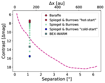
Figure 9: Planet detection limits as a function of the separation from the star for the SPHERE H-band. The purple curve is the $3\sigma$ contrast obtained from the total intensity SPHERE image of WaOph 6. The markers show the magnitude contrast of the proposed 10 M_Jup planet at 140 au estimated from different evolutionary models. The red markers show the resulting contrast for the “hot-start” scenario from the Baraffe et al. (2003) (red diamond) and Spiegel & Burrows (2012) (red dot) models, while the blue dot shows the contrast for a “cold-start” from the Spiegel & Burrows (2012) models. The green square shows the contrast from the BEX-WARM models (see text). And the green dots show the contrast for different initial entropy values from the Spiegel & Burrows (2012) models.

6.2 Upper limits on the brightness of point sources

We used the total intensity image derived from our SPHERE/IRDIS-DPI observations to obtain information on the detection limits for WaOph 6. We built the contrast curve in Fig. 9 by considering the contrast between WaOph 6 (the central brightest pixel) and a representative planetary signal in the total intensity image. We took the planetary signal to be three times the noise (root mean square) in 2 pixel wide annuli centered on the star, at different separations up to $\sim$6” ($\sim$740 au). Additionally, we estimated the foreground extinction in the H-band toward WaOph 6. For this we first estimated the reddening by using the intrinsic $J-H$ magnitude of a K6V star from Pecaut & Mamajek (2013), then using the values in Table 3 of Rieke & Lebofsky (1985), we obtained a visual extinction of $A_{V}=5.08$ mag, and an H-band extinction of $A_{H}=0.88$ mag.

To estimate the apparent magnitude of our proposed planet, we used two independent evolutionary model predictions. On one hand we considered the evolutionary models by Baraffe et al. (2003) for a 10 M_Jup planet at 1 Myr. On the other hand, we used the evolutionary models proposed by Spiegel & Burrows (2012) for both a “hot” and “cold-start” scenarios, and we extrapolated the H-band absolute magnitude (M_H) for our 10 M_Jup planet at 0.7 Myr. Considering extinction toward WaOph 6, we obtain $\mathrm{m}_{H}=15.26$ mag, $\mathrm{m}_{H}=14.91$ mag, and $\mathrm{m}_{H}=23.07$ mag, respectively for each model. Finally, with the H-band magnitude for WaOph 6, $\mathrm{m}_{H}=7.57$ mag, we obtained the following contrasts: $\Delta$mag$=7.70$, $\Delta$mag$=7.36$, and $\Delta$mag$=15.49$ mag, respectively. Furthermore, we obtained the contrasts for our proposed planet in the “warm-start” scenario from the initial entropy values reported by Spiegel & Burrows (2012). And as an additional comparison, we used the Bern EXoplanet cooling curves (BEX, Mordasini et al., 2017) coupled with the COND atmospheric models (Allard et al., 2001) reproducing the cooling under “warm-start” initial conditions (Marleau et al., 2019), and thus denominated BEX-WARM model (see Asensio-Torres et al., 2021, and references therein for more details). As seen in Fig. 9, the detectability of our proposed planet strongly depends on the adopted formation model. In case of the “hot-start” scenario, the planet should have been observed, while for a large part of the “warm-start” and for the “cold-start” scenarios, the planet contrast is below our detection limits. Based on the planet mass and location, a “warm” to “cold” start model would be more plausible to explain its existence.

Additional detection limits for WaOph 6 in the L’-band ($\lambda_{0}=3.8\,\mu$m) have been recently reported by Jorquera et al. (2020). They do not detect any companion candidates to the star, but report detection probability maps obtained using the (Baraffe et al., 2003) models. From these they preliminary rule out the presence of companions with masses $>5$ M_Jup at separations $>100$ au. However, they advise that these estimates might be optimistic, since they do not consider extinction effects, either toward WaOph 6, nor due to the disk dust. An additional caveat comes from the models, as they become very uncertain in accurately predicting the properties of very young planets. It is also important to note that our hydrodynamical simulations do not include additional physical processes that could be ongoing in the disk, coming from the fact that spiral arm formation by a planetary mass object is still not well understood. This could lead to an overestimation of the planet mass, which along with evolutionary models uncertainties, could explain our differing results.

7 Summary and conclusions

We have presented for the first time scattered light SPHERE/IRDIS-DPI observations of the disk around WaOph 6 in the H-band. We analyzed the disk morphology, and used archival ALMA data to compare with ours. We tested the planetary mass perturber hypothesis as the underlying cause for the spiral structure by performing hydrodynamical simulations and using radiative transfer. Our results are summarized below:

1. We observe the launch of a set of $m=2$ spiral arms up to $\sim$0.3” (40 au) in our $Q_{\phi}$ SPHERE/IRDIS-DPI images as seen in Fig. 2, left. These spirals were first detected using millimeter continuum observations from the ALMA/DSHARP survey. To our knowledge, WaOph 6 is the youngest disk to show spiral features in scattered light (Garufi et al., 2018). We note that this might be of interest for dust and gas evolutionary models.
   

2. We observe a companion candidate at about 3” from the star in our data, as shown in the top panel of Fig. 4. After the astrometric analysis described in Section 4.2, we were able to determine that the CC is not bound to WaOph 6. With this we also discard the CC being a possible cause of the spiral structure.
   

3. Comparing our SPHERE observations with archival ALMA/DSHARP data, we find that both the gap and the ring features at 79 and 88 au, respectively, seem to be present in both data sets. We traced the spiral features in both observations as seen in Fig. 6. For the ALMA data, we notice a break in the spiral arms of the ALMA image at $\sim$0.16” ($\sim$20 au), which is not observed in our SPHERE data. We treated this break as a separate set of spirals, however, its origin remains unknown. When plotting the spirals in polar coordinates (Fig. 7) we find a discontinuity in the spiral arms for the ALMA data at $\sim$50 au, already reported by Huang et al. (2018b).
   

4. To test the planetary mass perturber hypothesis we performed hydrodynamical simulations combined with radiative transfer to compare with the observations. We tested the parameter space of a planet with masses between $2-15$ $\mathrm{M}_{\rm{Jup}}$ and separations between $90-160$ au (i.e., outside of the spiral structure). All tested planets drive $m=2$ spiral arms. However, none of the parameter sets that we sample are able to reproduce the contrast nor the apparent break in the spiral arms shown in the ALMA data, which may be due to additional physical processes occurring in the disk. Furthermore, the tested planets do not reproduce the gap nor the ring features at 79 and 88 au, respectively, these features need further investigation outside the scope of this work. Given the symmetry of the observed spirals, we find that, if these are caused by a planet, its mass is likely of at least 10 M_Jup. This is a first attempt to explain the spiral structure seen in both data sets, and more data are needed to better constrain the underlying cause of the spiral features.
   

5. To determine the sensitivity of our data to possible companions embedded in the disk, we generated the contrast curve in Fig. 9 from the total intensity image. With this we obtain contrast limits for a planetary/substellar companion forming inside the disk in polarized light. We estimate the contrast of our proposed planet using different evolutionary models, where the possibility of detection strongly depends on the formation scenario. A “warm” to “cold” starts would explain the nondetection of the planet in our SPHERE data.

In conclusion, the findings in this work highlight the still unknown complexity of WaOph 6. The striking presence of a spiral pattern in scattered light even in limited S/N data are worth further, deeper observations of this source. Which will additionally serve to confirm or discard a planetary perturber as a possible cause behind the spiral features.

Appendix A Dust mass estimate

Millimeter continuum observations, obtained assuming optically thin emission (Hildebrand 1983), allow us to use the relation

$$\centering M_{\mathrm{dust}}\simeq\frac{d^{2}F_{\nu}}{\kappa_{\nu}B_{\nu}(T(r))},\@add@centering$$ (8)

where $d$ is the distance to the star; $F_{\nu}$ is the total flux at a given frequency $\nu$; $\kappa_{\nu}$ is the dust opacity at a given frequency, for which we used the common relation applied to disk surveys, $\kappa_{\nu}$ = 2.3 $\mathrm{cm^{2}g^{-1}}\times$ ($\nu$/230 GHz)^0.4 (Andrews et al. 2013); and $B_{\nu}(T_{\mathrm{dust}})$ is the Planck function for a given dust temperature $T_{\mathrm{dust}}$, that we derived from the relation

$$\centering T_{\mathrm{dust}}=22\times(L_{*}/L_{\astrosun})^{0.16}K,\@add@centering$$ (9)

from van der Plas et al. (2016), which gives $T_{\mathrm{dust}}=$ 26.05 K. The resulting dust mass from equation 8 is reported in Table 1, and, assuming a dust/gas mass ratio ($M_{\mathrm{dust}}/M_{\mathrm{gas}}$) of 1:100, within the previously reported values. However, we are aware that the assumptions made to perform this calculation could significantly differ from the actual disk conditions and therefore, this result should be taken with caution.

Appendix B Unprocessed reduced $Q_{\phi}$ and $U_{\phi}$ SPHERE images

Figure 10 shows the reduced $Q_{\phi}$ and $U_{\phi}$ images (on the left and right panels, respectively). The raw data was reduced as detailed in Section 3. Most of the signal is concentrated in the $Q_{\phi}$ image. Due to the low S/N, these images had to be processed for the analysis as described in Section 4.1.

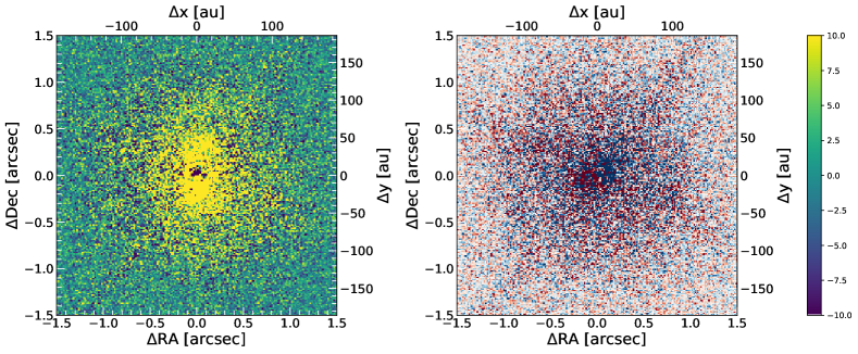
Figure 10: Reduced $Q_{\phi}$ and $U_{\phi}$ SPHERE/IRDIS-DPI images. The images are shown up to the distance where the noise dominates. Most of the signal is contained in the $Q_{\phi}$ image.

Appendix C On extracting the nonaxisymmetric information from the ALMA data

To recover the millimeter spiral structure, we follow a similar procedure to the one described in the Appendix B of Isella et al. (2019). We start from the calibrated visibilities of the dust continuum emission, available from the DSHARP data release. We run a MCMC (Monte Carlo Markov Chain) with 50 walkers to find the offset ($\delta$ RA, $\delta$ Dec) that minimizes the imaginary part of the visibilities, this gives us the centroid of the disk. In this MCMC we use a flat prior over both dimensions. After correcting by that center, we use the inclination and position angle measured by Huang et al. (2018a) to deproject the visibilities. Our new deprojected data set is analyzed with frank (Jennings et al. 2020), and the best visibilities profile found by this package is substracted from our deprojected data set. The result is a visibility set which only contains the nonaxisymmetric information of the disk, shown in the right panel of Figure 6.

Appendix D Toomre parameter calculation

From equation 5, we take

$$\centering\Omega_{k}=(GM_{*}/r^{3})^{1/2},\@add@centering$$

$$\centering c_{s}=h\Omega_{k},\@add@centering$$

where $h\propto r^{5/4}$, and

$$\centering\Sigma=\Sigma_{0}r^{-1/2},\@add@centering$$

where

$$\centering\Sigma_{0}=\frac{3M_{\mathrm{disk}}}{4\pi}\frac{1}{r_{\mathrm{max}}^{3/2}-r_{\mathrm{min}}^{3/2}},\@add@centering$$

which finally leads to $Q\propto r^{-5/4}$. We use $r_{\mathrm{min}}=20$ au due to the inner working angle limit of the observations, and $r_{\mathrm{max}}=175$ au as the outer radius from the lower limit value used by Ricci et al. (2010), the only difference when taking the upper limit is that the disk becomes unstable by $\sim$ 330 au.

Appendix E Gallery of density distributions from the hydrodynamical simulations and radiative transfer images

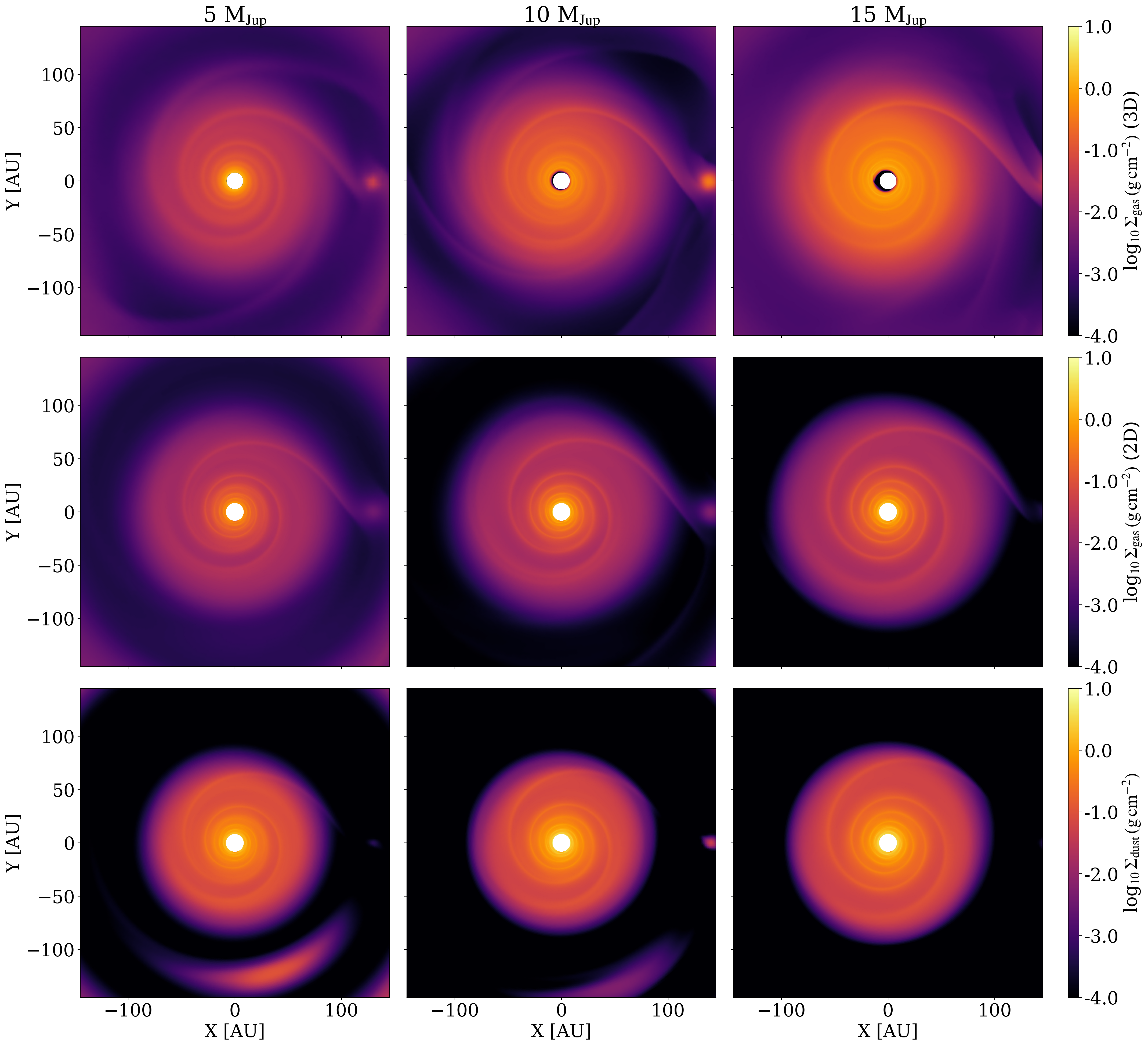
Figure 11: Density maps from our 3D (top panels) and 2D (middle and bottom panels) hydrodynamical simulations for planets of 5, 10 and 15 M_Jup at separations of 130, 140 and 160 au, respectively, shown from left to right. The top and middle panels show the gas surface density maps, while the bottom panels show the dust density maps.

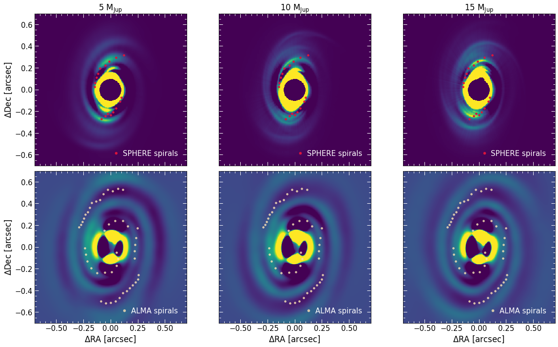
Figure 12: Resulting radiative transfer images from our 3D (upper panels) and 2D (lower panels) hydrodynamical simulations for the planets described in Fig. 11. The mass and separation increase from left to right. The images have been processed with the same techniques as the ones in Fig. 8 for a better comparison to the observations. For the lower panels, we show the images that fit the inner spirals.

Density maps from our 3D gas and 2D gas $+$ dust hydrodynamical simulations for a planet of 5, 10 and 15 M_Jup at separations of 130, 140 and 160 au, respectively are shown in Fig. 11. The resulting radiative transfer images from these simulations are shown in Fig. 12. For the case of the synthetic ALMA images, our simulations do not fit the inner and outer spirals at the same time (see Section 5.3), we show the ones fitting the inner spirals.

References

- Allard et al. (2001) Allard, F., Hauschildt, P. H., Alexander, D. R., Tamanai, A., & Schweitzer, A. 2001, ApJ, 556, 357
- Andrews (2020) Andrews, S. M. 2020, ARA&A, 58, 483
- Andrews et al. (2018) Andrews, S. M., Huang, J., Pérez, L. M., et al. 2018, ApJ, 869, L41
- Andrews et al. (2013) Andrews, S. M., Rosenfeld, K. A., Kraus, A. L., & Wilner, D. J. 2013, ApJ, 771, 129
- Andrews & Williams (2007) Andrews, S. M. & Williams, J. P. 2007, ApJ, 671, 1800
- Andrews et al. (2009) Andrews, S. M., Wilner, D. J., Hughes, A. M., Qi, C., & Dullemond, C. P. 2009, ApJ, 700, 1502
- Asensio-Torres et al. (2021) Asensio-Torres, R., Henning, T., Cantalloube, F., et al. 2021, arXiv e-prints, arXiv:2103.05377
- Avenhaus et al. (2018) Avenhaus, H., Quanz, S. P., Garufi, A., et al. 2018, ApJ, 863, 44
- Bae et al. (2021) Bae, J., Teague, R., & Zhu, Z. 2021, ApJ, 912, 56
- Bae & Zhu (2018) Bae, J. & Zhu, Z. 2018, ApJ, 859, 118
- Baraffe et al. (2003) Baraffe, I., Chabrier, G., Barman, T. S., Allard, F., & Hauschildt, P. H. 2003, A&A, 402, 701
- Baraffe et al. (2015) Baraffe, I., Homeier, D., Allard, F., & Chabrier, G. 2015, A&A, 577, A42
- Benisty et al. (2015) Benisty, M., Juhasz, A., Boccaletti, A., et al. 2015, A&A, 578, L6
- Benisty et al. (2017) Benisty, M., Stolker, T., Pohl, A., et al. 2017, A&A, 597, A42
- Benítez-Llambay et al. (2019) Benítez-Llambay, P., Krapp, L., & Pessah, M. E. 2019, ApJS, 241, 25
- Benítez-Llambay & Masset (2016) Benítez-Llambay, P. & Masset, F. S. 2016, ApJS, 223, 11
- Beuzit et al. (2019) Beuzit, J. L., Vigan, A., Mouillet, D., et al. 2019, A&A, 631, A155
- Birnstiel et al. (2010) Birnstiel, T., Ricci, L., Trotta, F., et al. 2010, A&A, 516, L14
- Bjorkman & Wood (2001) Bjorkman, J. E. & Wood, K. 2001, ApJ, 554, 615
- Boccaletti et al. (2020) Boccaletti, A., Di Folco, E., Pantin, E., et al. 2020, A&A, 637, L5
- Boccaletti et al. (2013) Boccaletti, A., Pantin, E., Lagrange, A. M., et al. 2013, A&A, 560, A20
- Bohren & Huffman (1983) Bohren, C. F. & Huffman, D. R. 1983, Absorption and scattering of light by small particles
- Boss (1997) Boss, A. P. 1997, Science, 276, 1836
- Bressan et al. (2012) Bressan, A., Marigo, P., Girardi, L., et al. 2012, MNRAS, 427, 127
- Calcino et al. (2020) Calcino, J., Christiaens, V., Price, D. J., et al. 2020, MNRAS, 498, 639
- Carbillet et al. (2011) Carbillet, M., Bendjoya, P., Abe, L., et al. 2011, Experimental Astronomy, 30, 39
- Cazzoletti et al. (2018) Cazzoletti, P., van Dishoeck, E. F., Pinilla, P., et al. 2018, A&A, 619, A161
- Chauvin et al. (2017) Chauvin, G., Desidera, S., Lagrange, A. M., et al. 2017, in SF2A-2017: Proceedings of the Annual meeting of the French Society of Astronomy and Astrophysics, ed. C. Reylé, P. Di Matteo, F. Herpin, E. Lagadec, A. Lançon, Z. Meliani, & F. Royer, Di
- Choi et al. (2016) Choi, J., Dotter, A., Conroy, C., et al. 2016, ApJ, 823, 102
- Cieza et al. (2020) Cieza, L. A., González-Ruilova, C., Hales, A. S., et al. 2020, MNRAS[arXiv:2012.00189]
- Claudi et al. (2019) Claudi, R., Maire, A. L., Mesa, D., et al. 2019, A&A, 622, A96
- Cuello et al. (2019) Cuello, N., Dipierro, G., Mentiplay, D., et al. 2019, MNRAS, 483, 4114
- de Boer et al. (2020) de Boer, J., Langlois, M., van Holstein, R. G., et al. 2020, A&A, 633, A63
- Dipierro et al. (2015) Dipierro, G., Pinilla, P., Lodato, G., & Testi, L. 2015, MNRAS, 451, 974
- Dong et al. (2018a) Dong, R., Liu, S.-y., Eisner, J., et al. 2018a, ApJ, 860, 124
- Dong et al. (2018b) Dong, R., Najita, J. R., & Brittain, S. 2018b, ApJ, 862, 103
- Dong et al. (2015) Dong, R., Zhu, Z., Rafikov, R. R., & Stone, J. M. 2015, ApJ, 809, L5
- Draine & Lee (1984) Draine, B. T. & Lee, H. M. 1984, ApJ, 285, 89
- Dubrulle et al. (1995) Dubrulle, B., Morfill, G., & Sterzik, M. 1995, Icarus, 114, 237
- Dullemond et al. (2012) Dullemond, C. P., Juhasz, A., Pohl, A., et al. 2012, RADMC-3D: A multi-purpose radiative transfer tool
- Eisner et al. (2005) Eisner, J. A., Hillenbrand, L. A., White, R. J., Akeson, R. L., & Sargent, A. I. 2005, ApJ, 623, 952
- Foreman-Mackey et al. (2013) Foreman-Mackey, D., Hogg, D. W., Lang, D., & Goodman, J. 2013, PASP, 125, 306
- Fromang et al. (2011) Fromang, S., Lyra, W., & Masset, F. 2011, A&A, 534, A107
- Fung & Dong (2015) Fung, J. & Dong, R. 2015, ApJ, 815, L21
- Gaia Collaboration et al. (2020) Gaia Collaboration, Smart, R. L., Sarro, L. M., et al. 2020, arXiv e-prints, arXiv:2012.02061
- Garufi et al. (2020) Garufi, A., Avenhaus, H., Pérez, S., et al. 2020, A&A, 633, A82
- Garufi et al. (2018) Garufi, A., Benisty, M., Pinilla, P., et al. 2018, A&A, 620, A94
- Gerbig et al. (2019) Gerbig, K., Lenz, C. T., & Klahr, H. 2019, A&A, 629, A116
- Goldreich & Lynden-Bell (1965) Goldreich, P. & Lynden-Bell, D. 1965, MNRAS, 130, 125
- Goldreich & Tremaine (1979) Goldreich, P. & Tremaine, S. 1979, ApJ, 233, 857
- Hauschildt et al. (1999) Hauschildt, P. H., Allard, F., Ferguson, J., Baron, E., & Alexander, D. R. 1999, ApJ, 525, 871
- Henize (1976) Henize, K. G. 1976, ApJS, 30, 491
- Hildebrand (1983) Hildebrand, R. H. 1983, QJRAS, 24, 267
- Huang et al. (2018a) Huang, J., Andrews, S. M., Dullemond, C. P., et al. 2018a, ApJ, 869, L42
- Huang et al. (2018b) Huang, J., Andrews, S. M., Pérez, L. M., et al. 2018b, ApJ, 869, L43
- Isella et al. (2019) Isella, A., Benisty, M., Teague, R., et al. 2019, ApJ, 879, L25
- Jennings et al. (2020) Jennings, J., Booth, R. A., Tazzari, M., Rosotti, G. P., & Clarke, C. J. 2020, MNRAS, 495, 3209
- Jorquera et al. (2020) Jorquera, S., Pérez, L. M., Chauvin, G., et al. 2020, arXiv e-prints, arXiv:2012.10464
- Juhász et al. (2015) Juhász, A., Benisty, M., Pohl, A., et al. 2015, MNRAS, 451, 1147
- Kataoka et al. (2016) Kataoka, A., Muto, T., Momose, M., Tsukagoshi, T., & Dullemond, C. P. 2016, ApJ, 820, 54
- Keppler et al. (2018) Keppler, M., Benisty, M., Müller, A., et al. 2018, A&A, 617, A44
- Klahr & Kley (2006) Klahr, H. & Kley, W. 2006, A&A, 445, 747
- Kratter & Lodato (2016) Kratter, K. & Lodato, G. 2016, ARA&A, 54, 271
- Kurtovic et al. (2018) Kurtovic, N. T., Pérez, L. M., Benisty, M., et al. 2018, ApJ, 869, L44
- Langlois et al. (2014) Langlois, M., Dohlen, K., Vigan, A., et al. 2014, Society of Photo-Optical Instrumentation Engineers (SPIE) Conference Series, Vol. 9147, High contrast polarimetry in the infrared with SPHERE on the VLT, 91471R
- Langlois et al. (2013) Langlois, M., Vigan, A., Moutou, C., et al. 2013, in Proceedings of the Third AO4ELT Conference, ed. S. Esposito & L. Fini, 63
- Li & Greenberg (1997) Li, A. & Greenberg, J. M. 1997, A&A, 323, 566
- Long et al. (2018) Long, F., Pinilla, P., Herczeg, G. J., et al. 2018, ApJ, 869, 17
- Maire et al. (2016) Maire, A.-L., Langlois, M., Dohlen, K., et al. 2016, in Society of Photo-Optical Instrumentation Engineers (SPIE) Conference Series, Vol. 9908, Ground-based and Airborne Instrumentation for Astronomy VI, 990834
- Marleau et al. (2019) Marleau, G.-D., Aoyama, Y., Kuiper, R., Ikoma, M., & Mordasini, C. 2019, in AAS/Division for Extreme Solar Systems Abstracts, Vol. 51, AAS/Division for Extreme Solar Systems Abstracts, 317.21
- McMullin et al. (2007) McMullin, J. P., Waters, B., Schiebel, D., Young, W., & Golap, K. 2007, in Astronomical Society of the Pacific Conference Series, Vol. 376, Astronomical Data Analysis Software and Systems XVI, ed. R. A. Shaw, F. Hill, & D. J. Bell, 127
- Ménard et al. (2020) Ménard, F., Cuello, N., Ginski, C., et al. 2020, A&A, 639, L1
- Mignone et al. (2007) Mignone, A., Bodo, G., Massaglia, S., et al. 2007, in JENAM-2007, “Our Non-Stable Universe”, 96–96
- Mordasini et al. (2017) Mordasini, C., Marleau, G. D., & Mollière, P. 2017, A&A, 608, A72
- Mulders et al. (2013) Mulders, G. D., Min, M., Dominik, C., Debes, J. H., & Schneider, G. 2013, A&A, 549, A112
- Muro-Arena et al. (2020) Muro-Arena, G. A., Ginski, C., Dominik, C., et al. 2020, A&A, 636, L4
- Musiolik & Wurm (2019) Musiolik, G. & Wurm, G. 2019, ApJ, 873, 58
- Muto et al. (2012) Muto, T., Grady, C. A., Hashimoto, J., et al. 2012, ApJ, 748, L22
- Pecaut & Mamajek (2013) Pecaut, M. J. & Mamajek, E. E. 2013, ApJS, 208, 9
- Pérez et al. (2016) Pérez, L. M., Carpenter, J. M., Andrews, S. M., et al. 2016, Science, 353, 1519
- Pérez et al. (2020) Pérez, S., Casassus, S., Hales, A., et al. 2020, ApJ, 889, L24
- Pineda et al. (2019) Pineda, J. E., Szulágyi, J., Quanz, S. P., et al. 2019, ApJ, 871, 48
- Pinilla et al. (2021) Pinilla, P., Lenz, C. T., & Stammler, S. M. 2021, A&A, 645, A70
- Pohl et al. (2015) Pohl, A., Pinilla, P., Benisty, M., et al. 2015, MNRAS, 453, 1768
- Reboussin et al. (2015) Reboussin, L., Guilloteau, S., Simon, M., et al. 2015, A&A, 578, A31
- Reggiani et al. (2016) Reggiani, M., Meyer, M. R., Chauvin, G., et al. 2016, A&A, 586, A147
- Ren et al. (2020) Ren, B., Dong, R., van Holstein, R. G., et al. 2020, ApJ, 898, L38
- Ricci et al. (2010) Ricci, L., Testi, L., Natta, A., & Brooks, K. J. 2010, A&A, 521, A66
- Rice et al. (2004) Rice, W. K. M., Lodato, G., Pringle, J. E., Armitage, P. J., & Bonnell, I. A. 2004, MNRAS, 355, 543
- Rieke & Lebofsky (1985) Rieke, G. H. & Lebofsky, M. J. 1985, ApJ, 288, 618
- Rosotti et al. (2020) Rosotti, G. P., Benisty, M., Juhász, A., et al. 2020, MNRAS, 491, 1335
- Spiegel & Burrows (2012) Spiegel, D. S. & Burrows, A. 2012, ApJ, 745, 174
- Steinpilz et al. (2019) Steinpilz, T., Teiser, J., & Wurm, G. 2019, ApJ, 874, 60
- Stolker et al. (2016) Stolker, T., Dominik, C., Avenhaus, H., et al. 2016, A&A, 595, A113
- Sturm et al. (2020) Sturm, J. A., Rosotti, G. P., & Dominik, C. 2020, A&A, 643, A92
- Tang et al. (2017) Tang, Y.-W., Guilloteau, S., Dutrey, A., et al. 2017, ApJ, 840, 32
- Tomida et al. (2017) Tomida, K., Machida, M. N., Hosokawa, T., Sakurai, Y., & Lin, C. H. 2017, ApJ, 835, L11
- Toomre (1964) Toomre, A. 1964, ApJ, 139, 1217
- van Boekel et al. (2017) van Boekel, R., Henning, T., Menu, J., et al. 2017, ApJ, 837, 132
- van der Plas et al. (2016) van der Plas, G., Ménard, F., Ward-Duong, K., et al. 2016, ApJ, 819, 102
- van Holstein et al. (2020) van Holstein, R. G., Girard, J. H., de Boer, J., et al. 2020, A&A, 633, A64
- Veronesi et al. (2019) Veronesi, B., Lodato, G., Dipierro, G., et al. 2019, MNRAS, 489, 3758
- Villenave et al. (2020) Villenave, M., Ménard, F., Dent, W. R. F., et al. 2020, A&A, 642, A164
- Wagner et al. (2015) Wagner, K., Apai, D., Kasper, M., & Robberto, M. 2015, ApJ, 813, L2
- Walter (1986) Walter, F. M. 1986, ApJ, 306, 573
- Weber et al. (2019) Weber, P., Pérez, S., Benítez-Llambay, P., et al. 2019, ApJ, 884, 178
- Youdin & Lithwick (2007) Youdin, A. N. & Lithwick, Y. 2007, Icarus, 192, 588
- Zacharias et al. (2012) Zacharias, N., Finch, C. T., Girard, T. M., et al. 2012, VizieR Online Data Catalog, I/322A