Abstract

We study cosmological dynamics of the energy-momentum squared gravity. By adding the squared of the matter field’s energy-momentum tensor ($\zeta\,\textbf{T}^{2}$) to the Einstein Hilbert action, we obtain the Einstein’s field equations and study the conservation law. We show that the presence of $\zeta\,\textbf{T}^{2}$ term, breaks the conservation of the energy-momentum tensor of the matter fields. However, an effective energy-momentum tensor in this model is conserved in time. By considering the FRW metric as the background, we find the Friedmann equations and by which we explore the cosmological inflation in $\zeta\,\textbf{T}^{2}$ model. We perform numerical analysis on the perturbation parameters and compare the results with Planck2018 different data sets at $68\%$ and $95\%$ CL, to obtain some constraints on the coupling parameter $\zeta$. We show that for $0<\zeta\leq 2.1\times 10^{-5}$, the $\zeta\,\textbf{T}^{2}$ gravity is an observationally viable model of inflation.
PACS: 98.80.Bp, 98.80.Cq, 98.80.Es
Key Words: Cosmological Inflation, Modified Gravity, Observational Constraints.

1 Introduction

The standard model of cosmology despite all successes in the early years of development of cosmology, failed to justify some observations of the universe. Considering a single canonical scalar field (inflaton) with a flat potential, leading to the slow-roll of the inflaton and causing the enough exponential expansion of the early universe, is one simplest way to solve some main problems of the standard model of cosmology. In the simple single field inflation model, we get the adiabatic, scale invariant and gaussian dominant modes of the primordial perturbations [1, 2, 3, 4, 5, 6, 7, 8]. However, models with non-Gaussian distributed and not exactly scale invariant perturbations have attracted a lot of attentions [8, 9, 10, 11, 12, 13, 14, 15, 16, 17, 18, 19, 20, 21].

One class of the interesting models in describing the early time inflation and primordial perturbations is the one related to the modified gravity. Modified gravity, in its simplest form, is a function of the Ricci scalar ($f(R)$) [22, 23, 24, 25, 26, 27, 28]. A lot of work on the inflation and perturbations issue, have been done in the modified gravity and interesting results have been obtained [29, 30, 31, 32, 33, 34]. Another interesting proposal in the modified gravity is to consider an arbitrary coupling between the Ricci scalar and Lagrangian density of the matter fields in the theory [35, 36, 37, 38, 39, 40, 41, 42, 43, 44, 45, 46]. In this regard, some authors have been attracted to the models in which there is an arbitrary coupling between a function of the Ricci scalar and the trace of the energy-momentum tensor of the matter part [47, 48, 49, 50, 51].

In Ref. [52], the authors have considered an energy-momentum squared gravity model in which they have added $\zeta\,\textbf{T}^{2}$ to the Einstein-Hilbert action which $\textbf{T}^{2}=T_{\mu\nu}\,T^{\mu\nu}$. In this term, $T_{\mu\nu}$ is the energy-momentum tensor of the matter part of the theory and $\zeta$ is the coupling constant parameter which its positive values lead to a viable cosmological scenario. They have shown that, the presence of this term leads to a maximum energy density correspond to a minimum length. In this way there is a bounce in the early universe, avoiding the early time singularity. Besides, to constraint $\zeta$, one can find the scalar spectral index, tensor spectral index and tensor-to-scalar ratio in the model and compare the results with Planck2018 data set. The constraints on the perturbation parameters $n_{s}$ and $r$, obtained from Planck2018 TTT, EEE, TTE and EET data, is as $n_{s}=0.9658\pm 0.0038$ and $r<0.072$, respectively [53, 54, 55]. Also, Planck2018 TT, TE, EE +lowE+lensing+BK14+BAO+LIGO and Virgo2016 data implies the constraint $-0.62<n_{T}<0.53$ on the tensor spectral index [53, 54, 55]. By using these released data, one can find some constraints on the model’s parameter space.

In this paper, following Ref. [52], we consider the energy-momentum squared gravity model and organize the paper as follows. In section 2, we obtain the main equations in the $\zeta\,\textbf{T}^{2}$ gravity model. By considering an additional term as $\zeta\,\textbf{T}^{2}$ in the Einstein-Hilbert action, we obtain the Einstein’s field equations and study the conservation law for the effective energy-momentum tensor. We show that the effective energy-momentum tensor obeys the conservation law. In section 3, we explore the cosmological dynamics in the $\zeta\,\textbf{T}^{2}$ gravity model. In this regard, we obtain the Friedmann and the conservation equations of the model. In section 4, the cosmological inflation in this model is studied. By obtaining the slow-roll parameters, we find $n_{s}$, $n_{T}$ and $r$ in terms of the model’s parameters. Then, we seek for the observational viability of the model in confrontation with Planck2018 data. In section 5, we summarize the model and its results.

2 The Setup of $\zeta\,\textbf{T}^{2}$ Gravity

To study the energy-momentum squared gravity model, we start with the following action

$$S=\frac{1}{2\kappa}\int\sqrt{-g}\\ \Big{[}R-2\Lambda-\zeta\,\textbf{T}^{2}\Big{]}\,d^{4}x+S_{M}\,.$$ (1)

In this action, $g$ is determinant of metric, $R$ is Ricci scalar, $\kappa=8\pi G$ is the gravitational constant and $\Lambda$ is the cosmological constant. Note that, as mentioned in [52], the presence of the cosmological constant leads to a positive acceleration in EMSG model in form of $\ddot{a}=\frac{2\,\Lambda}{3}\,a\,,$ without considering any scalar field in the theory. Also, the matter part of action is defined as follows

$$S_{M}=\int\sqrt{-g}\,{\cal{L}}_{M}\,d^{4}x\,,$$ (2)

where, ${\cal{L}}_{M}$ is the Lagrangian of the matter fields. By assuming that the matter Lagrangian density is only a function of metric and not its derivative, the energy-momentum tensor of the matter fields is given by

$$T_{\mu\nu}=\frac{-2}{\sqrt{-g}}\frac{\delta(\sqrt{-g}{\cal{L}}_{M})}{\delta g^{\mu\nu}}={\cal{L}}_{M}g_{\mu\nu}-2\frac{\delta{\cal{L}}_{M}}{\delta g^{\mu\nu}}\,.$$ (3)

By varying action (1) with respect to the metric $g^{\mu\nu}$, we obtain the Einstein’s field equations in the $\zeta\,\textbf{T}^{2}$ gravity model as

$$R_{\mu\nu}-\frac{1}{2}R\,g_{\mu\nu}+\Lambda\,g_{\mu\nu}+\frac{1}{2}\zeta\,\textbf{T}^{2}\,g_{\mu\nu}-\zeta\,\frac{\delta\textbf{T}^{2}}{\delta g^{\mu\nu}}-\kappa\,T_{\mu\nu}=0\,.$$ (4)

While [52, 57]

$$\frac{\delta\textbf{T}^{2}}{\delta g^{\mu\nu}}=2\,\Bigg{(}T_{\mu}^{\sigma}\,T_{\nu\sigma}+T^{\alpha\beta}\,\frac{\delta T_{\alpha\beta}}{\delta g^{\mu\nu}}\Bigg{)},$$ (5)

where $\textbf{T}^{2}=T_{\mu\nu}\,T^{\mu\nu}$. Now, we can rewrite equations (4) as follows

$$R_{\mu\nu}-\frac{1}{2}R\,g_{\mu\nu}+\Lambda\,g_{\mu\nu}=\kappa\,T_{\mu\nu}-\frac{1}{2}\zeta\,\textbf{T}^{2}\,g_{\mu\nu}+\zeta\,\Theta_{\mu\nu}+\zeta\,T_{\mu\nu}\,,$$ (6)

In the above equation, $\Theta_{\mu\nu}$ is defined as

$$\Theta_{\mu\nu}=-{\cal{L}}_{M}\,g_{\mu\nu}+\frac{1}{2}\,g_{\mu\nu}\,{\cal{L}}_{M}-\frac{1}{2}T_{\mu\nu}-2\,g^{\mu\nu}\,\frac{\partial^{2}{\cal{L}}_{M}}{\partial g^{\mu\nu}\partial g^{\alpha\beta}}.$$ (7)

Considering that all the changes appear in the right hand side of field equations, we can introduce the following effective energy-momentum tensor

$$T^{eff}_{\mu\nu}=T_{\mu\nu}+\frac{1}{\kappa}\,\zeta\,\Theta_{\mu\nu}+\zeta\,T_{\mu\nu}-\frac{1}{2}g_{\mu\nu}\,\zeta\,\textbf{T}^{2}.$$ (8)

and rewrite the Einstein field equations as follows

$$G_{\mu\nu}+\Lambda\,g_{\mu\nu}=\kappa\,T_{\mu\nu}^{eff}.$$ (9)

Note that, these equations are also obtained in Ref. [56], where the authors have considered $\zeta\,(T^{\mu\nu}\,T_{\mu\nu})^{n}$. In this work, we study the case with $n=1$.

Now, we seek for the conservation law in this model. In this regard, we obtain the covariant derivative of the energy-momentum tensor as

$$\nabla^{\mu}\,T_{\mu\nu}=\frac{1}{(\kappa+\frac{1}{2}\,\zeta)}\Bigg{[}\frac{1}{2}\,\zeta\,\textbf{T}^{2}\,g_{\mu\nu}+{\cal{L}}_{M}\,\zeta\,g_{\mu\nu}$$

$$-\frac{1}{2}\,\zeta\,g_{\mu\nu}\,{\cal{L}}_{M}+2\,\zeta\,g^{\alpha\beta}\frac{\partial^{2}{\cal{L}}_{M}}{\partial g^{\mu\nu}\partial g^{\alpha\beta}}\Bigg{]}.$$ (10)

This equation shows that by adding $\zeta\,\textbf{T}^{2}$ to the action, the conservation law breaks. This means that, due to the interaction between the matter and curvature sectors, the energy-momentum tensor is not conserved in time. However, we have introduced an effective energy-momentum tensor in equation (9) which satisfies the conservation equation. In fact, we have

$$\nabla^{\mu}\,T^{eff}_{\mu\nu}=0\,,$$ (11)

which shows that the effective energy-momentum tensor is conserved in time.

Up to here, we have obtained the main equations of the energy-momentum squared gravity model and studied the conservation law in this model. In the next section, we explore the cosmological implications of this interesting model.

3 Cosmology in $\zeta\,\textbf{T}^{2}$ Gravity

Since our universe is homogenous and isotropic in large scales, it is convenient to adopt the following Friedmann-Robertson-Walker metric as the background

$$ds^{2}=dx^{\mu}dx^{\nu}g_{\mu\nu}=-dt^{2}+a(t)^{2}\bigg{[}\frac{dr^{2}}{1-kr^{2}}+r^{2}(d\theta^{2}+sin^{2}\theta d\phi^{2})\bigg{]}.$$ (12)

Considering that the observational data confirms the flat universe, we consider the FRW metric with $k=0$. To obtain the Friedmann equations, it is necessary to adopt a suitable choice for the Lagrangian since the tensor $\Theta_{tt}$ is related to the matter field’s Lagrangian via equation (7). It has been shown that one can choose either ${\cal{L}}_{M}=p$ (where $p$ is the pressure) or ${\cal{L}}_{M}=-\rho$ (where $\rho$ is the energy density) in Refs. [58, 59]. Here, we adopt the case ${\cal{L}}_{M}=p$. In this regard, we find

$$H^{2}=\frac{\kappa}{3}\,\rho+\frac{\Lambda}{3}\,-\zeta\,(\frac{1}{2}\,p^{2}\,+\frac{4}{3}\,\rho\,p+\frac{1}{6}\,\rho^{2})$$ (13)

$$\frac{\ddot{a}}{a}=-\frac{\kappa}{6}\,(\rho+3\,p)+\frac{\Lambda}{3}+\zeta\,(p^{2}+\frac{2}{3}\,\rho\,p+\frac{1}{3}\rho^{2})$$ (14)

As we mentioned $\zeta$ is the coupling constant and the important point about it is that, against other coupling constants in higher order theories of gravity which are dimensionless, dimension of $\zeta$ is $\frac{s^{4}}{kg^{2}}$ (Note that, in this paper we adopt the light speed as $c=1$). Further more as mentioned in Ref. [52] this coupling constant should be both positive and small enough in order to give interesting cosmological results and pass classical gravitational tests in low energy regimes respectively. We see in the next section that both of these conditions are satisfied in our observational analysis.

From equations $(13)$ and $(14)$, we can define the following effective energy density and pressure

$$\rho_{eff}=\rho-\frac{1}{2}\zeta\,\Big{(}\rho^{2}+3p^{2}+8\rho\,p\Big{)}\,,$$ (15)

$$p_{eff}=p-\frac{1}{2}\zeta\,\Big{(}\rho^{2}+3p^{2}\Big{)}\,,$$ (16)

leading to the following continuity equation

$${\dot{\rho}}_{eff}+3\,H(\rho_{eff}+p_{eff})\,=0$$ (17)

Which dot means derivatives with respect to cosmological time. This equation means that the effective energy density is conserved in time.

After obtaining the main cosmological equation in the $\zeta\,\textbf{T}^{2}$ gravity model, we study the inflation and observational viability of this model in the next section.

4 Inflation and Observational Viability of $\zeta\,\textbf{T}^{2}$ Gravity

By using the definition of a constant and positive equation of state as $\omega=\frac{p}{\rho}$  , we can rewrite the Friedmann equations (13) and (14) as follows respectively

$$H^{2}=\frac{\kappa}{3}\,\rho+\frac{\Lambda}{3}-\frac{1}{6}\,\lambda\,\rho^{2}\,,$$ (18)

$$\dot{H}+H^{2}=-\frac{\kappa}{6}\,\xi\,\rho+\frac{\Lambda}{3}+\beta\,\rho^{2}$$ (19)

where constants are defined as

$$\lambda=\zeta(3\,\omega^{2}+8\,\omega+1)\,.$$ (20)

$$\xi=1+3\,\omega$$ (21)

$$\beta=\zeta\,(\omega^{2}\,+\frac{2}{3}\,\omega+\frac{1}{3})$$ (22)

By differentiating the equation $(19)$ with respect to cosmological time, we obtain

$$\ddot{H}+2H\dot{H}=-\frac{\kappa}{6}\xi\,\dot{\rho}+2\beta\,\rho\,\dot{\rho}\,.$$ (23)

Which $\rho$ and $\dot{\rho}$ must be substitute. By rearranging the equation $(18)$ in order to express the energy density, we have

$$\rho=\frac{\kappa+\sqrt{-6\,H^{2}\,\lambda+2\,\Lambda\,\lambda+\kappa^{2}}}{\lambda}$$ (24)

Also, the time derivative of the energy density by using equations $(15)$, $(16)$ and $(17)$ is given by

$$\dot{\rho}=\frac{H}{\lambda^{2}\,(-1+\kappa+\sqrt{-6\,H^{2}\,\lambda+2\,\Lambda\,\lambda+\kappa^{2}})}\bigg{[}9H^{2}\,\zeta\,\xi\,\lambda+9H^{2}\,\lambda^{2}$$

$$-3\,\zeta\,\xi\,\kappa\sqrt{-6\,H^{2}\,\lambda+2\,\Lambda\,\lambda+\kappa^{2}}\,-3\,\xi\,\zeta\,\kappa^{2}-3\,\zeta\,\xi\,\lambda\,\Lambda-3\,\kappa\,\lambda\sqrt{-6\,H^{2}\,\lambda+2\,\Lambda\,\lambda+\kappa^{2}}$$

$$+3\,\chi\,\lambda\,\sqrt{-6\,H^{2}\,\lambda+2\,\Lambda\,\lambda+\kappa^{2}}-3\,\kappa^{2}\,\lambda+3\,\chi\,\lambda\,\kappa-2\,\Lambda\,\lambda^{2}\bigg{]}$$ (25)

Where we have defined

$$\chi=\zeta\,\xi\,,$$ (26)

By substituting equations $(24)$ and $(25)$ into equation $(23)$, we obtain a Li$\acute{e}$nard equation as

$$\ddot{H}+AH\dot{H}+BH^{3}=0\,.$$ (27)

Where the parameters $A$ and $B$ are

$$A=\frac{4\,\zeta}{\kappa}\,\,,\quad\quad B=\frac{-27\,\zeta}{\kappa}+\frac{2\,\Lambda}{\kappa^{2}}\,.$$ (28)

In Ref. [52] it has been shown that, to resolve the singularity of the early universe and achieve the positive acceleration expansion in the energy-momentum squared gravity model the universe should be dominated with the radiation component. In this regard, to obtain the coefficients (28), we have adopted $\omega=\frac{1}{3}$. The solution of the differential equation (27) in the general form is

$$H=\bigg{(}\frac{-2z}{A}\bigg{)}^{\frac{1}{2}}\,,$$ (29)

which is given in the parametric form. Also, the parameter $z$ is given by

$$z={\cal{C}}\exp\bigg{(}-\int{\frac{\sigma d\sigma}{\sigma^{2}-\sigma-D}}\bigg{)}\,,$$ (30)

where ${\cal{C}}$ is a constant and we have

$$D=\frac{-2B}{A^{2}}\,.$$ (31)

To see more details about obtaining the solution of the differential equation (27), see the Appendix and also Ref. [60]. Now, we can obtain the derivatives of $H$ as follows

$$\dot{H}=\sigma z$$ (32)

$$\ddot{H}=-A\,(\frac{\sigma+D}{\sigma})\,H\dot{H}$$ (33)

and

$$\dddot{H}=\dot{H}\Bigg{[}A^{2}H^{2}\bigg{(}\frac{\sigma+D}{\sigma}\bigg{)}^{2}-A\dot{H}\bigg{(}\frac{\sigma+D}{\sigma}\bigg{)}\Bigg{]}\,.$$ (34)

We can use the equations (29) and (32)-(34) to study the inflation in the $\zeta\,\textbf{T}^{2}$ gravity model. To this end, we define the following slow-roll parameters [61]

$$\epsilon_{1}\equiv\frac{-\dot{H}}{H^{2}}\,,$$ (35)

$$\epsilon_{2}\equiv\frac{\ddot{H}}{H\dot{H}}-\frac{2\dot{H}}{H^{2}}\,,$$ (36)

and

$$\epsilon_{3}\equiv\bigg{(}\ddot{H}H-2\dot{H}^{2}\bigg{)}^{-1}\,\Bigg{[}\frac{H\dot{H}\dddot{H}-\ddot{H}(\dot{H}^{2}+H\ddot{H})}{H\dot{H}}-\frac{2\dot{H}}{H^{2}}\Big{(}H\ddot{H}-2\dot{H}^{2}\Big{)}\Bigg{]}\,.$$ (37)

It is possible to write the slow-roll parameters in terms of the e-folds number. The e-folds number is defined as

$$N\equiv\ln\bigg{(}\frac{a_{f}}{a_{i}}\bigg{)}=-\int_{a_{i}}^{a_{f}}H(t)\,dt\,,$$ (38)

where $a_{i}$ and $a_{f}$ show the values of the scale factor at the beginning and end of the inflation era, respectively. The e-folds number in $\zeta\,\textbf{T}^{2}$ gravity model takes the following form

$$N=\frac{2}{A\sqrt{4D+1}}\tanh^{-1}\bigg{(}\frac{2\sigma+1}{\sqrt{4D+1}}\bigg{)}.$$ (39)

By using the definition of the e-folds number given in equation (38), we obtain the following expressions for the slow-roll parameters

$$\epsilon_{1}(N)\equiv\frac{-H^{\prime}(N)}{H(N)}\,,$$ (40)

$$\epsilon_{2}(N)\equiv\frac{H^{\prime\prime}(N_{)}}{H^{\prime}(N)}-\frac{H^{\prime}(N)}{H(N)}\,,$$ (41)

and

$$\epsilon_{3}(N)\equiv\Bigg{[}\frac{H(N)H^{\prime}(N)}{H^{\prime\prime}(N)H(N)-H^{\prime 2}(N)}\Bigg{]}\Bigg{[}\frac{H^{\prime\prime\prime}(N)}{H^{\prime}(N)}-\frac{H^{\prime\prime 2}(N)}{H^{\prime 2}(N)}-\frac{H^{\prime\prime}(N)}{H(N)}+\frac{H^{\prime 2}(N)}{H^{2}(N)}\Bigg{]}\,.$$ (42)

These parameters in our $\zeta\,\textbf{T}^{2}$ model, take the following form

$$\epsilon_{1}=\frac{\sigma A}{2}\,,$$ (43)

$$\epsilon_{2}=A\bigg{(}\frac{\sigma^{2}-\sigma-D}{\sigma}\bigg{)}\,,$$ (44)

$$\epsilon_{3}=A\bigg{(}\frac{-\sigma^{3}+\sigma+D}{-\sigma^{2}+\sigma+D}\bigg{)}\,.$$ (45)

Now, by considering the equations (39) and (43)-(45), we can seek for graceful exit of the model from inflation era. In the inflation era we have $\epsilon_{1},\epsilon_{2},\epsilon_{3}\ll 1$. To have graceful exit from inflation, one of the slow-roll parameters should reach unity. In this regard, we plot the parameters $\epsilon_{1}$ and $\epsilon_{2}$ versus the e-folds number for two sample values of $\zeta$. The results are shown in figure 1. As figure shows, the slow-roll parameter $\epsilon_{2}$ meet unity at $N=60$. This means that in our model inflation ends after 60 e-folding.

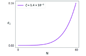
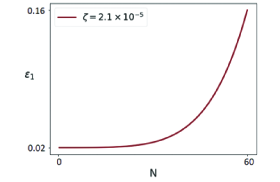
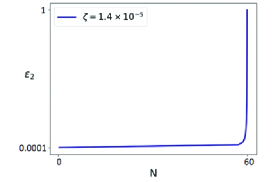
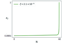
Figure 1: The evolution of the slow-roll parameters $\epsilon_{1}$ and $\epsilon_{2}$ versus the e-folds number during the inflation for the two sample values of $\zeta$.

Another way to seek for inflation and its a graceful exit is the study of the evolution of the Hubble parameter versus the e-folds number. The result is shown in figure 2, which has been plotted for $\zeta=2.1\times 10^{-5}$. As this figure shows, the Hubble parameter during the inflation changes very slowly until inflation ends.

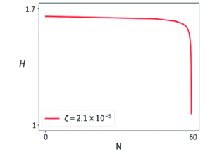
Figure 2: The evolution of the Hubble parameter versus the e-folds number during inflation.

Also, the perturbation parameters are defined in terms of the slow-roll parameters. In this regard, the scalar spectral index and its running are given by  [27, 47, 61, 63, 64]

$$n_{s}\approx 1-2\epsilon_{1}-2\epsilon_{2}\,,$$ (46)

and

$$\alpha_{s}\approx-2\epsilon_{1}\epsilon_{2}-\epsilon_{2}\epsilon_{3}\,.$$ (47)

respectively. The tensor spectral index, in terms of the slow-roll parameters, is defined as

$$n_{T}\approx-2\epsilon_{1}.$$ (48)

Finally, the tenor-to-scalar ratio is given by

$$r\approx 16\epsilon_{1}\,.$$ (49)

By substituting equations (43)-(45) in equations (46)-(49) we obtain the following expressions for the perturbation parameters

$$n_{s}=1-A\sigma-2\,A\,\bigg{(}\frac{\sigma^{2}-\sigma-D}{\sigma}\bigg{)}\,,$$ (50)

$$\alpha_{s}=\Bigg{[}-A^{2}\,\bigg{(}\frac{\sigma^{2}-\sigma-D}{\sigma}\bigg{)}\Bigg{]}\Bigg{[}\sigma+\frac{-\sigma^{3}+\sigma+D}{-\sigma^{2}+\sigma+D}\Bigg{]}\,,$$ (51)

$$n_{T}=-A\,\sigma\,,$$ (52)

and

$$r=8\,A\,\sigma\,.$$ (53)

Finally, by using equation (53) to eliminate the parameter $\sigma$, we get

$$n_{s}=\frac{3}{4}-\frac{r}{8}+2A-\frac{32B}{r}.$$ (54)

$$\alpha_{s}=\left(\frac{r}{8A}-1+\frac{16B}{AR}\right)\left[\frac{-rA}{8}-A^{2}(\frac{-r^{3}+64rA^{2}-1024AB}{-r^{2}+8Ar-128B})\right].$$ (55)

and

$$n_{T}=\frac{-r}{8}.$$ (56)

After obtaining the main perturbations parameters, now we explore the model numerically and compare the results with the observational data. In this regard, we can examine the observational viability of our setup and obtain some constraints on the coupling parameter $\zeta$. Note that, in Ref. [52] it has been shown that only positive values of $\zeta$ lead to the viable cosmology. Therefore, in our analysis, we consider only the positive values of this parameter. Figure 3 shows the behavior of the running of the scalar spectral index versus the scalar spectral index, in the background of the Planck2018 TT, TE, EE+lowE+lensing data [53]. To plot this figure, we have used equations (54) and (55), where the parameters $A$ and $B$ are given by equation (28). This figure and forthcoming figures have been plotted for $0<\zeta\leq 10^{-5}$. We can also study the behavior of the tensor-to-scalar ratio versus the scalar spectral index by using equation (54). The result is shown in figure 4, in the background of the Planck2018 TT, TE, EE+lowE+lensing+BK14+BAO data set [54]. Also, figure 5 shows the tensor-to-scalar ratio versus the tensor spectral index (see equation (56)) in the background of the Planck2018 TT, TE, EE+lowE+lensing+BK14+BAO+LIGO and Virgo2016 data [54]. To plot figures 3-5, we have borrowed the contour plots released by Planck 208 team [53, 54, 55]. This is because, in this paper, we compare the results of the numerical analysis in our model with the Planck observational data. However, the blue regions are the numerical results of our setup which have been obtained from equations (54)-(56). As these figures show, the energy-momentum squared gravity model in some ranges of the model’s parameter space is consistent with observational data. By performing the numerical analysis, we have obtained some ranges of the parameter $\zeta$ which cause the viability of the model in confrontation with different data sets. The constraints are summarized in table 1.

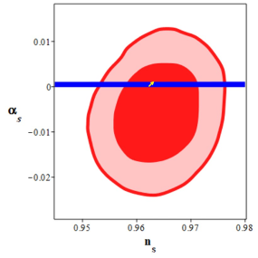
Figure 3: Running of the scalar spectral index versus the scalar spectral index for $0<\zeta\leq 10^{-5}$ (blue region), in the background of Planck2018 TT, TE, EE+lowE+lensing data (red regions). The yellow arrow shows the direction in which the parameter $\zeta$ increases.

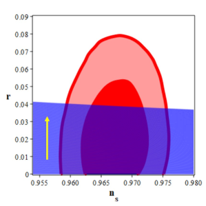
Figure 4: Tensor-to-scalar ratio versus the scalar spectral index for $0<\zeta\leq 10^{-5}$ (blue region), in the background of the Planck2018 TT, TE, EE+lowE+lensing+BK14+BAO data set (red regions). The yellow arrow shows the direction in which the parameter $\zeta$ increases.

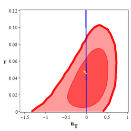
Figure 5: Tensor spectral index versus the tensor spectral index for $0<\zeta\leq 10^{-5}$ (blue region), in the background of the Planck2018 TT, TE, EE+lowE+lensing+BK14+BAO+LIGO and Virgo2016 data (red regions). The yellow arrow shows the direction in which the parameter $\zeta$ increases.

Table 1: The ranges of the parameter $\zeta$ $\left(\frac{s^{4}}{kg^{2}}\right)$ in which the tensor-to-scalar ratio, the scalar spectral index, its running and the tensor spectral index of the $\zeta\,\textbf{T}^{2}$ gravity model are consistent with different data sets.

		Planck2018 TT, TE, EE+lowE	Planck2018 TT, TE, EE+lowE	Planck2018 TT, TE, EE+lowE
		+lensing	+lensing+BK14+BAO	lensing+BK14+BAO
				+LIGO$\&$Virgo2016
	$68\%$ CL	$\zeta\leq 1.6\times 10^{-3}$	$0<\zeta\leq 1.4\times 10^{-5}$	$0<\zeta$
	$95\%$ CL	$0<\zeta\leq 1.6\times 10^{-3}$	$0<\zeta\leq 2.1\times 10^{-5}$	$0<\zeta$

After studying the perturbation’s parameters numerically and obtaining some constraints on the model from the observational data, it seems interesting to seek the abundance of the the fluid $\rho$ with $\omega=\frac{1}{3}$ (corresponding to radiation component). For this purpose, we rewrite equation (18) in terms of the density parameters $\Omega$ as

$$1=\Omega_{{rad}}+\Omega_{{\Lambda}}-{\Omega^{2}_{{rad}}}\Omega_{{\zeta}}\,,$$ (57)

Where

$$\Omega_{{rad}}={\frac{\kappa\,\rho}{3{H}^{2}}}\,,\quad\Omega_{{\Lambda}}={\frac{\Lambda}{3{H}^{2}}}\,,\quad\Omega_{{\zeta}}={\frac{3\lambda\,{H}^{2}}{2{\kappa}^{2}}}\,,$$ (58)

With $rad$ presenting the radiation component. As our numerical analysis has shown, the strength of the energy-momentum squared gravity in our model is small ($0<\zeta\leq 2.1\times 10^{-5}$). This means that even for small strength of the energy-momentum squared gravity, it is possible to get the observationally viable inflationary model. In this sense, to study the abundance of the the fluids in our model, we adopt small value of $\Omega_{\zeta}$ as $\Omega_{\zeta}=0.001$. Then, we find the abundance of $\Omega_{r}$ and $\Omega_{\Lambda}$ at $68\%$ CL and $98\%$ CL, for this adopted value of $\Omega_{\zeta}$. The result is shown in figure 6. According to our analysis at $68\%$ CL, we have $\Omega_{r}=0.908\pm 0.003$ and $\Omega_{\Lambda}=0.091\pm 0.003$.

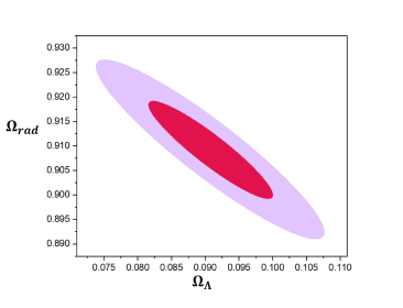
Figure 6: The abundance of $\Omega_{r}$ and $\Omega_{\Lambda}$ at $68\%$ CL (red region) and $98\%$ CL (plum region), for $\Omega_{\zeta}=0.001$.

5 Conclusion

In this paper, we have studied the cosmological dynamics of the energy-momentum squared gravity. In this regard, we have considered an additional term in the Einstein-Hilbert action as $\zeta\,\textbf{T}^{2}$, where $\zeta$ is a positive constant coupling and $\textbf{T}^{2}=T_{\mu\nu}\,T^{\mu\nu}$. We have presented the Einstein’s field equations in $\zeta\,\textbf{T}^{2}$ gravity model and also studied the conservation law via the energy-momentum tensor. We have shown that, by adding a $\zeta\,\textbf{T}^{2}$ term to the action, the energy momentum of the matter fields breaks. However, if we consider an effective energy-momentum tensor, the conservation law would be satisfied. After that, by assuming the FRW metric as the background, we have obtained the Friedmann equations in this setup. In this regard, we have introduced the effective energy density and the effective pressure, by which we have shown the conservation of the effective energy density in the energy-momentum squared gravity model.

Then, we have studied the inflation phase in this model. By obtaining the slow-roll parameters in this model, we have expressed the perturbation parameters in terms of the model’s parameters. By performing a numerical analysis on the scalar spectral index, its running, tensor spectral index and tensor-to-scalar ratio, we have studied the viability of the $\zeta\,\textbf{T}^{2}$ model in the context of the inflation. according to our analysis, Planck2018 TT, TE, EE+lowE+lensing+BK14+BAO+LIGO and Virgo2016 data doesn’t give any constraint on the coupling parameter $\zeta$. However, it is possible to set constraints on $\zeta$ by considering the Planck2018 TT, TE, EE+lowE+lensing and also, Planck2018 TT, TE, EE+lowE+lensing+BK14+BAO data sets.

In summary, the $\zeta\,\textbf{T}^{2}$ gravity model, which lead to the bounce at early universe, is an observationally viable inflation model with $0<\zeta\leq 2.1\times 10^{-5}$.

Appendix

We have the following Lienard differential equation

$$\ddot{H}+AH\dot{H}+BH^{3}=0\,,$$

where

$$A=\frac{4\,\zeta}{\kappa}$$

and

$$B=\frac{-27\,\zeta}{\kappa}+\frac{2\,\Lambda}{\kappa^{2}}\,$$

By assuming $H\equiv y$, we can rewrite the above Lienard equation as follows

$$\ddot{y}+f(y)\dot{y}+g(y)=0\,,$$

where

$$f(y)=A\,y\,,$$

and

$$g(y)=B\,y^{3}\,.$$

Now, we define $w(y)=\dot{y}$ and by which we convert our Lienard equation to the Abel differential equation of the second kind as

$$ww^{\prime}+f(y)w+g(y)=0\,,$$

with $ww^{\prime}=\ddot{y}$ and $w^{\prime}\equiv\frac{dw}{dy}$. By introducing $z=\int F(y)dy$, with $F(y)=-Ay$ and $G(y)=-By^{3}$, the Abel equation takes the following canonical form

$$ww_{,z}=w+\phi(z)\,,$$

where $``,z$” demonstrates derivative with respect to $z$, and

$$\phi(z)=\frac{G(y)}{F(y)}\,.$$

Considering that

$$z=-\frac{Ay^{2}}{2}\,,$$

we find the following expression for $\phi(z)$

$$\phi(z)=\frac{B}{A}\,y^{2}\,,$$

leading to

$$ww_{,z}=w+\frac{B}{A}\,y^{2}=w+D\,z\,.$$

By defining $k(z)=Dz$, we get

$$ww_{,z}=w+k(z)\,,$$

which has the following solution

$$z={\cal{C}}\exp\bigg{(}-\int{\frac{\sigma d\sigma}{\sigma^{2}-\sigma-D}}\bigg{)}\,,\quad w={\cal{C}}\sigma\exp\bigg{(}-\int{\frac{\sigma d\sigma}{\sigma^{2}-\sigma-D}}\bigg{)}\,.$$

Now, we can obtain the Hubble parameter and its derivatives. From $y\equiv H$ and $z=-\frac{Ay^{2}}{2}$, we find

$$H=\left(\frac{-2z}{A}\right)^{\frac{1}{2}}\,.$$

Using $\dot{H}=\dot{y}=w$, we obtain

$$\dot{H}=\sigma\,z\,.$$

Also, from $\ddot{H}=ww^{\prime}$ and considering that $\frac{dw}{dy}\equiv\frac{dw}{dz}\frac{dz}{dy}$, we get

$$\ddot{H}=-A\left(\frac{\sigma+D}{\sigma}\right)H\dot{H}\,.$$

References

- [1] Guth, A., Phys. Rev. D, 23, 347 (1981).
- [2] Linde, A. D, Phys. Lett. B, 108, 389 (1982).
- [3] Albrecht A., & Steinhard, P., Phys. Rev. D, 48, 1220 (1982).
- [4] Linde, A. D. 1990, Particle Physics and Inflationary Cosmology (Harwood Academic Publishers, Chur, Switzerland).
- [5] Liddle, A. & Lyth, D. 2000, Cosmological Inflation and Large-Scale Structure, (Cambridge University Press).
- [6] Lidsey, J. E. et al., Abney, Rev. Mod. Phys., 69, 373 (1997).
- [7] Lyth, D. H. & Liddle, A. R. 2009, The Primordial Density Perturbation (Cambridge University Press).
- [8] Maldacena, J. M., JHEP, 0305, 013 (2003).
- [9] Bartolo, N., Komatsu, E., Matarrese, S. & Riotto, A., Phys. Rept., 402, 103 (2004).
- [10] Chen, X., Adv. Astron., 2010, 638979 (2010).
- [11] De Felice, A. & Tsujikawa, S., Phys. Rev. D, 84, 083504 (2011).
- [12] De Felice, A. & Tsujikawa, S., JCAP, 1104, 029 (2011).
- [13] Nozari, K. & Rashidi, N., Phys. Rev. D, 88, 023519 (2013).
- [14] Nozari, K. & Rashidi, N., Advances in High Energy Physics, https://doi.org/10.1155/2016/1252689 (2016).
- [15] Nozari, K. & Rashidi, N., Physical Review D, 93, 124022 (2016).
- [16] Rashidi, N. & Nozari, K., International Journal of Modern Physics D, 27, 1850076 (2018).
- [17] Nozari, K. & Rashidi, N., The Astrophysical Journal 863, 133 (2018).
- [18] Nozari, K. & Rashidi, N., The Astrophysical Journal, 882, 78 (2019).
- [19] Rashidi, N. & Nozari, K., The Astrophysical Journal, 890, 58 (2020).
- [20] Nojiri, S. & Odintsov, S. D, Phys. Rept. 505, 59-144 (2011).
- [21] Nojiri, S., Odintsov, S.D. $ Oikonomou, V.K., Phys.Rept., 692, 1-104 (2017).
- [22] Sotiriou, T. P., & Faraoni, V., Rev. Mod. Phys 82, 451 (2010).
- [23] Nojiri, S., & Odintsov, S. D., Phys. Rept 505, 59 (2011).
- [24] Starobinsky, A. A., JETP Lett 86, 157 (2007).
- [25] Nojiri, S., & Odintsov, S. D., & Oikonomou, V. K., Phys. Rev. D 93, 084050 (2016).
- [26] Nojiri, S., & Odintsov, S. D., & Oikonomou, V. K., Mod. Phys. Lett. A 31, 1650172 (2016).
- [27] Nojiri, S., & Odintsov, S. D., & Oikonomou, V. K., JCAP, 1605, 046 (2016).
- [28] Felice, A. De., & Tsujikawa, S., Living Rev. Rel 13, (2010).
- [29] Nojiri, S., & Odintsov, S. D., & Oikonomou, V. K., Phys. Rept 692, 1 (2017).
- [30] Song, Y. S., & Hu, W., & Sawicki, I., Phys. Rev. D 75, 044004 (2007).
- [31] Nojiri, S., & Odintsov, S. D., & Oikonomou, V. K., Class. Quantum. Grav 33, 125017 (2016).
- [32] Nojiri, S., Odintsov, S.D., & Oikonomou, V.K., DOI: 10.1016/j.nuclphysb.2019.02.008 (2019).
- [33] Odintsov, S.D., & Oikonomou, V.K., Phys. Rev. D 99, 064049 (2019).
- [34] Budhi, R. H. S., DOI: https://doi.org/10.1088/1742-6596/1127/1/012018 (2017).
- [35] Bertolami, O., Boehmer, C. G., Harko, T., & Lobo, F. S. N., Phys. Rev. D 75, 104016 (2007).
- [36] Harko, T., Phys. Lett. B 669, 376 (2008).
- [37] Thakur, S., Sen, A. A., & Seshadri, T. R., Phys. Lett. B 696, 309 (2011).
- [38] Bertolamim O., & Paramos, J., Class. Quantum Grav. 25, 5017 (2008).
- [39] Boehmer, C. G., Harko, T., & Lobo, F. S. N., Astropart. Phys. 29, 386 (2008).
- [40] Faraoni, V., Phys. Rev. D 80, 124040 (2009).
- [41] Harko,T., & Lobo, F. S. N., The European Physical Journal C-Particles and Fields 70, 373 (2010).
- [42] Nojiri, S., & Odintsov, S. D., Phys. Lett. B 599, 137 (2004).
- [43] Allemandi, G., Borowiec, A., Francaviglia, M., & Odintsov, S. D., Phys. Rev. D 72, 063505 (2005).
- [44] Bertolami, O., & Paramos, J., Phys. Rev. D 77, 084018 (2008).
- [45] Faraoni, V., Phys. Rev. D 76, 127501 (2007).
- [46] Harko, T., Phys. Rev. D 81, 044021 (2010).
- [47] Rajabi, F., & K. Nozari, Phys. Rev. D 96, 084061 (2017).
- [48] Harko, T., Lobo, F. S.N., Nojiri, S., & Odintsov, S D., Phys. Rev. D 84, 024020 (2011).
- [49] Sahu, S. K., Tripathy, S. K., Sahoo, P. K., & Nath, A., Chinese Journal of Physics, 55, 862-869 (2017).
- [50] Wu, J., Li, G., Harko, T., & Liang, S.-D., The European Physical Journal C 78, 430 (2018).
- [51] Pawar, D .D., & Shahare, S. P., https://doi.org/10.1016/j.newast.2019.101318 (2019).
- [52] Roshan, M., & Shojai, F., Phys. Rev. D, 94, 044002 (2016).
- [53] Planck Collaboration: Aghanim, N., et. al. (2018) [arXiv:1807.06209[astro-ph.CO]].
- [54] Planck Collaboration: Akrami, Y., et. al. (2018) [arXiv:1807.06209[astro-ph.CO]].
- [55] Planck Collaboration: Akrami, Y., et. al. (2018) [arXiv:1807.06211[astro-ph.CO]].
- [56] Board, C. V. R. & J. D. Barrow, Phys. Rev. D 96, no.12, 123517 (2017).
- [57] Nari, N., & Roshan, M., Phys. Rev. D 98, 024031 (2018).
- [58] Sotiriou, T. P., & Faraoni, V., Class. Quant. Grav. 25, 205002 (2008).
- [59] Bertolami, O., & Lobo, F. S. N., & Paramos, J., Phys. Rev. D 78, 064036 (2008).
- [60] Polyanin, A. D. & Zaitsev, V. F., 2003, Handbook of Exact Solutions for Ordinary Differential Equations, (2nd Edition , Chapman & Hall/CRC, Boca Raton).
- [61] Martin, J., Ringeval, C., & Vennin, V., Phys. Dark Univ. 5-6, 75 (2014).
- [62] Leach, S. M., Liddle, A. R., Martin, J., & Schwarz, D. J., Phys. Rev. D 66, 023515 (2002).
- [63] Bamba, K., Nojiri, S., Odintsov, S. D., & Saez-Gomez, D., Phys. Rev. D 90, 124061 (2014).
- [64] Bhattacharjee, S., Santos, J.R.L., Moraes, P.H.R.S., & Sahoo, P.K., Eur. Phys. J. Plus 135, 576 (2020).