BROUTE: a benchmark suite for the implementation of standard vehicle routing algorithms

Abstract

We introduce BROUTE, a benchmark suite for vehicle routing optimization algorithms. We define a selection of algorithms traditionally used in vehicle routing optimization. They capture essential features that are also relevant in optimization algorithms for different application domains, like local search move evaluation, memory allocation, dynamic programming, or insertion and deletion from a list. Each algorithm is deterministic. We implement these benchmark algorithms using a selection of programming languages and different data structures. BROUTE is free, open-source, and can be used to inform early decisions in projects that involve programming, such as which language to use.

1 Introduction

When it comes to implementing optimization algorithms and routing algorithms, some important design decisions such as the choice of the programming language must be made early. While most programming languages are Turing-complete, thus allowing to run any deterministic algorithm, they vary in many aspects including conciseness, ease of writing, ease of reading, ease of debugging and runtime performance. Many of these aspects are subjective in nature, but runtime performance can be measured objectively. We introduce a benchmark suite for vehicle routing optimization algorithms called BROUTE, available at https://github.com/fa-bien/broute, which focuses on CPU effort. CPU effort is especially relevant when running the final version of a program, as it is a direct measure of performance. However it also matters while developing and debugging, as these tasks typically involve repeatedly running the program and waiting for the runs to complete.

The goal of this suite is to inform early design decisions when programming optimization algorithms, such as the choice of the programming language, or how to represent a distance matrix. Readers may already know a few programming languages and know both (i) which one they appreciate using the most and (ii) which one offers the best performance, but they do not necessarily have a quantified assessment of the trade-off between performance and convenience, i.e. of the performance cost of convenience. Other readers may need to decide which programming language their new student should learn and use for the implementation of their research work. Others may elect to program using Julia because it makes them more productive, but still want to know what kind of performance to expect when compared to C++. Some will want to find out, given the hardware and software they have access to, which language is the most efficient for which task. These decisions can all be informed by using BROUTE.

1.1 Scope of this study

We provide the means to compare the reasonably efficient implementation of various algorithms used in combinatorial optimization, within a given experimental setting. In particular, we look at five algorithms that are commonly used in vehicle routing optimization. However these algorithms capture features that are also common in other domains of optimization, such as modifying subsequences, inserting and removing elements in a sequence, or other operations on graphs. The five algorithms are implemented using different programming languages. We put ourselves in the situation of a programmer with limited experience, for example a student, having to implement these algorithms. For the time being all benchmarks are implemented in C++, Python, Java, JavaScript, Rust and Julia. We also assess the impact on performance of some implementation decisions, e.g. using a flat matrix representation.

Our goal is not to provide the most efficient implementation of each algorithm for a set of languages, or even to use the most efficient algorithm to solve the given problems. In fact, the value of the run time performance comparisons is independent from the efficiency of the algorithms, as long as all implementations are of the same algorithms and use comparable data structures. Nonetheless, we believe the algorithms used (i) capture an interesting range of features encountered in many routing algorithms and (ii) are reasonably good implementations of reasonably efficient algorithms. Additionally, we welcome the addition of new benchmark algorithms to BROUTE in the future, which might then allow a comparison of the efficiency of different algorithms. However, this falls outside the scope of this contribution.

Drawing general conclusions about which programming language is the best, or yields the most productivity, or even runs the fastest, is of limited interest: software evolves fast, hardware architectures evolve as well and compilers have to adapt. Some outcomes observed in the example experimental study in Section 5 may have been different a few years ago, and might be different on a different platform. However, even though benchmark results depend on constant software and hardware evolution, the tools to provide these results are independent from it and can be used in any experimental setting, now or in the future. BROUTE is such a tool.

Readers looking for state-of-the-art implementations of algorithms for vehicle routing, including efficient data structures, may find these contributions interesting: LKH (Helsgaun,, 2000, 2009; Taillard and Helsgaun,, 2019) is likely the most efficient implementation of local search for the TSP currently in existence, and tackles instances with several million nodes efficiently; a linear time Split algorithm, which is employed in some of the best known metaheuristics for VRPs, is provided by Vidal, (2016); a generic state-of-the-art branch-and-price code is provided by Sadykov and Vanderbeck, (2021).

1.2 What is measured

In all proposed benchmarks, the CPU time of the benchmarked algorithm is measured. Every other task, such as reading input data or constructing an initial solution for local search benchmarks, is not measured. If an auxilliary graph needs to be constructed every time the algorithm is run, then we also measure the construction of said auxilliary graph. This is the case for benchmarks maxflow and espprc. We do not, however, measure the time required to allocate this auxiliary graph in memory: this typically happens once when a program starts, then the same memory can be used many times.

In general, compilation time is not measured. However, some implementations do just-in-time (JIT) compilation, for example Julia, JavaScript, Pypy, Numba and Java. In such cases, this JIT compilation time is included in the running time of the algorithm. In general we measure clock time, i.e. the CPU budget used by the algorithm. In the case of JavaScript we measure wall time as we are not aware of any way to measure clock time in JavaScript.

In order to represent a tour in various heuristics, we use variable-size vectors. Dynamic size containers are intuitive to use in algorithms for vehicle routing, for instance to insert or delete a vertex from a tour. Such containers can also be used to represent solutions in other domains, e.g. scheduling or any application that requires the representation of sequences of variable length. Inserting and deleting elements in a vector has linear worst-case time complexity. However, for heuristics it can still be a good idea to use vectors rather than, say, linked lists, since neighborhood exploration typically requires to evaluate many moves then perform only one of these moves. The complexity of performing a move is thus a secondary concern and unlikely to be a performance bottleneck. Additionally, performing certain moves can actually be more efficient using a vector than using a linked list, e.g. inverting a subsequence in the context of 2-opt. There exist a variety of data structures for vehicle routing, for example one can use arrays of successors (Cacchiani et al.,, 2014); their size is dynamic but they do not require further memory allocation and allow insertion and deletion in $\mathcal{O}(1)$. Efficient data structures for TSPs are discussed by Helsgaun, (2000). One conclusion is that below 1000 cities, some sophisticated data structures are outperformed by arrays and lists, due to their time overhead. Additionally, their implementation is not simple.

1.3 Limitations

Benchmarks are by definition limited in scope. Any given benchmark measurement is only valid within a certain environment. In our case such environmental factors include the choice of compilers, compiler versions, operating system and CPU family. Therefore all results are to be taken as indicators but not absolute truths. The intent of this study is not to declare a language the winner because it is consistently faster than others by a few percents, but rather to assess what kind of performance losses can be expected by, for example, using Python instead of C++ on a given computing cluster. Another example is to assess what kind of performance gains can be achieved by using a JIT compiler for Python. One could also determine differences in performance between different C++ compilers.

Additionally, there are some implicit conditions for the good functioning of interpreters and compilers. For instance Pypy is advertised to work better when things are “kept simple”, which is generally good advice regardless of the compiler. However, this typically requires discipline.

2 The benchmarks

We consider five different benchmark algorithms that perform tasks commonly encountered in transport optimization. Together they capture key aspects of computationally intensive tasks in heuristics and exact methods for transport optimization, although they do not necessarily use the most efficient algorithm to solve the problem they are tackling. Additionally, we believe that they also capture such aspects for other fields of application of operations research, such as e.g. scheduling. For the sake of simplicity, we consider the symmetric travelling salesperson problem (TSP) as a base problem, i.e. input data are in the form of a symmetric distance matrix while a solution is a permutation. However some benchmark algorithms solve different problems than the TSP based on these TSP data, as described below. Abstract algorithms are providex in Appendix B. The implementations are all available at https://github.com/fa-bien/broute.

All five benchmarking algorithms described below are deterministic. In cases where we want to capture the features of a stochastic algorithm, we simulate randomness in a deterministic fashion for the sake of reproducibility. Additionally, the input provided to them is also deterministic, i.e. each implementation receives the exact same inputs and performs the same operations from these inputs. For that purpose, we generate various instance files, each with a given size $n$, which represents the number of vertices in the graph, and a number $p$ of permutations. A permutation is a solution to the TSP. Vertex coordinates are generated randomly in $[0,100)$. Let $d_{ij}$ be the Euclidean distance between $i$ and $j$, then the distance considered is $c_{ij}=\lfloor 100d_{ij}\rfloor$. Since it is an integer number, it is sufficient to use integer number representation to compute the cost of a TSP solution; however certain benchmarks use floating-point number representation, as explained below. Each instance file contains one $n\times n$ distance matrix as well as $p$ randomly generated permutations, which are used as starting seeds for the algorithms (e.g. as starting solution for 2-opt).

Since the same instance files are given to each implementation, all implementations perform the same operations and return the same result. In order to control result integrity we use a mechanism similar to checksum. The checksum calculation for applying a certain algorithm using a given permutation as starting seed differs based on the algorithm and is explained separately for each algorithm below. The checksum calculation for an instance file is the sum of checksum values over all permutations in that instance file.

Performances are measured per instance file, i.e. each time reported is for running an algorithm $p$ times, using one distance matrix with the $p$ different seed permutations.

2.1 2-opt

The 2-opt heuristic was first described by Croes, (1958). One of the most commonly used heuristics in vehicle routing, 2-opt improves a tour by performing 2-exchanges. A 2-exchange consists in removing two edges from a tour and reconnecting the tour with two other edges. It is equivalent to inverting a sub-sequence of the tour, and can be performed in place using an array or vector solution representation. If the distances are symmetric, then each move can be evaluated in constant time.

The checksum for a given permutation seed is the number of improvements found while applying first-improvement 2-opt until no improving move exists, using this permutation as starting solution.

2.2 Or-opt

Or-opt is a heuristic that was first introduced by Or, (1976). It relies on the exploration of a neighborhood that is a subset of all 3-exchanges. A 3-exchange consists in removing 3 edges from a tour and reconnecting the tour in a different way. Of all these moves, Or-opt only considers those that shift a sequence of 1, 2 or 3 vertices to a different position in the tour. Each move can be evaluated in constant time.

The checksum for a given permutation seed is the number of improvements found while applying first-improvement Or-opt until no improving move exists, using this permutation as starting solution.

2.3 lns: Large neighbourhood search

Large neighborhood search (LNS) was originally introduced in conjunction with constraint programming to solve the vehicle routing problem with time windows (VRPTW) (Shaw,, 1998). Since it has been a very popular method for tackling a wide variety of vehicle routing problems, see e.g. Pisinger and Ropke, (2010).

LNS iteratively (i) copies the incumbent solution, (ii) destroys the copy by removing some vertices from it, (iii) repairs the partial solution by re-inserting previously removed customers in it and (iv) determines whether this newly produced solution becomes the new incumbent solution or not. The method relies, among other things, on randomness. This is an issue since we want each benchmark to be deterministic. To remedy this issue, we design deterministic schemes for both destroying and repairing stages. For each starting seed, we apply a certain number of LNS iterations. At each iteration, the vertices at even indices in the tour are removed. These removed vertices are stored in a vector in the order in which they were removed, i.e. from smallest to largest index. Then the cost of each possible insertion is calculated and the cheapest insertion is performed. Because removed vertices are stored in a vector, the algorithm’s behaviour in case of same-cost insertions is deterministic.

The checksum for a given permutation seed is the total cost of insertions performed while applying 10 iterations of LNS using that permutation as starting solution.

2.4 espprc and espprc-index: Dynamic programming for column generation

Many state-of-the-art exact methods for vehicle routing problems (VRPs) rely on column generation (see e.g. Baldacci et al., (2012)). In such methods, a significant amount of CPU effort is spent solving the pricing subproblem, which differs depending on the problem at hand but is nonetheless often an elementary shortest path problem with resource constraints (ESPPRC). While it can be solved heuristically, in order to establish optimality it eventually needs to be solved exactly as well. For this benchmark we implement a dynamic programming algorithm similar to the one by Feillet et al., (2004) to solve the ESPPRC, albeit without time windows. One difficulty in this problem stems from the existence of negative-cost cycles in the graph.

In order to simulate an environment similar to the one encountered in column generation for VRPs, we derive an ESPPRC instance from each TSP seed permutation by using an auxilliary distance matrix $c^{\prime}$ from the distance matrix $c$, as follows:

1. For each vertex $j$, let $\pi_{j}$ be the cost of arc $(i,j)$, where $i$ is the predecessor of $j$ in the seed permutation.

2. For each arc $(i,j)$, set $c^{\prime}_{ij}$ to $c_{ij}-d_{j}$.

Additionally, we generate resource consumption as follows: we consider 6 resources numbered from 0 to 5, and any vertex $i$ consumes resource $r$ iff the $r^{th}$ bit of $i$’s binary representation is 1 (considering that the first bit is bit 0). That is, in C syntax, iff i & (1 << r) > 0. Capacity is set to 1 for each resource. The algorithm then computes the elementary shortest path with resource constraints on $c^{\prime}$ from 0 to 0 (1 to 1 in Julia).

For this benchmark, floating-point numbers are used to represent cost, even though the values are integer. This is to emulate the usual setting when solving such problems in the context of column generation.

Each label needs (i) a reference to its predecessor, so that paths can be reconstructed and (ii) a collection of references to its successors, in order to recursively propagate dominance and later ignore labels that are successors of an already proved-to-be-dominated label. Rust does not allow that, at least not in the intuitive way where a label is encapsulated in a struct, including references to predecessor and successors. This is because Rust is focused on security, while this type of construct can lead to unsafe operations if not used properly. This means that this benchmark cannot be safely implemented with Rust, even though it is consistent and reliable in all other implementations. In order to remediate this issue, we produce a second implementation of the same algorithm, although in a less intuitive way: all labels are stored in a collection, and the indices in this collection are used in other collections to store all predecessors and successors. This second implementation represents a different benchmark, which we call espprc-index, whereas the base benchmark is called espprc. The version with indices is more tedious to implement, but it may also be more efficient, so we also implement it in languages other than Rust.

The checksum for a given permutation seed is the cost of the shortest elementary path obtained when using that permutation seed to generate the ESPPRC instance, truncated to its integer part.

2.5 maxflow: Maximum flow problem

Another popular framework for the exact solution of routing problems is branch and cut. Branch and cut is typically applied to solve mixed-integer linear programs; it is akin to branch and bound but only considers a subset of all constraints explicitly. Other constraints are generated dynamically when they are found to be violated while exploring the search tree. These constraints are said to be separated. One early success story of branch and cut is actually in application to the symmetric TSP (Padberg and Rinaldi,, 1987), by separating subtour elimination constraints. The separation procedure involves finding a minimum capacity cut, which itself involves solving a maximum flow problem. For this reason the maximum flow problem is important in vehicle routing, and we dedicate one benchmark to solving it. The maxflow benchmark implements the Edmonds-Karp algorithm (Edmonds and Karp,, 1972), which is a specific version of the Ford-Fulkerson (Ford and Fulkerson,, 1956) augmenting path method. The specificity resides in how the augmenting paths are generated.

We derive a capacity graph $C$ from the distance matrix $c$ and a given TSP solution as follows:

1. For each vertex $j$, let $t_{j}$ be the cost of arc $(i,j)$, where $i$ is the predecessor of $j$ in the TSP solution.

2. For each arc $(i,j)$, set $C_{ij}$ to $\frac{c_{ij}}{1000}$ if $c_{ij}>t_{j}$, otherwise set it to 0.

For any starting seed, the capacity graph is generated then the Edmonds-Karp algorithm is applied with 0 as source and every other node as sink. The checksum for that permutation seed is the sum of all maximum flow values thus obtained, truncated to its integer part.

3 Languages and implementations considered

We consider six different programming languages: C++, Python, Java, Julia, Rust and Javascript. Any rule of selection is arbitrary in nature; however we indicate below, for each of these languages, our perceived advantages of these languages, which justify their selection. It is possible to add other languages to this list in the future, and keep the benchmark collection alive in an online form. For a given language several implementations are possible, e.g. one with nested distance matrices and one with flat distance matrices. As a convention, implementations are named in lower-case letters, for example python-flat-matrix. We also use the simplest names for the best implementations, i.e. python uses a nested distance matrix because it performs better than python-flat-matrix, but pypy uses a flat matrix because it performs better than pypy-nested-matrix. Language versions and options are summarised in Appendix A.

For each language, we may consider multiple implementations, which differ by which mechanisms or library they use. For instance with Python we can compare an implementation using native lists against an implementation using Numpy arrays. Implementations are detailed individually below for each language. The code for all implementations can be found at https://github.com/fa-bien/broute.

It is difficult to properly measure the popularity of a programming language. There exist rankings, for example based on online searches (TIOBE,, 2020) or on GitHub contributions (GitHub,, 2020). All these approaches have flaws. Basing an index on online searches is subject to all the biases and exploits that target online search. Measuring GitHub contributions is not clear, as there is no trivial way to decide what should count among repositories, number of lines written, number of commits, etc. Ultimately, language popularity for its own sake does not need to be a crucial factor in the choice of a programming language, especially for academic research. These aspects seem more important to us:

• The programs written in a given programming language should be easily run on any computer. For that reason, we only look at languages that are free and work under multiple operating systems. The ability to run under Linux is especially important, since it is typically the operating system of high-performance computing (HPC) clusters (TOP500,, 2021).

• The language should be well documented, but also have online resources for support. This in fact also depends on popularity.

3.1 C++

C++ is one of the most popular programming languages in the World, and has been so for decades. Among its many features there is good runtime performance. In fact the performance is good enough that whole operating systems can be written in C++, for example Microsoft Windows. C++ has many features and it is often possible to implement the same algorithm using different subsets of the language; one criticism is that people and teams evolve into using only their own subset of the language.

We develop two C++ implementations of every benchmark, using the C++98 and C++14 standards, which we call c++98 and c++14. they both use a flat distance matrix. With C++98 we use references to objects, while with C++14 we use smart pointers such as shared_ptr. Comparing these two implementations will allow us to evaluate the cost of smart pointers.

For each benchmark the reference CPU time is provided by the c++98 implementation. We also develop a variant of c++14 using a nested distance matrix, and another using static arrays.

3.2 Python

Python is another of the most popular programming languages in the World, especially for tasks of machine learning in recent years. The base Python implementation is called python and uses a nested distance matrix. There is also an implementation using a flat distance matrix, called python-flat-matrix, and one using a nested distance matrix wrapped in function calls, called python-nested-matrix-function.

One issue with Python is that much of the code is not compiled, rather directly interpreted, which can lead to poor performance. One way to address that issue is to rely on libraries that are implemented in C, however that is not always possible. We consider alternative implementations in Python, all bringing different solutions to this issue.

The simplest way to speed up the run time of a Python program is to run this program with Pypy (Pypy,, 2021) instead of the standard CPython interpreter. Pypy uses JIT compilation to speed things up. There is no need to modify the Python program, which is a strong advantage compared to library-based solutions or annotation-based solutions. Pypy’s website claims that it is on average 4.2 times faster than CPython (Pypy,, 2021), however this is just an average and actual numbers may vary a lot depending on the benchmark. We use both the python and python-flat-matrix implementations with Pypy, resulting in pypy-nested-matrix and pypy implementations, respectively.

We also implement the benchmarks using Numpy arrays instead of standard Python lists. Numpy is one of the most popular external libraries for Python; it is coded in C for runtime performance (Harris et al.,, 2020). Numpy performs especially well when using array operations, for instance matrix multiplication. However the benchmarks that we consider do not take advantage of Numpy functions, only of its array data structure. Since Numpy provides multi-dimensional arrays, we use a two-dimensional array to represent the distancematrix. Additionally, we consider a flat matrix in implementation numpy-flat-matrix.

Numpy itself does not provide any kind of JIT compilation, but another Python package, Numba, performs JIT compilation when using Numpy arrays. Numba requires code annotation, therefore we annotate the Numpy implementations to take advantage of them with Numba.

3.3 Java

Java is a very popular programming language of the past two decades. Java code is compiled to bytecode, which is then run by a virtual machine (VM). The bytecode compiled on one computer can be run by a VM on another computer. Nonetheless, JIT compilation to native code happens dynamically at run time. The syntax is based on C/C++ syntax. The base Java implementation, java, uses a flat distance matrix and a ArrayList<Integer> object to represent a tour. We also implement a version with nested distance matrix, java-nested-matrix, as well as a version with static arrays to represent a tour, java-static-arrays.

3.4 Julia

Julia is a relatively recent programming language. It is a general-purpose language but it is also particularly aimed at computationally intensive tasks such as numerical analysis (Bezanson et al.,, 2017). Version 1.0 was released in 2018 and the language is well-documented and has a strong community.

Compilation happens in a JIT fashion. Like Numpy but unlike all other programming languages considered, Julia supports multi-dimensional arrays, therefore a native two-dimensional array can be used to represent a distance matrix. We also develop an implementation using flat matrix representation in Julia, called julia-flat-matrix; we will determine which version is better through experiment.

One valuable feature of Julia is the fact that projects have an environment, including package dependencies with specific versions. The language makes it easy to instantiate the project environment, i.e. recreate the same environment in which the project was developed, with the same packages in the same versions. This provides safety from backward-compatibility-breaking library updates.

One notable issue with Julia is the inability to generate a compiled binary executable file. In general, in order to run a Julia program, one must install the Julia ecosystem. There are active projects to remedy this, but we are not aware of any easy one-command solution.

3.5 Rust

Rust is also relatively recent, with version 1.0 released in 2015. It is a general-purpose language with an emphasis on memory safety and on performance. Notable software using Rust include Firefox, Dropbox and Cloudflare (The Rust Team,, 2021).

Programs in Rust are pre-compiled, like in C++ for instance. Like Julia, the language is well documented and has a strong community. Also like Julia, projects have an environment, and it is easy to recreate the environment for a given project, including dependencies and their specific version, which again provides safety from backward-compatibility-breaking library updates. The rust implementation uses a flat matrix representation.

3.6 JavaScript

JavaScript is likely one of the most popular programming languages in the World, as it is used on countless websites as well as mobile applications based on web technology. JavaScript is not expected to perform as well as, say, C++. However there are several reasons why it can be appealing to implement routing algorithms in JavaScript:

• Any program written in JavaScript can run on virtually any computer with a modern web browser, including smartphones.

• Integrating JavaScript with a web interface is especially easy.

• JavaScript engines have received considerable attention from major companies and been the subject of fierce competition in relation with web browsers engines. As a result they have seen vast performance improvements over the years and the trend is likely to continue.

We use Node.js, which allows to run JavaScript programs from the command line. This means that there is in fact not even the need for a web browser. Node.js currently uses Google Chrome v8’s JavaScript engine (nodejs.org,, 2021).

The javascript implementation uses a flat matrix representation but there is also an implementation using nested matrix representation, called javascript-nested-matrix.

3.7 Considerations on how to implement a distance matrix

Perhaps the most straightforward way to implement a distance matrix in a number of languages is to use nested arrays, i.e. each element of the main array is an array representing a row of the distance matrix. This is typically done in C++, Java, Python (although the structure is officially called a list and not an array), Javascript. C and C++ use pointers to achieve that effect. All these languages use the same C syntax for looking up values in the distance matrix: the distance between vertices $i$ and $j$ using distance matrix $d$ is written d[i][j].

Another easy way to implement a distance matrix is to use what we call from here on a flat distance matrix representation, which is a single-dimensional array containing all distance values. Assuming indices start at 0, the distance from $i$ to $j$ in array $d$ can be coded as d[i*n+j], where $n$ is the total number of vertices. This representation guarantees that the whole distance matrix is stored in contiguous memory. Additionally, looking up in arrays also takes time, so one lookup is better than two. The drawback is that we have to pay a multiplication and an addition for each lookup, and that lookups have to be wrapped in a function call for the sake of readability. Such function calls can usually be inlined, i.e. the function content is substituted to the function call, so there should be no runtime penalty from using a function call. In general we expect a speedup from using a flat representation. We implemented some of the benchmarks with both flat and nested matrix representation in order to determine if there are significant performance differences.

There are a few cases where the above considerations on using a flat representation do not apply: Python does not allow inlining, while Numpy and Julia provide multi-dimensional arrays. Nonetheless we also wrote a flat matrix version of these implementations, in order to elicit any difference in performance.

3.8 Other general cross-language considerations

Here we discuss considerations that are subjective in nature, as they relate to individual experience implementing all benchmarks in all languages. The author’s experience with all considered programming languages is heterogeneous, which can cause bias in the perception of the ease of implementation in a given language. To add to the subjectivity, each benchmark is first implemented in Python then in other languages, with Rust typically being the last one to be implemented. Therefore the languages implemented last represent supposedly easier tasks, due to increased familiarity with the algorithm. For all reasons mentioned above, measuring the time spent implementing each benchmark in each language would be meaningless, therefore we limit ourselves to subjective opinion here. Keeping this in mind, we see a subset of perceived easy languages, as in “easy to program in and get things running with the expected outcome”, which consists of Python, Julia and JavaScript. These easy languages typically allow to program the same algorithms faster than the other ones with the same results, performance considerations aside. On the other hand, we found the process of getting benchmarks to work with Rust to be much more tedious than with any other language, although this is certainly due to lack of experience. Nonetheless, the JavaScript implementation was typically easier than the C++ or Java ones despite having more experience with C++ and Java, so experience does not explain everything. Ultimately, there is little doubt that any experienced programmer in any of these languages would have no trouble implementing any of these benchmarks. Nonetheless, this programmer with experience in mostly C++ and Python implemented every benchmark faster in Python, JavaScript or Julia than in C++.

We also want to underline that no matter the language, it is possible to write both efficient and inefficient code. Familiarity and experience are beneficial; beginners in a language are more likely to write inefficient code. This being said, not every language is equal when it comes to documenting how to write efficient code. We note that the official Julia documentation has a whole section dedicated to that topic (Julia Documentation,, 2021). There also exists an automated tool to detect inefficient code patterns, based on the official documentation (JunoLab,, 2020).

4 Implementation-specific notes

4.1 Python

CPython, Python’s official interpreter, does not allow to inline functions. Since using a flat matrix requires to wrap matrix value lookup in a function, using a flat distance matrix in Python is not beneficial. It would of course be possible to inline by hand, i.e. formulate the correct 1-dimensional index in the matrix for every lookup, but that would be impractical and defeat the purposes and philosophy stated in Section 1. Running Python code that uses a flat representation with a JIT compiler (e.g. Pypy, Numba) introduces automatic inlining and is likely to remedy this.

On the ESPPRC benchmark, a label needs to store information about which customers have already been visited in the partial path it represents. In Python, preliminary testing reveals that using a set of integers for that purpose is twice as fast as using a vector of booleans. Similar preliminary testing in C++ reveals the opposite: using an array of booleans is faster. This is the behaviour we would expect in general, the observation on Python is the surprising one here. There are two reasons for this expectation: (i) copying an array, represented in contiguous memory, can in general be performed faster than copying a set structure and (ii) lookup in an array is performed in $\mathcal{O}(1)$ while lookup in a set is performed in $\mathcal{O}(log(n))$.

4.2 Julia

Julia has native multi-dimensional arrays, which may be more efficient than a flat representation. We will determine which version to use based on experiment. Since Julia’s arrays start with index 1, the code for flat representation lookup of the distance between vertices $i$ and $j$ in matrix $d$ is d[i*n-n+j]. It is worth noting that it involves one subtraction on top of the addition and multiplication used for 0-indexed languages.

4.3 JavaScript

All benchmarks are repetitive in nature, as they successively perform similar operations with different input data. In JavaScript, when our implementation loads 40 instances and performs the same benchmarking operations on all 40 them, we observe a significant performance hit after a few instances (2-5 times slower). In order to remedy this, we re-start the program individually for each instance. Advanced knowledge of this specific JavaScript engine might allow to remove that performance hit, but this is clearly outside the scope of this study. However it is worth noting that this can be a concern in general.

4.4 Numba

Numba is not yet feature-complete for Numpy. A direct consequence is that some benchmarks cannot be implemented for Numba. For example numpy.insert() is not implemented, but this function is needed for the $lns$ benchmark, therefore the $lns$ benchmark cannot be implemented with Numba. Additionally, we were not able to implement the ESPPRC benchmark in a satisfying manner. In our experience, Numba error messages are sometimes unrelated to the issue causing them, or too obscure to make sense, keeping in mind the premises of this paper. It would likely be possible to implement a dynamic programming algorithm for the espprc benchmark using Numba’s JIT compilation features, however our conclusion is that it would not be possible to do so without advanced knowledge of Numba.

Still, Numba is relevant enough to be benchmarked and its current performance is an indication of what to expect in years to come, as the project matures.

4.5 Java

The ecosystem of Java implementations and versions can be hard to navigate. There exist multiple compilers, multiple virtual machines, and there is a new Java version every 6 months, sometimes breaking backwards compatibility. The official reference implementation is OpenJDK since version 7 (Oracle Corporation,, 2011). We use OpenJDK version 11, which is the current long-term support version as of writing this article.

4.6 Rust

As mentioned in Section 2.4, Rust does not allow a given struct to have multiple references to the same struct type. For this reason, a different implementation of the espprc benchmark is needed. In general Rust puts restrictions on what constitutes valid code, for the sake of safety. This is a valuable feature in systems programming, which is the main application that Rust was designed for. This also means that writing code that compiles and runs is actually a more tedious task, but that once the code compiles, there is also a higher chance that it will run according to expectations, like with the Ada programming language for instance.

In the context of this study, these benefits did not appear relevant however: each benchmark was programmed in all other languages as well, providing the same results as with the Rust implementation, while no evidence of memory leak was observed. As mentioned above, The Rust implementation was typically way more time-consuming than other implementations, although one reason for that is lack of experience. Nonetheless, in the context of this study, the generally assumed benefits of using Rust are not apparent, with the notable exception of good runtime performance.

5 Experiments

In this section, we provide examples of some possibilities offered by BROUTE and perform topic-specific comparisons for a given hardware and software setup. The computer is a cluster where each node has an Intel Xeon E5-2650 v3 CPU, 20 cores per CPU, 3 GHz, running Linux. The cluster is shared and it is not possible to reserve an entire node. The compiler and interpreter versions used are described in Appendix A. For every benchmark and every instance, CPU times are reported as a ratio of a reference time for that benchmark and instance. In practice, for each benchmark and instance, the reference time is the time required by the c++14 implementation for that benchmark and that instance. Therefore the c++14 implementation always has a CPU ratio of 1.

5.1 Benchmark data

Each instance file contains one $n\times n$ distance matrix as well as $p$ randomly generated permutations, which are used as starting seeds for the algorithms (e.g. as starting solution for 2-opt). For $n$ taking each value of $\{20,40,60\}$ and fixing $p=1000$ we generate 40 instance files, for a total of 120 instance files. Each instance file contains 1000 permutations, therefore involves running each benchmark 1000 times. As mentioned in Section 2, distances are Euclidean distances multiplied by 100 and truncated to their integer part. In the following, each data point represents the total CPU time for running one benchmark implementation for each of the 1000 permutations of one given instance file.

These data points are represented in two types of charts: box plots and performance profiles. Box plots contain different boxes for different values of $n$, and these boxes are always displayed, from left to right, in the order in which they appear in the legend from top to bottom. Performance profiles aggregate all data points for a given implementation into one profile, i.e. one curve. A performance profile is a chart that indicates, for a given level of performance, the ratio of data points produced with that performance level or a better one. In our case, the performance level is the CPU effort required to produce a data point, as a ratio of the CPU time taken by the fastest implementation over all implementations compared in the same chart, for the same input file. For more information, see Dolan and Moré, (2002). Box plots are produced with the ggplot2 package (Wickham,, 2016) in R (R Core Team,, 2021). Performance profiles are produced using a homemade script in Python, relying on matplotlib (Hunter,, 2007).

5.2 A comparison of Python implementations

We first compare different implementations based on Python:

• Implementation ’python’ uses CPython, the official Python interpreter

• Implementation ’numpy’ uses Numpy, a Python library for numerical operations that relies on code implemented in C. We also call it from CPython.

• Implementation ’numba’ used Numba, a Python library that performs JIT compilation. Numba is advertised to work well in conjunction with Numpy, i.e. the functions from Numpy are compiled by Numba. Numba is under development. It is also called from CPython.

• Implementation ’pypy’ uses Pypy, a different Python interpreter that also performs JIT compilation. The code is exactly the same as with implementation ’python’.

We first compare the performance of these four implementations on benchmarks 2-opt and Or-opt. The results for this comparison are summarised in Figure 1.

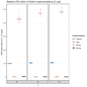
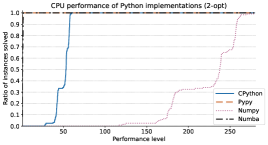
(a) 2-opt benchmark

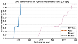
(b) Or-opt benchmark

Figure 1: Python implementations: box plots and performance profiles

The box plots indicate that the performance of the numpy implementation is always more than 400 times slower than the c++14 implementation. The performance profiles show that it is also up to 600 times slower than the fastest Python implementation in some cases. Overall, it is clear that the Numpy implementation has the worst performance. This is easily explained: every time a function from Numpy is called, it is wrapped in order to call the C code for that function. At the same time, none of the benchmarks actually use functions which would make this beneficial, i.e. functions that would perform a lot of calculations written in C then return the result of this calculation (e.g. matrix multiplication). Such operations are simply not needed in these benchmarks. Therefore the cost of calling C code is paid often, but the benefits are never reaped. Additionally, it is clear that the base CPython implementation is also very slow, although not as much as the Numpy one. However, the Numpy structures combined with JIT compilation from Numba look promising.

We now compare Pypy and Numba only, on all benchmarks except for lns and espprc, since they are not implemented with Numba as explained above. These results are presented in Figure 2.

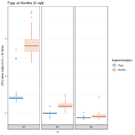
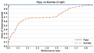
(a) 2-opt benchmark

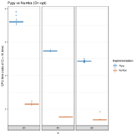
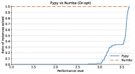
(b) Or-opt benchmark

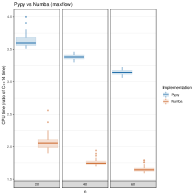
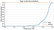
(c) maxflow benchmark

Figure 2: Pypy vs Numba: box plots and performance profiles

Pypy is up to almost twice as fast as Numba on the 2-opt benchmark, while Numba is more than three times as fast in a majority of cases for the Or-opt benchmark and up to twice as fast for the maxflow benchmark. We also note that for the 2-opt benchmark, the performance gap reduces when instance size increases, keeping in mind that the 2-opt benchmark is the fastest of the lot. This may simply mean that Numba has a higher initial cost for JIT compilation. Overall it seems that Numba is faster, except for very quick computations. However we still see two reasons to use Pypy: it does not require any modification to the Python code, and it is feature-complete, thus allowing to implement all benchmarks. In fact the code for the CPython and Pypy implementations of each benchmark is fully identical.

5.3 Impact of using a flat matrix

We now look at the impact of using a flat distance matrix representation, across multiple languages. The expectation is that it should generally be at least as fast, as long as function calls are inlined; however, in the case of languages that have multi-dimensional arrays, it is harder to predict. We first look at such a comparison for the c++14 implementation in Figure 3, considering benchmarks 2-opt and Or-Opt. Benchmarks maxflow and espprc use their own matrix structure, therefore we do not include them in this comparison.

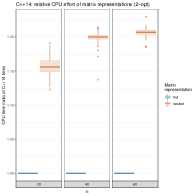
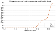
(a) 2-opt benchmark

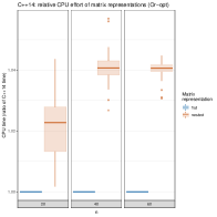
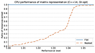
(b) Or-opt benchmark

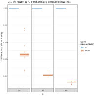
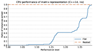
(c) lns benchmark

Figure 3: C++14: comparison of matrix representations

Although not depicted here, similar observations can be made with most languages, with the notable exception of base Python (i.e. using CPython without Numba). Since CPython does not do any kind of function inlining, the performance cost of calling functions for each distance lookup outweighs the performance benefit of using a flat, contiguous matrix representation.

We now compare a flat matrix representation in Julia against the “natural” representation using Julia’s native multi-dimensional arrays. This comparison is presented in Figure 4.

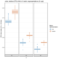
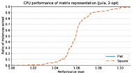
(a) 2-opt benchmark

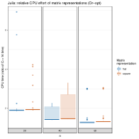
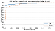
(b) Or-opt benchmark

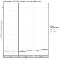
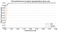
(c) lns benchmark

Figure 4: Julia: comparison of matrix representations

While it is not overwhelming, there can still be a benefit in using a flat matrix representation.

Overall, it appears that it is never a significantly bad idea to use a flat matrix representation in our setup, while it can bring benefits. Therefore, from this point on, flat matrix representation is used by default.

5.4 Impact of using static arrays

In some cases, variable-size arrays are not necessary. This is the case for example when implementing a 2-opt procedure for a TSP. In these cases, fixed-size arrays are enough and their performance have to be at least as good as the performance of variable-size arrays (like C++’s vectors). We run this comparison for benchmarks 2-opt and Or-opt, which can be both implemented easily using the fixed-size native arrays of C++, which are C native arrays, and which work in a similar fashion in Java. We run this comparison for both C++14 and Java, the results are summarized in Figure 5.

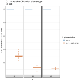
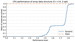
(a) C++14, 2-opt benchmark

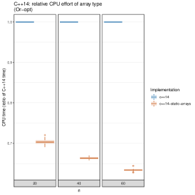
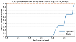
(b) C++14, Or-opt benchmark

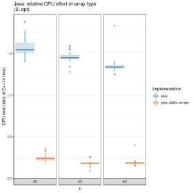
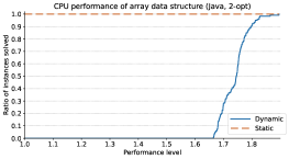
(c) Java, 2-opt benchmark

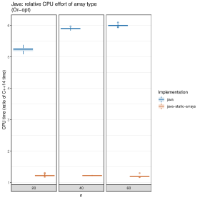
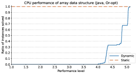
(d) Java, Or-opt benchmark

Figure 5: Performance of static arrays versus variable-size vectors.

Using static arrays in C++ can be up to almost twice as fast, while in Java it can be up to five times as fast. One possible explanation why the gap is larger in Java lies in the nature of the Java containers used: we use ArrayList objects, which take as generic parameter the class of the objects stored in the collection, e.g. ArrayList<Integer>. This parameter can only be a class, not a native type, which matters in Java. This means that it is not possible to have a collection of int variables, only a collection of Integer objects, each wrapping an int.

5.5 A comparison of C++ implementations

We investigate the difference in performance between using C++14’s smart pointers and older traditional C++ coding with references and/or C pointers. For that purpose, we compare the C++14 and C++98 implementations of each benchmark. Figure 6 summarizes this comparison.

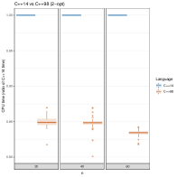
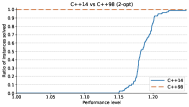
(a) 2-opt benchmark

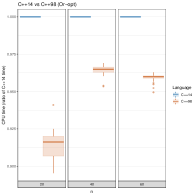
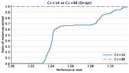
(b) Or-opt benchmark

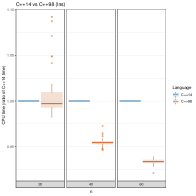
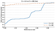
(c) lns benchmark

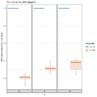
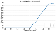
(d) espprc benchmark

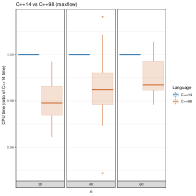
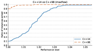
(e) maxflow benchmark

Figure 6: Performance of C++14 versus C++98.

The C++98 implementation is faster in all five benchmarks, although not always by much. We conclude that if something can be implemented in our setup without using smart pointers and without extra effort, then it is a good idea to do so.

5.6 General cross-language comparison

We now compare the performance of various programming languages when performing the same tasks. We compare the following languages: C++, Java, JavaScript, Julia, Python and Rust. For that purpose, we use what seems to be the best choice for each language based on the above experiments, meaning that we use the C++98 implementation for C++, and the Pypy interpreter when running a Python program. There is a natural separation between compiled “fast” languages (C++, Java, Julia, Rust) on one side and “interpreted” languages (Python, JavaScript) on the other side. No language is exclusively interpreted, as Pypy and Node use JIT compiling; this being said, there is a performance gap between fast and interpreted languages, and in order to produce more readable charts we compare them separately.

5.6.1 Cross-language comparison: “fast” languages

We compare the performance of fast languages in Figure 7.

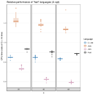
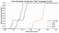
(a) 2-opt benchmark

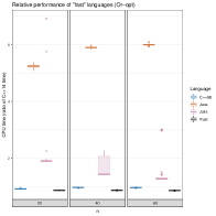
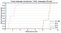
(b) Or-opt benchmark

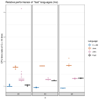
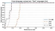
(c) lns benchmark

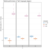
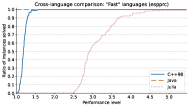
(d) espprc benchmark

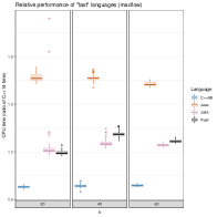
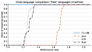
(e) maxflow benchmark

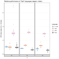
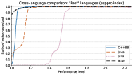
(f) espprc-index benchmark

Figure 7: Performance of “fast” languages.

There is no clear winner: each language is the fastest for at least one of the benchmarks. There are however some relatively large factors in the execution speed in some cases, up to a factor 8 in the case of Java for the Or-opt benchmark. However in many cases the factor between two languages is never more than three. This is reassuring for the researchers and students who want to use, in this setup, something else than C++ and are worried about the performance hit.

5.6.2 Cross-language comparison: “interpreted” languages

We compare the performance of interpreted languages in Figure 8.

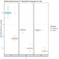
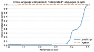
(a) 2-opt benchmark

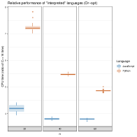
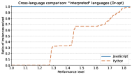
(b) Or-opt benchmark

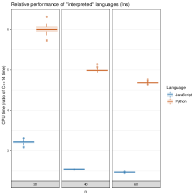
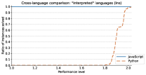
(c) lns benchmark

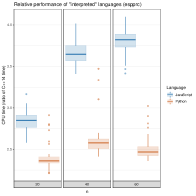
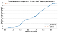
(d) espprc benchmark

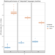
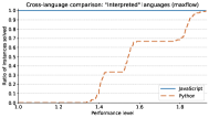
(e) maxflow benchmark

Figure 8: Performance of “interpreted” languages.

Again there is no clear winner: both Python and JavaScript offer the best performance for some of the benchmarks. More interestingly, these implementations are never slower than ten times the effort required by the baseline C++14 implementation (with the exception of one outlier for the Python implementation of the Or-opt benchmark). In many cases, they are less than five times slower even. This means that depending on the use case, implementing routing optimization algorithms in Python or JavaScript can be a viable (and convenient) option.

5.7 Cross-platform comparison

Many findings presented above can be reproduced on different platforms, however in some cases different platforms produce different outcomes. We now illustrate this with an example, looking at the comparison of Pypy and Numba on the 2-opt benchmark. We run the 2-opt benchmark on the previously mentioned Xeon CPU as well as on a Raspberry Pi 4 board with an ARMv7 CPU, 4 cores, 1.5 GHz. Pypy versions differ slightly: 7.0.0 on the ARMv7 CPU versus 7.3.3 on the Xeon CPU. The Numba version is 0.42.0 on both platforms. Figure 9 summarises and compares these runs. Ratios are computed independently for each platform, e.g. the CPU time on ARMv7 is presented as a ratio of the CPU time taken by the C++14 implementation on ARMv7.

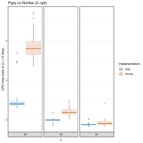
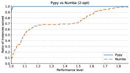
(a) Computing cluster: Intel Xeon E5-2650 v3, 20 cores, 3 GHz.

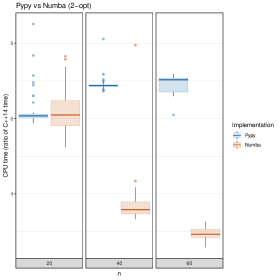
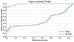
(b) Raspberry Pi 4: ARMv7, 4 cores, 1.5 GHz.

Figure 9: Pypy versus Numba on 2-opt benchmark: different platforms.

The trends are opposite on different platforms. This may be due to several reasons, for instance certain JIT compilers working better with certain CPUs, or version differences for Pypy and/or Numba. Ultimately, we emphasize that it would be unwise to generalise the observations made previously to different settings. The goal of this article is not to provide final conclusions on what tool to use, rather to introduce the BROUTE benchmark suite and encourage using it when making early design decisions on implementation, using the appropriate experimental platform to draw the appropriate conclusions.

5.8 Experiments using standard VRP instances

All instances used thus far have vertices whose coordinates are generated using a uniform distribution. We now look at the same experiments but using instances from the VRPLIB, available at http://or.dei.unibo.it/library/vrplib-vehicle-routing-problem-library, which are more diverse in terms of vertex location generation. These results are presented in Appendix C. They are largely identical to the previously observed results.

6 Discussion

The question of what programming language to use when implementing optimization algorithms is one that, by essence, does not have a final answer. This being said, there is value in knowing how much performance is gained or lost when using a certain language on a certain architecture, or how much can be gained by using different data structures. The benchmark suite introduced in this paper is free software and can be used for that purpose. We encourage students and researchers in transport optimization to use it to support their implementation decisions. Further experimental analyses, similar in flavor to the ones conducted here, can also be good practice. For instance, comparing the runtime performance of the same C++ code when compiled with different compilers may provide a speedup for very little effort.

Additionally, some insight can already be taken straight out of the experiments conducted above. Using languages like Julia or Rust does not incur a significant runtime penalty when compared to more established languages like C++, and can actually be faster sometimes. Interpreted languages like Python or JavaScript nowadays have reasonably good runtime performance, usually less than five times slower than pre-compiled languages, under the right conditions (typically, using a JIT compiler). This means that the flexibility and ease of use of these languages can be worth the performance hit, depending on the application. Additionally, using JavaScript opens perspectives, as the integration of optimization algorithms in web applications is easier than it ever was, and these algorithms can now be run efficiently client-side.

This is only the initial version of BROUTE; contributions are encouraged, concerning both languages and algorithms. For example a Matlab or C# implementation of all benchmark algorithms would be welcome as long as they can be run for free under the main operating systems. Implementing a new benchmark in all currently supported languages would also be welcome, or even re-implementing current benchmark algorithms in currently supported languages but with different data structures.

Declarations

Conflicts of interest:

On behalf of all authors, the corresponding author states that there is no conflict of interest.

Availability of data and material:

All data sets introduced in this paper are licensed under the GNU General Public License version 3 and available at https://github.com/fa-bien/broute.

Code availability:

All code introduced in this work is licensed under the GNU General Public License version 3 and available at https://github.com/fa-bien/broute. This includes the code to generate the charts.

Appendix A Summary of languages and versions

Language/tool	language or compiler version	options
C++14	g++ 8.3.0	-Wall -ansi -pedantic -O3 -std=c++14
C++98	g++ 8.3.0	-Wall -ansi -pedantic -O3 -std=c++98
CPython	3.7.3
Pypy	7.3.3-beta0
Numpy	1.16.2
Numba	0.42.0
Java	OpenJDK version 11
Julia	1.6.0	–check-bounds=no –inline=yes -O3 -t 1
Rust	1.51	cargo build –release
JavaScript	Node v14.15.4

Table 1: Overview of languages and versions.

Appendix B Pseudocode for each benchmark algorithm

We use square braces to indicate array/vector indices, starting at index 0, while $[]$ represents a new empty array/vector and $length(x)$ is the number of elements in array $x$. Function $push(x,e)$ is used to append value $e$ to array $x$. Function $delete(x,i)$ deletes, in array $x$, the element at index $i$; function $insert(x,i,v)$ inserts value $v$ at index $i$ in array $x$, shifting values at index $i$ and beyond to the right. Functions $delete()$ and $insert()$ have linear worst-case time complexity.

In what follows, $n$ is the number of vertices in the distance matrix and auxiliary graphs, $d_{ij}$ is the distance between two vertices $i$ and $j$, while $s$ represents the seed solution. In algorithms performing local search (2-opt, Or-opt, lns), this seed represents the initial solution. In other algorithms (espprc, maxflow), it is used to generate the respective instance.

B.1 2-opt

The 2-opt benchmark is outlined in algorithm 1. It relies on function $first2eimprovement(s)$, which looks for an improving 2-exchange in solution $s$. If it finds one, it performs it (with a side effect on $s$) and returns $true$; otherwise it returns $false$. The total number of improvements performed is returned.

Algorithm 1 $2-opt(s)$

1:  $t\leftarrow 0$

2:  while $first2eimprovement(s)$ do

3:     $t\leftarrow t+1$

4:  end while

5:  return  $t$

Algorithm 2 $first2eimprovement(s)$

1:  for $p_{1}\in\{1..|s|-3\}$ do

2:     for $p_{2}\in\{p_{1}+1..|s|-1\}$ do

3:        if $d_{s[p_{1}],s[p_{1}+1]}+d_{s[p_{2}],s[p_{2}+1]}>d_{s[p_{1}],s[p_{2}]}+d_{s[p_{1}+1],s[p_{2}+1]}$ then

4:           for $i\in\{0..\lfloor\frac{p_{2}-p_{1}+1}{2}\rfloor\}$ do

5:              $s[p_{1}+1+i]\leftrightarrow s[p_{2}-i]$

6:           end for

7:           return  $true$

8:        end if

9:     end for

10:  end for

11:  return  $false$

B.2 Or-opt

The Or-opt benchmark follows a similar pattern as the 2-opt one. Algorithm 3 outlines it.

Algorithm 3 $Or-opt(s)$

1:  $t\leftarrow 0$

2:  while $firstorimprovement(s)$ do

3:     $t\leftarrow t+1$

4:  end while

5:  return  $t$

Algorithm 4 $firstorimprovement(s)$

1:  for $i\in\{1..|s|-1\}$ do

2:     for $l\in\{1..1+min(3,|s|-1-i\}$ do

3:        for $p\in\{0..i-1\}\cup\{i+l..|s|-1\}$ do

4:           $\delta\leftarrow d_{s[i-1],s[i+l]}+d_{s[p],s[i]}+d_{s[i+l-1],s[p+1]}-d_{s[p],s[p+1]}-d_{s[i-1],s[i]}-d_{s[i+l-1],s[i+l]}$

5:           if $\delta<0$ then

6:              $t\leftarrow s[i..i+l]$

7:              if $i<p$ then

8:                 $s[i..p-l+1]\leftarrow s[i+l..p+1]$

9:                 $s[p+1-l..p+1]\leftarrow t$

10:              else

11:                 $s[p+l..i-1+l]\leftarrow s[p..i-1]$

12:                 $s[p+1..p+1+l]\leftarrow t$

13:              end if

14:              return  $true$

15:           end if

16:        end for

17:     end for

18:  end for

19:  return  $false$

B.3 lns

The lns benchmark destroys then repairs the solution $niter$ times and returns, as checksum value, the sum of the costs of all insertions performed over its whole run. It is outlined in algorithm 5.

Algorithm 5 $lns(s,niter)$

1:  $checksum\leftarrow 0$

2:  for $iter\in\{1..niter\}$ do

3:     $tmp\leftarrow copy(s)$

4:     $unplanned\leftarrow[]$

5:     $where\leftarrow 1$

6:     while $where<length(tmp)-1$ do

7:        $push(unplanned,tmp[where])$

8:        $delete(tmp,where)$

9:        $where\leftarrow where+1$

10:     end while

11:     while $length(unplanned)>0$ do

12:        $bc,bn,bf,bt\leftarrow\infty,-1,-1,-1$

13:        for $p_{1}\in\{0..unplanned\}$ do

14:           $k\leftarrow unplanned[p_{1}]$

15:           for $p_{2}\in\{0..|tmp|-1\}$ do

16:              $i,j\leftarrow tmp[p],tmp[p+1]$

17:              $\delta\leftarrow d_{ik}+d_{kj}-d_{ij}$

18:              if $\delta<bc$ then

19:                 $bc\leftarrow\delta$

20:                 $bn,bf,bt\leftarrow k,p_{1},p_{2}$

21:              end if

22:           end for

23:        end for

24:        $insert(tmp,bt+1,bn)$

25:        $delete(unplanned,bf)$

26:        $checksum\leftarrow checksum+bc$

27:     end while

28:     $s\leftarrow tmp$

29:  end for

30:  return  $checksum$

B.4 maxflow

For the sake of legibility, the generation of the maxflow instances is not described here. In order to solve one maxflow instance, we need two auxiliary graphs: one to store capacities and one to store flow values. To represent these two graphs we use two arrays. These arrays must be allocated in memory once when reading the input data, before the timing of the benchmark starts, then reused for each separate instance. Hence the memory allocation of auxiliary graphs is not timed, however filling it with values for a given seed is included in the time for the benchmark (but not represented below). Function $edmondskarp(C,F,s,t)$ computes the maximum flow from source $s$ to sink $t$ in a graph of $n$ vertices where capacities are provided in array $C$, and flows are stored in array $F$. $F$ is pre-allocated but needs to be initialized to zero values. Both $C$ and $F$ are nested arrays or multi-dimensional arrays depending on what the language allows. $Q$ is a first-in-first-out (FIFO) queue. Function $pop(Q)$ removes the first element in $Q$ and returns it.

Algorithm 6 $edmondskarp(C,F,s,t)$

1:  $totalflow\leftarrow 0$

2:  $moreflow\leftarrow true$

3:  $Q\leftarrow\emptyset$

4:  $pred\leftarrow$ array of size $n$

5:  for $i\in\{0..n-1\}$ do

6:     for $j\in\{0..n-1\}$ do

7:        $F[i,j]\leftarrow 0$

8:     end for

9:  end for

10:  while $moreflow$ do

11:     for $i\in\{0..n-1\}$ do

12:        $pred[i]\leftarrow-1$

13:     end for

14:     $push(Q,s)$

15:     while $length(Q)>0$ do

16:        $c\leftarrow pop(Q)$

17:        for $j\in\{0..n-1\}$ do

18:           if $j\neq c\land pred[j]=-1\land j\neq s\land C[c,j]>F[c,j]$ then

19:              $pred[j]\leftarrow c$

20:              $push(Q,j)$

21:           end if

22:        end for

23:     end while

24:     if $pred[t]\neq-1$ then

25:        $df\leftarrow\infty$

26:        $i,j\leftarrow pred[t],t$

27:        while $i\neq-1$ do

28:           if $df>C[i,j]-F[i,j]$ then

29:              $df\leftarrow C[i,j]-F[i,j]$

30:           end if

31:           $i,j\leftarrow pred[i],i$

32:        end while

33:        $i,j\leftarrow pred[t],t$

34:        while $i\neq-1$ do

35:           $F[i,j]\leftarrow F[i,j]+df$

36:           $i,j\leftarrow pred[i],i$

37:        end while

38:        $totalflow+=df$

39:     else

40:        $moreflow\leftarrow false$

41:     end if

42:  end while

43:  return  $totalflow$

B.5 espprc

Similar to maxflow, we only provide the pseudocode to solve one instance of espprc. Also similar to maxflow, the auxiliary graph, used this time to store the reduced cost of each arc, is only allocated once and this allocation is not timed. Let $rc$ be the auxiliary graph (matrix) containing reduced costs, $nres$ the number of resources considered, $C$ the capacity for each resource, $q_{ir}$ the resource consumption for vertex $i$ and resource $r$ (0 or 1), and $M$ the maximum length a tour may have. Function $esprrc(rc,nres,C,q,M)$ computes all shortest paths from vertex 0 to itself which are elementary except for the two visits at node 0, do not consume more resources than $C$ for any resource, and do not exceed length $M$. Note that given the definition of resource consumption provided in Section 2.4, $q_{ir}$ can be inlined using bit operations, and that is the case in every implementation. Function $espprc()$ is outlined in Algorithm 7. Similar to the maxflow algorithm, $Q$ is a FIFO queue. Function $espprc()$ relies on labels, each label containing the following attributes for a partial path:

• $cost$: total cost according to reduced cost matrix $rc$.

• $length$: total length according to distance matrix $d$.

• $visited$: set of nodes that are already visited.

• $predecesor$: predecessor label (for path reconstruction).

• $successors$: collections of successor labels (for recursive marking in case this label is found to be dominated).

• $q$ : resource consumption for each resource (index with $r$).

• $marked$: boolean flag determining whether a label is marked to be ignored.

In the following we consider that these attributes can be accessed using the dot operator, e.g. $l.length$ is the length of label $l$. We perform the following operations with such labels:

• $emptylabel()$: create an empty label.

• $extend(l,v)$: extend label $l$ to vertex $v$.

• $updatedominance(l,nl)$: compare a new label $nl$ against a collection $l$ of labels, all representing a path to the same vertex. If $nl$ is dominated by at least one element of $l$, return $false$. Otherwise, add $nl$ to $l$, marking all elements of $l$ that are dominated by $nl$, and return $true$. No label is deleted during the algorithm, instead they are marked to be ignored. Memory is only freed after the algorithm has converged.

For the sake of legibility, we do not detail these label operations here. Moreover, they are typically heavily language-dependent.

Algorithm 7 $espprc(rc,nres,C,q,M$

1:  $Q\leftarrow$

2:  $labels\leftarrow$ array of empty arrays, one per vertex

3:  $push(labels[0],emptylabel())$

4:  while $Q\neq\emptyset$ do

5:     $c\leftarrow pop(Q)$

6:     for $l\in labels[c]$ do

7:        if $\lnot l.marked$ then

8:           for $succ\in\{0..n-1\}$ do

9:              if $succ\in l.visited\lor succ=c\lor l.length+d_{n,succ}+d_{succ,0}>M$ then

10:                 continue (skip remainder of this iteration of the loop)

11:              end if

12:              $rfeas\leftarrow true$

13:              for $r\in\{1..nres\}$ do

14:                 if $q_{succ,r}>0\land l.q_{r}+1>C$ then

15:                    $rfeas\leftarrow false$

16:                    break (exit this loop)

17:                 end if

18:              end for

19:              if $\lnot rfeas$ then

20:                 continue

21:              end if

22:              $nl\leftarrow extend(l,succ)$

23:              $added\leftarrow updatedominance(labels[succ],nl)$

24:              if $added$ then

25:                 $push(l.successors,nl)$

26:                 if $succ\notin Q\land succ\neq 0$ then

27:                    $push(Q,succ)$

28:                 end if

29:              end if

30:           end for

31:        end if

32:     end for

33:  end while

34:  return  minimum cost among all labels at vertex $0$

Appendix C Experimental results on VRPLIB instances

We conduct experiments on instances from the VRPLIB, which can be found at http://or.dei.unibo.it/library/vrplib-vehicle-routing-problem-library. We use the symmetric CVRP instances, ignoring vehicle capacity. These instances use Euclidean distance but vertex coordinates are not randomly generated with a uniform distribution like our instances. Some of these instances use the same distance matrix; we consider a maximal subset of VRPLIB instances with unique distance matrices. They are summarized in Table 2.

Instance	# vertices
E016-03m	16
E021-04m	21
E022-04g	22
E023-03g	23
E026-08m	26
E030-03g	30
E031-09h	31
E033-04g	33
E036-11h	36
E041-14h	41
E045-04f	45
E048-04y	48
E051-05e	51
E072-04f	72
E076-07s	76
E076A10r	76
E076B09r	76
E076C09r	76
E076D09r	76

Table 2: VRPLIB instances

For each instance we generate 1000 starting seeds randomly, as previously. The variations in instance size do not allow to group them by size conveniently, which is what we used for box plots. Therefore we only report performance profiles here. We produce the same figures as 1 – 8 from Section 5, in the same order, in figures 10 – 17. We omit the cross-platform comparison as it is of limited interest here.

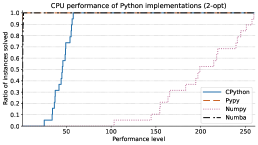
(a) 2-opt benchmark

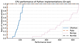
(b) Or-opt benchmark

Figure 10: Python implementations: performance profiles (VRPLIB)

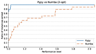
(a) 2-opt benchmark

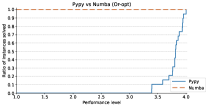
(b) Or-opt benchmark

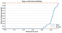
(c) maxflow benchmark

Figure 11: Pypy vs Numba: performance profiles (VRPLIB)

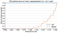
(a) 2-opt benchmark

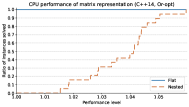
(b) Or-opt benchmark

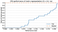
(c) lns benchmark

Figure 12: C++14: comparison of matrix representations (VRPLIB)

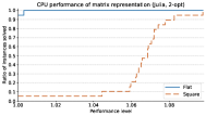
(a) 2-opt benchmark

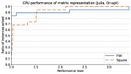
(b) Or-opt benchmark

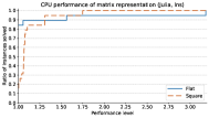
(c) lns benchmark

Figure 13: Julia: comparison of matrix representations (VRPLIB)

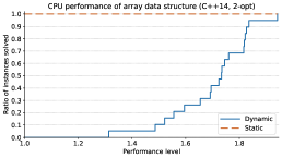
(a) C++14, 2-opt benchmark

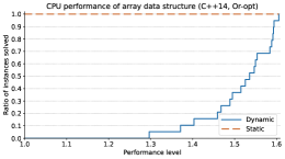
(b) C++14, Or-opt benchmark

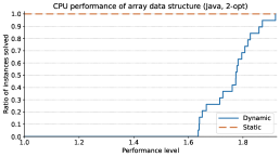
(c) Java, 2-opt benchmark

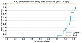
(d) Java, Or-opt benchmark

Figure 14: Performance of static arrays versus variable-size vectors (VRPLIB)

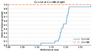
(a) 2-opt benchmark

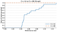
(b) Or-opt benchmark

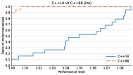
(c) lns benchmark

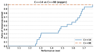
(d) espprc benchmark

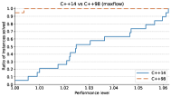
(e) maxflow benchmark

Figure 15: Performance of C++14 versus C++98 (VRPLIB)

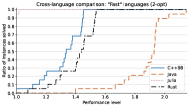
(a) 2-opt benchmark

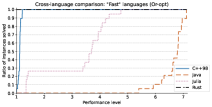
(b) Or-opt benchmark

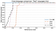
(c) lns benchmark

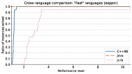
(d) espprc benchmark

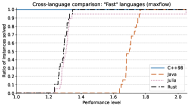
(e) maxflow benchmark

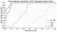
(f) espprc-index benchmark

Figure 16: Performance of “fast” languages (VRPLIB)

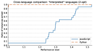
(a) 2-opt benchmark

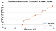
(b) Or-opt benchmark

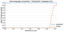
(c) lns benchmark

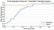
(d) espprc benchmark

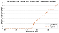
(e) maxflow benchmark

Figure 17: Performance of “interpreted” languages (VRPLIB)

Since there are less instances as in the previous experiments, the steps in performance profiles are more noticeable: there are 19 instances here, so each profile has at most 19 steps. The trends are the same as before. The comparison of fast languages on the espprc benchmark looks a bit different but is in fact very similar, except it is stretched horizontally due to one unusually longer Julia run. Overall, it appears that the way the distance matrix is generated does not impact the relative runtime budget required by the different implementations.

References

- Baldacci et al., (2012) Baldacci, R., Mingozzi, A., and Roberti, R. (2012). Recent exact algorithms for solving the vehicle routing problem under capacity and time window constraints. European Journal of Operational Research, 218(1):1 – 6.
- Bezanson et al., (2017) Bezanson, J., Edelman, A., Karpinski, S., and Shah, V. B. (2017). Julia: A fresh approach to numerical computing. SIAM Review, 59(1):65–98.
- Cacchiani et al., (2014) Cacchiani, V., Hemmelmayr, V. C., and Tricoire, F. (2014). A set-covering based heuristic algorithm for the periodic vehicle routing problem. Discrete Applied Mathematics, 163:53–64.
- Croes, (1958) Croes, G. (1958). A method for solving traveling-salesman problems. Operations Research, 6(6):791–908.
- Dolan and Moré, (2002) Dolan, E. D. and Moré, J. J. (2002). Benchmarking optimization software with performance profiles. Mathematical Programming, 91(2):201–213.
- Edmonds and Karp, (1972) Edmonds, J. and Karp, R. M. (1972). Theoretical improvements in algorithmic efficiency for network flow problems. Journal of the ACM, 19(2):248–264.
- Feillet et al., (2004) Feillet, D., Dejax, P., Gendreau, M., and Gueguen, C. (2004). An exact algorithm for the elementary shortest path problem with resource constraints: Application to some vehicle routing problems. Networks, 44(3):216–229.
- Ford and Fulkerson, (1956) Ford, L. R. and Fulkerson, D. R. (1956). Maximal flow through a network. Canadian Journal of Mathematics, 8:399–404. Publisher: Cambridge University Press.
- GitHub, (2020) GitHub (2020). The 2020 state of the octoverse. https://octoverse.github.com/. [Online; accessed 17-Feb-2021].
- Harris et al., (2020) Harris, C. R., Millman, K. J., van der Walt, S. J., Gommers, R., Virtanen, P., Cournapeau, D., Wieser, E., Taylor, J., Berg, S., Smith, N. J., Kern, R., Picus, M., Hoyer, S., van Kerkwijk, M. H., Brett, M., Haldane, A., del R’ıo, J. F., Wiebe, M., Peterson, P., G’erard-Marchant, P., Sheppard, K., Reddy, T., Weckesser, W., Abbasi, H., Gohlke, C., and Oliphant, T. E. (2020). Array programming with NumPy. Nature, 585(7825):357–362.
- Helsgaun, (2000) Helsgaun, K. (2000). An effective implementation of the lin–kernighan traveling salesman heuristic. European Journal of Operational Research, 126(1):106–130.
- Helsgaun, (2009) Helsgaun, K. (2009). General k-opt submoves for the lin–kernighan tsp heuristic. Mathematical Programming Computation, 1(2):119–163.
- Hunter, (2007) Hunter, J. D. (2007). Matplotlib: A 2d graphics environment. Computing in Science & Engineering, 9(3):90–95.
- Julia Documentation, (2021) Julia Documentation (2021). Performance tips. https://docs.julialang.org/en/v1/manual/performance-tips/. [Online; accessed 11-Feb-2021].
- JunoLab, (2020) JunoLab (2020). Traceur. https://github.com/JunoLab/Traceur.jl. [Online; accessed 11-Feb-2021].
- nodejs.org, (2021) nodejs.org (2021). Node.js. https://nodejs.org.
- Or, (1976) Or, I. (1976). Traveling salesman-type combinatorial problems and their relation to the logistics of regional blood banking. PhD thesis, Department of Industrial Engineering and Management Sciences, Northwestern University, Evanston, IL.
- Oracle Corporation, (2011) Oracle Corporation (2011). Moving to openjdk as the official java se 7 reference implementation. https://blogs.oracle.com/java/moving-to-openjdk-as-the-official-java-se-7-reference-implementation. [Online; accessed 10-Feb-2021].
- Padberg and Rinaldi, (1987) Padberg, M. and Rinaldi, G. (1987). Optimization of a 532-city symmetric traveling salesman problem by branch and cut. Operations Research Letters, 6(1):1–7.
- Pisinger and Ropke, (2010) Pisinger, D. and Ropke, S. (2010). Large Neighborhood Search, pages 399–419. Kluwer’s International Series.
- Pypy, (2021) Pypy (2021). Pypy. https://pypy.org. [Online; accessed 17-Feb-2021].
- R Core Team, (2021) R Core Team (2021). R: A Language and Environment for Statistical Computing. R Foundation for Statistical Computing, Vienna, Austria.
- Sadykov and Vanderbeck, (2021) Sadykov, R. and Vanderbeck, F. (2021). Bapcod — a generic branch-and-price code. Technical report, Inria Bordeaux Sud-Ouest HAL-03340548.
- Shaw, (1998) Shaw, P. (1998). Using constraint programming and local search methods to solve vehicle routing problems. In Principles and Practice of Constraint Programming - CP98, pages 417–431. Springer-Verlag.
- Taillard and Helsgaun, (2019) Taillard, E. D. and Helsgaun, K. (2019). Popmusic for the travelling salesman problem. European Journal of Operational Research, 272(2):420–429.
- The Rust Team, (2021) The Rust Team (2021). Rust. https://rust-lang.org. [Online; accessed 18-Feb-2021].
- TIOBE, (2020) TIOBE (2020). Tiobe programming community index definition. https://www.tiobe.com/tiobe-index/programming-languages-definition/. [Online; accessed 17-Feb-2021].
- TOP500, (2021) TOP500 (2021). Top500. https://top500.org/. [Online; accessed 17-Feb-2021].
- Vidal, (2016) Vidal, T. (2016). Technical note: Split algorithm in o(n) for the capacitated vehicle routing problem. Computers & Operations Research, 69:40–47.
- Wickham, (2016) Wickham, H. (2016). ggplot2: Elegant Graphics for Data Analysis. Springer-Verlag New York.