Functorial String Diagrams for Reverse-Mode Automatic Differentiation

Abstract.

We enhance the calculus of string diagrams for monoidal categories with hierarchical features in order to capture closed monoidal (and cartesian closed) structure. Using this new syntax we formulate an automatic differentiation algorithm for (applied) simply typed lambda calculus in the style of (DBLP:journals/toplas/PearlmutterS08) and we prove for the first time its soundness. To give an efficient yet principled implementation of the AD algorithm we define a sound and complete representation of hierarchical string diagrams as a class of hierarchical hypergraphs we call hypernets.

1. Introduction

This paper covers three main topics which support, motivate, and reinforce each other: reverse automatic differentiation (AD), string diagrams, and (hyper)graph rewriting.

AD is an established technique for evaluating the derivative of a function specified by a computer program, a particularly challenging exercise when the program contains higher-order sub-terms. This technique came to recent prominence due to its important role in algorithms for machine learning (DBLP:journals/jmlr/BaydinPRS17). We focus in particular on the influential algorithm defined in (DBLP:journals/toplas/PearlmutterS08), which lies at the foundation of many practical implementations of AD. The main novel contribution of our paper is to prove, for the first time, the soundness of this particular style of AD algorithm.

String diagrams are a formal graphical syntax used in the representation of morphisms in monoidal categories (selinger2010survey) which is finding an increasing number of applications in a wide range of mathematical, physical, and engineering domains. We contribute to the development of string diagrams by formulating a new hierarchical string diagram calculus, with associated equations, suitable for the representation of closed monoidal (and cartesian closed) structures. This innovation is, as we shall see in the paper, warranted: the hierarchical string diagrammatic syntax allows for a more intelligible formulation of a complex algorithm and, most importantly, a new style of inductive argument which leads to a relatively simple proof of soundness.

Finally, hierarchical hypergraphs are given as a concrete and efficient representation of hierarchical string diagrams, which pave the way towards efficient and effective implementation of AD as graph rewriting in the well established framework of double-pushout (DPO) rewriting (DBLP:conf/mfcs/EhrigK76). Moreover, we identify a class of hierarchical hypergraphs, which we call hypernets, which are a sound and complete representation of the hierarchical string diagram calculus. This is the third and final contribution of our paper.

2. Higher-order string diagrams

String diagrams are a convenient alternative notation for constructing morphisms, in particular in (strict) monoidal categories. In this paper we largely build on the syntax proposed in (DBLP:conf/csl/Mellies06), with only a few cosmetic changes aimed at making higher-order concepts more perspicuous. String diagrams in this work are to be read from top to bottom.

2.1. Functorial string diagrams

We start with the basic language of categories, ranged over by $\mathcal{C},\mathcal{D}\ldots$. This language consists of a collection of objects ranged over by $A,B,\ldots$ and two families of terminal symbols, identities $\text{id}_{A}:A\to A$, represented as an $A$-labelled vertical stem  , and morphisms $f:A\to B$, represented by labelled boxes with an $A$-labelled top stem (which we sometimes call input or operand) and a $B$-labelled bottom stem (which we call output or result)  . We may distinguish (families of) terminal symbols in the diagram language with particular geometrical shapes instead of labelled boxes, much in the way we have artificially disgtinguished identities from other morphisms.

Terms, ranged over by $f,g,\ldots$, are created using composition. Given $f:A\to B$, and $g:B\to C$ we write $f;g:A\to C$ as the stacking of the diagrams for $f$ and $g$. Since the output of $f$ must match the input of $g$ we connect the corresponding stems, to give a graph-like appearance to the string diagram  . We enforce two properties of composition familiar from category theory. First, composition is associative, meaning $(f;g);h=f;(g;h)=f;g;h$. This identification is subsumed by the diagrammatic notation. Second, we require the identity axiom $f;\text{id}=\text{id};f=f$. Diagrammatically, this means the lengths of the stems of a diagram can be lengthened or shortened without ambiguity.

Figure 1. An example frame

We extend our string diagram language with labelled frames which indicate mappings between morphisms of different categories. The application of a mapping $F$ to a morphism, as a string diagram, is indicated by drawing an $F$-labelled frame around the morphism and modifying the stems of the diagram as appropriate, as seen in Fig. 1. Note that in this diagram the stems and morphims inside the frame are a different color to the frame and the stems outside the frame. This is an indication that objects and morphisms belong to potentially distinct categories. When the map goes from a category to itself, we may use the same color inside and out of the frame, but often leave the frame itself a different color to emphasize the mapping.

Such morphism mapping $F$ constitutes a functor if it satisfies the following properties. First, there must be a mapping on objects, which we also denote $F$ by common abuse of notation, such that $F_{i}(f)=F(A)$ and $F_{o}(f)=F(B)$ for all $f:A\to B$ in the source category. Second, this mapping must respect basic categorical structures, expressed in the language of string diagrams in Fig. 2. We use $1_{\mathcal{C}}$ for the identity functor. Given two functors $F,G$ with matching domains and codomains we write $FA=F(A)$ and $FGA=F(G(A))$ in the sequel.

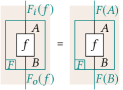
(a) Uniform on inputs and outputs

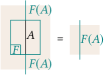
(b) Respect identity

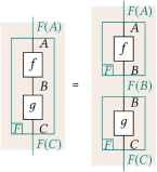
(c) Respect composition

Figure 2. Properties of functors

The diagrammatic notation can be generalised to bifunctors in the obvious way, by drawing two side-by-side boxes for the arguments. One bifunctor that plays a special role in string diagram is the tensor product or monoidal product, in particular when it is strict. The tensor is represented diagrammatically as:

= =

The diagram above contains three representations. In the first one we can see tensor as a bifunctor, with the two separate boxes indicating the two arguments of the bifunctor. The second one is special notation for the tensor, essentially hiding the functorial box and using a graphical convention (the horizontal line) to represent the ‘unravelling’ of the tensored-labelled stem into components. Finally, the third one is special notation for strict monoidal tensor, in which the tensor $A\otimes C$ is represented as the list of its components $[A,C]$. The strict diagram absorbs the associativity isomorphisms and makes the tensor associative on the nose:

= =

Henceforth we will work in the strict setting, but it will be sometimes convenient to de-strictify a diagram and group individual stems in stems with tensor types. Coherence (and strictness) ensure that such de-strictifiations can be always performed unambiguously.

In the strict setting we also have special notation for the unit $I$ of the tensor, which we represent as the empty list; identity on $I$ is represented as empty space. It is immediate then, diagrammatically, that $f\otimes\text{id}_{I}=\text{id}_{I}\otimes f=f$.

We further extend the string diagram with the concept of natural transformation between functors with the same domains and same codomains. Natural transformations are object-indexed families of morphisms written as $\theta_{A}:FA\to GA$ (or just $\theta:F\to G$) which obey the following family of axioms, expressed in the language of string diagrams as:

=

One particularly interesting example of natural transformation is symmetry, written as $\gamma_{A,B}:A\otimes B\to B\otimes A$, for which we use the special geometric shape of two crossing wires. The fact that it is a natural transformation immediately imples that

Symmetry is also an involution, i.e. $\gamma_{A,B};\gamma_{B,A}=\text{id}_{A}\otimes\text{id}_{B}$.

For functors $F:\mathcal{D}\to\mathcal{C}$ and $G:\mathcal{C}\to\mathcal{D}$ such that natural transformations $\epsilon:FG\to 1_{\mathcal{C}}$ (called the counit), $\eta:1_{\mathcal{D}}\to GF$ (called the unit) exist, they form an adjunction if and only if they satisfy the following family of axioms:

For all and we have that and .

In this situation, we say $F$ is a left adjoint and $G$ is the right adjoint.

We adopt the convention of writing the counit of an adjunction as a downward pointing semicircle, the unit as an upward pointing semicircle, and omitting the label when the map is clear from context. Note that (DBLP:conf/csl/Mellies06) does not discuss adjunctions specifically, although the streamling of the notations and calculations with adjunctions is a prime benefit of the string diagram notation, and no additional technical content is required.

2.2. String diagrams for monoidal-closed and cartesian-closed categories

Monoidal closed categories and cartesian closed categories are categorical models for the linear and simply-typed lambda calculus, respectively. A monoidal closed category arises if for every object $X$ in the category, the (endo)functor $F_{X}(A)=A\otimes X$ has a right adjoint $G_{X}(A)=X\multimap A$. Diagrammatically, we depict these functors as:

and  

Instantiated to the families of functors $F_{X},G_{X}$ above, the naturality and adjunction equations are expressed in string diagrams as in Fig. 3. The counit of the adjunction is normally called eval, and we call the unit coeval for the sake of symmetry in terminology and by analogy with compact-closed categories.

    

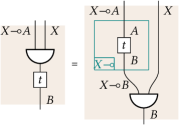
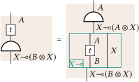
(a) Eval and coeval are natural transformations

    

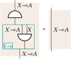
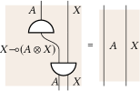
(b) Eval and coeval form an adjunction

Figure 3. String diagram representation of MCC axioms.

To further expand our diagrammatic language to cartesian closed categories, one easy way is to add natural transformations $\delta_{A}:A\to A\otimes A$ (contraction) and $\omega_{A}:A\to I$ (weakening) such that $\delta_{A};\omega_{A}\otimes\text{id}_{A}=\text{id}_{A}=\delta_{A};\omega_{A}\otimes\text{id}_{A}$ (heunen2012lectures). We represent both of these natural transformations with a black dot, disambiguated by the quantity of results. The monoid equations are  . Copying and discarding are both consequences of naturality, i.e.  and  , respectively.

Here we have presented adjunctions with unit and counit natural transformations. An equivalent description of adjunctions involves a natural bijection between sets of morphisms. In the case of monoidal or cartesian closed categories, this bijection is between ${\mathcal{C}}(\Gamma\otimes A,B)$ and ${\mathcal{C}}(\Gamma,A\multimap B)$. This bijection is known as “currying”, and is a more germane presentation for the lambda calculus. We define abstraction, the composition of the unit of the adjunction with the functorial box for $G$, as syntactic sugar denoted by a plain box with rounded corners.

$:=$

This structure for abstraction gives our notion of a hierarchical string diagram, which is to say a string diagram which may contain other string diagrams in these boxes.

2.2.1. Foliations

Terms written as string diagrams can be presented in a particular form, which will turn out to lead to some useful insights:

Definition 2.1 (Foliations).

A foliation is a string diagram written as the sequential composition of a list of diagrams called leafs. A singleton leaf is a diagram consisting of a non-identity atomic string diagram (symmetry, evaluation, operation, contraction, or weakening) or an abstraction, tensored with any number of identities. A maximally sequential foliation is a foliation comprising only singleton leafs. A maximally sequential hierarchical foliation is a maximally sequential foliation which is either abstraction free, or in which all abstracted diagrams are also maximally sequential hierarchical foliations.

For instance, if $f,g$ are not identities then the maximally sequential foliations of $f\otimes g$ are $(f\otimes id);(id\otimes g)$ and $(id\otimes g);(f\otimes id)$. The following is an obvious generalisation of a folklore theorem about monoidal categories.

Lemma 2.2.

Any hierarchical string diagram can be written as a (non-unique) maximally sequential hierarchical foliation.

The proof is straightforward. The graphical intuition which underlies the proof is that whenever two morphisms are “level” in a diagram one of them can be “shifted” using identities, then tensors and compositions can be reorganised using the functorialty of the tensor.

Foliations are convenient because syntactic transformations can be presented recursively on the foliation. This spares us the need to define ‘big’ rules for sequential and tensorial composition. Instead only ‘small’ rules for composing a term with a singleton leaf are required. This makes transformations easier to specify, and also makes for simpler inductive proofs, using the foliation as a list.

2.3. Explicit substitution in string diagrams

In this section we illustrate the use of hierarchical string diagrams to represent the simply typed lambda calculus with explicit substitutions. This is an interesting example in its own right, but more importantly it sets the scene for the next section, where we define an automatic differentiation algorithm. The explicit substitutions play an essential role, as they give us a handle on managing closures, which the AD algorithm requires.

Hierarchical string diagrams with rules for copying and discarding are a ready-made graphical syntax for the lambda calculus with explicit substitutions (DBLP:journals/jfp/AbadiCCL91). Syntactically, these calculi fall mainly in two categories, those using deBruijn indices or those using named variables. The former have better formal properties and their formalisation can be mechanised, but are not a very human-readable notation. The latter are easier to read but have some subtle failures of alpha equivalence. Formalising alpha equivalence for calculi of explicit substitution is a somewhat tricky problem, the solution of which leads back to rather intricate notations (DBLP:journals/iandc/FernandezG07). String diagrams thus seem like an improved syntax for explicit substitutions, as they are both formal and, we contend, rather readable. The graphical notation is variable-free therefore alpha equivalence is not an issue, and other equational properties are also rendered obvious by the diagrammatic representation.

We pick for comparison a presentation of the calculus of explicit substitutions with named variables (DBLP:conf/csl/Kesner07), leaving aside alpha equivalence. A $\Lambda$es-term is inductively defined as a variable $x$, an application $t\ u$, an abstraction $\lambda x.t$ or a substituted term $t[x/u]$, where $t$ and $u$ are $\Lambda$es-terms and $x$ a variable. The terms $\lambda x.t$ and $t[x/u]$ both bind $x$ in $t$. The set of free variables of a term $t$, denoted $\overline{t}$ is defined as usual.

Note that the syntactic object $[x/u]$, an explicit substitution, is not a term because of the way variable $x$ is bound. By contrast, in deBruijn formulations of the lambda calculus with explicit substitutions, substitutions are terms.

The following key equations and reduction rules are considered:

(CE) $$t[x/u][y/v] =t[y/v][x/u] y\not\in\overline{u}\land x\not\in\overline{v}$$

(BR) $$(\lambda x.t)u \rightarrow t[x/u]$$

(Var) $$x[x/u] \rightarrow u$$

(Gc) $$t[x/u] \rightarrow t x\not\in\overline{t}$$

(App) $$(t\ u)[x/v] \rightarrow t[x/v]\ u[x/v]$$

(Lamb) $$(\lambda y.t)[x/v] \rightarrow\lambda y.t[x/v] x\neq y$$

(Comp) $$t[x/u][y/v] \rightarrow t[x/u[y/v]]$$

We qualify these as ‘key’ because for more precise resource analysis the (Lamb) and (Comp) rewrites usually are given ‘linear’ forms depending on whether the substituted variable occurs in the term or not. For our purposes here we can assume the linear versions are subsumed by the general version and the (Gc) axiom.

(a) $\llbracket\Gamma\vdash tu{:}B\rrbracket$

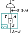
(b) $\llbracket\Gamma\vdash\lambda x.t{:}A\multimap B\rrbracket$

(c) $\llbracket\Gamma\vdash t[u/x]{:}B\rrbracket$

Figure 4. Interpretation of $\Lambda$es-terms

The string diagram interpretation of $\Lambda$es is given in Fig. 4. The proof of soundness is a straightforward exercise. Some of the axioms are simply instances of the identity (Var), associativity of composition (Comp), and naturality of the contraction (App) or weakening (Gc) — we leave them as an exercise. The two non-trivial axioms and their proofs are in Fig. 5.

= =

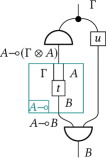
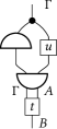
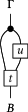
(a) Proving (BR) using functoriality of $-\otimes A$, naturality of eval, and adjunction cancellation

= =

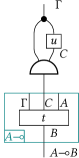
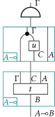
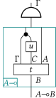
(b) Proving (Lamb) using naturality of coeval and functoriality of $A\multimap-$

Figure 5. Axioms of the $\Lambda$es and their proofs.

Finally, the CE structural rule is also rather interesting, as it requires proving that  = . The proof is an immediate consequence of the functoriality of the tensor and of the identity law. What is interesting is that the two diagrams look very similar as graphs. Indeed, the intuition that diagrams represented by isomorphic graphs denote equal morphisms will be made rigorous in Sec. LABEL:sec:hypernet.

To emphasise the syntactic nature of the transformation we will call the objects the types of the diagrams. Since we are situated in a strict-monoidal setting we will write a composite tensor of objects as a list of types. We write a generic typed term $t:A_{1}\otimes\cdots\otimes A_{m}\multimap A_{1}^{\prime}\otimes\cdots\otimes A_{n}^{\prime}$ in the language of string diagrams as $:\left(\stackanchor{$[A_{1},\ldots,A_{m}]$}{$[A_{1}^{\prime},\ldots,A_{n}^{\prime}]$}\right)$.

3. A graphical AD algorithm

This section represents the main technical result of our paper, to define and and prove the soundness of an algorithm for performing reverse-mode automatic differentiation on hierarchical string diagrams. The algorithm can be considered a simplified version of that presented in (DBLP:journals/toplas/PearlmutterS08). This algorithm is remarkable for being one of the first such algorithms that can be applied to code containing closures and higher-order functions. It is particularly in the treatment of higher-order features where we draw inspiration from their work.

The soundness property of the algorithm is technically interesting because simple inductive proofs of correctness do not seem possible. If simply taking the gradient of a higher-order function, the algorithm is actually unsound. However, when taking the gradient of a function with ground-type inputs and outputs only, the results are correct even if the function contains higher-order terms.

Unlike the original algorithm, however, we do not provide automatic differentiation as a first-class entity. This means, implicitly, that we also do not have a means to perform ‘higher order differentiation’ in the sense of differentiating the differential operator itself. In the original work, this was achieved by extending the language with rich runtime reflection capabilities whose formalisation is entirely outside of the scope of our paper. Our algorithm instead is formulated as a meta-level set of rules on hierarchical string diagrams or, in actual implementation, on their hypernet representation. This is akin to the source-to-source transformation approach to automatic differentiation.

The setting for this algorithm is that of a (strict) cartesian closed category generated from one object $o::=\mathcal{R}$, representing the real numbers, and a collection of primitive operations (addition, multiplication, trigonometric functions, etc.) and their gradients, along with a collection of nullary primitive operations for real constants. Among these, real addition and zero must be included. In the string diagrams throughout this section we represent constants as a triangle instead of a box, just for improved readability. We write and for the obvious extension of and to bundles.

Each of the provided primitive operations must also come equipped with a pullback diagram: for a primitive operation of type $\left(\stackanchor{$B$}{$B^{\prime}$}\right)$, its pullback diagram must have type $\left(\stackanchor{$B::B^{\prime}$}{$B$}\right)$. We make no assumptions about the pullback diagram of an operator, other than its type. However, the correctness result in this section will require pullback diagrams to be ‘correct’ implementations of the gradient of the corresponding operation.

3.1. Rewrite rules on string diagrams

The AD algorithm consists of three separate sets of transformations, the application of which we denote by differently coloured boxes around a diagram. We emphasise that these boxes represent meta-level transformations, and are not to be confused with object-level entities such as the rounded rectangles that we use to denote abstraction.

To reduce clutter we use coloured boxes rather than labelled frames to indicate string-diagram transformations. The first transformation, whose only rewrite rule can be found in Fig. 6, is denoted by a blue box and is the entry point of the algorithm. Given an input diagram with operands of type $B$ and results of type $B^{\prime}$, this transformation produces an adjoint diagram with operands of type $B$ and results of type $B::[B^{\prime}\multimap B]$, corresponding to the result of the original diagram plus an abstraction, the backpropagator, that computes the gradient of the original diagram at the point at which the adjoint diagram is evaluated. In particular, if the original diagram produces a single result of type $\mathcal{R}$, when evaluating the backpropagator at $1.0$ we will obtain the gradient of the original diagram.

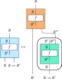
Figure 6. Adjoint rule

This transformation consists, in turn, of two components: a forward pass transformation (in orange), rewrite rules in Fig. 7(a)) and a reverse pass transformation (in green), rewrite rules in Fig. 7(b)). As the naming suggests, these correspond to the forward and reverse passes commonly employed in reverse-mode AD. The forward pass executes the original function ‘as is’, whereas the reverse pass computes the gradient of every sub-expression, in reverse order of execution. In our algorithm, as is usually the case in reverse-mode AD systems, some intermediate values computed during the forward pass are preserved and passed along to the diagram corresponding to the reverse pass. This is shown in Fig. 6 as a bundle of type $B^{\prime\prime}$ flowing from the forward-pass computation into the backpropagator.

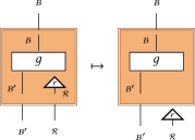
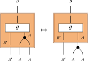
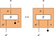
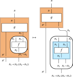
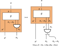
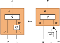
(a) Rewrites defining the forward pass

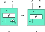
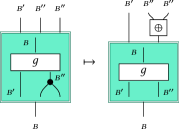
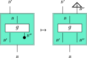
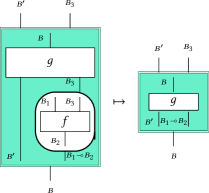
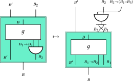
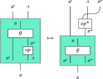
(b) Rewrites defining the reverse pass

Figure 7. Forward and reverse pass rewrites

The rewrites for the forward-pass transformation, depicted in Fig. 7(a), are self-explanatory, as they are limited to constructing a copy of the original diagram. Only two cases (those for evaluation and abstraction) merit some attention. For abstraction, the diagram enclosed by the bubble is recursively transformed using the blue rule — that is, any abstraction in the primal diagram is replaced by a new abstraction that computes the adjoint of the original one. Then, when function evaluation in the primal diagram is translated by the forward pass, the result of the adjoint application contains both the result of the original abstraction and a backpropagator which is not used in the forward pass but is set aside for the reverse pass.

Figure 8. Pullback diagrams for some common operations

The rules governing the reverse pass transformation, in Fig. 7(b), are more involved, so we provide here an intuitive explanation for each. The first rule, which handles constants, states that constants do not contribute to the gradient of the graph. The second rule computes the gradient of the identity function to be the identity. Contraction is transformed into addition, since the gradient of the diagonal map $\langle\text{id},\text{id}\rangle$ is the addition of tangent vectors, and weakened variables become zero. Each primitive operation is replaced by its corresponding pullback diagram, which receives as additional operands the copies of the inputs to the operation in the forward pass. This is why we require that every primitive operation to be mapped to a pullback diagram of the appropriate type. Some examples of pullback diagrams for common operations can be found in Fig. 8.

The reverse pass handling of application and abstraction are, both in the original algorithm and in our interpretation of it, difficult to back up with compelling intuitions, but we shall try our best.

Remember that the forward pass transforms every abstraction in the primal diagram in order to compute the original value together with a backpropagator. The latter is captured by the reverse pass in every application rule. When rewriting an application node, the reverse pass instead applies the backpropagator given by the forward rule. This backpropagator in turn produces a wire for every operand of the body of the original abstraction, which are swapped into the correct order. The abstraction rule in the reverse pass then expects the sensitivity of an abstraction to consist of a bundle of wires corresponding to the sensitivities of each captured wire.

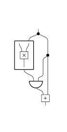
(a) Primal diagram

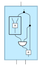
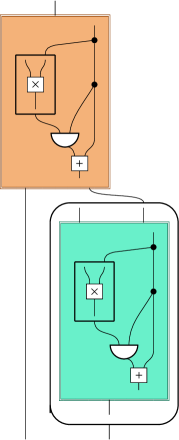
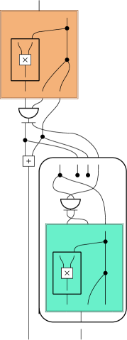
$\mapsto$ $\mapsto$ $\mapsto$

(b)

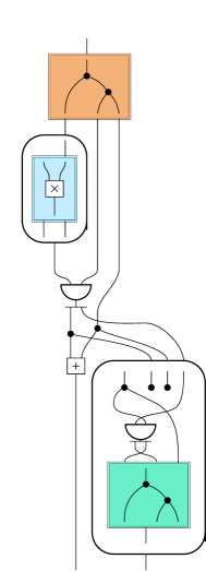
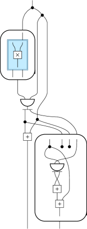
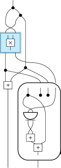
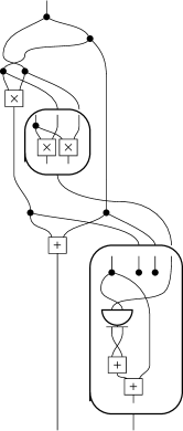
$\mapsto$ $\mapsto$ $\mapsto$ $\mapsto$

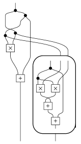
(b) Adjoint diagram

Figure 9. The AD transformation on a string diagram diagram computing $x^{2}+x$

As an example illustrating this algorithm and its handling of closures in particular, we provide in Fig. 9(a) a diagram that might result from a program like let mul y = x * y in mul x + x, with the free variable x corresponding to its single operand. On the right, in Fig. 9(b), we show the result of applying the adjoint transformation to this diagram (see Appendix LABEL:appendix:animations for an animated step-by-step derivation). It is a mere calculation to check that the resulting backpropagator, when applied to input $1$, can be evaluated to the correct derivative of the polynomial $x^{2}+x$.

Lemma 3.1.

The rewriting systems in Fig. 7(a) and Fig. 7(b) have the diamond property, up to a permutation of the output wires.

Proof (Sketch).

Every rule erases one node in the fringe of the left-hand side diagram, and that no two rules can be applied to erase the same node. Therefore, if two rules can apply to the same diagram, it must be the case that they apply to different fringe nodes. It is then easily checked that every pair of such rules commutes, modulo a permutation of the wires that are propagated from the forward to the reverse pass. For a concrete example, consider the two sequences of rewrites in Fig. LABEL:fig:diamond. ∎

$\mapsto$

$\mapsto$

$\mapsto$      

$\mapsto$