The role of right-handed neutrinos in $b\to c\tau\,(\pi\nu_{\tau},\rho\nu_{\tau},\mu\bar{\nu}_{\mu}\nu_{\tau})\bar{\nu}_{\tau}$ from visible final-state kinematics

Abstract

In the context of lepton flavor universality violation (LFUV) studies, we fully derive a general tensor formalism to investigate the role that left- and right-handed neutrino new-physics (NP) terms may have in $b\to c\tau\bar{\nu}_{\tau}$ transitions. We present, for several extensions of the Standard Model (SM), numerical results for the $\Lambda_{b}\to\Lambda_{c}\tau\bar{\nu}_{\tau}$ semileptonic decay, which is expected to be measured with precision at the LHCb. This reaction can be a new source of experimental information that can help to confirm, or maybe rule out, LFUV presently seen in $\bar{B}$ meson decays. The present study analyzes observables that can help in distinguishing between different NP scenarios that otherwise provide very similar results for the branching ratios, which are our currently best hints for LFUV. Since the $\tau$ lepton is very short-lived, we consider three subsequent $\tau$-decay modes, two hadronic $\pi\nu_{\tau}$ and $\rho\nu_{\tau}$ and one leptonic $\mu\bar{\nu}_{\mu}\nu_{\tau}$, which have been previously studied for $\bar{B}\to D^{(*)}$ decays. Within the tensor formalism that we have developed in previous works, we re-obtain the expressions for the differential decay width written in terms of visible (experimentally accessible) variables of the massive particle created in the $\tau$ decay. There are seven different $\tau$ angular and spin asymmetries that are defined in this way and that can be extracted from experiment. Those asymmetries provide observables that can help in constraining possible SM extensions.

1 Introduction

Although there is no single experiment that can still claim the discovery of new physics (NP) beyond the Standard Model (SM), there seems to be however mounting evidence that points in that direction. Lepton flavor universality (LFU), which is inherent to the SM (the exception made of lepton-Higgs couplings), is being challenged in different experiments. Thus, the ${\cal R}_{D^{(*)}}=\frac{\Gamma(\bar{B}\to D^{(*)}\tau\bar{\nu}_{\tau})}{\Gamma(\bar{B}\to D^{(*)}\ell\bar{\nu}_{\ell})}$ ratios, with $\ell=e,\mu$, show a $3.1\sigma$ tension Amhis:2019ckw with SM results and the similar ${\cal R}_{J/\psi}=\frac{\Gamma(\bar{B}_{c}\to J/\psi\tau\bar{\nu}_{\tau})}{\Gamma(\bar{B}_{c}\to J/\psi\mu\bar{\nu}_{\mu})}$ observable, recently measured by the LHCb Collaboration Aaij:2017tyk , provides also a $1.8\,\sigma$ discrepancy with different SM evaluations Anisimov:1998uk ; Ivanov:2006ni ; Hernandez:2006gt ; Huang:2007kb ; Wang:2008xt ; Wen-Fei:2013uea ; Watanabe:2017mip ; Issadykov:2018myx ; Tran:2018kuv ; Hu:2018veh ; Wang:2018duy ; Hu:2019qcn ; Leljak:2019eyw ; Azizi:2019aaf .

In the absence of a unique possible extension of the SM, one tries to explain the discrepancies adopting a phenomenological strategy including, besides NP corrections to the SM vector and axial terms, NP scalar, pseudoscalar and tensor $b\to c\tau\bar{\nu}_{\tau}$ effective operators that, in principle, affect only the third quark and lepton generations. Typically, only left-handed neutrinos are considered. The strength of the different NP operators is governed by, complex in general, Wilson coefficients that encode the NP low energy effects and that are fitted to data.

Further experimental information may come from the analysis of the $\Lambda_{b}\to\Lambda_{c}$ semileptonic decays. In fact, the shape of the $d\Gamma(\Lambda_{b}\to\Lambda_{c}\mu^{-}\bar{\nu}_{\mu})/d\omega$ decay width has already been measured by the LHCb Collaboration Aaij:2017svr , and there are expectations Cerri:2018ypt that the ${\cal R}_{\Lambda_{c}}=\frac{\Gamma(\Lambda_{b}\to\Lambda_{c}\tau\bar{\nu}_{\tau})}{\Gamma(\Lambda_{b}\to\Lambda_{c}\mu\bar{\nu}_{\mu})}$ ratio can be obtained with a similar precision to that reached for ${\cal R}_{D^{(*)}}$. From the theoretical point of view, there are precise Lattice QCD determinations of the vector and axial form factors Detmold:2015aaa , as well as the NP tensor ones Datta:2017aue . The scalar and pseudoscalar form factors, also needed for a full description of all NP terms on the low energy Hamiltonian comprising the full set of dimension-6 operators, can be directly related to vector and axial ones (see Eqs. (2.12) and (2.13) of Ref. Datta:2017aue ). This allows for a reliable SM determination of ${\cal R}_{\Lambda_{c}}$  Gutsche:2015mxa ; Azizi:2018axf ; Bernlochner:2018kxh , as well as the evaluation of NP effects Dutta:2015ueb ; Shivashankara:2015cta ; Ray:2018hrx ; Li:2016pdv ; Datta:2017aue ; Blanke:2018yud ; Bernlochner:2018bfn ; DiSalvo:2018ngq ; Blanke:2019qrx ; Boer:2019zmp ; Murgui:2019czp ; Ferrillo:2019owd ; Mu:2019bin ; Colangelo:2020vhu ; Hu:2020axt that can be compared to future experimental determinations.

Although the latest measurements of the ${\cal R}_{D^{(*)}}$ ratios by the Belle Collaboration Belle:2019rba constraint the admissible extensions of the SM Shi:2019gxi , disfavoring for instance large pure tensor NP scenarios, there is not a unique NP solution to solve the discrepancies (see Refs. Bhattacharya:2018kig ; Murgui:2019czp ; Shi:2019gxi ) and, thus, other observables have been proposed as benchmarks to constrain and/or determine the most favored NP extension of the SM. These include asymmetries, like the $\tau$-forward-backward (${\cal A}_{FB}$) and $\tau$-polarization (${\cal A}_{\lambda_{\tau}}$) ones, but also different observables related to the four-body $\bar{B}\to D^{*}(D\pi,D\gamma)\tau\bar{\nu}_{\tau}$  Duraisamy:2013pia ; Duraisamy:2014sna ; Becirevic:2016hea ; Colangelo:2018cnj and the full five-body $\bar{B}\to D^{*}(DY)\tau(X\nu_{\tau})\bar{\nu}_{\tau}$ Ligeti:2016npd ; Bhattacharya:2020lfm angular distributions.

The transverse components of the $\tau$ polarization vector ${\cal P}^{\mu}$ are also different sources of information. For instance, the $\tau$ polarization vector component perpendicular to the plane defined by the $\tau$ and final hadron three-momenta, $P_{TT}$, is nonzero only for complex Wilson coefficients. Its measurement will not only be an indication of NP beyond the SM but also of CP violation. The search for NP in different $\tau$-polarization observables for $\bar{B}\to D^{(*)}$ decays was explored already twenty five years ago in the context of SM extensions with charged Higgs bosons Tanaka:1994ay . More recent works Nierste:2008qe ; Tanaka:2012nw ; Ivanov:2017mrj ; Alonso:2016gym ; Alonso:2017ktd ; Blanke:2018yud ; Asadi:2020fdo have developed this idea. In Ref. Penalva:2021gef , within the formalism previously developed in Refs. Penalva:2019rgt ; Penalva:2020xup , we have evaluated the different components of the tau polarization vector (${\cal P}^{\mu}$) for the $\Lambda_{b}\to\Lambda_{c}$, $\bar{B}_{c}\to\eta_{c},J/\psi$ and $\bar{B}\to D^{(*)}$ semileptonic decays, for extensions of the SM involving only left-handed neutrino operators. We have described NP effects in the complete two-dimensional space, corresponding to the two independent kinematical variables on which ${\cal P}^{\mu}$ depends, finding that its detailed study has indeed a great potential to discriminate between different NP scenarios for $0^{-}\to 0^{-}$ decays and also for the $\Lambda_{b}\to\Lambda_{c}$ transition.

A caveat in some of the above $\tau$ polarization-vector analyses is that to experimentally measure some of the observables one needs to be able to establish the $\tau$ three-momenta. This is however extremely difficult due to the $\tau$ lepton being very short-lived and the fact that the decay products contain neutrinos which escape detection. A way out of this problem is to concentrate on what is termed as visible kinematics. This is achieved by considering the subsequent $\tau$ decay and integrating out all variables that can not be directly measured, either neutrino-related ones or variables defined with respect to the $\tau$ three-momentum. The price to pay is that one can only access averages of the full polarization vector components and that all the information on $P_{TT}$ is lost after the integration process. This is for instance what was done, for the $\bar{B}\to D^{(*)}$ reaction in Ref. Alonso:2017ktd , where, the authors concentrated in the two subsequent $\tau\to\pi\nu_{\tau}$ and $\tau\to\rho\nu_{\tau}$ hadronic decay modes. Further, in Ref. Asadi:2020fdo , it was shown how to extract a total of seven $\tau$ angular and spin asymmetries from a full analysis of the final-state visible kinematics. A similar study, also for the $\bar{B}\to D^{(*)}$ reaction but considering in this case the purely leptonic $\tau\to\mu\bar{\nu}_{\mu}\nu_{\tau}$ decay mode, was carried out in Ref. Alonso:2016gym .

In this work we shall present an analysis parallel to what was done in Refs. Alonso:2016gym ; Alonso:2017ktd ; Asadi:2020fdo , but centered in this case in the $\Lambda_{b}\to\Lambda_{c}\tau\bar{\nu}_{\tau}$ semileptonic decay. We only know of one analysis of this reaction in terms of visible kinematical variables done in Ref. Hu:2020axt . There, the authors construct a measurable angular distribution for the full five body decay $\Lambda_{b}\to\Lambda_{c}(\Lambda\pi)\tau(\pi\nu_{\tau})\bar{\nu}_{\tau}$ in terms of ten angular observables and they provide results within the SM and different NP models with left-handed neutrinos. Three of these observables can be written as linear combinations of the three $F_{0,1,2}^{\pi}$ functions that we introduce in Eq. (69). Note however that, following Refs. Alonso:2016gym ; Alonso:2017ktd ; Asadi:2020fdo , we decompose the latter functions in a total of seven angular and spin asymmetries (see Eq. (70) for the pion $\tau$-decay mode) that, together with the overall normalization, can give separate information on NP and that, hence, we analyze separately. The rest of the angular observables analyzed in Ref. Hu:2020axt can not be accessed in our work since they require to consider the further $\Lambda_{c}\to\Lambda\pi$ decay. In our case we shall also focus on NP extensions that include right-handed neutrino terms. The latter have been suggested Greljo:2018ogz ; Asadi:2018wea ; Robinson:2018gza ; Azatov:2018kzb ; Mandal:2020htr as a way to evade present constraints on NP effective operators with only left-handed neutrinos. Since interference with the dominant SM left-handed terms cancels for massless neutrinos, the contributions from right-handed operators are quadratic in the corresponding Wilson coefficients. This means that larger values of the Wilson coefficients may be needed for a purely right-handed NP explanation of the discrepancies between SM results and experimental data, which has to be balanced with the fact that large values of the corresponding right-handed NP Wilson coefficients are more in tension with other low-energy observables or collider searches Alonso:2016oyd ; Akeroyd:2017mhr ; Greljo:2018tzh . Here we shall use three different models that include right-handed neutrino NP terms and that we take from Ref. Mandal:2020htr . The results obtained within those fits will be compared, not only with SM results, but also with the ones obtained from Fit 7 of Ref. Murgui:2019czp , which contains pure left-handed neutrino NP operators.

The calculations will be done within the tensor formalism that we developed in Refs. Penalva:2019rgt ; Penalva:2020xup for left-handed neutrino NP operators, which is extended in the present work to account also for NP terms constructed out of light right-handed neutrino fields. It is based on the use of hadron tensors and it provides a general description of any semileptonic decay process where all hadron polarizations are summed/averaged, being in those cases a useful alternative to the commonly used helicity amplitude approach. Within the tensor formalism, we have previously analyzed the $\tau$ polarization vector Penalva:2021gef , but also the role that different contributions to the differential decay widths $d^{2}\Gamma/(d\omega d\cos\theta_{\tau})$ and $d^{2}\Gamma/(d\omega dE_{\tau})$, both in the unpolarized and tau helicity-polarized cases, could play in the search of NP Penalva:2019rgt ; Penalva:2020xup ; Penalva:2020ftd . In the above, $\omega$ stands for the product of the initial and final hadron four-velocities, $\theta_{\tau}$ is the angle made by the three-momenta of the tau and final hadron in the center of mass of the final two-lepton pair (CM), and $E_{\tau}$ is the energy of the tau lepton in the frame where the initial hadron is at rest (LAB). Our studies showed that the helicity-polarized distributions in the LAB frame provide information on NP contributions that cannot be accessed from the study of the CM differential decay width, the one that is commonly analyzed in the literature. Besides, we have found that $0^{-}\to 0^{-}$ and $1/2^{+}\to 1/2^{+}$ decays seem to better discriminate between different left-handed neutrino NP than $0^{-}\to 1^{-}$ reactions.

The present work is organized as follows: In section 2, together with appendices A, B, C and D, we review our tensor formalism, and extend it to include right-handed neutrino NP terms. We want to stress here that although we always refer to $b\to c$ transitions, the hadron and lepton tensors, together with the expressions for the semileptonic differential distributions derived in this work, in the presence of both left- and right-handed neutrino NP terms, are valid for any $q\to q^{\prime}\ell\bar{\nu}_{\ell}$ charged-current decay. In section 2.3 we collect some of the main theoretical expressions obtained in Ref. Penalva:2021gef concerning the spin density operator and the $\tau$ polarization vector, which will be needed in the next section. Besides, an extension of these results to the case of a $\bar{b}\to\bar{c}$ transition is presented (see also appendix E in this latter respect). In section 3, we make a thorough study of the $H_{b}\to H_{c}\tau\bar{\nu}_{\tau}$ reaction including the subsequent $\tau$-decay, for which we shall consider the two hadronic decay modes $\tau\to\pi\nu_{\tau}$ and $\tau\to\rho\nu_{\tau}$ and the leptonic one $\tau\to\mu\bar{\nu}_{\mu}\nu_{\tau}$. Although we also provide differential decay widths with respect to variables defined in the $\tau$ rest frame, we mainly concentrate in obtaining the differential decay width in terms of visible kinematic variables and we identify (section 3.4) the seven $\tau$ angular and spin asymmetries mentioned above. Some details on the evaluation of the phase-space integrals, which can be rather involved in the leptonic decay mode, are presented in appendix F, while the kinematical coefficients that multiply each of the observables are discussed in appendix G. Results for the $\tau$ asymmetries in the $\Lambda_{b}\to\Lambda_{c}$ transition are presented in section 4. They are obtained within the SM, three different NP extensions that include right-handed neutrino fields, and a NP model constructed with left-handed neutrino operators alone. A short summary of our main findings is given in section 5.

2 Hadron and lepton tensors in semileptonic decays including new physics with right-handed neutrinos

In Refs. Penalva:2019rgt ; Penalva:2020xup , we derived a general framework, based on the use of general hadron tensors parameterized in terms of Lorentz scalar functions, for describing any meson or baryon semileptonic decay. It is an alternative to the helicity-amplitude scheme for the description of processes where all hadron polarizations are summed up and/or averaged. In these two works, NP with left-handed neutrinos were considered, and here we extend the formalism to include also right-handed neutrino operators.

2.1 Effective Hamiltonian

We consider an extension of the SM based on the low-energy Hamiltonian comprising the full set of dimension-6 semileptonic $b\to c$ operators with left- and right-handed neutrinos Mandal:2020htr

$$H_{\rm eff} = \frac{4G_{F}V_{cb}}{\sqrt{2}}\left[(1+C^{V}_{LL}){\cal O}^{V}_{LL}+C^{V}_{RL}{\cal O}^{V}_{RL}+C^{S}_{LL}{\cal O}^{S}_{LL}+C^{S}_{RL}{\cal O}^{S}_{RL}+C^{T}_{LL}{\cal O}^{T}_{LL}\right.$$ (1)

$$+ \left.C^{V}_{LR}{\cal O}^{V}_{LR}+C^{V}_{RR}{\cal O}^{V}_{RR}+C^{S}_{LR}{\cal O}^{S}_{LR}+C^{S}_{RR}{\cal O}^{S}_{RR}+C^{T}_{RR}{\cal O}^{T}_{RR}\right]+h.c.,$$

with left-handed neutrino fermionic operators given by

$${\cal O}^{V}_{(L,R)L}=(\bar{c}\gamma^{\mu}b_{L,R})(\bar{\ell}\gamma_{\mu}\nu_{\ell L}),\,{\cal O}^{S}_{(L,R)L}=(\bar{c}\,b_{L,R})(\bar{\ell}\,\nu_{\ell L}),\,{\cal O}^{T}_{LL}=(\bar{c}\,\sigma^{\mu\nu}b_{L})(\bar{\ell}\sigma_{\mu\nu}\nu_{\ell L})$$ (2)

and the right-handed neutrino ones

$${\cal O}^{V}_{(L,R)R}=(\bar{c}\gamma^{\mu}b_{L,R})(\bar{\ell}\gamma_{\mu}\nu_{\ell R}),\,{\cal O}^{S}_{(L,R)R}=(\bar{c}\,b_{L,R})(\bar{\ell}\,\nu_{\ell R}),\,{\cal O}^{T}_{RR}=(\bar{c}\,\sigma^{\mu\nu}b_{R})(\bar{\ell}\sigma_{\mu\nu}\nu_{\ell R}),$$ (3)

and where $\psi_{R,L}=(1\pm\gamma_{5})\psi/2$, $G_{F}=1.166\times 10^{-5}$ GeV^-2 and $V_{cb}$ is the corresponding Cabibbo-Kobayashi-Maskawa matrix element. Note that tensor operators with different lepton and quark chiralities vanish identically.

The 10 Wilson coefficients $C^{X}_{AB}$ ($X=S,V,T$ and $A,B=L,R$) parametrize possible deviations from the SM, i.e. $C^{X}_{AB}\big{|}_{\rm SM}$=0. They are lepton and flavour dependent, and complex in general.

2.2 Hadron and lepton currents

The semileptonic differential decay rate of a bottomed hadron ($H_{b}$) of mass $M$ into a charmed one ($H_{c}$) of mass $M^{\prime}$ and $\ell\bar{\nu}_{\ell}$, measured in its rest frame, after averaging (summing) over the initial (final) hadron polarizations, reads Tanabashi:2018oca ,

$$\frac{d^{2}\Gamma}{d\omega ds_{13}}=\Gamma_{0}\,\overline{\sum}\ |{\cal M}|^{2},\qquad\Gamma_{0}=\frac{G^{2}_{F}|V_{cb}|^{2}M^{\prime 2}}{(2\pi)^{3}M},$$ (5)

where ${\cal M}(k,k^{\prime},p,q,\,{\rm spins})$ is the transition matrix element, with $p$, $k^{\prime}$, $k=q-k^{\prime}$ and $p^{\prime}=p-q$, the decaying $H_{b}$ particle, outgoing charged-lepton, neutrino and final hadron four-momenta, respectively. In addition, $\omega$ is the product of the two hadron four velocities $\omega=(p\cdot p^{\prime})/(MM^{\prime})$, which is related to $q^{2}=(k+k^{\prime})^{2}$ via $q^{2}=M^{2}+M^{\prime 2}-2MM^{\prime}\omega$, and $s_{13}=(p-k)^{2}$. Including both left- and right-handed neutrino NP contributions, we have

$${\cal M}=\left(J_{H}^{\alpha}J^{L}_{\alpha}+J_{H}J^{L}+J_{H}^{\alpha\beta}J^{L}_{\alpha\beta}\right)_{\nu_{\ell L}}+\left(J_{H}^{\alpha}J^{L}_{\alpha}+J_{H}J^{L}+J_{H}^{\alpha\beta}J^{L}_{\alpha\beta}\right)_{\nu_{\ell R}},\\$$ (7)

with the polarized lepton currents given by ($u$ and $v$ dimensionful Dirac spinors)

$$J^{L}_{(\alpha\beta)}(k,k^{\prime};h,h_{\chi}) = \frac{1}{\sqrt{2}}\bar{u}_{\ell}^{S}(k^{\prime};h)\Gamma_{(\alpha\beta)}P_{5}^{h_{\chi}}v_{\bar{\nu}_{\ell}}(k),$$

$$\Gamma_{(\alpha\beta)} = 1,\gamma_{\alpha},\sigma_{\alpha\beta},\quad P_{5}^{h_{\chi}}=\frac{1+h_{\chi}\gamma_{5}}{2},$$ (8)

where $h=\pm 1$ stand for the two possible charged-lepton polarizations (covariant spin) along a certain four vector $S^{\alpha}$ that we choose to measure in the experiment. This is to say, the outgoing charged-lepton is produced in the state $u^{S}_{\ell}(k^{\prime};h)$ defined by the condition

$$\gamma_{5}\not{S}\,u^{S}_{\ell}(k^{\prime};h)=h\,u^{S}_{\ell}(k^{\prime};h).$$ (9)

The four vector $S^{\alpha}$ satisfies the constraints $S^{\,2}=-1$ and $S\cdot k^{\prime}=0$, and the choice $S^{\alpha}=(|\vec{k}^{\prime}|,k^{\prime 0}\hat{k}^{\prime})/m_{\ell}$, with $\hat{k}^{\prime}=\vec{k}^{\prime}/|\vec{k}^{\prime}|$ and $m_{\ell}$ the charged lepton mass, leads to charged-lepton helicity states. For later purposes we define here the projector

$$P_{h}=\frac{1+h\gamma_{5}\not{S}}{2}.$$ (10)

In addition, $h_{\chi}$ accounts for both neutrino chiralities, $R(h_{\chi}=1)$ and $L(h_{\chi}=-1)$.

The dimensionless hadron currents read

$$J_{Hrr^{\prime}\,\chi(=L,R)}^{(\alpha\beta)}(p,p^{\prime})=\langle H_{c};p^{\prime},r^{\prime}|\bar{c}(0)O_{H\chi}^{(\alpha\beta)}b(0)|H_{b};p,r\rangle,$$ (11)

with $c(x)$ and $b(x)$ Dirac fields in coordinate space, hadron states normalized as $\langle\vec{p}\,^{\prime},r^{\prime}|\vec{p},r\rangle=(2\pi)^{3}(E/M)\delta^{3}(\vec{p}-\vec{p}\,^{\prime})\delta_{rr^{\prime}}$ with $r,r^{\prime}$ spin indexes, and (we recall $h_{\chi=R}=+1$ and $h_{\chi=L}=-1$)

$$O_{H\chi}^{(\alpha\beta)}=(C^{S}_{\chi}+h_{\chi}C^{P}_{\chi}\gamma_{5}),\qquad(C^{V}_{\chi}\gamma^{\alpha}+h_{\chi}C^{A}_{\chi}\gamma^{\alpha}\gamma_{5}),\qquad C^{T}_{\chi}\sigma_{\alpha\beta}(1+h_{\chi}\gamma_{5}).$$ (12)

The Wilson coefficients $C_{\chi=L,R}^{S,P,V,A,T}$ in the above definitions are linear combinations of those introduced in the effective Hamiltonian of Eq. (1) and are given in Appendix A. Neglecting the neutrino mass, $m_{\nu_{\ell}}$, there is no interference between the two neutrino chiralities, and the decay probability becomes an incoherent sum of $\nu_{\ell L}$ and $\nu_{\ell R}$ contributions,

$$|{\cal M}|^{2}=|{\cal M}|_{\nu_{\ell L}}^{2}+|{\cal M}|_{\nu_{\ell R}}^{2}+{\cal O}(m_{\nu_{\ell}}/E_{\nu_{\ell}}),$$ (13)

with $E_{\nu_{\ell}}$ the neutrino energy. The diagonal lepton tensors needed to obtain $|{\cal M}|^{2}$ are readily evaluated and they are collected in Appendix B for $m_{\nu_{\ell}}=0$.

After summing over polarizations, the hadron contributions can be expressed in terms of Lorentz scalar structure functions (SFs), which depend on $q^{2}$, the hadron masses and the 10 NP Wilson coefficients, $C^{X}_{AB}$, introduced in the effective Hamiltonian of Eq.(1). Lorentz, parity and time-reversal transformations of the hadron currents (Eq. (12)) and states Itzykson:1980rh limit their number, as discussed in detail in Ref. Penalva:2020xup . The hadron tensors are expressed as linear combination of independent Lorentz (pseudo-)tensor structures, constructed out of the vectors $p^{\mu}$, $q^{\mu}$, the metric $g^{\mu\nu}$ and the Levi-Civita pseudotensor $\epsilon^{\mu\nu\delta\eta}$. The coefficients multiplying the (pseudo-)tensors are the $\widetilde{W}^{{}^{\prime}s}_{\chi=L,R}$ SFs. They depend on $q^{2}$, the hadron masses, the Wilson coefficients for each neutrino chirality ($C^{V,A,S,P,T}_{\chi=L,R}$), and the genuine hadronic responses ($W^{\prime}s$). The latter ones are determined by the matrix elements of the involved hadron operators, which for each particular decay are parametrized in terms of form-factors. Symbolically, we have $\widetilde{W}_{\chi}=C_{\chi}W$. There is a total of 16 independent SFs ($\widetilde{W}^{{}^{\prime}s}_{\chi}$) for each neutrino-chirality set of Wilson coefficients, as shown in Ref. Penalva:2020xup . However, the consideration of both neutrino chiralities does not modify the number of genuine hadronic responses $W^{\prime}s$, and the number of $\widetilde{W}$ SFs increases due to the greater number of Wilson coefficients. For the sake of clarity, the definition of the $\widetilde{W}^{{}^{\prime}s}_{\chi}$ SFs are compiled here in Appendix C.

From the general structure of the lepton and hadron tensors, collected in Appendices B and C, and which are at most quadratic in $k,k^{\prime}$ and $p$, one can generally write for the decay with a polarized charged lepton. Penalva:2020xup ; Penalva:2021gef

$$\frac{2\,\overline{\sum}\,|{\cal M}|^{2}}{M^{2}} \simeq \frac{2\,\overline{\sum}\,\left(|{\cal M}|_{\nu_{\ell L}}^{2}+|{\cal M}|_{\nu_{\ell R}}^{2}\right)}{M^{2}}={\cal N}(\omega,p\cdot k)+h\bigg{\{}\frac{(p\cdot S)}{M}\,{\cal N_{H_{\rm 1}}}(\omega,p\cdot k)$$ (14)

$$+ \frac{(q\cdot S)}{M}\,{\cal N_{H_{\rm 2}}}(\omega,p\cdot k)+\frac{\epsilon^{Sk^{\prime}qp}}{M^{3}}\,{\cal N_{H_{\rm 3}}}(\omega,p\cdot k)\ \bigg{\}},$$

with $\epsilon^{Sk^{\prime}qp}=\epsilon^{\alpha\beta\rho\lambda}S_{\alpha}k^{\prime}_{\beta}q_{\rho}p_{\lambda}$ and the ${\cal N}$ and $\cal N_{H_{\rm 123}}$ scalar functions given by

$${\cal N}(\omega,k\cdot p) = \frac{1}{2}\Big{[}{\cal A}(\omega)+{\cal B}(\omega)\frac{(k\cdot p)}{M^{2}}+{\cal C}(\omega)\frac{(k\cdot p)^{2}}{M^{4}}\Big{]},$$

$${\cal N_{H_{\rm 1}}}(\omega,k\cdot p) = {\cal A_{H}}(\omega)+{\cal C_{H}}(\omega)\frac{(k\cdot p)}{M^{2}},$$

$${\cal N_{H_{\rm 2}}}(\omega,k\cdot p) = {\cal B_{H}}(\omega)+{\cal D_{H}}(\omega)\frac{(k\cdot p)}{M^{2}}+{\cal E_{H}}(\omega)\frac{(k\cdot p)^{2}}{M^{4}},$$

$${\cal N_{H_{\rm 3}}}(\omega,k\cdot p) = {\cal F_{H}}(\omega)+{\cal G_{H}}(\omega)\frac{(k\cdot p)}{M^{2}}.$$ (15)

There are three independent functions, ${\cal A},{\cal B}$, and ${\cal C}$ , for the non-polarized case, and seven additional ones, ${\cal A_{H}},{\cal B_{H}},{\cal C_{H}},{\cal D_{H}}$, ${\cal E_{H}}$, ${\cal F_{H}}$ and ${\cal G_{H}}$, to describe the process with a defined polarization ($h=\pm 1$) of the outgoing $\ell$ along the four vector $S^{\alpha}$. Expressions for all of them in terms of the $\widetilde{W}$ SFs are given in Appendix D. As can be seen there, these functions receive contributions from both neutrino chiralities. For ${\cal A},{\cal B}$, ${\cal C}$, ${\cal F_{H}}$ and ${\cal G_{H}}$, it always appears the combination $(L+R)$, i.e. $(\widetilde{W}_{iL}+\widetilde{W}_{iR})$, while for the other functions (${\cal A_{H}},{\cal B_{H}},{\cal C_{H}},{\cal D_{H}}$ and ${\cal E_{H}}$) the structure is ($L-R):$ ($\widetilde{W}_{iL}-\widetilde{W}_{iR})$. An obvious consequence is that the NP $L-$ and $R-$neutrino-chirality contributions cannot be disentangled using only the non-polarized decay, and some information is needed from charged-lepton polarized distributions.

As can be seen in Appendices C and D, the $\widetilde{W}$ SFs present in ${\cal N_{H_{\rm 3}}}$ are generated from the interference of vector-axial with scalar-pseudoscalar terms ($\widetilde{W}_{I1\chi}$), scalar-pseudoscalar with tensor terms ($\widetilde{W}_{I3\chi}$), and vector-axial with tensor terms ($\widetilde{W}_{I4\chi,I5\chi,I6\chi}$). Since the vector-axial terms are already present in the SM, at least one of the $C^{S,P,T}_{\chi}$ coefficients must be non-zero to generate a non-zero ${\cal N_{H_{\rm 3}}}$ term. Besides, ${\cal N_{H_{\rm 3}}}$ is proportional to the imaginary part of SFs, which requires complex Wilson coefficients, thus incorporating violation of the CP symmetry in the NP effective Hamiltonian. This feature makes the study of such contribution of special relevance.

As expected, the ${\cal N}(\omega,k\cdot p)$ and ${\cal N_{H_{\rm 123}}}(\omega,k\cdot p)$ scalar functions give also the antiquark-driven decay $H_{\bar{b}}\to H_{\bar{c}}\ell^{+}\nu_{\ell}$, as shown in Appendix E. Moreover, Eq. (104) and the results for $\widetilde{W}$ SFs collected in this work, for NP operators involving both left- and right-handed neutrino fields, can be straightforwardly used to describe quark charged-current transitions giving rise to a final $\ell^{+}\nu_{\ell}$ lepton pair (e.g. $c\to s\ell^{+}\nu_{\ell}$).

One can use all the formulae given in Penalva:2020xup to obtain the differential decay widths for a final $\tau$ with a well defined helicity either in the laboratory (LAB) or the center of mass (CM) frames, where the initial hadron or the outgoing $(\ell\bar{\nu}_{\ell})$-pair are at rest, respectively. Namely, the $d^{2}\Gamma/(d\omega dE_{\ell})$ and $d^{2}\Gamma/(d\omega d\cos\theta_{\ell})$ distributions for positive and negative helicities of the outgoing charged-lepton $\ell$ and where $E_{\ell}$ is the LAB energy of the charged lepton and $\theta_{\ell}$ is the angle made by its three-momentum with that of the final hadron in the CM frame. Note that these distributions do not depend on the CP-symmetry breaking term ${\cal N_{H_{\rm 3}}}$, since for both CM and LAB systems $\epsilon^{Sk^{\prime}qp}=0$, when helicity states are used, i.e. $S^{\alpha}=(|\vec{k}^{\prime}|,k^{\prime 0}\hat{k}^{\prime})/m_{\ell}$.

The CM distribution can be written as

$$\frac{d^{2}\Gamma}{d\omega d\cos\theta_{\ell}} = \frac{\Gamma_{0}M^{3}M^{\prime}}{2}\sqrt{\omega^{2}-1}\left(1-\frac{m_{\ell}^{2}}{q^{2}}\right)^{2}\Big{\{}a_{0}(\omega,h)+a_{1}(\omega,h)\cos\theta_{\ell}$$ (16)

$$+ a_{2}(\omega,h)(\cos\theta_{\ell})^{2}\Big{\}},$$

where the $a_{0,1,2}(\omega,h)$ coefficients are explicitly given in Penalva:2020xup as linear combinations of ${\cal A},{\cal B}$, ${\cal C}$, ${\cal A_{H}},{\cal B_{H}},{\cal C_{H}},{\cal D_{H}}$ and ${\cal E_{H}}$. Analogously, the detailed dependence on $E_{\ell}$ for the LAB distribution

$$\frac{d^{2}\Gamma}{d\omega dE_{\ell}} = \frac{\Gamma_{0}M^{3}}{2}\left\{c_{0}(\omega)+c_{1}(\omega)\frac{E_{\ell}}{M}+c_{2}(\omega)\frac{E^{2}_{\ell}}{M^{2}}\right.$$ (17)

$$- \left.h\frac{M}{p_{\ell}}\left(\widehat{c}_{0}+\left[c_{0}+\widehat{c}_{1}\right]\frac{E_{\ell}}{M}+\left[c_{1}+\widehat{c}_{2}\right]\frac{E^{2}_{\ell}}{M^{2}}+\left[c_{2}+\widehat{c}_{3}\right]\frac{E^{3}_{\ell}}{M^{3}}\right)\right\}$$

is also fully addressed in Penalva:2020xup .

The scheme is totally general and it can be applied to any charged current semileptonic decay, involving any quark flavors or initial and final hadron states. Expressions for the $\widetilde{W}_{i\chi}$ SFs in terms of the Wilson coefficients ($C^{X}_{AB}$) and the form-factors, used to parameterize the genuine hadronic responses ($W_{i}$), can be obtained from the Appendices of Refs. Penalva:2020xup and Penalva:2020ftd , for any $1/2^{+}\to 1/2^{+}\ell\bar{\nu}_{\ell}$, $0^{-}\to 0^{-}\ell\bar{\nu}_{\ell}$ or $0^{-}\to 1^{-}\ell\bar{\nu}_{\ell}$ semileptonic decay, regardless of the involved flavors (see Eq. (101) for details).

In Refs. Penalva:2019rgt ; Penalva:2020xup , we presented results for the $\Lambda_{b}\to\Lambda_{c}\tau\bar{\nu}_{\tau}$ decay and showed that the helicity-polarized distributions in the LAB frame provide additional information about the NP contributions, which cannot be accessed by analyzing only the CM differential decay widths, as it is commonly proposed in the literature (see also the discussion of Eq. (4.5) in Ref. Penalva:2021gef ). In Ref. Penalva:2020ftd we extended the study to $\bar{B}_{c}\to\eta_{c}\tau\bar{\nu}_{\tau}$, $\bar{B}_{c}\to J/\psi\tau\bar{\nu}_{\tau}$ as well as the $\bar{B}\to D^{(*)}\tau\nu_{\tau}$ decays. What we have found is that the discriminating power between different NP scenarios was better for $\bar{B}_{c}\to\eta_{c}$, $\bar{B}\to D$ and $\Lambda_{b}\to\Lambda_{c}$ decays than for $\bar{B}_{c}\to J/\psi$ and $\bar{B}\to D^{*}$ reactions.

In the works of Refs. Penalva:2019rgt ; Penalva:2020xup ; Penalva:2020ftd only NP left-handed neutrino terms were considered.

2.3 Spin density operator and charged-lepton polarization vector

The charged-lepton polarization vector ${\cal P}^{\mu}(\omega,k\cdot p)$ can be readily obtained from Eq. (14),

$${\cal P}^{\mu}(\omega,k\cdot p)=\frac{1}{{\cal N}(\omega,k\cdot p)}\bigg{[}\ \frac{p^{\mu}_{\perp}}{M}{\cal N_{H_{\rm 1}}}(\omega,k\cdot p)+\frac{q^{\mu}_{\perp}}{M}{\cal N_{H_{\rm 2}}}(\omega,k\cdot p)+\frac{\epsilon^{\mu k^{\prime}qp}}{M^{3}}{\cal N_{H_{\rm 3}}}(\omega,k\cdot p)\bigg{]},$$ (18)

with $l_{\perp}=[l-(l\cdot k^{\prime}/m_{\tau}^{2})k^{\prime}],\,l=p,q$, which guaranties $k^{\prime}\cdot{\cal P}=0$. We refer the reader to Ref. Penalva:2021gef for a detailed discussion on the properties of ${\cal P}^{\mu}$ and numerical calculations, within the SM and different beyond the SM (BSM) scenarios, for the $\Lambda_{b}\to\Lambda_{c}\tau\bar{\nu}_{\tau}$, $\bar{B}_{c}\to\eta_{c}\tau\bar{\nu}_{\tau}$, $\bar{B}_{c}\to J/\psi\tau\bar{\nu}_{\tau}$ and $\bar{B}\to D^{(*)}\tau\nu_{\tau}$ decays. Here, we only collect some relations from Ref. Penalva:2021gef , which will be useful to describe the sequential $H_{b}\to H_{c}\tau\,(\pi\nu_{\tau},\rho\nu_{\tau},\mu\bar{\nu}_{\mu}\nu_{\tau})\bar{\nu}_{\tau}$ decays. The spin density operator, $\bar{\rho}$, and the polarization vector are related by

$${\cal P}^{\mu} = {\rm Tr}[\bar{\rho}\gamma_{5}\gamma^{\mu}]=\frac{{\rm Tr}[(\not{k^{\prime}}+m_{\tau}){\cal O}(\not{k^{\prime}}+m_{\tau})\gamma_{5}\gamma^{\mu}]}{{\rm Tr}[(\not{k^{\prime}}+m_{\tau}){\cal O}(\not{k^{\prime}}+m_{\tau})]},$$

$$\bar{\rho} = \frac{(\not{k^{\prime}}+m_{\tau}){\cal O}(\not{k^{\prime}}+m_{\tau})}{{\rm Tr}\,[(\not{k^{\prime}}+m_{\tau}){\cal O}(\not{k^{\prime}}+m_{\tau})]}=\frac{\not{k^{\prime}}+m_{\tau}}{4m_{\tau}}\left[I-\gamma_{5}\,\not{\cal P}\right].$$ (19)

The operator ${\cal O}$ is defined by its relation with the modulus squared of the invariant amplitude for the production of a final $\tau-$lepton in a $u^{S}(k^{\prime};h)$ state, for a given momentum configuration of all the particles involved and when all polarizations except that of the $\tau$ lepton are being averaged or summed up,

$$\overline{\sum}\,|{\cal M}|^{2}=\bar{u}^{S}(k^{\prime};h){\cal O}u^{S}(k^{\prime},h)=\frac{1}{2}{\rm Tr}\left[(\not{k^{\prime}}+m_{\tau}){\cal O}\right]\left(1+h\,{\cal P}\cdot S\right).$$ (20)

From the above equation and Eqs. (14) and (18), it follows

$${\rm Tr}\left[(\not{k^{\prime}}+m_{\tau}){\cal O}\right]=M^{2}{\cal N}(\omega,k\cdot p).$$ (21)

Finally, the Dirac matrix ${\cal O}$ can be expressed as

$${\cal O}=\overline{\sum_{r,r^{\prime}}}{\cal O}_{\rm SL}(r,r^{\prime})\not{k}\gamma^{0}{\cal O}^{\dagger}_{\rm SL}(r,r^{\prime})\gamma^{0},\quad{\cal O}_{\rm SL}(r,r^{\prime})=\frac{1}{\sqrt{2}}\sum_{(\alpha,\beta)}\sum_{\chi}J_{Hrr^{\prime}\chi}^{(\alpha\beta)}\Gamma_{(\alpha\beta)}P_{5}^{h_{\chi}},$$ (22)

where the neutrino mass has also been neglected here. The operator ${\cal O}_{\rm SL}(r,r^{\prime})$ gives the Feynman amplitude for the $H_{b}\to H_{c}\ell\bar{\nu}_{\ell}$ vertex,

$${\cal M}=\bar{u}^{S}(k^{\prime};h){\cal O}_{\rm SL}(r,r^{\prime})v_{\bar{\nu}_{\ell}}(k),$$ (23)

with $r,r^{\prime}$ hadron spin indexes. In the above equation, the antineutrino polarization is not specified, since ${\cal O}$ is obtained after summing also over this degree of freedom, resulting in $\not{k}$ in Eq. (22).

From Eq. (105) of Appendix E, we conclude that the polarized antiquark-driven semileptonic $H_{\bar{b}}\to H_{\bar{c}}\ell^{+}\nu_{\ell}$ decay is also described by the polarization vector ${\cal P}^{\mu}(\omega,k\cdot p)$ given in Eq. (18). The corresponding spin-density operator ($\bar{\rho}^{\,\bar{b}\to\bar{c}}$) reads in this case,

$$\bar{\rho}^{\,\bar{b}\to\bar{c}}=-\frac{(\not{k^{\prime}}-m_{\tau}){\cal O}^{\,\bar{b}\to\bar{c}}(\not{k^{\prime}}-m_{\tau})}{{\rm Tr}\,[(\not{k^{\prime}}-m_{\tau}){\cal O}^{\,\bar{b}\to\bar{c}}(\not{k^{\prime}}-m_{\tau})]}=\frac{\not{k^{\prime}}-m_{\tau}}{4m_{\tau}}\left[I+\gamma_{5}\,\not{\cal P}\right].$$ (24)

The operator ${\cal O}^{\,\bar{b}\to\bar{c}}$ is defined by its relation with the modulus squared of the invariant amplitude for the production of a final anti-tau lepton in a $v^{S}(k^{\prime};h)$ state, for a given momentum configuration of all the particles involved and when all polarizations except that of the anti-tau are being averaged or summed up. One has (see Eq. (105))

$$\overline{\sum}\,|{\cal M}|^{2}=\bar{v}^{S}(k^{\prime};h){\cal O}^{\,\bar{b}\to\bar{c}}v^{S}(k^{\prime},h)=\frac{1}{2}{\rm Tr}\left[(\not{k^{\prime}}-m_{\tau}){\cal O}^{\,\bar{b}\to\bar{c}}\right]\left(1-h\,{\cal P}\cdot S\right),$$ (25)

with

$${\rm Tr}\left[(\not{k^{\prime}}+m_{\tau}){\cal O}\right]={\rm Tr}\left[(\not{k^{\prime}}-m_{\tau}){\cal O}^{\,\bar{b}\to\bar{c}}\right]=M^{2}{\cal N}(\omega,k\cdot p),$$ (26)

which guaranties that the unpolarized decay distributions are equal for both $H_{\bar{b}}\to H_{\bar{c}}\tau^{+}\nu_{\tau}$ and $H_{b}\to H_{c}\tau^{-}\bar{\nu}_{\tau}$ reactions. Besides, with these definitions, the probability $P[v^{S}(k^{\prime},h)]$ that in an actual measurement the anti-tau is found in the $v^{S}(k^{\prime},h)$ state is given by

$$P[v^{S}(k^{\prime},h)] = \frac{1}{2m_{\tau}}\bar{v}^{S}(k^{\prime},h)\bar{\rho}^{\,\bar{b}\to\bar{c}}\,v^{S}(k^{\prime},h)$$ (27)

$$= \frac{1}{2}(1-h{\cal P}\cdot S)=\frac{1}{2m_{\tau}}\bar{u}^{S}(k^{\prime},-h)\bar{\rho}\,u^{S}(k^{\prime},-h)=P[u^{S}(k^{\prime},-h)]$$

and it is equal to the probability $P[u^{S}(k^{\prime},-h)]$ that the $\tau$ is found in the $u^{S}(k^{\prime},-h)$ state in the quark $b\to c$ semileptonic decay.

3 Sequential $H_{b}\to H_{c}\tau\,(\pi\nu_{\tau},\rho\nu_{\tau},\mu\bar{\nu}_{\mu}\nu_{\tau})\bar{\nu}_{\tau}$ decays

The $\tau$ in the final state poses an experimental challenge, because it does not travel far enough for a displaced vertex and its decay involves at least one more neutrino. The maximal accessible information on the $b\to c\tau\bar{\nu}_{\tau}$ transition is encoded in the visible decay products of the $\tau$ lepton, for which the three dominant decay modes $\tau\to\pi\nu_{\tau},\,\rho\nu_{\tau}$ and $\ell\bar{\nu}_{\ell}\nu_{\tau}$ ($\ell=e,\mu$) account for more than 70% of the total $\tau$ width ($\Gamma_{\tau}$). Hence in this section, we study subsequent decays of the produced $\tau$, after the $b\to c\tau\bar{\nu}_{\tau}$ transition,

$$H_{b}\to H_{c} \tau^{-} \bar{\nu}_{\tau}$$ (28)

$$\,\drsh \pi^{-}\nu_{\tau},\,\rho^{-}\nu_{\tau},\,\mu^{-}\bar{\nu}_{\mu}\nu_{\tau},\,e^{-}\bar{\nu}_{e}\nu_{\tau}$$

in the presence of NP left- and right-handed neutrino operators. Since the lepton $\tau\to e\bar{\nu}_{e}\nu_{\tau}$ distribution can be obtained from the muon-mode ones, assuming LFU in the light sector and replacing $m_{\mu}\leftrightarrow m_{e}$, we will only refer to the latter from now on.

3.1 Transition matrix element and the $\tau-$polarization vector

In all cases the Lorentz-invariant amplitude for the decay chain $H_{b}\to H_{c}\tau(d\,\nu_{\tau})\bar{\nu}_{\tau}$ can be cast as ($d=\pi,\rho,\mu\bar{\nu}_{\mu}$)

$$T_{d}=K\bar{u}(p_{\nu_{\tau}})\Big{[}\not{d}_{(s)}(1-\gamma_{5})\frac{(\not{k}^{\prime}+m_{\tau})}{k^{\prime\,2}-m^{2}_{\tau}+i\sqrt{k^{\prime\,2}}\Gamma_{\tau}(k^{\prime\,2})}{\cal O}_{\rm SL}(r,r^{\prime})\Big{]}v_{\bar{\nu}_{\tau}}(k),$$ (29)

with ${\cal O}_{\rm SL}$ introduced in Eq. (23), the virtual $\tau$ four-momentum $k^{\prime}=q-k=p-p^{\prime}-k$ and $r$ and $r^{\prime}$ spin indexes for the hadrons. In addition, $K=4G_{F}^{2}V_{cb}\sqrt{MM^{\prime}}$ and $d_{(s)}^{\mu}$ is a four-vector (see below), which depends on the $\tau$ decay mode, and finally $s$ is a polarization index required to specify the state of the produced rho or muon. Now using Eqs. (19) and (22), the modulus squared of the invariant amplitude, after averaging and summing over polarizations of the initial and final particles, reads

$$\overline{\sum}\,|T|^{2} = \frac{2|K|^{2}{\rm Tr}\,[(\not{k^{\prime}}+m_{\tau}){\cal O}(\not{k^{\prime}}+m_{\tau})]}{\left(k^{\prime\,2}-m^{2}_{\tau}\right)^{2}+k^{\prime\,2}\Gamma^{2}_{\tau}(k^{\prime\,2})}{\cal R}_{d}(k^{\prime},p_{\nu_{\tau}},p_{d},{\cal P}),$$

$${\cal R}_{d}(k^{\prime},p_{\nu_{\tau}},p_{d},\bar{\rho}) = \sum_{s}d^{\alpha}_{(s)}d^{*\,\beta}_{(s)}{\rm Tr}\,[\gamma_{\beta}\not{p}_{\nu_{\tau}}\gamma_{\alpha}\bar{\rho}(1+\gamma_{5})],$$ (30)

where we have neglected the $\tau-$neutrino mass, and $p_{d}$ stands for the pion, rho or muon outgoing four-momenta. Next, we can use Eq. (19) to obtain ${\cal R}_{d}$ in terms of the tau polarization vector ${\cal P}$,

$$d^{\alpha}_{(s)}=f_{\pi}V^{*}_{ud}\,p_{\pi}^{\alpha},\quad{\cal R}_{\pi}=\frac{f^{2}_{\pi}|V_{ud}|^{2}m_{\tau}}{2}\left(m_{\tau}^{2}-m_{\pi}^{2}\right)\left[1+\frac{2m_{\tau}(p_{\pi}\cdot{\cal P})}{m_{\tau}^{2}-m_{\pi}^{2}}\right],$$ (31)

$$d^{\alpha}_{(s)}=f_{\rho}V^{*}_{ud}\,m_{\rho}\epsilon_{s}^{*\alpha},\quad{\cal R}_{\rho}=f^{2}_{\rho}|V_{ud}|^{2}\frac{2m_{\rho}^{2}+m_{\tau}^{2}}{2m_{\tau}}\left(m_{\tau}^{2}-m_{\rho}^{2}\right)\left[1+a_{\rho}\frac{2m_{\tau}(p_{\rho}\cdot{\cal P})}{m_{\tau}^{2}-m_{\rho}^{2}}\right],$$ (32)

$$d^{\alpha}_{(s)}=\frac{1}{\sqrt{2}}\bar{u}(p_{\mu},s)\gamma^{\alpha}(1-\gamma_{5})v(p_{\bar{\nu}_{\mu}}),\quad{\cal R}_{\mu\bar{\nu}_{\mu}}=16(p_{\mu}\cdot p_{\nu_{\tau}})\left[\frac{(k^{\prime}\cdot p_{\bar{\nu}_{\mu}})}{m_{\tau}}+(p_{\bar{\nu}_{\mu}}\cdot{\cal P})\right],$$ (33)

with $\epsilon_{s}^{\alpha}$ the $\rho$-meson polarization vector, $a_{\rho}=(m_{\tau}^{2}-2m_{\rho}^{2})/(m_{\tau}^{2}+2m_{\rho}^{2})$, $f_{\pi}\sim 93$ MeV and $f_{\rho}\sim 150$ MeV. The meson decay constants and the CKM matrix element $V_{ud}$ determine

$$\Gamma_{\pi}^{\tau} = \Gamma(\tau\to\pi\nu_{\tau})=\frac{G_{F}^{2}f^{2}_{\pi}|V_{ud}|^{2}m^{3}_{\tau}}{8\pi}\left(1-\frac{m_{\pi}^{2}}{m_{\tau}^{2}}\right)^{2},$$

$$\Gamma_{\rho}^{\tau} = \Gamma(\tau\to\rho\nu_{\tau})=\frac{G_{F}^{2}f^{2}_{\rho}|V_{ud}|^{2}m_{\tau}}{8\pi}(m_{\tau}^{2}+2m_{\rho}^{2})\left(1-\frac{m_{\rho}^{2}}{m_{\tau}^{2}}\right)^{2},$$ (34)

while for the lepton mode we have ($y=m_{\mu}/m_{\tau}$) Tsai:1971vv

$$\Gamma_{\mu}^{\tau}=\Gamma(\tau\to\mu\bar{\nu}_{\mu}\nu_{\tau})=\frac{G_{F}^{2}m_{\tau}^{5}}{192\pi^{3}}f(y),\qquad f(y)=1-8y^{2}+8y^{6}-y^{8}-24y^{4}\ln y.$$ (35)

Note that off-shell effects have been neglected in the derivation of Eqs. (31)-(33). Actually, we will make use of the approximation

$$\frac{1}{\left[(q-k)^{2}-m^{2}_{\tau}\right]^{2}+(q-k)^{2}\Gamma^{2}_{\tau}\left[(q-k)^{2}\right]}\simeq\frac{\pi\delta\left[(q-k)^{2}-m_{\tau}^{2}\right]}{m_{\tau}\Gamma_{\tau}},$$ (36)

which puts the $\tau$ on the mass-shell, and it is extremely accurate since $\Gamma_{\tau}/m_{\tau}\sim 10^{-12}$.

3.2 Integration of the phase-space of the final neutrinos

The total width for the sequential decay $H_{b}\to H_{c}\tau(d\,\nu_{\tau})\bar{\nu}_{\tau}$ is given in the initial hadron rest frame by

$$\Gamma_{d} = \frac{(2\pi)^{4}}{2M}\int\frac{d^{3}p^{\prime}}{2\sqrt{M^{\prime\,2}+\vec{p}^{\,\prime\,2}}(2\pi)^{3}}\int\frac{d^{3}k}{2|\vec{k}\,|(2\pi)^{3}}\int\frac{d^{3}p_{d}}{2\sqrt{m_{d}^{2}+\vec{p}_{d}^{\,2}}(2\pi)^{3}}\int\frac{d^{3}p_{\nu_{\tau}}}{2|\vec{p}_{\nu_{\tau}}|(2\pi)^{3}}$$ (37)

$$\times\delta^{4}\left(p-p^{\prime}-k-p_{d}-p_{\nu_{\tau}}\right)\overline{\sum}\,|T|^{2},$$

where for the muon mode, an additional phase-space integration $\int\frac{d^{3}p_{\bar{\nu}_{\mu}}}{2|\vec{p}_{\bar{\nu}_{\mu}}|(2\pi)^{3}}$ for the outgoing muon antineutrino is needed and also to take into account its four-momentum in the delta of conservation. The outgoing $\bar{\nu}_{\tau}(k)$-$\nu_{\tau}(p_{\nu_{\tau}})$ tau antineutrino-neutrino pair, together with the muon antineutrino $\bar{\nu}_{\mu}$ in the case of lepton decay mode, are very difficult to detect and hence it is convenient to integrate over their variables. This is easily done using the product of Dirac delta functions $\delta^{4}(q-k^{\prime}-k)\delta^{4}(k^{\prime}-\tilde{p}_{d})$ of Eq. (108), which is obtained from the delta of conservation of total four momentum and the on-shell approximation of Eq. (36) for the $\tau-$propagator. This procedure introduces an integral over the tau phase-space, and using Eq. (110) to perform the $\nu_{\tau}$-$\bar{\nu}_{\mu}$ neutrino integrations for the muon decay mode, we get

$$\Gamma_{d} = \frac{{\cal B}_{d}MM^{\prime}}{\pi}\int d\omega\sqrt{\omega^{2}-1}\int\frac{d^{3}k^{\prime}}{\sqrt{m_{\tau}^{2}+\vec{k}^{\,\prime\,2}}}\frac{\delta\big{[}q^{0}-\sqrt{m_{\tau}^{2}+\vec{k}^{\,\prime\,2}}-|\vec{q}-\vec{k^{\prime}}\,|\big{]}}{|\vec{q}-\vec{k^{\prime}}\,|}\frac{d^{2}\Gamma_{\rm SL}}{d\omega ds_{13}}$$ (38)

$$\times\int\frac{d^{3}p_{d}}{\sqrt{m_{d}^{2}+\vec{p}_{d}^{\,2}}}\left[\eta_{d}(k^{\prime},p_{d})+\chi_{d}(k^{\prime},p_{d})(p_{d}\cdot{\cal P})\right],$$

where ${\cal B}_{d=\pi,\,\rho,\,\mu\bar{\nu}_{\mu}}$ are the branching fractions of $\tau\to\pi\nu_{\tau}$, $\tau\to\rho\nu_{\tau}$ and $\tau\to\mu\bar{\nu}_{\mu}\nu_{\tau}$ decays. In addition, $d^{2}\Gamma_{\rm SL}/d\omega ds_{13}$ is the unpolarized semileptonic $H_{b}\to H_{c}\tau\bar{\nu}_{\tau}$ differential distribution introduced in Eq. (5), which is re-obtained thanks to the relation of Eq. (21), $s_{13}=(p-k)^{2}=(p^{\prime}+k^{\prime})^{2}$, $p=(M,\vec{0}\,)$ and $q=p-p^{\prime}=(M-M^{\prime}\omega,M^{\prime}\sqrt{\omega^{2}-1}\,\hat{q}_{\rm LAB})$, with $\hat{q}_{\rm LAB}$ a unitary vector in an arbitrary direction. Indeed, we can always take the plane OXZ as the one formed by the three momenta $\vec{k}^{\prime}$ and $\vec{p}^{\,\prime}$ of the outgoing tau and final hadron and perform two of the three $d^{3}k^{\prime}$ integrations with the help of the Dirac delta function,

$$\frac{d^{2}\Gamma_{d}}{d\omega ds_{13}}={\cal B}_{d}\frac{d^{2}\Gamma_{\rm SL}}{d\omega ds_{13}}\int\frac{d^{3}p_{d}}{\sqrt{m_{d}^{2}+\vec{p}_{d}^{\,2}}}\left[\eta_{d}(\omega,s_{13},p_{d})+\chi_{d}(\omega,s_{13},p_{d})(p_{d}\cdot{\cal P}(\omega,s_{13}))\right],$$ (39)

with $\omega$ varying between 1 and $\omega_{\rm max}=(M^{2}+M^{\prime\,2}-m^{2}_{\tau})/(2MM^{\prime})$ and the limits of $s_{13}$ given by $M^{2}+M(1-m^{2}_{\tau}/q^{2})(M^{\prime}\omega-M\pm M^{\prime}\sqrt{\omega^{2}-1})$. The scalar functions $\eta_{d}$ and $\chi_{d}$ can only depend on masses and the scalar product $(k^{\prime}\cdot p_{d})$, where $k^{\prime}$ is rebuilt in terms of $\omega$ and $s_{13}$. The contribution independent of the tau-polarization vector reads

$$\eta_{d=\pi,\rho} = \frac{m_{\tau}^{2}}{m^{2}_{\tau}-m^{2}_{d}}\frac{\delta\big{[}\sqrt{m_{\tau}^{2}+\vec{k}^{\,\prime\,2}}-\sqrt{m_{d}^{2}+\vec{p}_{d}^{\,2}}-|\vec{k^{\prime}}-\vec{p}_{d}|\big{]}}{2\pi\,|\vec{k^{\prime}}-\vec{p}_{d}|},$$ (40)

$$\eta_{d=\mu\bar{\nu}_{\mu}} = \frac{2H(x-2y)H(1+y^{2}-x)}{\pi\,m^{2}_{\tau}f(y)}\left[x(3-2x)-y^{2}(4-3x)\right],$$ (41)

where $H[...]$ is the step function and $x=2(p_{\mu}\cdot k^{\prime})/m^{2}_{\tau}$ (muon energy in the $\tau$ rest frame, except for a constant) in the lepton mode case. Note that $\int\frac{d^{3}p_{d}}{\sqrt{m_{d}^{2}+\vec{p}_{d}^{\,2}}}\eta_{d}$ is normalized to 1, and the integration on $ds_{13}$ reconstructs $d\Gamma_{SL}/d\omega$. A further integration on $d\omega$ will give the expected result $\Gamma_{d}=\Gamma_{\rm SL}\,{\cal B}_{d}$. The term proportional to the polarization vector, which contribution vanishes when one fully integrates over $d^{3}p_{d}$, reads

$$\chi_{d=\pi,\rho} = a_{d}\frac{2m_{\tau}^{3}}{(m^{2}_{\tau}-m^{2}_{d})^{2}}\frac{\delta\big{[}\sqrt{m_{\tau}^{2}+\vec{k}^{\,\prime\,2}}-\sqrt{m_{d}^{2}+\vec{p}_{d}^{\,2}}-|\vec{k^{\prime}}-\vec{p}_{d}|\big{]}}{2\pi\,|\vec{k^{\prime}}-\vec{p}_{d}|},$$ (42)

$$\chi_{d=\mu\bar{\nu}_{\mu}} = \frac{4H(x-2y)H(1+y^{2}-x)}{\pi\,m^{3}_{\tau}f(y)}\left[1+3y^{2}-2x\right],$$ (43)

with $a_{d=\pi}=1$ and $a_{d=\rho}=(m_{\tau}^{2}-2m_{\rho}^{2})/(m_{\tau}^{2}+2m_{\rho}^{2})$, as defined above.

The $d^{3}p_{d}$ integrals in the expression for the $\Gamma_{d}$ decay width in Eq. (39) can be further worked out analytically thanks to the invariance of the integrand under proper Lorentz transformations. There are different choices as to what variables to integrate and in what follows we give the result for two different kinematics of the visible product after the $\tau$-decay.

An analogous calculation for the antiquark-driven $H_{\bar{b}}\to H_{\bar{c}}\bar{\tau}\,(\pi\bar{\nu}_{\tau},\rho\bar{\nu}_{\tau},\bar{\mu}\nu_{\mu}\bar{\nu}_{\tau})\nu_{\tau}$ decays leads to the same expression as in Eq. (39). This is to say the pion/rho/muon distributions are the same for $b\to c\tau\bar{\nu}_{\tau}$ and $\bar{b}\to\bar{c}\bar{\tau}\nu_{\tau}$ processes.

3.3 Pion/rho/muon variables in the $\tau$ rest frame.

If the momentum of the $\tau$ lepton is detected, the direction of the outgoing visible particle after its decay can be referred to the plane formed by the tau and the final hadron. Taking $\vec{k}^{\prime}$ and $(\vec{k}^{\prime}\times\vec{p}^{\,\prime})\times\vec{k}^{\prime}$ in the positive $Z$ and $X$ directions respectively, the Lorentz-scalar $(p_{d}\cdot{\cal P})$ can be evaluated in the $\tau$ rest frame (${\cal P}^{*\mu}=\Lambda^{\mu}_{\ \nu}{\cal P}^{\nu}$, with $\Lambda$ the boost which takes the tau to rest)

$$(p_{d}\cdot{\cal P}) =-|\vec{p}^{\,*}_{d}|\big{[}\sin\theta^{*}_{d}\big{(}P^{*}_{X}(\omega,s_{13})\cos\phi^{*}_{d}+P^{*}_{Y}(\omega,s_{13})\sin\phi^{*}_{d}\big{)}+P^{*}_{Z}(\omega,s_{13}),\cos\theta^{*}_{d}\big{]}$$ (44)

$$|\vec{p}^{\,*}_{d=\pi,\rho}| =\left(\frac{m_{\tau}^{2}-m_{d}^{2}}{2m_{\tau}}\right),\quad|\vec{p}^{\,*}_{\mu}|=\frac{m_{\tau}}{2}\sqrt{x^{2}-4y^{2}},$$ (45)

with $\theta^{*}_{d}$ and $\phi^{*}_{d}$, the polar and azimuthal angles of $\vec{p}_{d}$ in the $\tau-$rest frame, and where the scalar functions $P^{*}_{X,Y,Z}(\omega,s_{13})$ determine the polarization four-vector in this system, which is given by ${\cal P}^{*\mu}=(0,P^{*}_{X},P^{*}_{Y},P^{*}_{Z})$. Note that these Cartesian components are obtained as Lorentz scalar products ($P^{*}_{Z}=-{\cal P}^{*}\cdot n_{L}$, $P^{*}_{X}=-{\cal P}^{*}\cdot n_{T}$ and $P^{*}_{Y}=-{\cal P}^{*}\cdot n_{TT}$) of the polarization four-vector with spatial unit vectors in the positive Z, X and Y axis, which by construction coincide with the directions of $\vec{k}^{\prime}$, $(\vec{k}^{\prime}\times\vec{p}^{\,\prime})\times\vec{k}^{\prime}$ and $(\vec{k}^{\prime}\times\vec{p}^{\,\prime})$, respectively. These scalar products can be now evaluated in the original system with $\vec{k}^{\prime}\neq\vec{0}$ by using $\Lambda^{-1}$, boost of velocity $\vec{k}^{\prime}/k^{\prime 0}$, and we find $P^{*}_{Z,X,Y}=-({\cal P}^{*}\cdot n_{L,T,TT})=-({\cal P}\cdot N_{L,T,TT})$, with

$$N_{L}^{\mu}=\Big{(}\frac{|\vec{k}\,^{\prime}|}{m_{\tau}},\frac{k^{\prime 0}\vec{k}\,^{\prime}}{m_{\tau}|\vec{k}\,^{\prime}|}\Big{)},\quad N_{T}^{\mu}=\Big{(}0,\frac{(\vec{k}\,^{\prime}\times\vec{p}\,^{\prime})\times\vec{k}\,^{\prime}}{|(\vec{k}\,^{\prime}\times\vec{p}\,^{\prime})\times\vec{k}\,^{\prime}|}\Big{)},\quad N_{TT}^{\mu}=\Big{(}0,\frac{\vec{k}\,^{\prime}\times\vec{p}\,^{\prime}}{|\vec{k}\,^{\prime}\times\vec{p}\,^{\prime}|}\Big{)}\,,$$ (46)

which allows to identify the Cartesian components of the polarization vector in the $\tau$ rest frame with the usual longitudinal and transverse components of the polarization vector $P^{*}_{Z}=P_{L}$, $P^{*}_{X}=P_{T}$ and $P^{*}_{Y}=P_{TT}$ in an arbitrary frame Penalva:2021gef . Now integrating over $d|\vec{p}_{d}|$, we obtain

$$\frac{d^{4}\Gamma_{d}}{d\omega ds_{13}d\cos\theta^{*}_{d}d\phi_{d}^{*}} = \frac{{\cal B}_{d}}{4\pi}\frac{d^{2}\Gamma_{\rm SL}}{d\omega ds_{13}}\,\Big{(}g^{d}-g^{d}_{P}\big{[}P_{T}(\omega,s_{13})\sin\theta^{*}_{d}\cos\phi^{*}_{d}$$

$$+P_{TT}(\omega,s_{13})\sin\theta^{*}_{d}\sin\phi^{*}_{d}+P_{L}(\omega,s_{13})\cos\theta^{*}_{d}\big{]}\Big{)},$$

$$g^{\pi,\rho}=1\,, g^{\mu\bar{\nu}_{\mu}}=\frac{2}{f(y)}\int_{2y}^{1+y^{2}}\sqrt{x^{2}-4y^{2}}\left(x(3-2x)-y^{2}(4-3x)\right)dx,$$

$$g^{\pi,\rho}_{P}=a_{\pi,\rho}\,, g^{\mu\bar{\nu}_{\mu}}_{P}=\frac{2}{f(y)}\int_{2y}^{1+y^{2}}(x^{2}-4y^{2})(1+3y^{2}-2x)dx.$$ (47)

After integration, $g^{\mu\bar{\nu}_{\mu}}=1$ and $g^{\mu\bar{\nu}_{\mu}}_{P}=-(1-y)^{5}\left(1+5y+15y^{2}+3y^{3}\right)/\,[3f(y)]$.

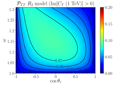
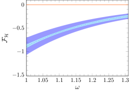
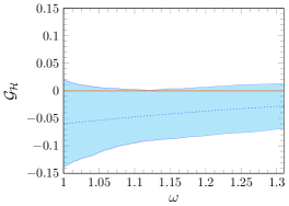
Figure 1: Results for $\Lambda_{b}\to\Lambda_{c}\tau\bar{\nu}_{\tau}$ evaluated with the $R_{2}$ leptoquark model of Ref. Shi:2019gxi , for which the two nonzero Wilson coefficients ($C^{S}_{LL}$ and $C^{T}_{LL}$) are complex. The unconstrained sign of ${\rm Im\,}[\hat{C}_{T}(1\,{\rm TeV})]$ is taken to be positive. The alternative choice ${\rm Im\,}[\hat{C}_{T}(1\,{\rm TeV})]<0$ would not change the absolute values of the observables shown in this figure, but only their global signs. Top: Two dimensional CM/LAB ${\cal P}_{TT}$ polarization (Eq. (48)) as a function of $\omega$ and the CM $\cos\theta_{\tau}$ variable. The polarization component is obtained using the central values for the form factors (see details in Sec. 4 below or in Ref. Penalva:2021gef ) and Wilson coefficients. Bottom: ${\cal F_{H}}(\omega)$ (left) and ${\cal G_{H}}(\omega)$ (right) scalar functions entering in the definition of the CP-violating ${\cal N_{H_{\rm 3}}}$ term of the differential decay width (Eqs. (14) and (15)). The error inherited from the form-factor uncertainties is evaluated and propagated via Monte Carlo, taking into account statistical correlations between the different parameters, and it is depicted as an inner band that accounts for 68% confident-level intervals. The uncertainty induced by the fitted Wilson coefficients is determined using different $1\sigma$ statistical samples configurations by the authors of Ref. Shi:2019gxi . The two sets of errors are then added in quadrature giving rise to the larger uncertainty band. Note that uncertainties on ${\cal G_{H}}(\omega)$ are largely dominated by the errors due to the form-factors.

Appropriate $\theta_{d}^{*}$ and/or $\phi^{*}_{d}$ asymmetries can be used to determine the longitudinal and the two transverse components of the tau-polarization four vector, which are two-dimensional functions of the variables $\omega$ and $s_{13}$ Penalva:2021gef . The observable $P_{TT}$ is of great interest, since it is given by the CP odd term ${\cal N_{H_{\rm 3}}}$ of the ${\cal P}^{\mu}$ decomposition in Eq. (18), which to be different from zero requires the existence of relative complex phases between Wilson coefficients. This component, transverse to the plane formed by the outgoing hadron and tau, could be obtained integrating over $\cos\theta_{d}^{*}$ and looking at the $\phi_{d}^{*}$ asymmetry

$$P_{TT}(\omega,s_{13}) = -\frac{2g^{d}}{g^{d}_{P}}\,\frac{\int_{0}^{\pi}d\phi_{d}^{*}\frac{d^{3}\Gamma_{d}}{d\omega ds_{13}d\phi_{d}^{*}}-\int_{\pi}^{2\pi}d\phi_{d}^{*}\frac{d^{3}\Gamma_{d}}{d\omega ds_{13}d\phi_{d}^{*}}}{\int_{0}^{\pi}d\phi_{d}^{*}\frac{d^{3}\Gamma_{d}}{d\omega ds_{13}d\phi_{d}^{*}}+\int_{\pi}^{2\pi}d\phi_{d}^{*}\frac{d^{3}\Gamma_{d}}{d\omega ds_{13}d\phi_{d}^{*}}}.$$ (48)

The projection ${\cal P}_{TT}$ is invariant under co-linear boost transformations, and thus it is the same in both CM and LAB systems. Measuring a non-zero ${\cal P}_{TT}$ value in any of these sequential decays will be a clear indication of physics BSM and of time reversal (or CP) violation. One can proceed similarly to obtain $P_{T}$ and $P_{L}$.

Upon integration on $s_{13}$, the semileptonic $d\Gamma_{\rm SL}/d\omega$ differential decay width can be factorized out in Eq. (47) by replacing the two-dimensional polarization components $P_{a}(\omega,s_{13})$ by averages on the $s_{13}$ variable weighted by the semileptonic distribution

$$P_{a}(\omega,s_{13})\to\langle P_{a}\rangle(\omega)=\left(\frac{d\Gamma_{\rm SL}}{d\omega}\right)^{-1}\int ds_{13}\frac{d^{2}\Gamma_{\rm SL}}{d\omega ds_{13}}P_{a}(\omega,s_{13}),\quad a=L,T,TT.$$ (49)

The $d^{3}\Gamma_{d}/(d\omega d\cos\theta^{*}_{d}d\phi_{d}^{*})$ distributions thus obtained coincide with the results given in Ref. Ivanov:2017mrj for the CM frame (center of mass system of the $\tau\bar{\nu}_{\tau}$ pair).

Both the two-dimensional and the averaged polarization components in the CM and LAB frames were detailedly studied, in Ref. Penalva:2021gef , in the presence of NP involving only left-handed neutrino operators. Results were obtained for the $\Lambda_{b}\to\Lambda_{c}\tau\bar{\nu}_{\tau}$, $\bar{B}_{c}\to\eta_{c}\tau\bar{\nu}_{\tau}$, $\bar{B}_{c}\to J/\psi\tau\bar{\nu}_{\tau}$ and $\bar{B}\to D^{(*)}\tau\nu_{\tau}$ decays, and in the case of the baryon decay, an special attention to BSM signatures derived from complex NP contributions was paid. We complete here the analysis of section 4.2.1 of Ref. Penalva:2021gef for the $\Lambda_{b}\to\Lambda_{c}\tau\bar{\nu}_{\tau}$ decay by showing in Fig. 1, the CP-violating observables ${\cal P}_{TT}(\omega,\cos\theta_{\tau})$ $\left(=-{\cal P}\cdot N_{TT}^{\rm LAB/CM}\right)$, ${\cal F_{H}}(\omega)$ and ${\cal G_{H}}(\omega)$ (see Eqs. (14) and (15)) obtained within the leptoquark model Shi:2019gxi employed in that section, and which predicts complex Wilson coefficients. The polarization $\langle P_{TT}\rangle(\omega)$ displayed in the left-bottom plot of Fig. 10 of Subsec. 4.2.1 of Ref. Penalva:2021gef can be obtained from the average indicated in Eq. (49) using the two-dimensional ${\cal P}_{TT}$ shown in the top plot of Fig. 1, and which could be measured by looking at the azimuthal asymmetry proposed in Eq. (48). This average $\langle P_{TT}\rangle(\omega)$ will be a linear combination of the ${\cal F_{H}}(\omega)$ and ${\cal G_{H}}(\omega)$ scalar functions, also displayed here in Fig. 1, which encode the maximal information contained in the CP-violating ${\cal N_{H_{\rm 3}}}$ term of the $\Lambda_{b}\to\Lambda_{c}\tau\bar{\nu}_{\tau}$ differential decay width. One cannot determine ${\cal F_{H}}(\omega)$ and ${\cal G_{H}}(\omega)$ only from $\langle P_{TT}\rangle(\omega)$. Therefore, to extract both of them, it would be necessary to analyze the dependence of the $d^{3}\Gamma_{d}/(d\omega d\cos\theta_{\tau}d\phi_{d}^{*})$ sequential decay distribution on $\phi^{*}_{d}$, which will allow to obtain the two-dimensional ${\cal P}_{TT}(\omega,\cos\theta_{\tau})$ polarization component.

3.4 Visible pion/rho/muon variables in the CM frame.

When the tau momentum cannot be fully reconstructed experimentally, the previous expressions are no longer useful, since the kinematics of the decay-product is referred to the $\tau$ direction. It is therefore suitable to construct observables directly from final-state kinematics of the visible decay particle $\pi,\rho,\mu$, without relying on the reconstruction of the tau momentum, which needs to be integrated out ($s_{13})$. We take the energy of the charged particle in the $\tau-$decay, $E_{d}$ and its angle $\theta_{d}$ with the final hadron $H_{c}$, both variables defined in the CM frame ($\vec{q}=0$, $W$ boson at rest). This kinematical set up has been extensively used in the literature to analyze NP signatures in $\bar{B}\to D^{(*)}\tau\,(\pi\nu_{\tau},\rho\nu_{\tau},\mu\bar{\nu}_{\mu}\nu_{\tau})\bar{\nu}_{\tau}$ decays Kiers:1997zt ; Nierste:2008qe ; Alonso:2016gym ; Alonso:2017ktd ; Asadi:2020fdo , although these studies have not considered BSM right-handed neutrino fields. Moreover, a similar polarimetry analysis for the $\Lambda_{b}\to\Lambda_{c}\tau\bar{\nu}_{\tau}$ reaction has not be done yet, despite the good prospects that LHCb can measure it in the near future, given the large number of $\Lambda_{b}$ baryons which are produced at LHC.

Following the notation in Ref Tanaka:2010se , we introduce

$$\gamma=\frac{q^{2}+m^{2}_{\tau}}{2m_{\tau}\sqrt{q^{2}}},\quad\beta=\frac{\sqrt{\gamma^{2}-1}}{\gamma}=\frac{q^{2}-m^{2}_{\tau}}{q^{2}+m^{2}_{\tau}},\quad\xi_{d}=\frac{E_{d}}{m_{\tau}\gamma},$$ (50)

with $\gamma$ and $\beta$ defining the boost from the $\tau$ rest frame to the CM one. In addition, the dimensionless variable $\xi_{d}$ is the CM ratio of the energies of the tau-decay massive product and the tau lepton. Let us call now $\theta_{\tau d}^{\rm CM}\in[0,\pi[$, the angle formed by the $\vec{p}_{\tau}$ and $\vec{p}_{d}$ in the CM reference system. We have

$$\tau\to(\pi,\rho)\nu_{\tau} \Rightarrow (\cos\theta_{\tau d}^{\rm CM})(\omega,\xi_{d})=\frac{2\gamma\xi_{d}-(1+y^{2})/\gamma}{2\beta\sqrt{\gamma^{2}\xi_{d}^{2}-y^{2}}},$$

$$\tau\to\mu\bar{\nu}_{\mu}\nu_{\tau} \Rightarrow (\cos\theta_{\tau d}^{\rm CM})(\omega,\xi_{d},x)=\frac{2\gamma\xi_{d}-x/\gamma}{2\beta\sqrt{\gamma^{2}\xi_{d}^{2}-y^{2}}},$$ (51)

where we have used $y=m_{d}/m_{\tau}$ for all decay modes. For the hadronic channels $\cos\theta_{\tau d}^{\rm CM}$, obtained in that case from the condition $(k^{\prime}-p_{d})^{2}=0$, is totally fixed by $\omega$ and the energy of the tau-decay massive product, while for the lepton mode it also depends on the additional variable $x=2(p_{\mu}\cdot k^{\prime})/m^{2}_{\tau}$ introduced above. Next, requiring $(\cos\theta_{\tau d}^{\rm CM})^{2}\leq 1$, we obtain the allowed region for the energy of the pion or rho mesons

$$\tau\to(\pi,\rho)\nu_{\tau} \Rightarrow \frac{1-\beta}{2}+\frac{1+\beta}{2}y^{2}=\xi_{1}\leq\xi_{d}\leq\xi_{2}=\frac{1+\beta}{2}+\frac{1-\beta}{2}y^{2},$$ (52)

or bounds that the variable $x$ should satisfy in the lepton mode,

$$\tau\to\mu\bar{\nu}_{\mu}\nu_{\tau} \Rightarrow x_{-}\leq x\leq x_{+},\quad x_{\pm}=2\gamma^{2}\xi_{d}\pm 2\gamma\beta\sqrt{\gamma^{2}\xi_{d}^{2}-y^{2}}.$$ (53)

Also for this latter case, the maximum allowed value of $\xi_{d}$ is still $\xi_{2}$, which corresponds to $E_{d}^{\rm max}=(q^{2}+m_{d}^{2})/(2\sqrt{q^{2}})$. However, in certain circumstances, $\xi_{d}$ can be as low as $y/\gamma$ for all reachable $q^{2}$. This is to say a kinematics where the daughter massive lepton is at rest in the CM frame, which would be compatible with the energy-momentum conservation thanks to the other two neutrinos present in the tau-decay final state. In general, one finds

$$y\leq\sqrt{\frac{1-\beta}{1+\beta}}=\frac{m_{\tau}}{\sqrt{q^{2}}} \Rightarrow y/\gamma\leq\xi_{d}\leq\xi_{2},$$ (54)

$$y>\sqrt{\frac{1-\beta}{1+\beta}}=\frac{m_{\tau}}{\sqrt{q^{2}}} \Rightarrow \xi_{1}\leq\xi_{d}\leq\xi_{2}.$$ (55)

For the $b\to c$ semileptonic decays analyzed here, we have $y=m_{\mu}/m_{\tau}$ and $\sqrt{q^{2}}\leq(M-M^{\prime})<m^{2}_{\tau}/m_{\mu}$, which corresponds to the range of Eq. (54). Thus, the outgoing muon can exit at rest for any $q^{2}$ value, fixing in this way the minimum reachable value for $\xi_{d}$ to $y/\gamma$ ($E_{d}=m_{\mu})$ independently of $q^{2}$ (or $\omega$). In a hypothetical case, for which $y^{2}>(1-\beta)/(1+\beta)$ (Eq. (55)), the outgoing massive particle could not exit with zero momentum.

The bounds of Eq. (53) should be combined with the product of step functions $H(x-2y)H(1+y^{2}-x)$ which appears in the definition of $\eta_{d=\mu\bar{\nu}_{\mu}}$ and $\chi_{d=\mu\bar{\nu}_{\mu}}$ in Eqs. (41) and (43), respectively. While $2y$ is always smaller than the lower bound in Eq. (53), the combined use of $(1+y^{2})$ and the upper bound $x_{+}$ is more subtle and it leads to the following available phase space

$$y\leq\sqrt{\frac{1-\beta}{1+\beta}} \Rightarrow \varphi(\omega,\xi_{d},x)=H(\xi_{d}-y/\gamma)H(\xi_{1}-\xi_{d})H(x-x_{-})H(x_{+}-x)$$ (56)

$$+H(\xi_{d}-\xi_{1})H(\xi_{2}-\xi_{d})H(x-x_{-})H(1+y^{2}-x),$$

$$y>\sqrt{\frac{1-\beta}{1+\beta}} \Rightarrow \widetilde{\varphi}(\omega,\xi_{d},x)=H(\xi_{d}-\xi_{1})H(\xi_{2}-\xi_{d})H(x-x_{-})H(1+y^{2}-x),$$ (57)

in agreement with the results of Ref Tanaka:2010se obtained for $y=0$.

Taking in this case the outgoing hadron momentum $\vec{p}^{\,\prime}$ as the positive $Z$ direction and $\vec{p}\,^{\prime}\times\vec{k}\,^{\prime}$ as the positive $Y$ direction, one can write $k^{\prime\mu}=m_{\tau}\gamma(1,\beta\sin\theta_{\tau},0,\beta\cos\theta_{\tau})$ and

$$\cos\theta_{\tau d}^{\rm CM}=\sin\theta_{\tau}\sin\theta_{d}\cos\phi_{d}+\cos\theta_{\tau}\cos\theta_{d}\Rightarrow\cos\phi_{d}=\frac{\cos\theta_{\tau d}^{\rm CM}-\cos\theta_{\tau}\cos\theta_{d}}{\sin\theta_{\tau}\sin\theta_{d}}=z_{0},$$ (58)

with $\theta_{d}$ and $\phi_{d}$ the polar and azimuthal angles of the three-momentum $\vec{p}_{d}$ in the CM frame, $\vec{p}_{d}=m_{\tau}\sqrt{\gamma^{2}\xi_{d}^{2}-y^{2}}\left(\sin\theta_{d}\cos\phi_{d},\sin\theta_{d}\sin\phi_{d},\cos\theta_{d}\right)$. The variable $z_{0}$ above depends on $\omega$ and $\cos\theta_{\tau}$ for the hadron modes, while it also depends on $x$, through $\cos\theta_{\tau d}^{\rm CM}$, in the lepton channel. The condition $(\cos\phi_{d})^{2}\leq 1$ limits the values of the cosinus of the CM $\tau$-polar angle to the range

$$\cos(\theta_{d}+\theta_{\tau d}^{\rm CM})\leq\cos\theta_{\tau}\leq\cos(\theta_{d}-\theta_{\tau d}^{\rm CM}).$$ (59)

In addition, we can express the scalar product $(p_{d}\cdot{\cal P}(\omega,s_{13}))$ in terms of the CM-variables as:

$$\frac{(p_{d}\cdot{\cal P})}{m_{\tau}} = \gamma\left(\gamma\beta\xi_{d}-\sqrt{\gamma^{2}\xi_{d}^{2}-y^{2}}\cos\theta_{\tau d}^{\rm CM}\right)P_{L}^{\rm CM}(\omega,\cos\theta_{\tau})$$ (60)

$$+\sqrt{\gamma^{2}\xi_{d}^{2}-y^{2}}\Big{\{}P_{TT}^{\rm CM}(\omega,\cos\theta_{\tau})\sin\theta_{d}\sin\phi_{d}$$

$$+\frac{P_{T}^{\rm CM}(\omega,\cos\theta_{\tau})}{\sin\theta_{\tau}}\left[\cos\theta_{\tau}\cos\theta_{\tau d}^{\rm CM}-\cos\theta_{d}\right]\Big{\}},$$

where we have used ${\cal P}^{\mu}=\left(P_{L}N_{L}^{\mu}+P_{T}N_{T}^{\mu}+P_{TT}N_{TT}^{\mu}\right)_{\rm CM}$, with the vectors $N_{L,T,TT}^{\mu}$ computed using Eq. (46), the CM final hadron and tau four momenta and the relations $P_{L,T,TT}=-({\cal P}\cdot N_{L,T,TT})$ (see Ref. Penalva:2021gef for further details). We recall that in Eq. (60), the definition of $\cos\theta_{\tau d}^{\rm CM}$ involves $\cos\phi_{d}$ (see Eq. (58)).

Taking into account the dependence of $(p\cdot k),(p\cdot N_{L,T}^{\rm CM})$ and $(q\cdot N_{L,T}^{\rm CM})$ on $\cos\theta_{\tau}$, ones finds Penalva:2021gef (the $P_{TT}^{\rm CM}$ term will not contribute after integrating in $\phi_{d}$)

$$P_{L}^{\rm CM}(\omega,\cos\theta_{\tau}) = \frac{\delta a_{0}(\omega)+\delta a_{1}(\omega)\cos\theta_{\tau}+\delta a_{2}(\omega)\cos^{2}\theta_{\tau}}{a_{0}(\omega)+a_{1}(\omega)\cos\theta_{\tau}+a_{2}(\omega)\cos^{2}\theta_{\tau}},$$

$$\frac{P_{T}^{\rm CM}(\omega,\cos\theta_{\tau})}{\sin\theta_{\tau}} = \frac{p^{\prime}_{0}(\omega)+p^{\prime}_{1}(\omega)\cos\theta_{\tau}}{a_{0}(\omega)+a_{1}(\omega)\cos\theta_{\tau}+a_{2}(\omega)\cos^{2}\theta_{\tau}},$$ (61)

where, for $i=1,2,3$, one has

$$\delta a_{i}(\omega)=a_{i}(\omega,h=-1)-a_{i}(\omega,h=+1),$$

$$a_{i}(\omega)=a_{i}(\omega,h=-1)+a_{i}(\omega,h=+1),$$ (62)

which are functions of ${\cal A_{H}},{\cal B_{H}},{\cal C_{H}},{\cal D_{H}}$ and ${\cal E_{H}}$ and ${\cal A},{\cal B}$ and ${\cal C}$ respectively (see Eqs. (14), (15) and (16) ). Besides,

$$p^{\prime}_{0}(\omega)=\frac{M^{\prime}\sqrt{\omega^{2}-1}}{M\sqrt{q^{2}}}\left(\frac{2M{\cal A_{H}}(\omega)}{1-m^{2}_{\tau}/q^{2}}+M_{\omega}{\cal C_{H}}(\omega)\right),\quad p^{\prime}_{1}(\omega)=\frac{M^{\prime\,2}(\omega^{2}-1)}{M\sqrt{q^{2}}}{\cal C_{H}}(\omega).$$ (63)

Now, we are in conditions to address the integration of the $\phi_{d}$ and $\cos\theta_{\tau}$ (or $s_{13}$),

• For the hadronic modes, the $\eta_{d=\mu\bar{\nu}_{\mu}}$ and $\chi_{d=\mu\bar{\nu}_{\mu}}$ functions contain an energy conservation Dirac delta function, which can be used to integrate $d\phi_{d}$,

  $$\frac{\delta\big{[}\sqrt{m_{\tau}^{2}+\vec{k}^{\,\prime\,2}}-\sqrt{m_{d}^{2}+\vec{p}_{d}^{\,2}}-|\vec{k^{\prime}}-\vec{p}_{d}|\big{]}}{|\vec{k^{\prime}}-\vec{p}_{d}|}=\frac{\delta\left(\cos\phi_{d}-z_{0}\right)}{|\vec{k^{\prime}}||\vec{p}_{d}|\sin\theta_{\tau}\sin\theta_{d}},$$ (64)

  with $z_{0}$ introduced in Eq. (58). Now, we use

  $$\int_{0}^{2\pi}d\phi_{d}\,\delta\left(\cos\phi_{d}-z_{0}\right)g\left(\cos\phi_{d},\sin\phi_{d}\right) = \int_{-1}^{1}dz\frac{\delta(z-z_{0})}{\sqrt{1-z^{2}}}\Big{[}g\left(z,\sqrt{1-z^{2}}\right)$$ (65)

  $$+g\left(z,-\sqrt{1-z^{2}}\right)\Big{]}$$

  to carry out the $\phi_{d}$ integration. As a result, we find that the $P_{TT}$ contribution vanishes and considering $\sin\theta_{\tau}\sin\theta_{d}$ in Eq. (64), we obtain a common factor

  $$\frac{1}{\sin\theta_{\tau}\sin\theta_{d}\sqrt{1-z^{2}_{0}}}=\frac{1}{\sqrt{\left[\cos(\theta_{d}-\theta_{\tau d}^{\rm CM})-\cos\theta_{\tau}\right]\left[\cos\theta_{\tau}-\cos(\theta_{d}+\theta_{\tau d}^{\rm CM})\right]}}.$$ (66)

  Now, the integration over $\cos\theta_{\tau}$ can be easily done using the analytical integrals compiled in Eq. (112), which appear when the factor from the above equation, the longitudinal and transverse polarization components given in Eq. (61), the expression for the CM $d^{2}\Gamma_{SL}/(d\omega d\cos\theta_{\tau})$ in Eq. (16) and the limits of Eq. (59) are considered.

• In the leptonic mode, the $\eta_{d=\mu\bar{\nu}_{\mu}}$ and $\chi_{d=\mu\bar{\nu}_{\mu}}$ functions do not contain any Dirac delta. However, many of the results of the previous case can also be used here. To fix the OXZ plane, it is necessary to detect both the hadron and tau momenta, and given the expected experimental difficulties to reconstruct the $\tau$-trajectory, we integrate the azimuthal $\phi_{d}$ angle. It holds

  $$\int_{0}^{2\pi}d\phi_{d}\,g\left(\cos\phi_{d},\sin\phi_{d}\right) = \int_{-1}^{1}dz_{0}\frac{g\left(z_{0},\sqrt{1-z_{0}^{2}}\right)+g\left(z_{0},-\sqrt{1-z_{0}^{2}}\right)}{\sqrt{1-z_{0}^{2}}}.$$ (67)

  Here, we see again that the contribution of the CP-violating polarization component $P_{TT}$ cancels out, and some kind of $\phi_{d}$-asymmetry, similar to that of Eq. (48), would be needed to isolate this term. In addition, $z_{0}=z_{0}(x)$ and the change of variables

  $$dz_{0}=\frac{dx}{|\partial x/\partial z_{0}|}=\frac{dx}{2\gamma\beta\sqrt{\gamma^{2}\xi_{d}^{2}-y^{2}}\sin\theta_{\tau}\sin\theta_{d}}$$ (68)

  completes the reconstruction of the factor of Eq. (66). Altogether, we can integrate $d\cos\theta_{\tau}$ in a similar way to what we have shown above in detail for the hadronic channel. The main difference is that to obtain the $d^{3}\Gamma_{d}/(d\omega d\xi_{d}d\cos\theta_{d})$ distribution of visible variables, we still have to integrate over the $x$ variable, taking into account the accessible phase-space $\varphi(\omega,\xi_{d},x)$ given in Eq. (56).

Thus, finally we obtain for $y^{2}\leq m_{\tau}^{2}/\sqrt{q^{2}}$

$$\frac{d^{3}\Gamma_{d}}{d\omega d\xi_{d}d\cos\theta_{d}} = {\cal B}_{d}\frac{d\Gamma_{\rm SL}}{d\omega}\Big{\{}F^{d}_{0}(\omega,\xi_{d})+F^{d}_{1}(\omega,\xi_{d})\cos\theta_{d}+F^{d}_{2}(\omega,\xi_{d})P_{2}(\cos\theta_{d})\Big{\}},$$ (69)

with $P_{2}$ the Legendre polynomial of order two. The contributions of the different waves for the hadronic modes read

$$F^{\pi,\rho}_{0}(\omega,\xi_{d}) = \frac{1}{2\beta(1-y^{2})}\,\left(1+\frac{a_{\pi,\rho}\left(1+y^{2}-2\xi_{d}\right)}{\beta(1-y^{2})}\,\langle P_{L}^{\rm CM}\rangle(\omega)\right),$$

$$F^{\pi,\rho}_{1}(\omega,\xi_{d}) = \frac{3}{2\beta(1-y^{2})}\,\Bigg{\{}\frac{a_{1}\cos\theta_{\tau d}^{\rm CM}}{3a_{0}+a_{2}}+\frac{a_{\pi,\rho}}{1-y^{2}}\Bigg{(}\frac{1+y^{2}-2\xi_{d}}{\beta}\frac{\delta a_{1}}{3a_{0}+a_{2}}\cos\theta_{\tau d}^{\rm CM}$$

$$-\frac{8\sqrt{\gamma^{2}\xi_{d}^{2}-y^{2}}}{3\pi}\left[\sin\theta_{\tau d}^{\rm CM}\right]^{2}\langle P_{T}^{\rm CM}\rangle\Bigg{)}\Bigg{\}},$$

$$F^{\pi,\rho}_{2}(\omega,\xi_{d}) = \frac{1}{\beta(1-y^{2})}\,\Bigg{\{}\frac{a_{2}}{3a_{0}+a_{2}}P_{2}(\cos\theta_{\tau d}^{\rm CM})+\frac{a_{\pi,\rho}}{1-y^{2}}\Bigg{(}\frac{1+y^{2}-2\xi_{d}}{\beta}\frac{\delta a_{2}}{3a_{0}+a_{2}}P_{2}(\cos\theta_{\tau d}^{\rm CM})$$ (70)

$$-\sqrt{\gamma^{2}\xi_{d}^{2}-y^{2}}\left[\sin\theta_{\tau d}^{\rm CM}\right]^{2}\cos\theta_{\tau d}^{\rm CM}\frac{3p^{\prime}_{1}}{3a_{0}+a_{2}}\Bigg{)}\Bigg{\}}.$$

For the lepton channel, for which we remind that $\cos\theta_{\tau d}^{\rm CM}$ depends also on the integration variable $x$, we have

$$F^{\mu\bar{\nu}_{\mu}}_{0}(\omega,\xi_{d}) = \frac{1}{\beta f(y)}\int dx\,\varphi(\omega,\xi_{d},x)\Big{\{}G_{1}(x,y)+\langle P_{L}^{\rm CM}\rangle(\omega)G_{L}(x,y)\Big{\}},$$

$$F^{\mu\bar{\nu}_{\mu}}_{1}(\omega,\xi_{d}) = \frac{3}{\beta f(y)}\int dx\,\varphi(\omega,\xi_{d},x)\Bigg{\{}\frac{a_{1}(\omega)G_{1}(x,y)+\delta a_{1}(\omega)G_{L}(x,y)}{3a_{0}(\omega)+a_{2}(\omega)}\cos\theta_{\tau d}^{\rm CM}$$

$$-\frac{8\sqrt{\gamma^{2}\xi_{d}^{2}-y^{2}}\,}{3\pi}\langle P_{T}^{\rm CM}\rangle(\omega)\left[\sin\theta_{\tau d}^{\rm CM}\right]^{2}G_{T}(x,y)\Bigg{\}},$$

$$F^{\mu\bar{\nu}_{\mu}}_{2}(\omega,\xi_{d}) = \frac{2}{\beta f(y)}\int dx\,\varphi(\omega,\xi_{d},x)\Bigg{\{}\frac{a_{2}(\omega)G_{1}(x,y)+\delta a_{2}(\omega)G_{L}(x,y)}{3a_{0}(\omega)+a_{2}(\omega)}P_{2}(\cos\theta_{\tau d}^{\rm CM})$$ (71)

$$-\sqrt{\gamma^{2}\xi_{d}^{2}-y^{2}}\frac{3p^{\prime}_{1}(\omega)}{3a_{0}(\omega)+a_{2}(\omega)}\left[\sin\theta_{\tau d}^{\rm CM}\right]^{2}\cos\theta_{\tau d}^{\rm CM}G_{T}(x,y)\Bigg{\}},$$

with the functions $G_{1}(x,y)=x(3-2x)-y^{2}(4-3x)$, $G_{L}(x,y)=\left(x-2\xi_{d}\right)\left(1+3y^{2}-2x\right)/\beta$ and $G_{T}(x,y)=\left(1+3y^{2}-2x\right)$. The integrations on the variable $x$ are straightforward in all cases since only polynomials are involved. The actual expressions, lengthy ones in some cases, have been collected in Appendix G where we also provide, more visual, two-dimensional graphic representations of their $(\omega,\xi_{d})$ dependence.

Note that $G_{1}$ and $G_{L}$ provide the overall normalization

$$\frac{2}{\beta f(y)}\int d\xi_{d}\int dx\varphi(\omega,\xi_{d},x)G_{1}(x,y)=1,\quad\int d\xi_{d}\int dx\varphi(\omega,\xi_{d},x)G_{L}(x,y)=0,$$ (72)

where the equivalent ones for the hadronic modes are trivially satisfied. Upon integration on $\cos\theta_{d}$, and taking the massless limit $y\to 0$, we recover the results of Ref. Tanaka:2010se identifying $2F^{d}_{0}(\omega,\xi_{d})$ here with $f(q^{2},\xi)+P_{L}(q^{2})g(q^{2},\xi)$ in that reference. Note that, besides some differences in the notation, there is a sign change in the definition of the polarization terms we provide here with respect to the ones in Refs. Tanaka:2010se ; Alonso:2016gym .

In the sequential $\tau$-decay distribution of Eq. (69), all information on the $b\to c\tau\bar{\nu}_{\tau}$ transition is encoded in the $\omega$-dependent functions $a_{i},\delta a_{i},p^{\prime}_{1}$ and $\langle P^{\rm CM}_{L,T}\rangle$. As already mentioned, they can be expressed in terms of the ${\cal A},{\cal B}$ and ${\cal C}$ and ${\cal A_{H}},{\cal B_{H}},{\cal C_{H}},{\cal D_{H}}$ and ${\cal E_{H}}$ ones introduced here in Eqs. (14) and (15). The first set of three functions (or equivalently $a_{0,1,2}$) determine the unpolarized $H_{b}\to H_{c}\tau\bar{\nu}_{\tau}$ semileptonic $d^{2}\Gamma_{SL}/(d\omega d\cos\theta_{\tau})$ distribution. The helicity-asymmetry coefficients $\delta a_{i=0,1,2}(\omega)$ involve only the second set of functions, while $p^{\prime}_{1}$ only involves ${\cal C_{H}}$. Finally, the angular weighted averages of the longitudinal and transverse components of the tau polarization vector are exhaustively discussed in Ref. Penalva:2021gef , where (Appendix B) analytical expressions in terms of ${\cal A_{H}},{\cal B_{H}},{\cal C_{H}},{\cal D_{H}}$ and ${\cal E_{H}}$ and the combination $(3a_{0}+a_{2})$, can be found. Note also that $\langle P^{\rm CM}_{L}\rangle=\frac{3\delta a_{0}+\delta a_{2}}{3a_{0}+a_{2}}$ and $\langle P^{\rm CM}_{T}\rangle=\frac{3\pi p^{\prime}_{0}}{4(3a_{0}+a_{2})}$. Thus for fixed $\omega$, the combined $(\xi_{d},\cos\theta_{d}$) analysis of the $d^{3}\Gamma_{d}/(d\omega d\xi_{d}d\cos\theta_{d})$ distribution provides, in addition to $a_{0}$, $a_{1}$ and $a_{2}$, five independent observables $\delta a_{i=0,1,2}(\omega)$, $\langle P^{\rm CM}_{T}\rangle$ and $p^{\prime}_{1}$, which can be used to fully determine the five ${\cal A_{H}},{\cal B_{H}},{\cal C_{H}},{\cal D_{H}}$ and ${\cal E_{H}}$ $\omega$-functions, and that give the maximal information on NP in the $b\to c\tau\bar{\nu}_{\tau}$ transition, without considering CP-violation. CP non-conserving contributions, encoded in the $P_{TT}$ component of the tau polarization vector, canceled out when we carried out the $\phi_{d}$ integration. As noted above, the measurement of such angle would require to detect the $\tau$-three momentum. Hence, the ${\cal F_{H}}$ and ${\cal G_{H}}$ functions, which are responsible for CP violation, are only accessible by including additional information. For $\bar{B}\to D^{*}$, some CP-odd observables (triple product asymmetries), defined using angular distributions involving the kinematics of the products of the $D^{*}$ decay, have also been presented Duraisamy:2013pia ; Duraisamy:2014sna ; Ligeti:2016npd ; Bhattacharya:2020lfm . These asymmetries are sensitive to the relative phases of the Wilson coefficients, as are the ${\cal F_{H}}$ and ${\cal G_{H}}$ scalar functions.

We note that the expression found here for the visible distribution in Eq. (69) recovers the results presented in Refs. Alonso:2016gym ; Alonso:2017ktd ; Asadi:2020fdo for $\bar{B}\to D^{(*)}$ transitions, accounting in the leptonic mode also for effects due to the finite mass of the outgoing muon/electron from the tau decay. Thus, there is a correspondence between $n(q^{2})$ and the asymmetries $A_{FB},P_{L},P_{\perp},Z_{L},Z_{\perp},Z_{Q}$ and $A_{Q}$ introduced in Eq. (1.1) of Ref. Asadi:2020fdo for the hadron modes, and $a_{i=0,1,2}$, $\delta a_{i=0,1,2},p^{\prime}_{1}$ and $\langle P^{\rm CM}_{T}\rangle$ (or ${\cal A},{\cal B}$ and ${\cal C}$, and ${\cal A_{H}},{\cal B_{H}},{\cal C_{H}},{\cal D_{H}}$ and ${\cal E_{H}}$) used here. In fact, the relationships become apparent when comparing equations (3.12) and (3.13) of Asadi:2020fdo and the Eqs. (69)-(70) in this work,

$$n(q^{2}) \propto \left(3a_{0}(\omega)+a_{2}(\omega)\right),\quad A_{FB}(q^{2})=\frac{3a_{1}(\omega)/2}{3a_{0}(\omega)+a_{2}(\omega)},\quad A_{Q}(q^{2})=\frac{a_{2}(\omega)}{3a_{0}(\omega)+a_{2}(\omega)}$$

$$P_{L}(q^{2}) = -\langle P^{\rm CM}_{L}\rangle,\quad Z_{L}(q^{2})=-\frac{3\delta a_{1}(\omega)/2}{3a_{0}(\omega)+a_{2}(\omega)},\quad Z_{Q}(q^{2})=-\frac{\delta a_{2}(\omega)}{3a_{0}(\omega)+a_{2}(\omega)}$$

$$P_{\perp}(q^{2}) = -\langle P^{\rm CM}_{T}\rangle,\quad Z_{\perp}(q^{2})=-\frac{p^{\prime}_{1}(\omega)}{3a_{0}(\omega)+a_{2}(\omega)}.$$ (73)

Unpolarized $\tau$	$\mathcal{A},\,\mathcal{B},\,\mathcal{C}$	$n,\,A_{{FB}},\,A_{Q}$
Polarized $\tau$	$\mathcal{A_{H}},\,\mathcal{B_{H}},\,\mathcal{C_{H}},\,\mathcal{D_{H}},\,\mathcal{E_{H}}$	$\langle P_{L}^{\rm CM}\rangle,\,\langle P_{T}^{\rm CM}\rangle,\,Z_{L},\,Z_{Q},\,Z_{\perp}$
Polarized $\tau$, complex Wilson coeff.	$\mathcal{F_{H}},\,\mathcal{G_{H}}$	$\langle P_{TT}\rangle,\,\ Z_{T}$

Table 1: For each row, the observables in the second column contain the same physical information as those compiled in the third one. The quantities in the first row determine the decay for unpolarized taus, while the ones in the second and third rows describe the decays for polarized taus. Finally, observables in the third row are zero unless the Wilson coefficients are complex.

In addition, the remaining two asymmetries $P_{T}$ (related to our $\langle P_{TT}\rangle$) and $Z_{T}$ mentioned in Asadi:2020fdo should correspond to linear combinations of the ${\cal F_{H}}$ and ${\cal G_{H}}$ scalar functions within the tensor formalism presented in Sec. 2. As mentioned above, these CP-violating contributions cancel out on integration over the azimuthal angle $\phi_{d}$, which measurement would require detecting both the hadron and tau momenta. These relations are schematically shown in Table 1 where, for each row, the observables in the second and the third columns are equivalent in the sense that they contain the same physical information. In addition, we show which quantities determine the decay for unpolarized (first row) and polarized (second and third rows) final taus, as well as which of them require complex Wilson coefficients (third row).

As we have seen, the tensor scheme of Sec. 2 allows to straightforwardly compute the $d^{3}\Gamma_{d}/(d\omega d\xi_{d}d\cos\theta_{d})$ distribution of visible variables for any $H_{b}\to H_{c}\tau\,(d\nu_{\tau})\bar{\nu}_{\tau}$ decay, including left- and/or right-handed NP neutrino operators.

Each of the observables in Eq. (73), which are embedded in one of the $F^{d}_{0,1,2}(\omega,\xi_{d})$ partial waves introduced in Eq. (69), are affected by kinematical $C_{n},C_{A_{FB}},\dots,C_{Z_{\perp}}$ coefficients. Specifically, one can write

$$F^{d}_{0}(\omega,\xi_{d}) = C_{n}^{d}(\omega,\xi_{d})+C_{P_{L}}^{d}(\omega,\xi_{d})\,\langle P^{\rm CM}_{L}\rangle(\omega),$$

$$F^{d}_{1}(\omega,\xi_{d}) = C_{A_{FB}}^{d}(\omega,\xi_{d})A_{FB}(\omega)+C_{Z_{L}}^{d}(\omega,\xi_{d})Z_{L}(\omega)+C_{P_{T}}^{d}(\omega,\xi_{d})\,\langle P^{\rm CM}_{T}\rangle(\omega),$$

$$F^{d}_{2}(\omega,\xi_{d}) = C_{A_{Q}}^{d}(\omega,\xi_{d})A_{Q}(\omega)+C_{Z_{Q}}^{d}(\omega,\xi_{d})Z_{Q}(\omega)+C_{Z_{\perp}}^{d}(\omega,\xi_{d})Z_{\perp}(\omega).$$ (74)

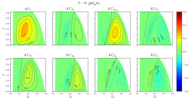
Figure 4: Same as Fig. 3 but for the $\mu\bar{\nu}_{\mu}$ tau-decay mode.

Those coefficients are tau-decay mode dependent and in the case of the $\pi$ and $\rho$ hadronic ones they can be easily read out from Eq. (70). The corresponding expressions for the fully $\mu\bar{\nu}_{\mu}$ leptonic mode are collected in Appendix  G. There, in Figs. 3 and 4, we also provide, for all three tau-decay modes considered in this work, their $(\omega,\xi_{d})$-graphic representations. What we actually show are the products of each of the coefficients times the kinematical factor ${\cal K}(\omega)=\sqrt{\omega^{2}-1}\,(1-m_{\tau}^{2}/q^{2})^{2}$ that makes part of the $d\Gamma_{\rm SL}/d\omega$ semileptonic decay width. The visual inspection of the different panels in Figs. 3 and 4 provides immediate information on which regions of the available $(\omega,\xi_{d})$ phase-space might result more sensitive to (or adequate to extract from) each of the observables of Eq. (73). Taking into account the numerical values of the coefficients, the hadron channels, and in particular the pion mode, seem, in general, to be more convenient to determine the semileptonic quantities of Eq. (73). Probably, the best strategy would be to perform a multi-parametric fit of the $d^{3}\Gamma_{d}/(d\omega d\xi_{d}d\cos\theta_{d})$ experimental data to the theoretical predictions of Eqs. (69)-(70).

4 Results for the visible pion/rho/muon distributions in the presence of NP right-handed neutrino operators

	SM	L Fit 7 Murgui:2019czp	R S3 Mandal:2020htr	R S5a Mandal:2020htr	R S7a Mandal:2020htr
$\Gamma_{e(\mu)}$	$2.15\pm 0.08$	$-$	$-$
$\Gamma_{\tau}$	$0.715\pm 0.015$	$0.89\pm 0.05$	$0.81\pm 0.04$	$0.81\pm 0.04$	$0.81\pm 0.06$
${\cal R}_{\Lambda_{c}}$	$0.332\pm 0.007$	$0.41\pm 0.02$	$0.378\pm 0.017$	$0.378\pm 0.017$	$0.38\pm 0.03$

Table 2: Total decay widths $\Gamma_{\tau}=\Gamma\left(\Lambda_{b}\to\Lambda_{c}\tau\bar{\nu}_{\tau}\right)$ and $\Gamma_{e(\mu)}=\Gamma\left(\Lambda_{b}\to\Lambda_{c}\,e(\mu)\bar{\nu}_{e(\mu)}\right)$ [units of $\left(10\times|V_{cb}|^{2}{\rm ps}^{-1}\right)$] and ratios ${\cal R}_{\Lambda_{c}}=\Gamma\left(\Lambda_{b}\to\Lambda_{c}\tau\bar{\nu}_{\tau}\right)/\Gamma\left(\Lambda_{b}\to\Lambda_{c}\,e(\mu)\bar{\nu}_{e(\mu)}\right)$ obtained in the SM, the NP model Fit 7 of Ref. Murgui:2019czp , which involves only left-handed neutrinos, and other three ones taken from Ref. Mandal:2020htr , where all included NP operators use right-handed neutrino fields (see text for details). Errors induced by the uncertainties in the form-factors and Wilson Coefficients are added in quadrature.

We will consider three different extensions of the SM including right-handed neutrino fields, that correspond to the more promising ones, in terms of the pulls from the SM hypothesis, among those discussed in Ref. Mandal:2020htr . We will show predictions for the observables collected in Eq. (73), extracted from the visible distributions of the tau-decay massive products, for the baryon $\Lambda_{b}\to\Lambda_{c}$ reaction. We will compare these NP results with those obtained in the SM, and within an extension of the SM determined by Fit 7 of Ref. Murgui:2019czp constructed only with left-handed neutrino operators. We focus in the baryon decay for the sake of brevity, since some of the observables of Eq. (73) with right-handed neutrinos were already shown in Mandal:2020htr for the meson $\bar{B}\to D^{(*)}$ semileptonic decays, where the extensions considered in this work were fitted. Moreover, $\bar{B}_{c}\to\eta_{c},J/\psi$ transitions, studied in our previous works, follow in general a similar pattern to that seen in the analog ones from $\bar{B}$-meson decays. In addition, we will not include results from Fit 6 of Ref. Murgui:2019czp , as we did in previous studies Penalva:2019rgt ; Penalva:2020xup ; Penalva:2020ftd ; Penalva:2021gef , since this NP scenario, which involves only left-handed neutrinos, provides polarized tau-distributions more similar to the SM ones than those obtained with the model Fit 7 of the same reference.

The $\Lambda_{b}\to\Lambda_{c}$ form factors used here are directly obtained (see Appendix E of Ref. Penalva:2020xup ) from those calculated in the lattice quantum Chromodynamics (LQCD) simulations of Refs. Detmold:2015aaa (vector and axial ones) and Datta:2017aue (tensor NP form factors) using $2+1$ flavors of dynamical domain-wall fermions. The NP scalar and pseudoscalar form factors are directly related to the vector and axial ones and we use Eqs. (2.12) and (2.13) of Ref. Datta:2017aue to evaluate them. We use the errors and statistical correlation-matrices, provided in the LQCD papers, to Monte Carlo transport the form-factor uncertainties to the different observables shown in this work. For the model Fit 7 and the right-handed neutrino scenarios, we shall use statistical samples of Wilson coefficients selected such that the $\chi^{2}$-merit function computed in Refs. Murgui:2019czp and Mandal:2020htr , respectively, changes at most by one unit from its value at the fit minimum. Both sets of errors are then added in quadrature and displayed in the predictions.

The analysis carried out in Refs. Mandal:2020htr ; Murgui:2019czp considers only input from the $\bar{B}\to D^{(*)}$ meson transitions. Namely, the most recent world-average correlated values of ${\cal R}_{D}$ and ${\cal R}_{D^{*}}$ from the Heavy Flavor Averaging Group HFLAV:2019otj , the value of the $q^{2}$-integrated lepton polarization asymmetry [$P_{\tau}(D^{*})=\int dq^{2}(d\Gamma_{\rm SL}/dq^{2})P_{L}(q^{2})/\Gamma_{\rm SL}]$ and the longitudinal $D^{*}$ polarization, $F_{L}^{D^{*}}$, measured by Belle Hirose:2016wfn ; Belle:2019ewo , and the $q^{2}$ distributions of the $D$ and $D^{*}$ mesons BaBar:2013mob ; Belle:2015qfa , together with bounds from the leptonic decay $\bar{B}_{c}\to\tau\bar{\nu}_{\tau}$.

The scenario 3 of Ref. Mandal:2020htr induces exclusively $b\to c\tau\bar{\nu}_{\tau R}$ right-handed neutrino NP interactions, and particularly the vector boson mediator only contributes to the vector Wilson coefficient $C^{V}_{RR}$. It trivially follows that for any $H_{b}\to H_{c}$ decay, the ${\cal A},{\cal B}$ and ${\cal C}$ [${\cal A_{H}},{\cal B_{H}},{\cal C_{H}},{\cal D_{H}}$ and ${\cal E_{H}}$] functions will take the SM values scaled by a factor $(1+|C^{V}_{RR}|^{2})$ [$(1-|C^{V}_{RR}|^{2})$]. Therefore, $n(q^{2})$ and consequently the total semileptonic width in the tau mode will be enhanced by $(1+|C^{V}_{RR}|^{2})$ with respect to the SM result. No signatures of NP will appear in the $A_{FB}(q^{2})$ and $A_{Q}(q^{2})$ pion/rho/muon angular asymmetries, while $P_{L}(q^{2}),Z_{L}(q^{2}),Z_{Q}(q^{2}),P_{\perp}(q^{2})$ and $Z_{\perp}(q^{2})$ will be scaled down by the factor $(1-|C^{V}_{RR}|^{2})/(1+|C^{V}_{RR}|^{2})$ as compared to the SM predictions.

The presence of a vector leptoquark at the high-energy scale leads to the scenario 5 of Ref. Mandal:2020htr , where both left- and right-handed neutrino operators contribute at the $m_{b}$ scale. In Fit 5a, only right-handed neutrino fields are considered, which give rise to non-vanishing $C^{V}_{RR}$ and $C^{S}_{LR}$ Wilson coefficients, though the latter one is determined in Ref. Mandal:2020htr with large errors. Including also left-handed neutrino operators does not improve the $\chi^{2}$ and the left-handed Wilson coefficients are compatible with zero within one sigma.

A scalar leptoquark is considered in scenario 7a of Ref. Mandal:2020htr , where a solution dominated by $C^{V}_{RR}$, with an additional Wilson coefficient $C^{T}_{RR}$ compatible with zero within one sigma, and $C^{S}_{RR}\approx-8C^{T}_{RR}$, is found. As in the previous case, adding the left-handed operators that contribute in the presence of the scalar leptoquark leads to a solution compatible with vanishing left-handed Wilson coefficients.

We note that none of these three possibilities with only right-handed neutrino fields can generate values of the longitudinal $D^{*}$ polarization within its current one sigma experimental range. NP models, like Fit 7 of Ref. Murgui:2019czp , with a significant contribution from $C^{V}_{RL}$ reduces the tension with the $F_{L}^{D^{*}}$ measurement. We should also mention that for the right-handed neutrino scenarios 3, 5a and 7a, the Wilson coefficient $C^{V}_{RR}$ is found to be in the range $0.3-0.5$, taking into account uncertainties, and such relatively large values are challenged by mono-tau searches at LHC Greljo:2018tzh .

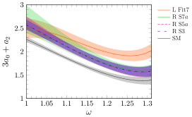
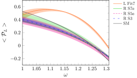
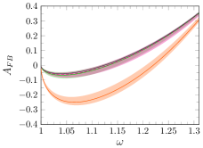
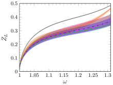
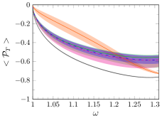
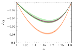
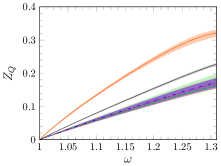
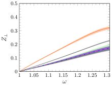
Figure 2: Predictions for the semileptonic observables $(3a_{0}+a_{2}),\langle P^{\rm CM}_{L}\rangle,A_{FB},Z_{L},\langle P^{\rm CM}_{T}\rangle,A_{Q},Z_{Q}$ and $Z_{\perp}$ introduced in Eq. (73), as a function of $\omega$, for the $\Lambda_{b}\to\Lambda_{c}\tau\bar{\nu}_{\tau}$ semileptonic decay. We show results obtained within the SM, the NP model Fit 7 of Ref. Murgui:2019czp , which involves only left-handed neutrinos, and other three ones taken from Ref. Mandal:2020htr , where all included NP operators use right-handed neutrino fields. Error bands account for uncertainties induced by both form-factors and fitted Wilson coefficients (added in quadrature). The right-handed neutrino scenario 3 and the SM lead to the same results for the $A_{FB}(q^{2})$ and $A_{Q}(q^{2})$ angular asymmetries.

In Fig. 2, we show predictions for $(3a_{0}+a_{2}),\langle P^{\rm CM}_{L}\rangle,A_{FB},Z_{L},\langle P^{\rm CM}_{T}\rangle,A_{Q},Z_{Q}$ and $Z_{\perp}$ defined in Eq. (73), for the SM, the NP model Fit 7 of Ref. Murgui:2019czp and for scenarios 3, 5a and 7a from Ref. Mandal:2020htr , which incorporate NP operators constructed using right-handed neutrino fields. All these quantities can be obtained from the $S,P$- and $D$- wave contributions ($F^{d}_{0,1,2}(\omega,\xi_{d})$) to the $d^{3}\Gamma_{d}/(d\omega d\xi_{d}d\cos\theta_{d})$ differential distribution, associated to any of the $\Lambda_{b}\to\Lambda_{c}\tau(\pi\nu_{\tau},\rho\nu_{\tau},\mu\bar{\nu}_{\mu}\nu_{\tau})\bar{\nu}_{\tau}$ sequential decays studied in the previous section. As already stressed, in the absence of CP-violation, this set of observables provides the maximal information (scalar functions ${\cal A},{\cal B},{\cal C}$, and ${\cal A_{H}},{\cal B_{H}},{\cal C_{H}},{\cal D_{H}},{\cal E_{H}}$ in Eqs. (14) and (15)) which can be extracted from the analysis of the semileptonic $\Lambda_{b}\to\Lambda_{c}\tau\bar{\nu}_{\tau}$ transition, considering the most general polarized state for the final tau (see Table 1).

The $(3a_{0}+a_{2})\,\propto\,d\Gamma_{\rm SL}/d\omega$ distributions displayed in the first panel of the figure lead to the results for the integrated widths compiled in Table 2, and it cannot disentangle among the three right-handed neutrino scenarios examined in this work. However, these distributions are useful to efficiently separate between the SM and any of its extensions fitted to the violations of LFU observed in $B$-meson decays. Moreover, for relatively large values of $\omega>1.15$, neutrino left-handed and right-handed NP models predict significantly different $d\Gamma_{\rm SL}/d\omega$ differential decay widths.

In the other seven panels of Fig. 2, we show tau angular and polarization asymmetries, as a function of $\omega$. Relative errors in these observables are smaller than for $(3a_{0}+a_{2})$, since they are defined as ratios for which the form-factor uncertainties largely cancel out. None of these observables are useful in distinguishing between the three scenarios with right-handed neutrinos taken from Ref. Mandal:2020htr . Furthermore, the angular asymmetries $A_{FB}(q^{2})$ and $A_{Q}(q^{2})$, and to some extent the longitudinal polarization average $\langle P^{\rm CM}_{L}\rangle$, do not distinguish between SM and these latter NP models either. The predictions from Fit 7 of Ref. Murgui:2019czp are significantly different from those obtained within the SM and the right-handed neutrino models in all cases, except for $Z_{L}$, where all the extensions of the SM give similar results. The $D$-wave polarization asymmetries $Z_{Q}$ and $Z_{\perp}$ seem quite adequate to distinguish the left-handed Fit 7 and the right-handed neutrino models, since the first type of NP extension produces an increase in the prediction of the SM, while the latter NP scenarios reduce the results of the SM.

5 Summary

We have given the hadron and lepton tensors and the semileptonic differential distributions in the presence of both left- and right-handed neutrino NP terms, and the most general polarization state for the final tau. The formalism is valid for any quark $q\to q\,^{\prime}\ell\bar{\nu}_{\ell}$ or antiquark $\bar{q}\to\bar{q}\,^{\prime}\bar{\ell}\nu_{\ell}$ charged-current decay, although we have usually referred to $b\to c$ transitions. This framework is an alternative to the helicity amplitude one to describe processes where all hadron polarizations are summed up and/or averaged. The results of the first part of this work complete the scheme presented in Ref. Penalva:2020xup , where only left-handed neutrino fields were considered.

In section 3.3, we have discussed the $d^{3}\Gamma_{d}/(d\omega d\cos\theta_{\tau}d\cos\theta_{d}^{*}d\phi_{d}^{*})$ sequential decay distribution in the $\tau$ rest frame, and how it can be used to extract the LAB or CM two dimensional $P_{L}(\omega,\cos\theta_{\tau})$, $P_{T}(\omega,\cos\theta_{\tau})$ and $P_{TT}(\omega,\cos\theta_{\tau})$ components of the $\tau$-polarization vector. These observables, together with the unpolarized $d^{2}\Gamma/(d\omega d\cos\theta_{\tau})$ distribution, provide the maximum information from the $H_{b}\to H_{c}$ semileptonic decay with polarized taus Penalva:2021gef , including the CP-violating contributions driven by the ${\cal F_{H}}$ and ${\cal G_{H}}$ scalar functions (Eqs. (14) and (15)). These latter functions are non zero only when some of the Wilson coefficients are complex, and are extracted from $P_{TT}(\omega,\cos\theta_{\tau})$, the polarization vector component transverse to the plane formed by the outgoing hadron and tau. We have detailed how $P_{TT}$ could be obtained integrating over $\cos\theta_{d}^{*}$, and looking at the $\phi_{d}^{*}$ asymmetry defined in Eq. (48). Results for the CP-violating contributions in the baryon $\Lambda_{b}\to\Lambda_{c}\tau\bar{\nu}_{\tau}$ reaction are shown in Fig. 1 within the $R_{2}$ leptoquark model of Ref. Shi:2019gxi , for which the two nonzero Wilson coefficients ($C^{S}_{LL}$ and $C^{T}_{LL}$) are complex. If the tau momentum is not determined, the $\tau$ rest frame cannot be defined and the former results cannot be experimentally accessed.

Reconstructing the $\tau$ momentum in the final state poses an experimental challenge, because the $\tau$ does not travel far enough for a displaced vertex and its decay involves at least one more invisible neutrino. Direct $\tau$ polarization measurements are even more complicated to perform. Therefore, the maximal accessible information on the $b\to c\tau\bar{\nu}_{\tau}$ transition is encoded in the visible decay products of the $\tau$ lepton. For that reason, we have studied the sequential $H_{b}\to H_{c}\tau\,(\pi\nu_{\tau},\rho\nu_{\tau},\mu\bar{\nu}_{\mu}\nu_{\tau})\bar{\nu}_{\tau}$ decays.

Without relying on the reconstruction of the tau momentum, we have derived the so-called visible decay particle $\pi,\rho,\mu$, distributions Alonso:2016gym ; Alonso:2017ktd ; Asadi:2020fdo , valid for any $H_{b}\to H_{c}$ semileptonic decay. We take as visible kinematical variables the energy $E_{d}$ (or the variable $\xi_{d}$, which is proportional to the energy) of the charged particle in the $\tau$ decay and the angle $\theta_{d}$ made by its three-momentum with that of the final hadron $H_{c}$, both variables defined in the CM frame ($W$ boson at rest). The scheme allows to account for the full set of dimension-6 semileptonic $b\to c$ operators with left- and right-handed neutrinos considered in Ref. Mandal:2020htr .

In the absence of CP-violation, the analysis of the dependence on ($\omega,\xi_{d}$) of the $S,P$- and $D$-wave contributions ($F^{d}_{0,1,2}(\omega,\xi_{d}),\,d=\pi\nu_{\tau},\rho\nu_{\tau},\mu\bar{\nu}_{\mu}\nu_{\tau}$) to the $d^{3}\Gamma_{d}/(d\omega d\xi_{d}d\cos\theta_{d})$ differential distribution provides the maximal information, which can be extracted from the analysis of the semileptonic $H_{b}\to H_{c}\tau\bar{\nu}_{\tau}$ transition, considering the most general polarized state for the final tau. This exhaustive information (scalar functions ${\cal A},{\cal B},{\cal C}$, and ${\cal A_{H}},{\cal B_{H}},{\cal C_{H}},{\cal D_{H}},{\cal E_{H}}$ in Eqs. (14) and (15)) can be rewritten in terms of the overall unpolarized normalization distribution $d\Gamma_{\rm SL}/d\omega$, and seven angular and spin asymmetries [ see Table 1 and Eq. (73)] introduced in Ref. Asadi:2020fdo for $B$-meson decays. We have found that, in general, the hadronic tau-decay channels, and in particular the pion mode, are more convenient to determine the $H_{b}\to H_{c}\tau\bar{\nu}_{\tau}$ semileptonic observables than the lepton $\tau\to\mu\bar{\nu}_{\mu}\nu_{\tau}$ channel. For this latter mode, we have provided, for the very first time, expressions where the muon mass is not set to zero.

We have considered three different extensions of the SM, taken from the recent study in Ref. Mandal:2020htr , that include right-handed neutrino fields, and we have shown predictions (Fig. 2) for the semileptonic observables defined in Eq. (73), for the $\Lambda_{b}\to\Lambda_{c}$ decay. We have compared these NP results with those obtained in the SM, and within an extension of the SM determined by Fit 7 of Ref. Murgui:2019czp constructed with left-handed neutrino operators alone.

None of the semileptonic decay asymmetries turned out to be useful in distinguishing between the three scenarios with right-handed neutrinos. The predictions from Fit 7 of Ref. Murgui:2019czp are, however, significantly different from those obtained within the SM and the right-handed neutrino models in all cases, except for $Z_{L}$, where all the extensions of the SM give similar results. The $D$-wave polarization asymmetries $Z_{Q}$ and $Z_{\perp}$ seem quite adequate to distinguish the left-handed Fit 7 and the right-handed neutrino models.

We are aware that the measurement of these observables is rather difficult. At present, $\Lambda_{b}$’s are only produced at the LHC, where the corresponding $\tau$ decay modes are difficult to reconstruct. However the LHCb collaboration has already published semileptonic decay results where the $\tau$ has been reconstructed through the $\tau\to\mu\nu_{\tau}\bar{\nu}_{\mu}$ decay mode Aaij:2015yra ; Aaij:2017tyk . It is reasonable to expect and extension of this selection strategy to $\Lambda_{b}$ semileptonic decays. The other two $\tau$ decay modes, $\pi\nu_{\tau}$ and $\rho\nu_{\tau}$, analyzed in this work have a lower reconstruction efficiency and are not being exploited at the moment.

Appendix A Wilson coefficients $C_{\chi=L,R}^{S,P,V,A,T}$

We compile in this appendix the coefficients that enter into the definition of the hadron operators in Eq. (12). For left-handed neutrinos ($\chi=L$), we have

$$C^{V}_{L} = (1+C^{V}_{LL}+C^{V}_{RL}),\quad C^{A}_{L}=(1+C^{V}_{LL}-C^{V}_{RL}),$$

$$C^{S}_{L} = (C^{S}_{LL}+C^{S}_{RL}),\quad C^{P}_{L}=(C^{S}_{LL}-C^{S}_{RL}),\quad C^{T}_{L}=C^{T}_{LL},$$ (75)

while for right-handed neutrinos ($\chi=R$),

$$C^{V}_{R} = (C^{V}_{LR}+C^{V}_{RR}),\quad C^{A}_{R}=-(C^{V}_{LR}-C^{V}_{RR}),\quad C^{S}_{R}=(C^{S}_{LR}+C^{S}_{RR}),$$

$$C^{P}_{R} = -(C^{S}_{LR}-C^{S}_{RR}),\quad C^{T}_{R}=C^{T}_{RR},$$ (76)

where $C^{X}_{AB}$ ($X=S,V,T$ and $A,B=L,R$) appear in the BSM effective Hamiltonian of Eq. (1), taken from Ref. Mandal:2020htr .

Appendix B Lepton tensors

From Eq. (8), in the limit of massless neutrinos, we obtain ($h_{\chi}=\pm 1,h=\pm 1$)

$$J^{L}_{(\alpha\beta)}(k,k^{\prime};h,h_{\chi})[J^{L}_{(\rho\lambda)}(k,k^{\prime};h,h_{\chi})]^{*}=\frac{1}{2}{\rm Tr}\Big{[}(\not{k}^{\prime}+m_{\ell})\Gamma_{(\alpha\beta)}P_{5}^{h_{\chi}}\not{k}\,\gamma^{0}\Gamma_{(\rho\lambda)}^{\dagger}\gamma^{0}P_{h}\Big{]}.$$ (77)

The different $\Gamma_{(\alpha\beta)}$ and $\Gamma_{(\rho\lambda)}$ operators give rise to the following lepton tensors (we use the convention $\epsilon_{0123}=+1$ and the short-notation $\epsilon_{\alpha k^{\prime}kS}=\epsilon_{\alpha\delta\eta\sigma}k^{\prime\delta}k^{\eta}S^{\sigma}$, etc.)

$$L(k,k^{\prime};h,h_{\chi}) = \frac{1}{2}\left[k\cdot k^{\prime}-m_{\ell}hh_{\chi}(k\cdot S)\right],$$ (78)

$$L_{\alpha}(k,k^{\prime};h,h_{\chi}) = \frac{m_{\ell}}{2}k_{\alpha}-\frac{h\,h_{\chi}}{2}\left(k^{\prime}_{\alpha}\,k\cdot S-S_{\alpha}\,k\cdot k^{\prime}-ih_{\chi}\epsilon_{\alpha k^{\prime}kS}\right),$$ (79)

$$L^{\prime}_{\rho\lambda}(k,k^{\prime};h,h_{\chi}) = L^{\prime}_{\rho\lambda}(k,k^{\prime};h_{\chi})-hh_{\chi}L^{\prime}_{\rho\lambda}(k,m_{\ell}S;h_{\chi}),$$ (80)

$$L_{\alpha\rho}(k,k^{\prime};h,h_{\chi}) = L_{\alpha\rho}(k,k^{\prime};h_{\chi})+hh_{\chi}L_{\alpha\rho}(k,m_{\ell}S;h_{\chi}),$$ (81)

$$L_{\alpha\rho\lambda}(k,k^{\prime};h,h_{\chi}) = \frac{im_{\ell}}{2}\left(g_{\alpha\lambda}k_{\rho}-g_{\alpha\rho}k_{\lambda}-ih_{\chi}\epsilon_{\alpha\rho\lambda k}\right)+\frac{ihh_{\chi}}{2}\Bigg{\{}k^{\prime}_{\alpha}(S_{\rho}k_{\lambda}-S_{\lambda}k_{\rho})$$ (82)

$$+ k_{\alpha}(S_{\rho}k^{\prime}_{\lambda}-S_{\lambda}k^{\prime}_{\rho})+S_{\alpha}(k_{\rho}k^{\prime}_{\lambda}-k_{\lambda}k^{\prime}_{\rho})+(k\cdot k^{\prime})(g_{\alpha\rho}S_{\lambda}-g_{\alpha\lambda}S_{\rho})$$

$$+ (S\cdot k)(g_{\alpha\lambda}k^{\prime}_{\rho}-g_{\alpha\rho}k^{\prime}_{\lambda})+ih_{\chi}\Big{[}(k\cdot k^{\prime})\epsilon_{\alpha\rho\lambda S}+S_{\lambda}\epsilon_{\alpha\rho k^{\prime}k}-S_{\rho}\epsilon_{\alpha\lambda k^{\prime}k}$$

$$+ k_{\alpha}\epsilon_{\rho\lambda Sk^{\prime}}-k^{\prime}_{\alpha}\epsilon_{\rho\lambda kS}\Big{]}\Bigg{\}},$$

$$L_{\alpha\beta\rho\lambda}(k,k^{\prime};h,h_{\chi}) = \frac{1}{2}\,L_{\alpha\beta\rho\lambda}(k,k^{\prime};h_{\chi})-\frac{hh_{\chi}}{2}L_{\alpha\beta\rho\lambda}(k,m_{\ell}S;h_{\chi}),$$ (83)

which correspond to $(\Gamma_{(\alpha\beta)},\Gamma_{(\rho\lambda)})=(1,1),(\gamma_{\alpha},1),(1,\sigma_{\rho\lambda}),(\gamma_{\alpha},\gamma_{\rho})$, $(\gamma_{\alpha},\sigma_{\rho\lambda})$ and $(\sigma_{\alpha\beta},\sigma_{\rho\lambda})$, respectively, and in Eqs. (81), (80) and (83)

$$L_{\alpha\rho}(k,k^{\prime};h_{\chi}) = \frac{1}{2}\left(k^{\prime}_{\alpha}k_{\rho}+k_{\alpha}k^{\prime}_{\rho}-g_{\alpha\rho}k\cdot k^{\prime}-ih_{\chi}\epsilon_{\alpha\rho k^{\prime}k}\right),$$

$$L^{\prime}_{\rho\lambda}(k,k^{\prime};h_{\chi}) = \frac{i}{2}\left(k_{\rho}k^{\prime}_{\lambda}-k_{\lambda}k^{\prime}_{\rho}-ih_{\chi}\epsilon_{\rho\lambda k^{\prime}k}\right),$$

$$L_{\alpha\beta\rho\lambda}(k,k^{\prime};h_{\chi}) = g_{\beta\rho}(k_{\alpha}k^{\prime}_{\lambda}+k_{\lambda}k^{\prime}_{\alpha})-g_{\beta\lambda}(k_{\alpha}k^{\prime}_{\rho}+k_{\rho}k^{\prime}_{\alpha})-g_{\alpha\rho}(k_{\beta}k^{\prime}_{\lambda}+k_{\lambda}k^{\prime}_{\beta})$$ (84)

$$+ g_{\alpha\lambda}(k_{\beta}k^{\prime}_{\rho}+k_{\rho}k^{\prime}_{\beta})+(k\cdot k^{\prime})(g_{\alpha\rho}g_{\beta\lambda}-g_{\alpha\lambda}g_{\beta\rho})$$

$$- ih_{\chi}\left(k^{\prime}_{\alpha}\epsilon_{\beta\lambda\rho k}-k^{\prime}_{\beta}\epsilon_{\alpha\lambda\rho k}+k_{\rho}\epsilon_{\alpha\beta\lambda k^{\prime}}-k_{\lambda}\epsilon_{\alpha\beta\rho k^{\prime}}\right).$$

Appendix C Hadron tensors

We collect here the hadron tensors that should be contracted with the corresponding lepton ones, compiled in the previous appendix, to obtain $\overline{\sum}|{\cal M}|^{2}_{\nu_{\ell\chi}}$, $\chi=L,R$. The tensorial decompositions, for a given set $C_{\chi}^{S,P,V,A,T}$ of NP Wilson coefficients (see Eqs. (75) and (76)), are taken from Ref. Penalva:2020xup .

• The spin-averaged squared of the $O_{H\chi}^{\alpha}$ operator matrix element leads to

  $$W^{\alpha\rho}_{\chi}(p,q,C^{V}_{\chi},C^{A}_{\chi}) = \overline{\sum_{r,r^{\prime}}}\langle H_{c};p^{\prime},r^{\prime}|(C^{V}_{\chi}V^{\alpha}+h_{\chi}C^{A}_{\chi}A^{\alpha})|H_{b};p,r\rangle\times$$ (85)

  $$\times \langle H_{c};p^{\prime},r^{\prime}|(C^{V}_{\chi}V^{\rho}+h_{\chi}C^{A}_{\chi}A^{\rho})|H_{b};p,r\rangle^{*},$$

  with $(C^{V}_{\chi}V^{\alpha}+h_{\chi}C^{A}_{\chi}A^{\alpha})=\bar{c}(0)\gamma^{\alpha}(C^{V}_{\chi}+h_{\chi}C^{A}_{\chi}\gamma_{5})b(0)$. The sum is done over initial (averaged) and final hadron helicities, and the above tensor should be contracted with the lepton one $L_{\alpha\rho}(k,k^{\prime};h,h_{\chi})$ (Eq. (81)) to get the contribution to $\overline{\sum}\,|{\cal M}|^{2}_{\nu_{\ell\chi}}$, $\chi=L,R$. The tensor can be expressed in terms of five SFs as

  $$W^{\alpha\rho}_{\chi}(p,q,C^{V}_{\chi},C^{A}_{\chi}) = -g^{\alpha\rho}\widetilde{W}_{1\chi}+\frac{p^{\alpha}p^{\rho}}{M^{2}}\widetilde{W}_{2\chi}-ih_{\chi}\epsilon^{\alpha\rho\delta\eta}p_{\delta}q_{\eta}\frac{\widetilde{W}_{3\chi}}{2M^{2}}$$ (86)

  $$+ \frac{q^{\alpha}q^{\rho}}{M^{2}}\widetilde{W}_{4\chi}+\dfrac{p^{\alpha}q^{\rho}+p^{\rho}q^{\alpha}}{2M^{2}}\widetilde{W}_{5\chi},$$

  where all $\widetilde{W}_{1\chi,2\chi,3\chi,4\chi,5\chi}(q^{2},C^{V}_{\chi},C^{A}_{\chi})$ SFs are real. Following the notation in Ref. Penalva:2020xup ,

  $$\widetilde{W}_{1\chi,2\chi,4\chi,5\chi}(q^{2}) = |C^{V}_{\chi}|^{2}W_{1,2,4,5}^{VV}(q^{2})+|C^{A}_{\chi}|^{2}W_{1,2,4,5}^{AA}(q^{2}),\,$$

  $$\widetilde{W}_{3\chi}(q^{2}) = {\rm Re}(C^{V}_{\chi}C^{A*}_{\chi})W_{3}^{V\!\!A}(q^{2}).$$ (87)

• The diagonal contribution of the tensor operator $O_{H\chi}^{\alpha\beta}$ gives rise to

  $$W_{\chi}^{\alpha\beta\rho\lambda}(p,q,C^{T}_{\chi}) = |C^{T}_{\chi}|^{2}\overline{\sum_{r,r^{\prime}}}\langle H_{c};p^{\prime},r^{\prime}|\bar{c}(0)\sigma_{\alpha\beta}(1+h_{\chi}\gamma_{5})b(0)|H_{b};p,r\rangle\times$$ (88)

  $$\times \langle H_{c};p^{\prime},r^{\prime}|\bar{c}(0)\sigma_{\rho\lambda}(1+h_{\chi}\gamma_{5})b(0)|H_{b};p,r\rangle^{*},$$

  which contracted with the lepton tensor $L_{\alpha\beta\rho\lambda}(k,k^{\prime};h,h_{\chi})$ in Eq. (83) provides the $L$ or $R$ contributions to the differential decay rate. The total tensor can be expressed in terms of four real SFs,

  $$W^{\alpha\beta\rho\lambda}_{\chi} = |C^{T}_{\chi}|^{2}\Bigg{\{}W_{1}^{T}\Big{[}g^{\alpha\rho}g^{\beta\lambda}-g^{\alpha\lambda}g^{\beta\rho}+ih_{\chi}\epsilon^{\rho\lambda\alpha\beta}\Big{]}+\frac{W_{2}^{T}}{M^{2}}\Big{[}g^{\alpha\rho}p^{\beta}p^{\lambda}-g^{\alpha\lambda}p^{\beta}p^{\rho}$$ (89)

  $$- g^{\beta\rho}p^{\alpha}p^{\lambda}+g^{\beta\lambda}p^{\alpha}p^{\rho}+ih_{\chi}\Big{(}\epsilon^{\rho\lambda\alpha\delta}p^{\beta}p_{\delta}-\epsilon^{\rho\lambda\beta\delta}p^{\alpha}p_{\delta}\Big{)}\Big{]}$$

  $$+ \frac{W_{3}^{T}}{M^{2}}\Big{[}g^{\alpha\rho}q^{\beta}q^{\lambda}-g^{\alpha\lambda}q^{\beta}q^{\rho}-g^{\beta\rho}q^{\alpha}q^{\lambda}+g^{\beta\lambda}q^{\alpha}q^{\rho}$$

  $$+ ih_{\chi}\Big{(}\epsilon^{\rho\lambda\alpha\delta}q^{\beta}q_{\delta}-\epsilon^{\rho\lambda\beta\delta}q^{\alpha}q_{\delta}\Big{)}\Big{]}+\frac{W_{4}^{T}}{M^{2}}\Big{[}g^{\alpha\rho}(p^{\beta}q^{\lambda}+p^{\lambda}q^{\beta})$$

  $$- g^{\alpha\lambda}(p^{\beta}q^{\rho}+p^{\rho}q^{\beta})-g^{\beta\rho}(p^{\alpha}q^{\lambda}+p^{\lambda}q^{\alpha})+g^{\beta\lambda}(p^{\alpha}q^{\rho}+p^{\rho}q^{\alpha})$$

  $$+ ih_{\chi}\Big{(}\epsilon^{\rho\lambda\alpha\delta}(p^{\beta}q_{\delta}+q^{\beta}p_{\delta})-\epsilon^{\rho\lambda\beta\delta}(p^{\alpha}q_{\delta}+q^{\alpha}p_{\delta})\Big{)}\Big{]}\Bigg{\}}.$$

  The $W_{1,2,3,4}^{T}$ SFs are found from $(W^{\alpha\beta\rho\lambda}_{TT}+W^{\alpha\beta\rho\lambda}_{pTpT})$ Penalva:2020xup and accomplish the constraint

  $$2M^{2}W_{1}^{T}+p^{2}W_{2}^{T}+q^{2}W_{3}^{T}+2(p\cdot q)W_{4}^{T}=0,$$ (90)

  which can be used to re-write $W_{1}^{T}$ in terms of $W^{T}_{2,3,4}$. In any case, the contraction of the $W_{1}^{T}$-part of the tensor with $L_{\alpha\beta\rho\lambda}(k,k^{\prime};h,h_{\chi})$ is zero, and thus the contribution of $W^{\alpha\beta\rho\lambda}_{\chi}$ to $\overline{\sum}|{\cal M}|^{2}_{\nu_{\ell\chi}}$ is given only in terms of $W_{2}^{T}$, $W_{3}^{T}$ and $W_{4}^{T}$. The common factor $|C^{T}_{\chi}|^{2}$ was absorbed in Penalva:2020xup by introducing $\widetilde{W}^{T}_{1\chi,2\chi,3\chi,4\chi}=|C^{T}_{\chi}|^{2}W^{T}_{1,2,3,4}$.

• The diagonal contribution of the operator $O_{H\chi}$ leads to the real scalar SF

  $$W_{\chi}(p,q) = \widetilde{W}_{SP\chi}(q^{2})=|C^{S}_{\chi}|^{2}\overline{\sum_{r,r^{\prime}}}|\langle H_{c};p^{\prime},r^{\prime}|\bar{c}(0)b(0)|H_{b};p,r\rangle|^{2}$$ (91)

  $$+ |C^{P}_{\chi}|^{2}\overline{\sum_{r,r^{\prime}}}|\langle H_{c};p^{\prime},r^{\prime}|\bar{c}(0)\gamma_{5}b(0)|H_{b};p,r\rangle|^{2},$$

  which should be multiplied by the scalar lepton term of Eq. (78).

• The $O_{H\chi}^{\alpha}$ and $O_{H\chi}$ interference contribute to $\overline{\sum}\,|{\cal M}|^{2}_{\nu_{\ell\chi}}$ as $2{\rm Re}\Big{[}L_{\alpha}(k,k^{\prime};h,h_{\chi})\times$ $W^{\alpha}_{\chi}(p,q,C^{V,A,S,P}_{\chi})\Big{]}$, with the lepton tensor defined in Eq. (79) and

  $$W^{\alpha}_{\chi}(p,q,C^{V,A,S,P}_{\chi}) = \overline{\sum_{r,r^{\prime}}}\langle H_{c};p^{\prime},r^{\prime}|(C^{V}_{\chi}V^{\alpha}+h_{\chi}C^{A}_{\chi}A^{\alpha})|H_{b};p,r\rangle\times$$ (92)

  $$\times \langle H_{c};p^{\prime},r^{\prime}|\bar{c}(0)(C^{S}_{\chi}+h_{\chi}C^{P}_{\chi}\gamma_{5})b(0)|H_{b};p,r\rangle^{*}$$

  $$= \frac{1}{2M}\left(\widetilde{W}_{I1\chi}p^{\alpha}+\widetilde{W}_{I2\chi}q^{\alpha}\right),$$

  where $\widetilde{W}_{I1\chi,I2\chi}$ are obtained as

  $$\widetilde{W}_{I1\chi,I2\chi}(q^{2})=C^{V}_{\chi}C^{S*}_{\chi}W^{VS}_{I1,I2}(q^{2})+C^{A}_{\chi}C^{P*}_{\chi}W^{AP}_{I1,I2}(q^{2}),$$ (93)

  with all four $W^{VS,AP}_{I1,I2}$ real functions of $q^{2}$ Penalva:2020xup .

• The $O_{H\chi}$ and $O_{H\chi}^{\rho\lambda}$ interference contribute to $\overline{\sum}\,|{\cal M}|^{2}_{\nu_{\ell\chi}}$ as $2{\rm Re}\Big{[}L^{\prime}_{\rho\lambda}(k,k^{\prime};h,h_{\chi})\times$ $W^{\prime\rho\lambda}_{\chi}(p,q,C^{S,P,T}_{\chi})\Big{]}$, with the lepton tensor defined in Eq. (80) and

  $$W_{\chi}^{\prime\rho\lambda}(p,q,C^{S,P,T}_{\chi}) = C^{T*}_{\chi}\overline{\sum_{r,r^{\prime}}}\langle H_{c};p^{\prime},r^{\prime}|\bar{c}(0)(C^{S}_{\chi}+h_{\chi}C^{P}_{\chi}\gamma_{5})b(0)|H_{b};p,r\rangle\times$$ (94)

  $$\times \langle H_{c};p^{\prime},r^{\prime}|\bar{c}(0)\sigma^{\rho\lambda}(1+h_{\chi}\gamma_{5})b(0)|H_{b};p,r\rangle^{*}$$

  $$= \frac{\widetilde{W}_{I3\chi}}{2M^{2}}\left[i(p^{\rho}q^{\lambda}-p^{\lambda}q^{\rho})-h_{\chi}\epsilon^{\rho\lambda\delta\eta}p_{\delta}q_{\eta}\right],$$

  with Penalva:2020xup

  $$\widetilde{W}_{I3\chi}(q^{2})=C^{T^{*}}_{\chi}\left(C^{S}_{\chi}W_{I3}^{ST}(q^{2})+C^{P}_{\chi}W_{I3}^{PpT}(q^{2})\right)$$ (95)

  and $W_{I3}^{ST,PpT}$ real scalar functions of $q^{2}$.

• The $O^{\alpha}_{H\chi}$ and $O_{H\chi}^{\rho\lambda}$ interference contribute to the decay width as $2{\rm Re}\Big{[}L_{\alpha\rho\lambda}(k,k^{\prime};h)\times$ $W^{\alpha\rho\lambda}_{\chi}(p,q,C^{V,A,T}_{\chi})\Big{]}$, with the lepton tensor defined in Eq. (82) and

  $$W^{\alpha\rho\lambda}_{\chi}(p,q,C^{V,A,T}_{\chi}) = C^{T*}_{\chi}\overline{\sum_{r,r^{\prime}}}\langle H_{c};p^{\prime},r^{\prime}|(C^{V}_{\chi}V^{\alpha}+h_{\chi}C^{A}_{\chi}A^{\alpha})|H_{b};p,r\rangle\times$$ (96)

  $$\times \langle H_{c};p^{\prime},r^{\prime}|\bar{c}(0)\sigma^{\rho\lambda}(1+h_{\chi}\gamma_{5})b(0)|H_{b};p,r\rangle^{*}$$

  $$= \frac{p^{\alpha}\widetilde{W}_{I4\chi}+q^{\alpha}\widetilde{W}_{I5\chi}}{2M^{3}}\left[i(p^{\rho}q^{\lambda}-p^{\lambda}q^{\rho})-h_{\chi}\epsilon^{\rho\lambda\delta\eta}p_{\delta}q_{\eta}\right]$$

  $$+ \frac{p_{\delta}\widetilde{W}_{I6\chi}+q_{\delta}\widetilde{W}_{I7\chi}}{2M}\left[i(g^{\alpha\rho}g^{\lambda\delta}-g^{\alpha\lambda}g^{\rho\delta})-h_{\chi}\epsilon^{\rho\lambda\alpha\delta}\right],$$

  where the SFs are obtained from Penalva:2020xup

  $$\widetilde{W}_{I4\chi,I5\chi,I6\chi,I7\chi}(q^{2})=C^{T*}_{\chi}\left(C^{V}_{\chi}W_{I4,I5,I6,I7}^{VT}(q^{2})+C^{A}_{\chi}W_{I4,I5,I6,I7}^{ApT}(q^{2})\right),$$ (97)

  with $W_{I4,I5,I6,I7}^{VT}$ and $W_{I4,I5,I6,I7}^{ApT}$ real scalar functions of $q^{2}$, which are given in terms of the form-factors used to parameterize the hadronic matrix elements.

Appendix D $\left(|{\cal M}|_{\nu_{\ell L}}^{2}+|{\cal M}|_{\nu_{\ell R}}^{2}\right)$ in terms of the $\widetilde{W}$ SFs

In this appendix we collect the expressions of the ${\cal A},{\cal B}$ and ${\cal C}$ and ${\cal A}_{H},{\cal B}_{H}$, ${\cal C}_{H},{\cal D}_{H},{\cal E}_{H},{\cal F}_{H}$ and ${\cal G}_{H}$ functions introduced in Eq. (14), and that describe, respectively, the semileptonic decay for the cases of unpolarized and polarized outgoing charged leptons. They are combinations of the hadronic $\widetilde{W}$ SFs and receive contributions from both neutrino chiralities (symbolically $\widetilde{W}_{\chi}=C_{\chi}W$) . For ${\cal A},{\cal B},{\cal C}$ and the CP-violating ${\cal F}_{H}$ and ${\cal G}_{H}$, it always appears the combination $(L+R)$, i.e. $(\widetilde{W}_{iL}+\widetilde{W}_{iR})$, while for ${\cal A_{H}},{\cal B_{H}},{\cal C_{H}},{\cal D_{H}}$ and ${\cal E_{H}}$ the structure is ($L-R):$ ($\widetilde{W}_{iL}-\widetilde{W}_{iR})$. The explicit expressions, for any semileptonic decay driven by a $q\to q^{\prime}\ell\bar{\nu}_{\ell}$ transition, read ($M_{\omega}=M-M^{\prime}\omega$)

$${\cal A}(\omega) = \frac{q^{2}-m_{\ell}^{2}}{M^{2}}\sum_{\chi=L,R}\Bigg{\{}2\widetilde{W}_{1\chi}-\widetilde{W}_{2\chi}+\frac{M_{\omega}}{M}\widetilde{W}_{3\chi}+\widetilde{W}_{SP\chi}+8\widetilde{W}_{2\chi}^{T}-\frac{8q^{2}}{M^{2}}\widetilde{W}_{3\chi}^{T}$$

$$- \frac{16M_{\omega}}{M}\widetilde{W}_{4\chi}^{T}+\frac{m_{\ell}}{M}{\rm Re}\left[\widetilde{W}_{I2\chi}+4\,\widetilde{W}_{I4\chi}+\frac{4M_{\omega}}{M}\widetilde{W}_{I5\chi}+12\,\widetilde{W}_{I7\chi}\right]$$

$$+ \frac{4M_{\omega}}{M}{\rm Re}[\widetilde{W}_{I3\chi}]+\frac{m_{\ell}^{2}}{M^{2}}\left(\widetilde{W}_{4\chi}-16\widetilde{W}_{3\chi}^{T}\right)\Bigg{\}},$$

$${\cal B}(\omega) = \sum_{\chi=L,R}\Bigg{\{}-\frac{2q^{2}}{M^{2}}\left(\widetilde{W}_{3\chi}+4{\rm Re}[\widetilde{W}_{I3\chi}]\right)+\frac{4M_{\omega}}{M}\Big{(}\widetilde{W}_{2\chi}-16\,\widetilde{W}_{2\chi}^{T}\Big{)}$$

$$+ \frac{2m_{\ell}}{M}{\rm Re}\left[\widetilde{W}_{I1\chi}-\frac{4M_{\omega}}{M}\widetilde{W}_{I4\chi}-\frac{4q^{2}}{M^{2}}\widetilde{W}_{I5\chi}+12\,\widetilde{W}_{I6\chi}\right]$$

$$+ \frac{2m_{\ell}^{2}}{M^{2}}\left(\widetilde{W}_{5\chi}-32\,\widetilde{W}_{4\chi}^{T}\right)\Bigg{\}},$$

$${\cal C}(\omega) = -4\sum_{\chi=L,R}\Big{(}\widetilde{W}_{2\chi}-16\,\widetilde{W}_{2\chi}^{T}\Big{)},$$ (98)

$${\cal A_{H}}(\omega) = \frac{q^{2}-m^{2}_{\ell}}{2M^{2}}\sum_{\chi=L,R}h_{\chi}\Bigg{\{}{\rm Re}\left[\widetilde{W}_{I1\chi}+\frac{4M_{\omega}}{M}\widetilde{W}_{I4\chi}-4\,\widetilde{W}_{I6\chi}\right]$$

$$+ \frac{m_{\ell}}{M}\left(\widetilde{W}_{3\chi}+\widetilde{W}_{5\chi}-4\,{\rm Re}[\widetilde{W}_{I3\chi}]+32\,\widetilde{W}_{4\chi}^{T}\right)-\frac{4m_{\ell}^{2}}{M^{2}}{\rm Re}[\widetilde{W}_{I5\chi}]\Bigg{\}},$$

$${\cal B_{H}}(\omega) = -\sum_{\chi=L,R}h_{\chi}\Bigg{\{}\frac{M_{\omega}}{M}{\rm Re}\left[\widetilde{W}_{I1\chi}+\frac{4M_{\omega}}{M}\widetilde{W}_{I4\chi}-4\,\widetilde{W}_{I6\chi}\right]-\frac{m_{\ell}}{M}\left(2\,\widetilde{W}_{1\chi}\right.$$

$$- \left.\widetilde{W}_{2\chi}-\frac{M_{\omega}}{M}\widetilde{W}_{5\chi}-\widetilde{W}_{SP\chi}-8\,\widetilde{W}_{2\chi}^{T}+\frac{8q^{2}}{M^{2}}\widetilde{W}_{3\chi}^{T}-\frac{16M_{\omega}}{M}\widetilde{W}_{4\chi}^{T}\right)$$

$$+ \frac{m_{\ell}^{2}}{M^{2}}{\rm Re}\left[\widetilde{W}_{I2\chi}-4\,\widetilde{W}_{I4\chi}-4\,\widetilde{W}_{I7\chi}\right]+\frac{m_{\ell}^{3}}{M^{3}}\left(\widetilde{W}_{4\chi}+16\,\widetilde{W}_{3\chi}^{T}\right)\Bigg{\}},$$

$${\cal C_{H}}(\omega) = -\sum_{\chi=L,R}h_{\chi}\Bigg{\{}\frac{4q^{2}}{M^{2}}{\rm Re}[\widetilde{W}_{I4\chi}]-\frac{2m_{\ell}}{M}\left(\widetilde{W}_{2\chi}+16\widetilde{W}_{2\chi}^{T}\right)+\frac{4m_{\ell}^{2}}{M^{2}}{\rm Re}[\widetilde{W}_{I4\chi}]\Bigg{\}},$$

$${\cal D_{H}}(\omega) = \sum_{\chi=L,R}h_{\chi}\Bigg{\{}{\rm Re}\left[\widetilde{W}_{I1\chi}+\frac{12M_{\omega}}{M}\widetilde{W}_{I4\chi}-4\,\widetilde{W}_{I6\chi}\right]$$

$$-\frac{m_{\ell}}{M}\left(\widetilde{W}_{3\chi}-\widetilde{W}_{5\chi}-32\widetilde{W}_{4\chi}^{T}-4{\rm Re}[\widetilde{W}_{I3\chi}]\right)+\frac{4m^{2}_{\ell}}{M^{2}}{\rm Re}[\widetilde{W}_{I5\chi}]\Bigg{\}},$$

$${\cal E_{H}}(\omega) = -8\,\sum_{\chi=L,R}h_{\chi}{\rm Re}[\widetilde{W}_{I4\chi}],$$ (99)

$${\cal F_{H}}(\omega) = 4\sum_{\chi=L,R}{\rm Im}\bigg{[}\frac{\widetilde{W}_{I1\chi}}{4}+\frac{m_{\ell}}{M}\widetilde{W}_{I3\chi}+\frac{M_{\omega}}{M}\widetilde{W}_{I4\chi}+\frac{m^{2}_{\ell}}{M^{2}}\widetilde{W}_{I5\chi}-\widetilde{W}_{I6\chi}\bigg{]},$$

$${\cal G_{H}}(\omega) = -8\sum_{\chi=L,R}{\rm Im}[\widetilde{W}_{I4\chi}].$$ (100)

with $h_{\chi=R}=1$ and $h_{\chi=L}=-1$. Finally, expressions for the $\widetilde{W}_{i\chi}$ SFs in terms of the Wilson coefficients and the form-factors, used to parameterize the genuine hadronic responses $W_{i}$, can be obtained from the Appendices E of Ref. Penalva:2020xup and B of Penalva:2020ftd for the $\Lambda_{b}^{0}\to\Lambda_{c}^{+}\ell^{-}\bar{\nu}_{\ell}$ and $P_{b}\to P_{c}^{(*)}\ell^{-}\bar{\nu}_{\ell}$ decays, respectively. In fact, replacing

$$C_{V,A,S,P,T}\to C^{V,A,S,P,T}_{\chi}$$ (101)

in these last works, all $\widetilde{W}_{i\chi}$ SFs are obtained. Furthermore, using the appropriate form-factors, the results of Refs. Penalva:2020xup and Penalva:2020ftd can be used to describe any $1/2^{+}\to 1/2^{+}$, $0^{-}\to 0^{-}$ or $0^{-}\to 1^{-}$ semileptonic decay, regardless of the involved flavors (see also the last comment in Appendix E).

Appendix E Antiquark-driven semileptonic decays

The hermitian conjugate terms of the effective Hamiltonian of Eq. (1), not explicitly written in that equation, can be used to evaluate the semileptonic decay

$$H_{\bar{b}}\to H_{\bar{c}}\ell^{+}\nu_{\ell}$$ (102)

driven by the antiquark $\bar{b}\to\bar{c}\ell^{+}\nu_{\ell}$ transition, and obviously this reaction can be related to that involving $b$ and $c$ quarks. Looking at the ${\cal M}|_{\ell\bar{\nu}_{\ell}}$ and ${\cal M}|_{\bar{\ell}\nu_{\ell}}$ amplitudes, and using charge-conjugation transformations of the hadron operators and states Itzykson:1980rh we first find,

$$\langle H_{\bar{c}};p^{\prime},r^{\prime}|\bar{b}~{}\widetilde{O}_{H\chi}^{(\alpha\beta)}c|H_{\bar{b}};p,r\rangle=\langle H_{c};p^{\prime},r^{\prime}|\bar{c}~{}O_{H\chi}^{(\alpha\beta)}b|H_{b};p,r\rangle\Bigg{|}_{\begin{array}[]{c}C_{\chi}^{V,A,T}\to-\left(C_{\chi}^{V,A,T}\right)^{*}\\ C_{\chi}^{S,P}\to\left(C_{\chi}^{S,P}\right)^{*}\\ h_{\chi}\to-h_{\chi}\end{array}},$$ (103)

with $\widetilde{O}_{H\chi}=\gamma^{0}O_{H\chi}^{\dagger}\gamma^{0}$. For the leptonic part of the amplitude, we use now the properties of the charge conjugation matrix in the Dirac space and its action on Dirac spinors and matrices Itzykson:1980rh to get

$$J^{L;\bar{\ell}\nu_{\ell}}_{(\alpha\beta)}(k,k^{\prime};h,h_{\chi}) = \frac{1}{\sqrt{2}}\bar{u}_{\nu_{\ell}}(k)P_{5}^{-h_{\chi}}\gamma^{0}\Gamma_{(\alpha\beta)}^{\dagger}\gamma^{0}v_{\ell}^{S}(k^{\prime};h)$$ (104)

$$= (-1)^{n_{L}+1}\frac{1}{\sqrt{2}}\bar{u}_{\ell}^{S}(k^{\prime};h)P_{h}\Gamma_{(\alpha\beta)}P_{5}^{-h_{\chi}}v_{\nu_{\ell}}(k)$$

$$= (-1)^{n_{L}+1}J^{L;\ell\bar{\nu}_{\ell}}_{(\alpha\beta)}(k,k^{\prime};h,-h_{\chi}),$$

with $n_{L}=1$ for $\Gamma_{(\alpha\beta)}=(\gamma_{\alpha},\sigma_{\alpha\beta})$ and $n_{L}=0$ for $\Gamma_{(\alpha\beta)}=1$. The factor $(-1)^{n_{L}}$ compensates the relative sign between $C_{\chi}^{S,P}$ and $C_{\chi}^{V,A,T}$ in Eq. (103), while the extra minus sign in Eq. (104) is of no consequence in evaluating the amplitude squared. Taking the complex-conjugate of the Wilson coefficients has no effects when calculating their squared moduli or the real part of the product of two of them, but it does produce a minus sign when the imaginary part of the product of two of them is considered instead. All together, from Eqs. (103)–(104) and (98)–(100), we conclude that ${\cal A},{\cal B}$ and ${\cal C}$ are identical for both quark and antiquark decays, while the ${\cal A_{H}},{\cal B_{H}},{\cal C_{H}},{\cal D_{H}}$, ${\cal E_{H}}$, ${\cal F_{H}}$ and ${\cal G_{H}}$ antiquark functions get a global sign. The first five because they are proportional to $h_{\chi}$, while in the case of ${\cal F_{H}}$ and ${\cal G_{H}}$, they are proportional to the imaginary part of the product of two Wilson coefficients. Hence, we obtain

$$\frac{2\,\overline{\sum}\,|{\cal M}|^{2}}{M^{2}}\Big{|}_{H_{\bar{b}}\to H_{\bar{c}}} = {\cal N}(\omega,p\cdot k)-h\bigg{\{}\frac{(p\cdot S)}{M}\,{\cal N_{H_{\rm 1}}}(\omega,p\cdot k)$$ (105)

$$+ \frac{(q\cdot S)}{M}\,{\cal N_{H_{\rm 2}}}(\omega,p\cdot k)+\frac{\epsilon^{Sk^{\prime}qp}}{M^{3}}\,{\cal N_{H_{\rm 3}}}(\omega,p\cdot k)\ \bigg{\}},$$

with the ${\cal N}$ and $\cal N_{H_{\rm 123}}$ scalar functions identical to those that appear in the $H_{b}\to H_{c}$ decay, and the charged-lepton produced in the polarized state $v_{\ell}^{S}(k^{\prime};h)$ that satisfies

$$\gamma_{5}\not{S}\,v_{\ell}^{S}(k^{\prime};h)=h\,v_{\ell}^{S}(k^{\prime};h).$$ (106)

Note also that Eq. (104) and the results for $\widetilde{W}$ SFs compiled in Appendix C, for NP operators involving both left- and right-handed neutrino fields, can be straightforwardly used to describe quark charged-current transitions giving rise to a final $\ell^{+}\nu_{\ell}$ lepton pair (e.g. $c\to s\ell^{+}\nu_{\ell}$). From Eq. (104) it is clear that left/right leptonic currents for $\bar{\ell}\nu_{\ell}$ production are related to right/left leptonic currents for $\ell\bar{\nu}_{\ell}$ production.

Appendix F Phase space integrations

Here we give several results and formulae used in the integration of the available phase space in the sequential $H_{b}\to H_{c}\tau\,(\pi\nu_{\tau},\rho\nu_{\tau},\mu\bar{\nu}_{\mu}\nu_{\tau})\bar{\nu}_{\tau}$ decays.

First, we note

$$\frac{\delta^{4}\left(q-k-\tilde{p}_{d}\right)}{\left[(q-k)^{2}-m^{2}_{\tau}\right]^{2}+(q-k)^{2}\Gamma^{2}_{\tau}\left[(q-k)^{2}\right]} = \int d^{4}k^{\prime}\delta^{4}(k^{\prime}-(q-k))\times$$ (107)

$$\times \int dz^{2}\frac{\delta(z^{2}-k^{\prime\,2})\delta^{4}(k^{\prime}-\tilde{p}_{d})}{\left(z^{2}-m^{2}_{\tau}\right)^{2}+z^{2}\Gamma^{2}_{\tau}(z^{2})},$$

with $\tilde{p}_{d}$ the total four-momentum of all decay products of the virtual $\tau$ (e.g. $\tilde{p}_{d}=p_{\pi}+p_{\nu_{\tau}}$ for the pion mode). Now using $\delta(z^{2}-k^{\prime\,2})=\delta\big{[}k^{\prime\,0}-\sqrt{z^{2}+\vec{k}^{\prime\,2}}\,\big{]}/(2k^{\prime\,0})$, since $k^{\prime\,0}=\tilde{p}_{d}^{0}>0$,

$$\frac{\delta^{4}\left(q-k-\tilde{p}_{d}\right)}{\left[\tilde{p}_{d}^{2}-m^{2}_{\tau}\right]^{2}+\tilde{p}_{d}^{2}\Gamma^{2}_{\tau}\left[\tilde{p}_{d}^{2}\right]} = \int\frac{dz^{2}}{\left(z^{2}-m^{2}_{\tau}\right)^{2}+z^{2}\Gamma^{2}_{\tau}(z^{2})}\times$$ (108)

$$\times \int\frac{d^{3}k^{\prime}}{2\sqrt{z^{2}+\vec{k}^{\prime\,2}}}\delta^{4}(q-k^{\prime}-k)\delta^{4}(k^{\prime}-\tilde{p}_{d}),$$

with $k^{\prime\,0}=\sqrt{z^{2}+\vec{k}^{\prime\,2}}$. Finally, the narrow width approximation of Eq. (36) leads to

$$\frac{\delta^{4}\left(q-k-\tilde{p}_{d}\right)}{\left[\tilde{p}_{d}^{2}-m^{2}_{\tau}\right]^{2}+\tilde{p}_{d}^{2}\Gamma^{2}_{\tau}\left[\tilde{p}_{d}^{2}\right]} \simeq \frac{\pi}{m_{\tau}\Gamma_{\tau}}\int\frac{d^{3}k^{\prime}}{2\sqrt{m_{\tau}^{2}+\vec{k}^{\prime\,2}}}\delta^{4}(q-k^{\prime}-k)\delta^{4}(k^{\prime}-\tilde{p}_{d}),$$ (109)

with the $\tau$ on the mass shell.

In the second place, we find for the $(\nu_{\tau},\bar{\nu}_{\mu})$ phase-space integration of the muon polarization sum ${\cal R}_{\mu\bar{\nu}_{\mu}}$ (Eq. (33))

$$\int\frac{d^{3}p_{\nu_{\tau}}}{2|\vec{p}_{\nu_{\tau}}|}\int\frac{d^{3}p_{\bar{\nu}_{\mu}}}{2|\vec{p}_{\bar{\nu}_{\mu}}|}\delta^{4}(Q-p_{\nu_{\tau}}-p_{\bar{\nu}_{\mu}}){\cal R}_{\mu\bar{\nu}_{\mu}} = \frac{\pi m_{\tau}^{3}}{3}H(1+y^{2}-x)\Big{[}G_{1}(x,y)$$ (110)

$$+ \frac{2(p_{\mu}{\cal P})}{m_{\tau}}\left(1+3y^{2}-2x\right)\Big{]}.$$

with $Q=k^{\prime}-p_{\mu}$, $x=2(p_{\mu}\cdot k^{\prime})/m^{2}_{\tau}$, $y^{2}=m^{2}_{\mu}/m^{2}_{\tau}$, $G_{1}(x,y)=x(3-2x)-y^{2}(4-3x)$ and $H[...]$ the step function. This result is obtained by using that for massless neutrinos

$$\int\frac{d^{3}p_{\nu_{\tau}}}{2|\vec{p}_{\nu_{\tau}}|}\int\frac{d^{3}p_{\bar{\nu}_{\mu}}}{2|\vec{p}_{\bar{\nu}_{\mu}}|}\delta^{4}(Q-p_{\nu_{\tau}}-p_{\bar{\nu}_{\mu}})p_{\nu_{\tau}}^{\alpha}p_{\bar{\nu}_{\mu}}^{\beta}=\frac{\pi Q^{2}}{24}\left(g^{\alpha\beta}+2\frac{Q^{\alpha}Q^{\beta}}{Q^{2}}\right)H[Q^{2}].$$ (111)

Finally, in section 3.4, and in order to perform the $\cos\theta_{\tau}$ integrations in the CM frame, we make use of

$$\frac{1}{\pi}\int_{a}^{b}d\alpha\frac{t_{0}+t_{1}\alpha+t_{2}\alpha^{2}}{\sqrt{(b-\alpha)(\alpha-a)}}=t_{0}+\frac{t_{2}}{3}+t_{1}\cos\theta_{\tau d}^{\rm CM}\cos\theta_{d}+\frac{2t_{2}}{3}P_{2}(\cos\theta_{\tau d}^{\rm CM})P_{2}(\cos\theta_{d}),$$ (112)

with $a=\cos(\theta_{d}+\theta_{\tau d}^{\rm CM})$, $b=\cos(\theta_{d}-\theta_{\tau d}^{\rm CM})$ and $P_{2}$ the Legendre polynomial of order 2.

Appendix G $C_{n},C_{P_{L}},C_{A_{FB}},C_{Z_{L}},C_{P_{T}},C_{A_{Q}},C_{Z_{Q}}$ and $C_{Z_{\perp}}$ coefficients and their dependence on $(\omega,\xi_{d})$

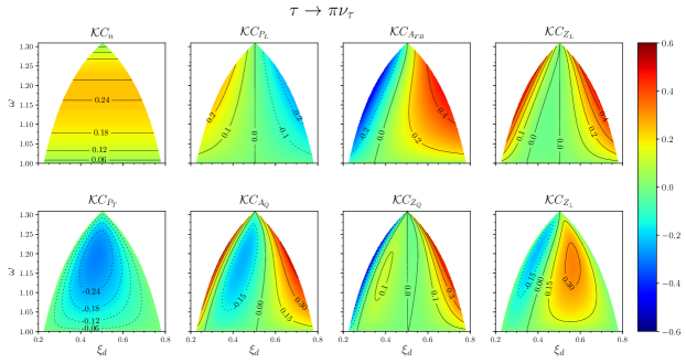
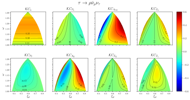
Figure 3: Two dimensional $(\omega,\xi_{d})$ dependence of the coefficients [multiplied by the kinematical factor ${\cal K}(\omega)=\sqrt{\omega^{2}-1}\,(1-m_{\tau}^{2}/q^{2})^{2}$ ] introduced in Eq. (74) for the $\pi$ and $\rho$ hadronic tau-decay modes. Each of the coefficients affects one of the observables introduced in Eq. (73), within the corresponding $F^{d}_{0,1,2}(\omega,\xi_{d})$ partial wave contribution to the $d^{3}\Gamma_{d}/(d\omega d\xi_{d}d\cos\theta_{d})$ differential decay width of Eq. (69) (see text at the end of section 3.4 for further details). The used $(\omega,\xi_{d})$ ranges correspond to those available for the $\Lambda_{b}\to\Lambda_{c}\tau(\pi\nu_{\tau},\rho\nu_{\tau})\bar{\nu}_{\tau}$ sequential decays. Note that dotted contour lines correspond to negative values, while solid ones stand for positive (or zero) values.

The numerical values of the different coefficients introduced in Eq. (74) are shown in Figs. 3 (for the $\pi$ and $\rho$ hadronic tau-decay modes) and 4 (for the $\mu\bar{\nu}_{\mu}$ channel). We display the coefficients multiplied by the kinematical factor

$${\cal K}(\omega)=\sqrt{\omega^{2}-1}\left(1-\frac{m_{\tau}^{2}}{q^{2}}\right)^{2},$$ (113)

which makes part of the $d\Gamma_{\rm SL}/d\omega$ semileptonic decay width (Eq. (16)). The overall normalization $n(q^{2})=(3a_{0}(q^{2})+a_{2}(q^{2}))$, that also multiplies the asymmetry coefficients, provides a smooth $\omega$-dependence (see the top-left panel of Figure 2). This latter dynamical factor depends of the effective $b\to c\tau\bar{\nu}_{\tau}$ Hamiltonian, but as mentioned, it should not significantly modify the $\omega$-dependencies displayed in Figs. 3 and  4. The whole available $(\omega,\xi_{d})$ phase-space for the sequential tau decay from the $\Lambda_{b}\to\Lambda_{c}$ transition is explored in the plots. From the figures one can easily identify which zones of the phase-space are more appropriate to extract the different observables associated with each of the coefficients. One can also infer that $\tau$-decay hadronic modes are better suited for that purpose than the purely leptonic one.

The coefficients $C_{i}^{d}(\omega,\xi_{d})$ (Eq. (74)) for the $\pi$ and $\rho$ hadronic decay modes can be easily read out from Eq. (70). Below, we collect the values for the pure $d=\mu\bar{\nu}_{\mu}$ leptonic mode ($y\leq\sqrt{(1-\beta)/(1+\beta)}=m_{\tau}/\sqrt{q^{2}}$). Their expressions depend on the $\xi_{d}$ value for which we have to distinguish two different regions. We find (for simplicity, we omit the subindex $d$ in the variable $\xi_{d}$):

For $\underline{y/\gamma\leq\xi\leq\xi_{1}}$

$$C_{n}^{\mu\bar{\nu}_{\mu}}(\omega,\xi) = \frac{1}{\beta f(y)}\int_{x_{-}}^{x_{+}}dx\,G_{1}(x,y)=\alpha_{n}(\omega,\xi),$$

$$C_{P_{L}}^{\mu\bar{\nu}_{\mu}}(\omega,\xi) = \frac{1}{\beta f(y)}\int_{x_{-}}^{x_{+}}dx\,G_{L}(x,y)=\alpha_{P_{L}}(\omega,\xi),$$

$$C_{A_{FB}}^{\mu\bar{\nu}_{\mu}}(\omega,\xi) = \frac{2}{\beta f(y)}\int_{x_{-}}^{x_{+}}dx\,G_{1}(x,y)\cos\theta_{\tau d}^{\rm CM}=\alpha_{A_{FB}}(\omega,\xi),$$

$$C_{Z_{L}}^{\mu\bar{\nu}_{\mu}}(\omega,\xi) = -\frac{2}{\beta f(y)}\int_{x_{-}}^{x_{+}}dx\,G_{L}(x,y)\cos\theta_{\tau d}^{\rm CM}=\alpha_{Z_{L}}(\omega,\xi),$$

$$C_{P_{T}}^{\mu\bar{\nu}_{\mu}}(\omega,\xi) = -\frac{8\sqrt{\gamma^{2}\xi^{2}-y^{2}}}{\pi\beta f(y)}\int_{x_{-}}^{x_{+}}dx\,G_{T}(x,y)\left[\sin\theta_{\tau d}^{\rm CM}\right]^{2}=\alpha_{P_{T}}(\omega,\xi),$$

$$C_{A_{Q}}^{\mu\bar{\nu}_{\mu}}(\omega,\xi) = \frac{2}{\beta f(y)}\int_{x_{-}}^{x_{+}}dx\,G_{1}(x,y)P_{2}(\cos\theta_{\tau d}^{\rm CM})=\alpha_{A_{Q}}(\omega,\xi),$$

$$C_{Z_{Q}}^{\mu\bar{\nu}_{\mu}}(\omega,\xi) = -\frac{2}{\beta f(y)}\int_{x_{-}}^{x_{+}}dx\,G_{L}(x,y)P_{2}(\cos\theta_{\tau d}^{\rm CM})=\alpha_{Z_{Q}}(\omega,\xi),$$

$$C_{Z_{\perp}}^{\mu\bar{\nu}_{\mu}}(\omega,\xi) = \frac{6\sqrt{\gamma^{2}\xi^{2}-y^{2}}}{\beta f(y)}\int_{x_{-}}^{x_{+}}dx\,G_{T}(x,y)\left[\sin\theta_{\tau d}^{\rm CM}\right]^{2}\cos\theta_{\tau d}^{\rm CM}=\alpha_{Z_{\perp}}(\omega,\xi),$$ (114)

where we have introduced

$$\alpha_{n}(\omega,\xi) = \frac{8\gamma\sqrt{\gamma^{2}\xi^{2}-y^{2}}}{3f(y)}\left[\gamma^{2}\left(9+\left(4-16\gamma^{2}\right)\xi\right)\xi+y^{2}\left(9\gamma^{2}\xi+4\gamma^{2}-10\right)\right],$$

$$\alpha_{P_{L}}(\omega,\xi) = \frac{8\beta\gamma^{3}\sqrt{\gamma^{2}\xi^{2}-y^{2}}}{3f(y)}\left[\left(3-16\gamma^{2}\xi\right)\xi+y^{2}(9\xi+4)\right],$$

$$\alpha_{A_{FB}}(\omega,\xi) = \frac{16\beta\gamma^{2}(\gamma^{2}\xi^{2}-y^{2})}{3f(y)}\left[8\gamma^{2}\xi-3-3y^{2}\right],$$

$$\alpha_{Z_{L}}(\omega,\xi) = \frac{16\gamma^{2}(\gamma^{2}\xi^{2}-y^{2})}{3f(y)}\left[\left(4-8\gamma^{2}\right)\xi+1+3y^{2}\right],$$

$$\alpha_{P_{T}}(\omega,\xi) = \frac{64\gamma(\gamma^{2}\xi^{2}-y^{2})}{3\pi f(y)}\left[4\gamma^{2}\xi-1-3y^{2}\right],$$

$$\alpha_{A_{Q}}(\omega,\xi) = -\beta\alpha_{Z_{Q}}(\omega,\xi)=-\frac{2\gamma\beta}{3}\alpha_{Z_{\perp}}(\omega,\xi_{d})=-\frac{128\beta^{2}\gamma^{3}}{15f(y)}\left(\gamma^{2}\xi^{2}-y^{2}\right)^{3/2}.$$ (115)

Finally, for the other region of the phase-space $\underline{\xi_{1}\leq\xi\leq\xi_{2}}$

$$C_{n}^{\mu\bar{\nu}_{\mu}}(\omega,\xi) = \frac{1}{\beta f(y)}\int_{x_{-}}^{1+y^{2}}dx\,G_{1}(x,y)=\frac{\alpha_{n}(\omega,\xi)}{2}+\frac{1}{6\beta f(y)}\Bigg{\{}5y^{6}+9\left(4\gamma^{2}-5\right)y^{4}$$

$$+y^{2}\left[-24\gamma^{4}\xi(3\xi+4)+36\gamma^{2}(\xi(\xi+4)+1)-45\right]$$

$$+4\gamma^{2}\xi^{2}\left[32\gamma^{4}\xi-6\gamma^{2}(4\xi+3)+9\right]+5\Bigg{\}},$$

$$C_{P_{L}}^{\mu\bar{\nu}_{\mu}}(\omega,\xi) = \frac{1}{\beta f(y)}\int_{x_{-}}^{1+y^{2}}dx\,G_{L}(x,y)=\frac{\alpha_{P_{L}}(\omega,\xi)}{2}+\frac{1}{6\beta^{2}f(y)}\Bigg{\{}5y^{6}+3y^{4}\left(12\gamma^{2}-8\xi-9\right)$$

$$-3y^{2}\left[4\gamma^{2}\left(\left(2\gamma^{2}-3\right)\xi(3\xi+4)-1\right)+24\xi+3\right]$$

$$+4\gamma^{2}\xi^{2}\left[32\gamma^{4}\xi-6\gamma^{2}(8\xi+1)+12\xi+9\right]-1\Bigg{\}},$$

$$C_{A_{FB}}^{\mu\bar{\nu}_{\mu}}(\omega,\xi) = \frac{2}{\beta f(y)}\int_{x_{-}}^{1+y^{2}}dx\,G_{1}(x,y)\cos\theta_{\tau d}^{\rm CM}=\frac{\alpha_{A_{FB}}(\omega,\xi)}{2}-\frac{1}{6\gamma\beta^{2}\sqrt{\gamma^{2}\xi^{2}-y^{2}}f(y)}\Bigg{\{}3y^{8}$$

$$-10\gamma^{2}\xi y^{6}+6y^{4}\left[4\gamma^{4}(3\xi+2)-3\gamma^{2}(3\xi+8)+15\right]$$

$$-6\gamma^{2}\xi y^{2}\left[4\gamma^{2}\left(\left(2\gamma^{2}-3\right)\xi(\xi+4)-3\right)+24\xi+9\right]$$

$$-2\gamma^{2}\xi\left[5-4\gamma^{2}\xi^{2}\left(16\gamma^{4}\xi-6\gamma^{2}(4\xi+1)+6\xi+9\right)\right]+3\Bigg{\}},$$

$$C_{Z_{L}}^{\mu\bar{\nu}_{\mu}}(\omega,\xi) = -\frac{2}{\beta f(y)}\int_{x_{-}}^{1+y^{2}}dx\,G_{L}(x,y)\cos\theta_{\tau d}^{\rm CM}=\frac{\alpha_{Z_{L}}(\omega,\xi)}{2}+\frac{1}{6\gamma\beta^{3}\sqrt{\gamma^{2}\xi^{2}-y^{2}}f(y)}\Bigg{\{}3y^{8}$$

$$-2y^{6}\left[5\left(\gamma^{2}+1\right)\xi-4\right]+6y^{4}\left[4\gamma^{4}(3\xi+2)+\gamma^{2}\left(8\xi^{2}-27\xi-16\right)+9(\xi+1)\right]$$

$$-6y^{2}\left[\xi\left(8\gamma^{6}\xi(\xi+4)-4\gamma^{4}\left(3\xi^{2}+16\xi+1\right)+3\gamma^{2}\left(4\xi^{2}+8\xi+3\right)-3\right)\right]$$

$$+2\left(\gamma^{2}+1\right)\xi+16\gamma^{4}\left(8\gamma^{4}-16\gamma^{2}+9\right)\xi^{4}-8\gamma^{2}\left(2\gamma^{4}-3\gamma^{2}+3\right)\xi^{3}-1\Bigg{\}},$$

$$C_{P_{T}}^{\mu\bar{\nu}_{\mu}}(\omega,\xi) = -\frac{8\sqrt{\gamma^{2}\xi^{2}-y^{2}}}{\pi\beta f(y)}\int_{x_{-}}^{1+y^{2}}dx\,G_{T}(x,y)\left[\sin\theta_{\tau d}^{\rm CM}\right]^{2}=\frac{\alpha_{P_{T}}(\omega,\xi)}{2}$$

$$+\frac{1}{3\pi\gamma^{2}\beta^{3}\sqrt{\gamma^{2}\xi^{2}-y^{2}}f(y)}\Bigg{\{}3y^{8}+y^{6}\left[\gamma^{2}(48-20\xi)-40\right]$$

$$-6y^{4}\left[8\gamma^{4}(3\xi+1)-2\gamma^{2}\left(4\xi^{2}+9\xi+12\right)+15\right]$$

$$+12\gamma^{2}\xi y^{2}\left[8\gamma^{4}\xi(\xi+2)-4\gamma^{2}\left(3\xi^{2}+6\xi+1\right)+12\xi+3\right]$$

$$-128\gamma^{8}\xi^{4}+32\gamma^{6}\xi^{3}(6\xi+1)-48\gamma^{4}\xi^{3}(\xi+1)+4\gamma^{2}\xi-1\Bigg{\}},$$

$$C_{A_{Q}}^{\mu\bar{\nu}_{\mu}}(\omega,\xi) = \frac{2}{\beta f(y)}\int_{x_{-}}^{1+y^{2}}dx\,G_{1}(x,y)P_{2}(\cos\theta_{\tau d}^{\rm CM})=\frac{\alpha_{A_{Q}}(\omega,\xi)}{2}$$

$$+\frac{1}{240\gamma^{2}\beta^{3}\left[\gamma^{2}\xi^{2}-y^{2}\right]f(y)}\Bigg{\{}63y^{10}-5y^{8}\left[8\gamma^{2}(9\xi-5)+25\right]$$

$$+10y^{6}\left[8\gamma^{4}\left(5\xi^{2}-9\right)+4\gamma^{2}\left(5\xi^{2}+27\right)-45\right]$$

$$+30y^{4}\left[64\gamma^{6}\xi-8\gamma^{4}\left(9\xi^{2}+8\xi+3\right)+12\gamma^{2}\left(3\xi^{2}+2\xi+3\right)-15\right]$$

$$-5y^{2}\left[512\gamma^{8}\xi^{3}-1280\gamma^{6}\xi^{3}+48\gamma^{4}\xi^{2}\left(3\xi^{2}+8\xi+9\right)-8\gamma^{2}\left(27\xi^{2}+5\right)+25\right]$$

$$+1024\gamma^{10}\xi^{5}-2560\gamma^{8}\xi^{5}+1920\gamma^{6}\xi^{5}-80\gamma^{4}\xi^{2}\left(9\xi^{2}-5\right)+40\gamma^{2}\xi(5\xi-9)+63\Bigg{\}},$$

$$C_{Z_{Q}}^{\mu\bar{\nu}_{\mu}}(\omega,\xi) = -\frac{2}{\beta f(y)}\int_{x_{-}}^{1+y^{2}}dx\,G_{L}(x,y)P_{2}(\cos\theta_{\tau d}^{\rm CM})=\frac{\alpha_{Z_{Q}}(\omega,\xi)}{2}$$

$$-\frac{1}{240\gamma^{2}\beta^{4}\left[\gamma^{2}\xi^{2}-y^{2}\right]f(y)}\Bigg{\{}63y^{10}-5y^{8}\left[8\gamma^{2}(9\xi-5)+36\xi-5\right]$$

$$+10y^{6}\left[8\gamma^{4}\left(5\xi^{2}-9\right)+4\gamma^{2}\left(35\xi^{2}-48\xi+45\right)+48\xi-81\right]$$

$$+30y^{4}\left[64\gamma^{6}\xi-8\gamma^{4}\left(8\xi^{3}-9\xi^{2}+20\xi+1\right)+4\gamma^{2}\left(-8\xi^{3}+9\xi^{2}+18\xi+5\right)-3(4\xi+3)\right]$$

$$+5y^{2}\left[-512\gamma^{8}\xi^{3}+1280\gamma^{6}\xi^{3}+48\gamma^{4}\xi^{2}\left(9\xi^{2}-32\xi+3\right)+8\gamma^{2}\left(24\xi^{3}+9\xi^{2}-1\right)-1\right]$$

$$+720\gamma^{4}\xi^{4}-40\gamma^{2}\left(2\gamma^{2}+7\right)\xi^{2}+60\left(2\gamma^{2}+1\right)\xi$$

$$+64\gamma^{4}\left(16\gamma^{6}-40\gamma^{4}+30\gamma^{2}-15\right)\xi^{5}-27\Bigg{\}},$$

$$C_{Z_{\perp}}^{\mu\bar{\nu}_{\mu}}(\omega,\xi) = \frac{6\sqrt{\gamma^{2}\xi^{2}-y^{2}}}{\beta f(y)}\int_{x_{-}}^{1+y^{2}}dx\,G_{T}(x,y)\left[\sin\theta_{\tau d}^{\rm CM}\right]^{2}\cos\theta_{\tau d}^{\rm CM}=\frac{\alpha_{Z_{\perp}}(\omega,\xi)}{2}$$ (116)

$$+\frac{1}{80\gamma^{3}\beta^{4}\left[\gamma^{2}\xi^{2}-y^{2}\right]f(y)}\Bigg{\{}21y^{10}-5y^{8}\left[4\gamma^{2}(9\xi-10)+25\right]$$

$$+10y^{6}\left[8\gamma^{4}\left(5\xi^{2}-12\xi+9\right)+4\gamma^{2}\left(5\xi^{2}+12\xi-27\right)+45\right]$$

$$-30y^{4}\left[32\gamma^{6}\xi+8\gamma^{4}\left(4\xi^{3}-9\xi^{2}-4\xi-1\right)+12\gamma^{2}\left(3\xi^{2}+\xi+1\right)-5\right]$$

$$+5y^{2}\left[256\gamma^{8}\xi^{3}-640\gamma^{6}\xi^{3}+48\gamma^{4}\xi^{2}\left(3\xi^{2}+4\xi+3\right)-8\gamma^{2}\left(9\xi^{2}+1\right)+5\right]$$

$$-512\gamma^{10}\xi^{5}+1280\gamma^{8}\xi^{5}-960\gamma^{6}\xi^{5}+80\gamma^{4}\xi^{2}\left(3\xi^{2}-1\right)+20\gamma^{2}(3-2\xi)\xi-9\Bigg{\}}.$$

This is the first calculation which includes $m_{\mu}/m_{\tau}$ contributions, though neglecting the muon mass ($y=0$) should be a good approximation for the above coefficients.

References

- (1) HFLAV collaboration, Averages of -hadron, -hadron, and -lepton properties as of 2018, 1909.12524.
- (2) LHCb collaboration, Measurement of the ratio of branching fractions /, Phys. Rev. Lett. 120 (2018) 121801 [1711.05623].
- (3) A.Y. Anisimov, I.M. Narodetsky, C. Semay and B. Silvestre-Brac, The meson lifetime in the light front constituent quark model, Phys. Lett. B452 (1999) 129 [hep-ph/9812514].
- (4) M.A. Ivanov, J.G. Korner and P. Santorelli, Exclusive semileptonic and nonleptonic decays of the meson, Phys. Rev. D73 (2006) 054024 [hep-ph/0602050].
- (5) E. Hernández, J. Nieves and J. Verde-Velasco, Study of exclusive semileptonic and non-leptonic decays of - in a nonrelativistic quark model, Phys. Rev. D 74 (2006) 074008 [hep-ph/0607150].
- (6) T. Huang and F. Zuo, Semileptonic decays and charmonium distribution amplitude, Eur. Phys. J. C51 (2007) 833 [hep-ph/0702147].
- (7) W. Wang, Y.-L. Shen and C.-D. Lu, Covariant Light-Front Approach for B(c) transition form factors, Phys. Rev. D79 (2009) 054012 [0811.3748].
- (8) W.-F. Wang, Y.-Y. Fan and Z.-J. Xiao, Semileptonic decays in the perturbative QCD approach, Chin. Phys. C37 (2013) 093102 [1212.5903].
- (9) R. Watanabe, New Physics effect on in relation to the anomaly, Phys. Lett. B 776 (2018) 5 [1709.08644].
- (10) A. Issadykov and M.A. Ivanov, The decays and in covariant confined quark model, Phys. Lett. B783 (2018) 178 [1804.00472].
- (11) C.-T. Tran, M.A. Ivanov, J.G. Körner and P. Santorelli, Implications of new physics in the decays , Phys. Rev. D97 (2018) 054014 [1801.06927].
- (12) Q.-Y. Hu, X.-Q. Li and Y.-D. Yang, transitions in the standard model effective field theory, Eur. Phys. J. C 79 (2019) 264 [1810.04939].
- (13) W. Wang and R. Zhu, Model independent investigation of the and ratios of decay widths of semileptonic decays into a P-wave charmonium, Int. J. Mod. Phys. A 34 (2019) 1950195 [1808.10830].
- (14) X.-Q. Hu, S.-P. Jin and Z.-J. Xiao, Semileptonic decays in the ”PQCD + Lattice” approach, Chin. Phys. C44 (2020) 023104 [1904.07530].
- (15) D. Leljak, B. Melic and M. Patra, On lepton flavour universality in semileptonic decays, JHEP 05 (2019) 094 [1901.08368].
- (16) K. Azizi, Y. Sarac and H. Sundu, Lepton flavor universality violation in semileptonic tree level weak transitions, Phys. Rev. D99 (2019) 113004 [1904.08267].
- (17) LHCb collaboration, Measurement of the shape of the differential decay rate, Phys. Rev. D96 (2017) 112005 [1709.01920].
- (18) A. Cerri et al., Report from Working Group 4: Opportunities in Flavour Physics at the HL-LHC and HE-LHC, in Report on the Physics at the HL-LHC,and Perspectives for the HE-LHC, A. Dainese, M. Mangano, A.B. Meyer, A. Nisati, G. Salam and M.A. Vesterinen, eds., vol. 7, pp. 867–1158 (2019), DOI [1812.07638].
- (19) W. Detmold, C. Lehner and S. Meinel, and form factors from lattice QCD with relativistic heavy quarks, Phys. Rev. D92 (2015) 034503 [1503.01421].
- (20) A. Datta, S. Kamali, S. Meinel and A. Rashed, Phenomenology of using lattice QCD calculations, JHEP 08 (2017) 131 [1702.02243].
- (21) T. Gutsche, M.A. Ivanov, J.G. Körner, V.E. Lyubovitskij, P. Santorelli and N. Habyl, Semileptonic decay in the covariant confined quark model, Phys. Rev. D 91 (2015) 074001 [1502.04864].
- (22) K. Azizi and J.Y. Süngü, Semileptonic Transition in Full QCD, Phys. Rev. D 97 (2018) 074007 [1803.02085].
- (23) F.U. Bernlochner, Z. Ligeti, D.J. Robinson and W.L. Sutcliffe, New predictions for semileptonic decays and tests of heavy quark symmetry, Phys. Rev. Lett. 121 (2018) 202001 [1808.09464].
- (24) R. Dutta, decays within standard model and beyond, Phys. Rev. D 93 (2016) 054003 [1512.04034].
- (25) S. Shivashankara, W. Wu and A. Datta, Decay in the Standard Model and with New Physics, Phys. Rev. D 91 (2015) 115003 [1502.07230].
- (26) A. Ray, S. Sahoo and R. Mohanta, Probing new physics in semileptonic decays, Phys. Rev. D99 (2019) 015015 [1812.08314].
- (27) X.-Q. Li, Y.-D. Yang and X. Zhang, decay in scalar and vector leptoquark scenarios, JHEP 02 (2017) 068 [1611.01635].
- (28) M. Blanke, A. Crivellin, S. de Boer, T. Kitahara, M. Moscati, U. Nierste et al., Impact of polarization observables and on new physics explanations of the anomaly, Phys. Rev. D99 (2019) 075006 [1811.09603].
- (29) F.U. Bernlochner, Z. Ligeti, D.J. Robinson and W.L. Sutcliffe, Precise predictions for semileptonic decays, Phys. Rev. D99 (2019) 055008 [1812.07593].
- (30) E. Di Salvo, F. Fontanelli and Z.J. Ajaltouni, Detailed Study of the Decay , Int. J. Mod. Phys. A33 (2018) 1850169 [1804.05592].
- (31) M. Blanke, A. Crivellin, T. Kitahara, M. Moscati, U. Nierste and I. Nišandžić, Addendum to 2̆01cImpact of polarization observables and on new physics explanations of the anomaly”, Phys. Rev. D100 (2019) 035035 [1905.08253].
- (32) P. Böer, A. Kokulu, J.-N. Toelstede and D. van Dyk, Angular Analysis of , 1907.12554.
- (33) C. Murgui, A. Peñuelas, M. Jung and A. Pich, Global fit to transitions, JHEP 09 (2019) 103 [1904.09311].
- (34) M. Ferrillo, A. Mathad, P. Owen and N. Serra, Probing effects of new physics in decays, 1909.04608.
- (35) X.-L. Mu, Y. Li, Z.-T. Zou and B. Zhu, Investigation of effects of new physics in decay, Phys. Rev. D 100 (2019) 113004 [1909.10769].
- (36) P. Colangelo, F. De Fazio and F. Loparco, Inclusive semileptonic decays in the Standard Model and beyond, JHEP 11 (2020) 032 [2006.13759].
- (37) Q.-Y. Hu, X.-Q. Li, Y.-D. Yang and D.-H. Zheng, The measurable angular distribution of decay, JHEP 02 (2021) 183 [2011.05912].
- (38) Belle collaboration, Measurement of and with a semileptonic tagging method, Phys. Rev. Lett. 124 (2020) 161803 [1910.05864].
- (39) R.-X. Shi, L.-S. Geng, B. Grinstein, S. Jäger and J. Martin Camalich, Revisiting the new-physics interpretation of the data, JHEP 12 (2019) 065 [1905.08498].
- (40) S. Bhattacharya, S. Nandi and S. Kumar Patra, Decays: a catalogue to compare, constrain, and correlate new physics effects, Eur. Phys. J. C 79 (2019) 268 [1805.08222].
- (41) M. Duraisamy and A. Datta, The Full Angular Distribution and CP violating Triple Products, JHEP 09 (2013) 059 [1302.7031].
- (42) M. Duraisamy, P. Sharma and A. Datta, Azimuthal angular distribution with tensor operators, Phys. Rev. D 90 (2014) 074013 [1405.3719].
- (43) D. Becirevic, S. Fajfer, I. Nisandzic and A. Tayduganov, Angular distributions of decays and search of New Physics, Nucl. Phys. B 946 (2019) 114707 [1602.03030].
- (44) P. Colangelo and F. De Fazio, Scrutinizing and in search of new physics footprints, JHEP 06 (2018) 082 [1801.10468].
- (45) Z. Ligeti, M. Papucci and D.J. Robinson, New Physics in the Visible Final States of , JHEP 01 (2017) 083 [1610.02045].
- (46) B. Bhattacharya, A. Datta, S. Kamali and D. London, A measurable angular distribution for decays, JHEP 07 (2020) 194 [2005.03032].
- (47) M. Tanaka, Charged Higgs effects on exclusive semitauonic decays, Z. Phys. C 67 (1995) 321 [hep-ph/9411405].
- (48) U. Nierste, S. Trine and S. Westhoff, Charged-Higgs effects in a new B — D tau nu differential decay distribution, Phys. Rev. D 78 (2008) 015006 [0801.4938].
- (49) M. Tanaka and R. Watanabe, New physics in the weak interaction of , Phys. Rev. D 87 (2013) 034028 [1212.1878].
- (50) M.A. Ivanov, J.G. Körner and C.-T. Tran, Probing new physics in using the longitudinal, transverse, and normal polarization components of the tau lepton, Phys. Rev. D 95 (2017) 036021 [1701.02937].
- (51) R. Alonso, A. Kobach and J. Martin Camalich, New physics in the kinematic distributions of , Phys. Rev. D 94 (2016) 094021 [1602.07671].
- (52) R. Alonso, J. Martin Camalich and S. Westhoff, Tau properties in from visible final-state kinematics, Phys. Rev. D 95 (2017) 093006 [1702.02773].
- (53) P. Asadi, A. Hallin, J. Martin Camalich, D. Shih and S. Westhoff, Complete framework for tau polarimetry in decays, Phys. Rev. D 102 (2020) 095028 [2006.16416].
- (54) N. Penalva, E. Hernández and J. Nieves, New physics and the tau polarization vector in decays, JHEP 06 (2021) 118 [2103.01857].
- (55) N. Penalva, E. Hernández and J. Nieves, Further tests of lepton flavour universality from the charged lepton energy distribution in semileptonic decays: The case of , Phys. Rev. D100 (2019) 113007 [1908.02328].
- (56) N. Penalva, E. Hernández and J. Nieves, Hadron and lepton tensors in semileptonic decays including new physics, Phys. Rev. D 101 (2020) 113004 [2004.08253].
- (57) A. Greljo, D.J. Robinson, B. Shakya and J. Zupan, R(D from W and right-handed neutrinos, JHEP 09 (2018) 169 [1804.04642].
- (58) P. Asadi, M.R. Buckley and D. Shih, It’s all right(-handed neutrinos): a new W model for the anomaly, JHEP 09 (2018) 010 [1804.04135].
- (59) D.J. Robinson, B. Shakya and J. Zupan, Right-handed neutrinos and R(D(∗)), JHEP 02 (2019) 119 [1807.04753].
- (60) A. Azatov, D. Barducci, D. Ghosh, D. Marzocca and L. Ubaldi, Combined explanations of B-physics anomalies: the sterile neutrino solution, JHEP 10 (2018) 092 [1807.10745].
- (61) R. Mandal, C. Murgui, A. Peñuelas and A. Pich, The role of right-handed neutrinos in anomalies, JHEP 08 (2020) 022 [2004.06726].
- (62) R. Alonso, B. Grinstein and J. Martin Camalich, Lifetime of Constrains Explanations for Anomalies in , Phys. Rev. Lett. 118 (2017) 081802 [1611.06676].
- (63) A.G. Akeroyd and C.-H. Chen, Constraint on the branching ratio of from LEP1 and consequences for anomaly, Phys. Rev. D 96 (2017) 075011 [1708.04072].
- (64) A. Greljo, J. Martin Camalich and J.D. Ruiz-Álvarez, Mono- Signatures at the LHC Constrain Explanations of -decay Anomalies, Phys. Rev. Lett. 122 (2019) 131803 [1811.07920].
- (65) N. Penalva, E. Hernández and J. Nieves, , and semileptonic decays including new physics, Phys. Rev. D 102 (2020) 096016 [2007.12590].
- (66) Particle Data Group collaboration, Review of Particle Physics, Phys. Rev. D98 (2018) 030001.
- (67) C. Itzykson and J.B. Zuber, Quantum Field Theory, International Series In Pure and Applied Physics, McGraw-Hill, New York (1980).
- (68) Y.-S. Tsai, Decay Correlations of Heavy Leptons in e+ e- — Lepton+ Lepton-, Phys. Rev. D 4 (1971) 2821.
- (69) K. Kiers and A. Soni, Improving constraints on tan Beta / m() using anti-neutrino, Phys. Rev. D 56 (1997) 5786 [hep-ph/9706337].
- (70) M. Tanaka and R. Watanabe, Tau longitudinal polarization in B - D tau nu and its role in the search for charged Higgs boson, Phys. Rev. D 82 (2010) 034027 [1005.4306].
- (71) HFLAV collaboration, Averages of b-hadron, c-hadron, and -lepton properties as of 2018, Eur. Phys. J. C 81 (2021) 226 [1909.12524].
- (72) Belle collaboration, Measurement of the lepton polarization and in the decay , Phys. Rev. Lett. 118 (2017) 211801 [1612.00529].
- (73) Belle collaboration, Measurement of the polarization in the decay , in 10th International Workshop on the CKM Unitarity Triangle, 3, 2019 [1903.03102].
- (74) BaBar collaboration, Measurement of an Excess of Decays and Implications for Charged Higgs Bosons, Phys. Rev. D 88 (2013) 072012 [1303.0571].
- (75) Belle collaboration, Measurement of the branching ratio of relative to decays with hadronic tagging at Belle, Phys. Rev. D 92 (2015) 072014 [1507.03233].
- (76) LHCb collaboration, Measurement of the ratio of branching fractions , Phys. Rev. Lett. 115 (2015) 111803 [1506.08614].