Magnification and evolution biases in large-scale structure surveys
Abstract
Measurements of galaxy clustering in upcoming surveys such as those planned for the Euclid and Roman satellites, and the SKA Observatory, will be sensitive to distortions from lensing magnification and Doppler effects, beyond the standard redshift-space distortions. The amplitude of these contributions depends sensitively on magnification bias and evolution bias in the galaxy number density. Magnification bias quantifies the change in the observed number of galaxies gained or lost by lensing magnification, while evolution bias quantifies the physical change in the galaxy number density relative to the conserved case. These biases are given by derivatives of the number density, and consequently are very sensitive to the form of the luminosity function. We give a careful derivation of the magnification and evolution biases, clarifying a number of results in the literature. We then examine the biases for a variety of surveys, encompassing galaxy surveys and line intensity mapping at radio and optical/near-infrared wavelengths.
1 Introduction
Observations of galaxy number counts trace not only the underlying matter density, but are distorted by effects of observing them on our past lightcone. The dominant part of this is the linear redshift-space distortions (RSD). There is also an effect on number counts from lensing magnification – and other relativistic effects become potentially important on ultra-large scales (the same scales where local primordial non-Gaussianity is strongest).
The observed number density contrast, , is related to the rest-frame number density contrast at the source position, , by volume, redshift and luminosity perturbations [1, 2]:
| (1.1) |
where is the Hubble rate, is the peculiar velocity of the source, and is the lensing magnification. The amplitude of the Doppler term is given by
| (1.2) |
where is the comoving line-of-sight distance to redshift . We neglect contributions in (1.1) from the metric potentials, which are typically smaller than the Doppler term.
In there are three important astrophysical parameters: the clustering bias relating number and matter density contrasts (); the magnification bias and the evolution bias . Here we focus on the last two.
Roughly speaking, the magnification bias is the change in the galaxy number density with respect to the luminosity cut at fixed redshift, which is survey dependent. For an idealised survey that detects all galaxies (i.e. ), a positive in (1.1) decreases the observed number density contrast by increasing the solid angle. In a real survey, is positive, and the effect of magnification bias when is to increase the observed number density contrast – since galaxies below the luminosity cut can be brightened by lensing and thus be observed. Similarly, when , the effect of is to reduce the number density contrast by de-magnifying galaxies that are above the luminosity threshold.
Note also that part of the Doppler term, i.e. , is a Doppler contribution to lensing magnification, arising from the apparent radial displacements related to redshift perturbations, [1] (see also [3, 4, 5, 6]).
The evolution bias is the change in comoving number density with respect to redshift at fixed luminosity cut, which is tracer dependent. Halo and galaxy formation and evolution lead to a non-conserved comoving number density (e.g. due to mergers), that is reflected in nonzero , which then modulates the Doppler contribution.
The lensing magnification contribution to number counts is itself a potentially important probe of gravity and dark matter [7, 8, 9, 10, 11, 12, 13], independent of weak lensing surveys. The Doppler contribution in the power spectrum [1, 2, 6, 14, 15, 16], and even more in the cross-power spectrum of two tracers [17, 18, 19, 20, 21, 22, 23] and in the bispectrum of a single tracer [24, 25, 26, 27], is another powerful and independent probe of gravity. In order to realise the potential of these probes, it is necessary to include careful modelling of and .
In general, these parameters are very sensitive to the galaxy sample and the type of survey, and modelling them accurately is important when taking into account the lensing magnification and Doppler contributions. In the case of galaxy surveys, accurate knowledge of the luminosity function is needed, since small changes in the luminosity function can lead to large changes in its partial derivatives at fixed redshift and fixed luminosity cut. For example, a Schechter type function and a broken power-law model have both been considered as models for a Stage IV H spectroscopic survey. While both give very similar number densities, they produce evolution biases which are quite different. In fact, we show that the two do not agree even on the sign of the slope of the evolution bias. This is particularly important for measurements of the imaginary part of the galaxy bispectrum (sourced by Doppler-type effects), where the slope of the evolution bias comes into play [25].
The main aim of this paper is to clarify some subtleties involved in the meaning and calculation of the magnification and evolution biases, and to derive these important astrophysical parameters for a broad variety of different future galaxy surveys.
We begin in section 2 by carefully defining the magnification and evolution biases for a spectroscopic galaxy survey, explicitly highlighting subtleties in their definition. We then relate these to specific luminosity functions for H surveys like ESA’s Euclid satellite111https://www.euclid-ec.org. [28] and NASA’s Nancy Grace Roman Space Telescope222https://www.nasa.gov/roman. [29]. Then, in section 3, we expand the analysis to surveys with K-correction, and we investigate the example of a Dark Energy Spectroscopic Instrument (DESI)-like bright galaxy survey. Finally in section 4 we consider 21cm neutral hydrogen (Hi) surveys – both galaxy surveys and intensity mapping surveys – such as those planned for the SKA Observatory333https://www.skatelescope.org. (SKAO). In an Appendix we present numerical details and fitting functions for the various surveys we consider.
2 Galaxy redshift surveys
From now on we work only with background quantities (we omit overbars for convenience). The basic background relations are:
| (2.1) | |||||
| (2.2) | |||||
| (2.3) |
Here, is the scale factor, is the lookback time, is the age of the Universe, is the comoving number density at the source, is the (physical) number of sources per per solid angle as measured by the observer , is the comoving volume element at the source, is the intrinsic luminosity of the source, is the flux from the source that is measured by the observer, and is the luminosity distance. We assume a flat, Friedmann-Lemaître-Robertson-Walker metric.
If the survey can detect a minimum flux (which is constant), then the corresponding luminosity threshold at each redshift is
| (2.4) |
where . The number of galaxies that are observed above the flux cut is the same as the number at the source that are above the corresponding luminosity cut:
| (2.5) |
The galaxy number density at the source is given by integrating the (comoving) luminosity function over luminosity:
| (2.6) |
where is a characteristic luminosity in the luminosity function. Note than an alternative definition of the luminosity function is also used:
| (2.7) |
The magnification bias and evolution bias are astrophysical parameters depending on intrinsic galaxy properties at the source, and on the survey-dependent flux cut. They are defined by partial derivatives that respectively hold fixed and hold fixed [1, 2]:
| (2.8) | |||||
| (2.9) |
Light beams from sources reach the observer via the intervening large-scale structure: determines the number of galaxies gained at the observer due to magnification (), or lost due to de-magnification (). It is positive, except in the idealised case of all possible galaxies being detected . The background comoving number density evolves according to the properties of the haloes that host galaxies in the survey, as well as the properties of the halo environment. The idealised case is conservation of comoving number density, correspending to . In a real scenario, processes such as mergers will produce a nonzero . It can be positive (more galaxies in a comoving volume) or negative (less galaxies), and it can change sign. Both parameters affect the observed fluctuations in number density.
The relations (2.6), (2.8) and (2.9) are expressed in terms of quantities at the source. Alternatively, we can rewrite them in terms of the corresponding observer quantities , and , using (2.1)–(2.4):
| (2.10) | |||||
| (2.11) | |||||
| (2.12) |
Here and we used and , since the integral and derivative are at fixed .
Note that it is common to use a different, but equivalent, definition of magnification bias:
| (2.13) |
Here is the absolute magnitude and is the apparent magnitude.
The expressions (2.6), (2.8) and (2.9) in terms of source quantities lead to:
| (2.14) | |||||
| (2.15) |
These can be re-expressed in terms of flux and redshift:
| (2.16) | |||||
| (2.17) |
The alternative definition (2.7) of the luminosity function leads to the equivalent expressions
| (2.18) | |||||
| (2.19) |
and similarly in terms of and .
2.1 Important point on evolution bias
There is a subtle and important point associated with (2.15) and (2.17): these expressions follow strictly from the use of partial derivatives in the definition (2.9). The use of the total derivative gives a very different result (see also [30]):
| (2.20) |
where we used (2.4) in the second equality. If we use variables and , the same result follows, as shown in (A.1). This makes it clear that the total log-derivative of number density is not the correct expression for evolution bias.
A simple toy model illustrates the point. Suppose the luminosity function is
| (2.21) |
where is constant and const. From here onwards we use the background redshift () instead of the scale factor. Then by (2.6) and (2.14),
| (2.22) |
The derivative of in (2.22) gives
| (2.23) |
Using the definition (2.15) of evolution bias, we find
| (2.24) |
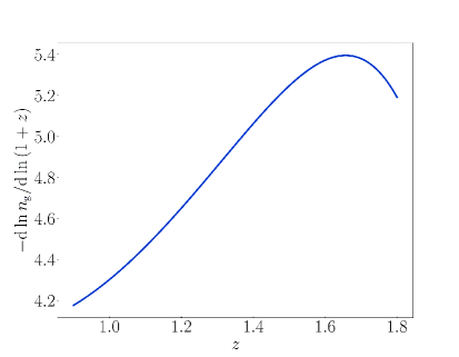
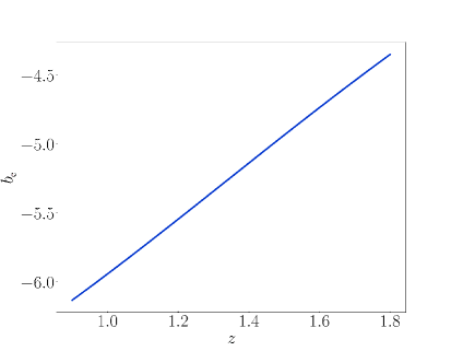
Equations (2.22)–(2.24) verify the general result (2.20), illustrating the difference between the total and partial derivatives. An example for a more realistic Stage IV H cosmological survey like Euclid or Roman is shown in Figure 1 (see subsection 2.3 for details of this model).
When dealing with survey data or simulated data, the luminosity function is in principle known as a function of luminosity in each redshift bin. Then the tracer properties can be extracted as follows.
-
•
The number density in each redshift bin is a simple luminosity integral (a sum over luminosity bins) of the luminosity function [see (2.6)].
-
•
Then the magnification bias is given by a simple ratio at the luminosity threshold of the luminosity function and the number density [see (2.14)].
-
•
By contrast, the direct expression for in (2.15) is a luminosity integral in each redshift bin of the redshift partial derivative of the luminosity function.
-
•
For , it is simpler to take a total redshift derivative of the computed number density and then algebraically compute the evolution bias via (2.20):
(2.25)
An alternative form of (2.25) is to use the observed number density contrast , which leads to
| (2.26) |
Comparing with [2], we agree with their equation (33), except for a typo: their should be replaced by the total derivative . (Without this replacement, our (2.12) shows that their equation (33) leads to .)
2.2 Simple luminosity function models
A good example of fitting a luminosity function model to data and then extracting estimates of and is given in [15] for the eBOSS quasar sample. Here we use analytical models of the luminosity function to illustrate the general features. These models are typically written in the simple form:
| (2.27) |
Here is a characteristic number density and is a characteristic luminosity. In this case, (2.6) and (2.14) lead to:
| (2.28) | |||||
| (2.29) |
For , we need
| (2.30) |
| (2.31) |
Note how the derivative of the luminosity threshold in (2.30) has been cancelled out and replaced by a derivative of in (2.31).
2.3 H survey (Euclid-/Roman-like)
As an example, we consider a Stage IV H spectroscopic survey similar to Euclid and Roman. Euclid will measure the redshifts of up to 30 million H galaxies over 15 000 in the redshift range [31]. Another H survey at higher sensitivity with the future Roman Space Telescope will cover and detect million galaxies and their redshifts over the range [29]. We first use the pre-2019 luminosity function model and then the 2019 model, in order to show how sensitive and are to the luminosity function.
Pre-2019 luminosity function model
This is the Model 1 luminosity function in [32], used at a time when the Euclid redshift range was planned as (see e.g. [33]). It is a luminosity function of Schechter type, with
| (2.34) |
in (2.27). Here is the faint-end slope and is the luminosity at which falls to 1/e of the faint-end power law. The expressions for and from [32, 33, 25] are given in subsection A.2. Figure 2 illustrates how the luminosity function varies with and .
The number density follows from (2.28):
| (2.35) |
where is the upper incomplete Gamma function. Using (2.35) in (2.29), the magnification bias is
| (2.36) |
and the evolution bias (2.31) is
| (2.37) |
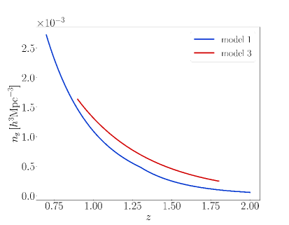
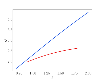
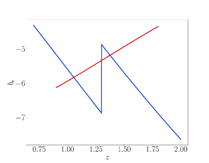
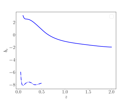
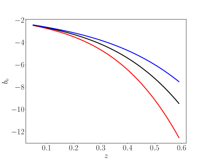
Equation (2.36) recovers the expression in [25], while (2.37) corrects an error in the published version444See arXiv:1911.02398v4 for the corrected version.. We find the blue curves shown in Figure 3 for and , using . The discontinuity in in Figure 3 (blue) arises from the Model 1 number density (A.2), which has a break at redshift . This is not a physical discontinuity, but an artefact of the modelling. The red curves in Figure 3 show an improved Model 3, which has no discontinuity (see below).
2019 luminosity function model
The updated luminosity function given by [31] is the Model 3 in [32], with a reduced redshift range . Model 3 is fit directly to the luminosity function data points and not to the analytic Schechter function, as in the case of Model 1 [32]. The luminosity function is also of the form (2.27), with the best-fit version being the broken power law case:
| (2.38) |
Here is the bright-end slope. The factor is chosen so that is the luminosity at which falls to 1/e of the faint-end power law, as in the Schechter case (2.34). The number density, magnification bias and evolution bias are given by (2.28), (2.29) and (2.31) respectively, where needs to be evaluated numerically. The expressions for and from [32] are given in subsection A.3. Using these expressions together with [31], we find the red curves shown in Figure 3 for and .
Figure 2 and Figure 3 show that the form of the luminosity function and the value of the flux cut have a significant impact on the magnification and evolution biases. In particular, even the sign of changes from Model 1 to 3. Model 3 is preferred, since it avoids the artificial discontinuity in Model 1. The physical properties of the Euclid sample determine the true luminosity function – this can be estimated via simulations and will be measured when the survey is operating.
3 Galaxy surveys with K-correction
If a survey measures galaxy fluxes in fixed wavelength bands, this leads to a K-correction for the redshifting effect on the bands. In that case, it is standard to work in terms of dimensionless magnitudes. The correction to the threshold absolute magnitude is then
| (3.1) |
where the apparent magnitude cut is . Then
| (3.2) | |||||
| (3.3) | |||||
| (3.4) |
As before, we can avoid the need to compute the integral in (3.4) as follows. We compute the total derivative:
| (3.5) |
where we used (3.3). Then this leads to a modification of (2.25) for the photometric case, using (3.1):
| (3.6) |
3.1 Bright galaxy survey (DESI-like)
For the DESI Bright Galaxy Sample (BGS), we follow [34, 16, 13], making small adjustments. DESI will conduct a ground-based optical survey covering 15 000 and expecting to detect 1.2 million bright galaxies up to [34]. We use a Schechter luminosity function of the form (2.27), with
| (3.7) |
The detailed forms for and are given in subsection A.3. The K-correction is modelled as , following [13], and we take , following [35]. The results are shown in Figure 4.
Comparing Figure 4 with Figure 3 (red), we see that the has a similar trend with redshift, but has an opposite sign. This could be due to the types of galaxies and/or to a different evolution at low and high redshifts. The true luminosity functions will be estimated when the surveys take data, and the data will determine how accurate the simple models of luminosity function are.
4 21cm Hi surveys
After the end of reionisation, nearly all Hi is contained in galaxies [36]. The 21cm emission of Hi therefore provides a tracer of the dark matter distribution. There are two types of Hi cosmological survey:
-
•
Detecting individual galaxies via the 21cm emission line, much in the same way as H and other emission-line galaxies, using the interferometer mode of the telescope.
-
•
Measuring the integrated 21cm intensity of the sky at a given frequency, without resolving individual galaxies, using either interferometer or single-dish mode.
4.1 Hi galaxy surveys (SKAO-like)
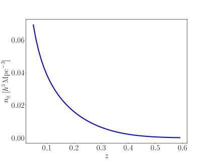
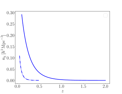
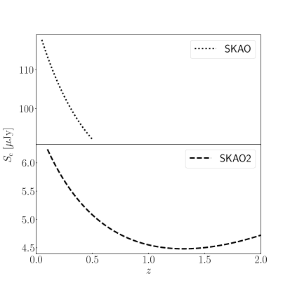
The SKAO plans to conduct a 10 000 hr Hi galaxy survey over the range and covering 5 000 deg2, detecting million galaxies [37]. This survey will use the next-generation 197-dish mid-frequency array, which will absorb the existing 64-dish MeerKAT array. A futuristic ‘Phase 2’ survey, which we denote ‘SKAO2’, could cover 30 000 deg2 over the range and detect 1 billion galaxies [38].
As in the case of optical/NIR surveys, the number density of Hi galaxies is dependent on the sensitivity threshold of the instrument. Radio surveys use the flux density , usually abbreviated as . This is the flux per frequency, in units of .
The rms noise associated with a flux density measurement by an interferometer can be approximated by [39, 38]
| (4.1) |
where is the observed frequency, with the rest-frame frequency, is the Boltzmann constant, is the system temperature (instrument + sky), is the number of dishes and is the frequency channel width. The time per pointing,
| (4.2) |
depends on the total integration time , the total survey area and the effective primary beam (field of view) from a mosaicked sky [40]:
| (4.3) |
where is the dish diameter and is the rest-frame wavelength. The effective area is
| (4.4) |
where is the aperture efficiency.
The detection limit of Hi galaxies depends not only on flux threshold, but also on the observed line profile. In order to take this into account, we include an detection threshold so that the detection is done with sufficient spectral resolution. This leads to a detection limit [39, 38]
| (4.5) |
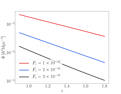
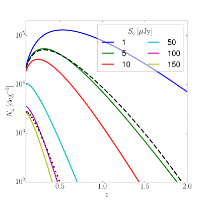
Models of an Hi luminosity function would require a relation between the Hi luminosity of a galaxy and its host dark matter halo, which depends on other factors in addition to the halo mass. This would need to be calibrated against full simulations. An alternative approach, bypassing the need for a luminosity function, is followed by [39], which uses the S3-SAX simulation. Each galaxy in the simulation has a redshift, an Hi luminosity and a line profile. This is used to determine the number of galaxies that are expected to be detected in a survey. The result is a fitting formula for the observed angular number density [39], given in terms of . We adopt this fitting formula, adjusting it to the detection threshold:
| (4.6) |
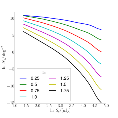
The parameters for a range of flux sensitivities are given in Table 3 of [39], together with plots of (see also [41, 38]). We provide similar plots for , against for various and against for various , in subsection A.4.
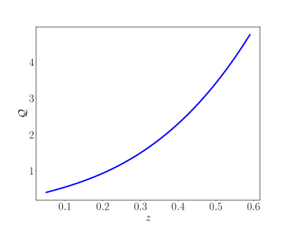
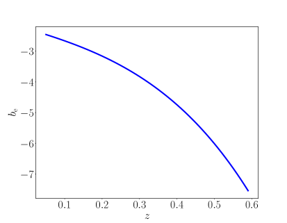
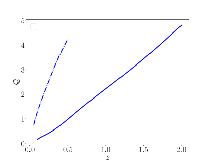
The survey specifications that we use are given in subsection A.4. The resulting comoving number density, magnification bias and evolution bias are shown in Figure 5. The magnification bias is computed from (4.6) as
| (4.7) |
which follows from (2.11), using the fact that for a fixed frequency channel width. At each fixed redshift , we define the flux densities , where and is a small increment. We compute from (4.6) for each (using suitable interpolation of Table 3 in [39]). Then we use the 5-point stencil method to compute the derivative (4.7). We tested the stability of the derivative and concluded that was a stable interval to use in this context.
This approach is related to that of [41] for an SKAO2 Hi galaxy survey, which parametrises as a function of for different redshifts (see also [9, 42, 43]).
For the evolution bias, we take the total redshift derivative of , and then use (2.25):
| (4.8) |
where has already been computed as described above.
Further details are given in subsection A.4.
4.2 Hi intensity mapping surveys (SKAO-like)
In contrast to Hi galaxy surveys, intensity mapping does not aim to detect individual Hi galaxies, but measures the total 21cm emission in each voxel (a three-dimensional pixel formed by the telescope beam and frequency channel width).
The Hi brightness temperature measured at redshift in direction is related to the observed number of 21cm emitters per redshift per solid angle, , as follows [44, 2]:
| (4.9) |
where is the angular diameter distance. This relation implies conservation of surface brightness, so that the effective magnification bias is [44, 2, 45, 26]
| (4.10) |
The evolution bias is found as follows. In the background, (4.9) implies that
| (4.11) |
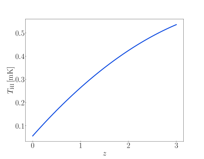
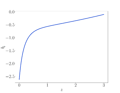
where is the comoving number density of Hi emitters in the source rest-frame. Intensity mapping integrates over the entire luminosity function in each voxel [46]. Therefore the brightness temperature does not depend on a luminosity threshold, but depends only on redshift. By (4.11), this is also the case for the number density, so that [44, 26]
| (4.12) |
Equation (4.11) also leads to [36]
| (4.13) |
where is the comoving Hi density in units of the critical density today. This is poorly constrained by current observations and we use the fit [47]:
| (4.14) |
Using (4.14), we can find the evolution bias (4.12). Figure 6 shows the temperature and evolution bias.
Note that and are survey-dependent for galaxy surveys, since they depend on the survey flux cut. By contrast, for 21cm intensity mapping there is no flux limit and the evolution bias therefore depends only on the background brightness temperature and the Hubble rate, while the effective magnification bias is 1. The evolution bias for intensity mapping has the same physical meaning as for galaxy surveys, since it given in (4.12) by the comoving number density of 21cm emitters.
5 Conclusions
The observed (linear) number density contrast depends on three astrophysical biases, which in turn depend on the sample of galaxies considered. The clustering bias has been the subject of extensive studies, but much less attention has been given to determining the magnification and evolution biases. These two biases modulate the amplitude of light-cone effects which, for forthcoming surveys, need to be included in the modeling of the two- and three-point statistics.
Forecasts for future galaxy surveys require physically self-consistent models of and , especially when lensing and other relativistic effects are important. Key examples when this is the case are:
- •
- •
- •
Our paper provides a systematic method for including and in such forecasts, which has been applied in the recent works [25, 26, 51, 43, 50, 55], that involve some of the current authors. When lensing and other relativistic effects are detectable, they can themselves provide novel probes of gravity and matter. However, such probes are only possible if magnification and evolution biases are accurately modelled [2, 48, 56, 13, 55].
The main goal of our paper was to clarify the meaning of the magnification and evolution biases and compute them for different upcoming galaxy surveys. In particular, the log total derivative of number density is not the correct expression for evolution bias; instead, this derivative must be corrected by a term involving the magnification bias, as in (2.25). The evolution bias can be positive (more galaxies in a comoving volume than the conserved case) or negative (less galaxies) and it can change sign. The magnification bias is always positive; it is most easily computed not via a derivative, but from the ratio of the luminosity function and number density, as in (2.14). Details of the computation of magnification and evolution biases differ according to the type of large-scale structure survey. We considered four types of dark matter tracers:
- optical/NIR spectroscopic galaxy surveys
-
where we used an H galaxy survey like Euclid or Roman as an example;
- optical photometric galaxy surveys
-
where we used a DESI-like bright galaxy sample as an example;
- radio spectroscopic galaxy surveys
-
where we used SKAO-like Hi galaxy surveys as examples;
- 21cm intensity maps
-
where we used an SKAO-like Hi intensity mapping survey as an example.
While spectroscopic surveys are flux-limited, photometric galaxy surveys are magnitude-limited and require an extra K-correction. Furthermore, even for the same type of spectroscopic galaxy survey, say H galaxies, the magnification and evolution biases are highly sensitive to the shape of the luminosity function. In particular, we show that depending on the model taken for the luminosity function, even the redshift slope of the evolution bias can change sign. This highlights the need to consider magnification and evolution biases when fitting luminosity functions from data, and not just the luminosity function itself. Not only will these parameters be important for future surveys, but they will also provide more information on the shape of the luminosity function. In fact, this implies that relativistic effects can be used to constrain aspects of the luminosity function.
Some simple choices of luminosity function allow us to compute and analytically, as is done in subsection 2.2. But in other cases, this is not possible – or it is numerically easier to use the total derivative of the observed number sources with the magnification bias, as shown in (2.25) and (2.30). This is the case for Hi galaxy surveys, for example. In order to perform these calculations accurately, we needed to identify and explain the subtle distinction between partial and total derivatives in the evolution bias.
An exception is provided by intensity mapping, which conserves surface brightness, so that the effective magnification bias is , independent of the survey. Similarly, the intensity mapping evolution bias is determined by the background Hi brightness temperature, independent of the survey details.
In addition to clarifications on how magnification and evolution biases are computed, we also provide fitting functions (or tables) in the Appendix for their values in the different cosmological surveys considered.
For simulated or observed galaxy data, the luminosity function is in principle known as a function of luminosity in each redshift bin. Then and may be extracted as follows.
-
•
Number density in each redshift bin is found from a simple luminosity integral (numerical sum over luminosity bins) of the luminosity function, (2.6).
-
•
Then is determined by a ratio at the luminosity threshold of the luminosity function and the number density, (2.14).
-
•
For , instead of using its definition, it is simpler to take a total redshift derivative of the computed and then use to compute via (2.25).
Acknowledgments
We thank Phil Bull for helpful discussions on detecting Hi galaxies. RM, SJ and JV acknowledge support from the South African Radio Astronomy Observatory and the National Research Foundation (Grant No. 75415). RM also acknowledges support from the UK Science & Technology Facilities Council (Grant No. ST/N000550/1). JF and CC acknowledge support from the UK STFC Consolidated Grant No. ST/P000592/1. SC acknowledges support from the ‘Departments of Excellence 2018-2022’ Grant (L. 232/2016) awarded by the Italian Ministry of University and Research (mur) and from the ‘Ministero degli Affari Esteri della Cooperazione Internazionale (maeci) – Direzione Generale per la Promozione del Sistema Paese Progetto di Grande Rilevanza ZA18GR02. This work made use of the South African Centre for High-Performance Computing, under the project Cosmology with Radio Telescopes, ASTRO-0945.
Appendix A Numerical details
A.1 Evolution bias in terms of flux
The expression (2.20) for the total derivative of number density involves the redshift-dependent luminosity cut. If we re-express in terms of and the flux cut, we need to take a little care with the total derivative:
| (A.1) |
where the vertical bars make explicit what is held constant. This equation leads to the same result as (2.20).
A.2 Euclid-/Roman-like H survey
Fitting functions for the number density, magnitude bias and evolution bias, with , are given by:
| (A.6) | |||||
| (A.7) | |||||
| (A.8) |
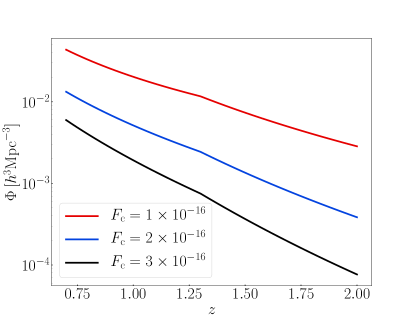
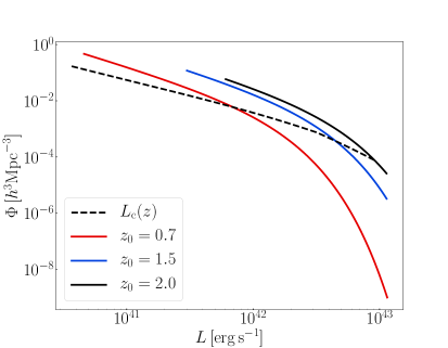
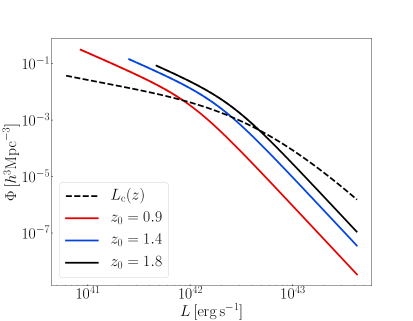
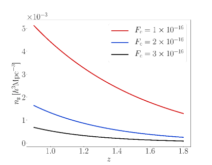
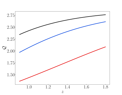
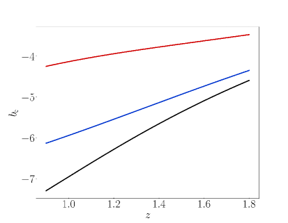
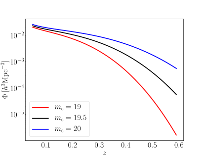
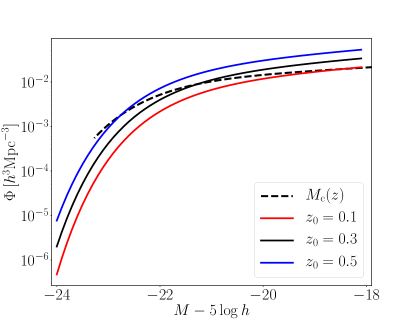
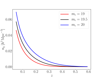
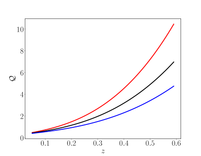
In Figure 7, we show the luminosity function at the luminosity cut against redshift for 3 different flux cuts (left), and against luminosity, at 3 redshifts (right), showing also the threshold luminosity. Figure 8 shows the associated number density, magnitude bias and evolution bias, for 3 different flux cuts.
A.3 DESI-like bright galaxy survey
The number density of the DESI BGS will closely follow the Galaxy and Mass Assembly (GAMA) survey [34, 35]. Therefore we can use the -band parameters in Table 5 of [57], with fiducial redshift (which is where the magnitudes are -corrected) in the luminosity function (3.7):
| (A.9) |
For the BGS sensitivity, we assumed , in order to include the faint sample [58]. The parameters have been slightly adjusted from [57] (within 1 uncertainty) to better represent the number densities given in Table 2 of [16].
Fitting functions for the number density, magnitude bias and evolution bias, with , are given by:
| (A.10) | |||||
| (A.11) | |||||
| (A.12) |
In Figure 9, we show the luminosity function at the absolute magnitude cut against redshift for 3 different apparent magnitude cuts (left), and against absolute magnitude, at 3 redshifts (right), showing also the threshold absolute magnitude (dashed). In Figure 10 we show the the associated number density, magnitude bias and evolution bias, for 3 different magnitude cuts.
A.4 SKAO-like Hi galaxy surveys
For both SKAO and SKAO2 surveys, we assume kHz and . For SKAO we follow the SKA Cosmology Science Working Group Red Book [37]:
| (A.13) |
where is given in [37] and the choice follows [39]. For the futuristic SKAO2, we follow [38]. We model the system temperature as
| (A.14) |
and use the survey details:
| (A.15) |
The choice follows [39]. The results for are shown in Figure 11. We also present the values of , number density, magnification bias and evolution bias, as functions of redshift, in Table 1 (SKAO) and Table 2 (SKAO2).
Fitting functions for the number density, magnitude bias and evolution bias for SKAO are:
| (A.16) | |||||
| (A.17) | |||||
| (A.18) | |||||
while for SKAO2:
| (A.19) | |||||
| (A.20) | |||||
| (A.21) | |||||
| [Jy] | [] | |||
|---|---|---|---|---|
| 0.05 | 117.58 | 1.09e-01 | 0.76 | -5.95 |
| 0.1 | 113.33 | 3.70e-02 | 1.3 | -8.15 |
| 0.15 | 109.53 | 1.48e-02 | 1.74 | -7.85 |
| 0.2 | 106.14 | 6.42e-03 | 2.14 | -7.62 |
| 0.25 | 103.11 | 2.91e-03 | 2.53 | -7.63 |
| 0.3 | 100.39 | 1.36e-03 | 2.92 | -7.84 |
| 0.35 | 97.96 | 6.56e-04 | 3.29 | -8.03 |
| 0.4 | 95.79 | 3.22e-04 | 3.63 | -7.99 |
| 0.45 | 93.85 | 1.60e-04 | 3.94 | -7.88 |
| 0.5 | 92.11 | 8.06e-05 | 4.24 | -7.76 |
| [Jy] | [] | |||
|---|---|---|---|---|
| 0.1 | 6.24 | 2.92e-01 | 0.16 | 3.09 |
| 0.2 | 5.85 | 1.62e-01 | 0.34 | 2.49 |
| 0.3 | 5.54 | 9.40e-02 | 0.51 | 2.15 |
| 0.4 | 5.28 | 5.59e-02 | 0.73 | 1.54 |
| 0.5 | 5.08 | 3.40e-02 | 0.98 | 0.85 |
| 0.6 | 4.92 | 2.10e-02 | 1.24 | 0.22 |
| 0.7 | 4.79 | 1.31e-02 | 1.49 | -0.26 |
| 0.8 | 4.68 | 8.18e-03 | 1.74 | -0.61 |
| 0.9 | 4.61 | 5.13e-03 | 1.98 | -0.87 |
| 1.0 | 4.55 | 3.21e-03 | 2.22 | -1.06 |
| 1.1 | 4.51 | 2.00e-03 | 2.45 | -1.22 |
| 1.2 | 4.49 | 1.24e-03 | 2.69 | -1.34 |
| 1.3 | 4.48 | 7.62e-04 | 2.93 | -1.45 |
| 1.4 | 4.49 | 4.63e-04 | 3.18 | -1.55 |
| 1.5 | 4.5 | 2.79e-04 | 3.44 | -1.64 |
| 1.6 | 4.53 | 1.66e-04 | 3.7 | -1.73 |
| 1.7 | 4.56 | 9.71e-05 | 3.97 | -1.81 |
| 1.8 | 4.61 | 5.61e-05 | 4.24 | -1.89 |
| 1.9 | 4.66 | 3.20e-05 | 4.52 | -1.95 |
| 2.0 | 4.72 | 1.80e-05 | 4.8 | -1.98 |
References
- [1] A. Challinor and A. Lewis, The linear power spectrum of observed source number counts, Phys. Rev. D84 (2011) 043516, [arXiv:1105.5292].
- [2] D. Alonso, P. Bull, P. G. Ferreira, R. Maartens, and M. Santos, Ultra large-scale cosmology in next-generation experiments with single tracers, Astrophys. J. 814 (2015), no. 2 145, [arXiv:1505.07596].
- [3] C. Bonvin, Effect of Peculiar Motion in Weak Lensing, Phys. Rev. D78 (2008) 123530, [arXiv:0810.0180].
- [4] D. J. Bacon, S. Andrianomena, C. Clarkson, K. Bolejko, and R. Maartens, Cosmology with Doppler Lensing, Mon. Not. Roy. Astron. Soc. 443 (2014), no. 3 1900–1915, [arXiv:1401.3694].
- [5] C. Bonvin, S. Andrianomena, D. Bacon, C. Clarkson, R. Maartens, T. Moloi, and P. Bull, Dipolar modulation in the size of galaxies: The effect of Doppler magnification, Mon. Not. Roy. Astron. Soc. 472 (2017), no. 4 3936–3951, [arXiv:1610.05946].
- [6] A. Raccanelli, D. Bertacca, D. Jeong, M. C. Neyrinck, and A. S. Szalay, Doppler term in the galaxy two-point correlation function: wide-angle, velocity, Doppler lensing and cosmic acceleration effects, Phys. Dark Univ. 19 (2018) 109–123, [arXiv:1602.03186].
- [7] F. Montanari and R. Durrer, Measuring the lensing potential with tomographic galaxy number counts, JCAP 1510 (2015), no. 10 070, [arXiv:1506.01369].
- [8] W. Cardona, R. Durrer, M. Kunz, and F. Montanari, Lensing convergence and the neutrino mass scale in galaxy redshift surveys, Phys. Rev. D94 (2016), no. 4 043007, [arXiv:1603.06481].
- [9] E. Villa, E. Di Dio, and F. Lepori, Lensing convergence in galaxy clustering in CDM and beyond, JCAP 1804 (2018), no. 04 033, [arXiv:1711.07466].
- [10] M. Ballardini and R. Maartens, Measuring ISW with next-generation radio surveys, Mon. Not. Roy. Astron. Soc. 485 (2019) 1339, [arXiv:1812.01636].
- [11] M. Jalilvand, E. Majerotto, C. Bonvin, F. Lacasa, M. Kunz, W. Naidoo, and K. Moodley, New Estimator for Gravitational Lensing Using Galaxy and Intensity Mapping Surveys, Phys. Rev. Lett. 124 (2020), no. 3 031101, [arXiv:1907.00071].
- [12] A. Witzemann, A. Pourtsidou, and M. G. Santos, Prospects for cosmic magnification measurements using H i intensity mapping, Mon. Not. Roy. Astron. Soc. 496 (2020), no. 2 1959–1966, [arXiv:1907.00755].
- [13] G. Jelic-Cizmek, F. Lepori, C. Bonvin, and R. Durrer, On the importance of lensing for galaxy clustering in photometric and spectroscopic surveys, JCAP 04 (2021) 055, [arXiv:2004.12981].
- [14] E. Di Dio and U. Seljak, The relativistic dipole and gravitational redshift on LSS, JCAP 1904 (2019), no. 04 050, [arXiv:1811.03054].
- [15] M. S. Wang, F. Beutler, and D. Bacon, Impact of Relativistic Effects on the Primordial Non-Gaussianity Signature in the Large-Scale Clustering of Quasars, Mon. Not. Roy. Astron. Soc. 499 (2020), no. 2 2598–2607, [arXiv:2007.01802].
- [16] F. Beutler and E. Di Dio, Modeling relativistic contributions to the halo power spectrum dipole, JCAP 07 (2020), no. 07 048, [arXiv:2004.08014].
- [17] P. McDonald, Gravitational redshift and other redshift-space distortions of the imaginary part of the power spectrum, JCAP 0911 (2009) 026, [arXiv:0907.5220].
- [18] C. Bonvin, L. Hui, and E. Gaztanaga, Optimising the measurement of relativistic distortions in large-scale structure, JCAP 1608 (2016), no. 08 021, [arXiv:1512.03566].
- [19] A. Hall and C. Bonvin, Measuring cosmic velocities with 21 cm intensity mapping and galaxy redshift survey cross-correlation dipoles, Phys. Rev. D95 (2017), no. 4 043530, [arXiv:1609.09252].
- [20] L. R. Abramo and D. Bertacca, Disentangling the effects of Doppler velocity and primordial non-Gaussianity in galaxy power spectra, Phys. Rev. D96 (2017), no. 12 123535, [arXiv:1706.01834].
- [21] F. Lepori, E. Di Dio, E. Villa, and M. Viel, Optimal galaxy survey for detecting the dipole in the cross-correlation with 21 cm Intensity Mapping, JCAP 1805 (2018), no. 05 043, [arXiv:1709.03523].
- [22] C. Bonvin and P. Fleury, Testing the equivalence principle on cosmological scales, JCAP 1805 (2018), no. 05 061, [arXiv:1803.02771].
- [23] F. O. Franco, C. Bonvin, and C. Clarkson, A null test to probe the scale-dependence of the growth of structure as a test of General Relativity, Mon. Not. Roy. Astron. Soc. 492 (2020), no. 1 L34–L39, [arXiv:1906.02217].
- [24] C. Clarkson, E. M. De Weerd, S. Jolicoeur, R. Maartens, and O. Umeh, The dipole of the galaxy bispectrum, Mon. Not. Roy. Astron. Soc. 486 (2019), no. 1 L101–L104, [arXiv:1812.09512].
- [25] R. Maartens, S. Jolicoeur, O. Umeh, E. M. De Weerd, C. Clarkson, and S. Camera, Detecting the relativistic galaxy bispectrum, JCAP 03 (2020) 065, [arXiv:1911.02398].
- [26] S. Jolicoeur, R. Maartens, E. M. De Weerd, O. Umeh, C. Clarkson, and S. Camera, Detecting the relativistic bispectrum in 21cm intensity maps, JCAP 06 (2021) 039, [arXiv:2009.06197].
- [27] O. Umeh, K. Koyama, and R. Crittenden, Testing the equivalence principle on cosmological scales using the odd multipoles of galaxy cross-power spectrum and bispectrum, JCAP 08 (2021) 049, [arXiv:2011.05876].
- [28] EUCLID Collaboration, R. Laureijs et al., Euclid Definition Study Report, arXiv:1110.3193.
- [29] D. Spergel et al., Wide-Field InfrarRed Survey Telescope-Astrophysics Focused Telescope Assets WFIRST-AFTA 2015 Report, arXiv:1503.03757 (2015) [arXiv:1503.03757].
- [30] D. Bertacca, Observed galaxy number counts on the light cone up to second order: III. Magnification bias, Class. Quant. Grav. 32 (2015), no. 19 195011, [arXiv:1409.2024].
- [31] Euclid Collaboration, A. Blanchard et al., Euclid preparation: VII. Forecast validation for Euclid cosmological probes, Astron. Astrophys. 642 (2020) A191, [arXiv:1910.09273].
- [32] L. Pozzetti, C. M. Hirata, J. E. Geach, A. Cimatti, C. Baugh, O. Cucciati, A. Merson, P. Norberg, and D. Shi, Modelling the number density of H emitters for future spectroscopic near-IR space missions, Astron. Astrophys. 590 (2016) A3, [arXiv:1603.01453].
- [33] V. Yankelevich and C. Porciani, Cosmological information in the redshift-space bispectrum, Mon. Not. Roy. Astron. Soc. 483 (2019), no. 2 2078–2099, [arXiv:1807.07076].
- [34] DESI Collaboration, A. Aghamousa et al., The DESI Experiment Part I: Science,Targeting, and Survey Design, arXiv:1611.00036.
- [35] O. Ruiz-Macias, P. Zarrouk, S. Cole, C. M. Baugh, P. Norberg, J. Lucey, A. Dey, D. J. Eisenstein, P. Doel, E. Gaztañaga, C. Hahn, R. Kehoe, E. Kitanidis, M. Landriau, D. Lang, J. Moustakas, A. D. Myers, F. Prada, M. Schubnell, D. H. Weinberg, and M. J. Wilson, Characterizing the target selection pipeline for the Dark Energy Spectroscopic Instrument Bright Galaxy Survey, Mon. Not. Roy. Astron. Soc. 502 (Apr., 2021) 4328–4349, [arXiv:2007.14950].
- [36] F. Villaescusa-Navarro et al., Ingredients for 21 cm Intensity Mapping, Astrophys. J. 866 (2018), no. 2 135, [arXiv:1804.09180].
- [37] SKA Collaboration, D. J. Bacon et al., Cosmology with Phase 1 of the Square Kilometre Array: Red Book 2018: Technical specifications and performance forecasts, Publ. Astron. Soc. Austral. 37 (2020) e007, [arXiv:1811.02743].
- [38] P. Bull, Extending cosmological tests of General Relativity with the Square Kilometre Array, Astrophys. J. 817 (2016), no. 1 26, [arXiv:1509.07562].
- [39] S. Yahya, P. Bull, M. G. Santos, M. Silva, R. Maartens, P. Okouma, and B. Bassett, Cosmological performance of SKA HI galaxy surveys, Mon. Not. Roy. Astron. Soc. 450 (2015), no. 3 2251–2260, [arXiv:1412.4700].
- [40] M. G. Santos, D. Alonso, P. Bull, M. Silva, and S. Yahya, HI galaxy simulations for the SKA: number counts and bias, arXiv:1501.03990.
- [41] S. Camera, M. G. Santos, and R. Maartens, Probing primordial non-Gaussianity with SKA galaxy redshift surveys: a fully relativistic analysis, Mon. Not. Roy. Astron. Soc. 448 (2015), no. 2 1035–1043, [arXiv:1409.8286].
- [42] T. Sprenger, M. Archidiacono, T. Brinckmann, S. Clesse, and J. Lesgourgues, Cosmology in the era of Euclid and the Square Kilometre Array, JCAP 02 (2019) 047, [arXiv:1801.08331].
- [43] M. Martinelli, R. Dalal, F. Majidi, Y. Akrami, S. Camera, and E. Sellentin, Ultra-large-scale approximations and galaxy clustering: debiasing constraints on cosmological parameters, arXiv:2106.15604.
- [44] A. Hall, C. Bonvin, and A. Challinor, Testing General Relativity with 21-cm intensity mapping, Phys. Rev. D 87 (2013), no. 6 064026, [arXiv:1212.0728].
- [45] M. Jalilvand, E. Majerotto, R. Durrer, and M. Kunz, Intensity mapping of the 21 cm emission: lensing, JCAP 01 (2019) 020, [arXiv:1807.01351].
- [46] P. C. Breysse, E. D. Kovetz, P. S. Behroozi, L. Dai, and M. Kamionkowski, Insights from probability distribution functions of intensity maps, Mon. Not. Roy. Astron. Soc. 467 (2017), no. 3 2996–3010, [arXiv:1609.01728].
- [47] MeerKLASS Collaboration, M. G. Santos et al., MeerKLASS: MeerKAT Large Area Synoptic Survey, 2017. arXiv:1709.06099.
- [48] D. Alonso and P. G. Ferreira, Constraining ultralarge-scale cosmology with multiple tracers in optical and radio surveys, Phys. Rev. D 92 (2015), no. 6 063525, [arXiv:1507.03550].
- [49] J. Fonseca, S. Camera, M. Santos, and R. Maartens, Hunting down horizon-scale effects with multi-wavelength surveys, Astrophys. J. 812 (2015), no. 2 L22, [arXiv:1507.04605].
- [50] J.-A. Viljoen, J. Fonseca, and R. Maartens, Multi-wavelength spectroscopic probes: prospects for primordial non-Gaussianity and relativistic effects, JCAP 11 (2021) 010, [arXiv:2107.14057].
- [51] R. Maartens, S. Jolicoeur, O. Umeh, E. M. De Weerd, and C. Clarkson, Local primordial non-Gaussianity in the relativistic galaxy bispectrum, JCAP 04 (2021) 013, [arXiv:2011.13660].
- [52] S. Camera, R. Maartens, and M. G. Santos, Einstein’s legacy in galaxy surveys, Mon. Not. Roy. Astron. Soc. 451 (2015), no. 1 L80–L84, [arXiv:1412.4781].
- [53] S. Camera, C. Carbone, C. Fedeli, and L. Moscardini, Neglecting primordial non-Gaussianity threatens future cosmological experiment accuracy, Phys. Rev. D 91 (Feb., 2015) 043533, [arXiv:1412.5172].
- [54] A. Kehagias, A. M. Dizgah, J. Noreña, H. Perrier, and A. Riotto, A Consistency Relation for the Observed Galaxy Bispectrum and the Local non-Gaussianity from Relativistic Corrections, JCAP 1508 (2015), no. 08 018, [arXiv:1503.04467].
- [55] J.-A. Viljoen, J. Fonseca, and R. Maartens, Multi-wavelength spectroscopic probes: biases from neglecting light-cone effects, JCAP (2021) in press, [arXiv:2108.05746].
- [56] C. S. Lorenz, D. Alonso, and P. G. Ferreira, Impact of relativistic effects on cosmological parameter estimation, Phys. Rev. D 97 (2018), no. 2 023537, [arXiv:1710.02477].
- [57] J. Loveday, P. Norberg, I. K. Baldry, S. P. Driver, A. M. Hopkins, J. A. Peacock, S. P. Bamford, J. Liske, J. Bland-Hawthorn, S. Brough, M. J. I. Brown, E. Cameron, C. J. Conselice, S. M. Croom, C. S. Frenk, M. Gunawardhana, D. T. Hill, D. H. Jones, L. S. Kelvin, K. Kuijken, R. C. Nichol, H. R. Parkinson, S. Phillipps, K. A. Pimbblet, C. C. Popescu, M. Prescott, A. S. G. Robotham, R. G. Sharp, W. J. Sutherland, E. N. Taylor, D. Thomas, R. J. Tuffs, E. van Kampen, and D. Wijesinghe, Galaxy and Mass Assembly (GAMA): ugriz galaxy luminosity functions, Mon. Not. Roy. Astron. Soc. 420 (Feb., 2012) 1239–1262, [arXiv:1111.0166].
- [58] O. Ruiz-Macias, P. Zarrouk, S. Cole, P. Norberg, C. Baugh, D. Brooks, A. Dey, Y. Duan, S. Eftekharzadeh, D. J. Eisenstein, J. E. Forero-Romero, E. Gaztañaga, C. Hahn, R. Kehoe, M. Landriau, D. Lang, M. E. Levi, J. Lucey, A. M. Meisner, J. Moustakas, A. D. Myers, N. Palanque-Delabrouille, C. Poppett, F. Prada, A. Raichoor, D. J. Schlegel, M. Schubnell, G. Tarlé, D. H. Weinberg, M. J. Wilson, and C. Yèche, Preliminary Target Selection for the DESI Bright Galaxy Survey (BGS), Research Notes of the American Astronomical Society 4 (Oct., 2020) 187, [arXiv:2010.11283].